
Accurate Sum and Dot Product with New Instruction for High-Precision Computing on ARMv8 Processor

Abstract
1. Introduction
1.1. Previous Work
1.2. Background
1.2.1. Notation
1.2.2. Error-Free Transformation
| Algorithm 1 TwoSum [2] |
| Algorithm 2 TwoProductFMA [6] |
1.2.3. Compensated Summation and Dot
| Algorithm 3 CompensatedSum [6] |
|
| Algorithm 4 CompensatedDot [6] |
|
2. Compensated Sum and Dot Product Algorithms Based on High-Precision Instructions
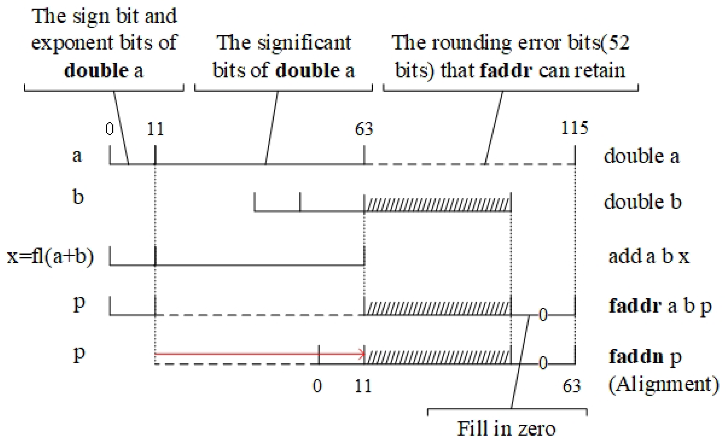
2.1. The Faddr and Faddn Instructions
| Algorithm 5 Err |
- (a)
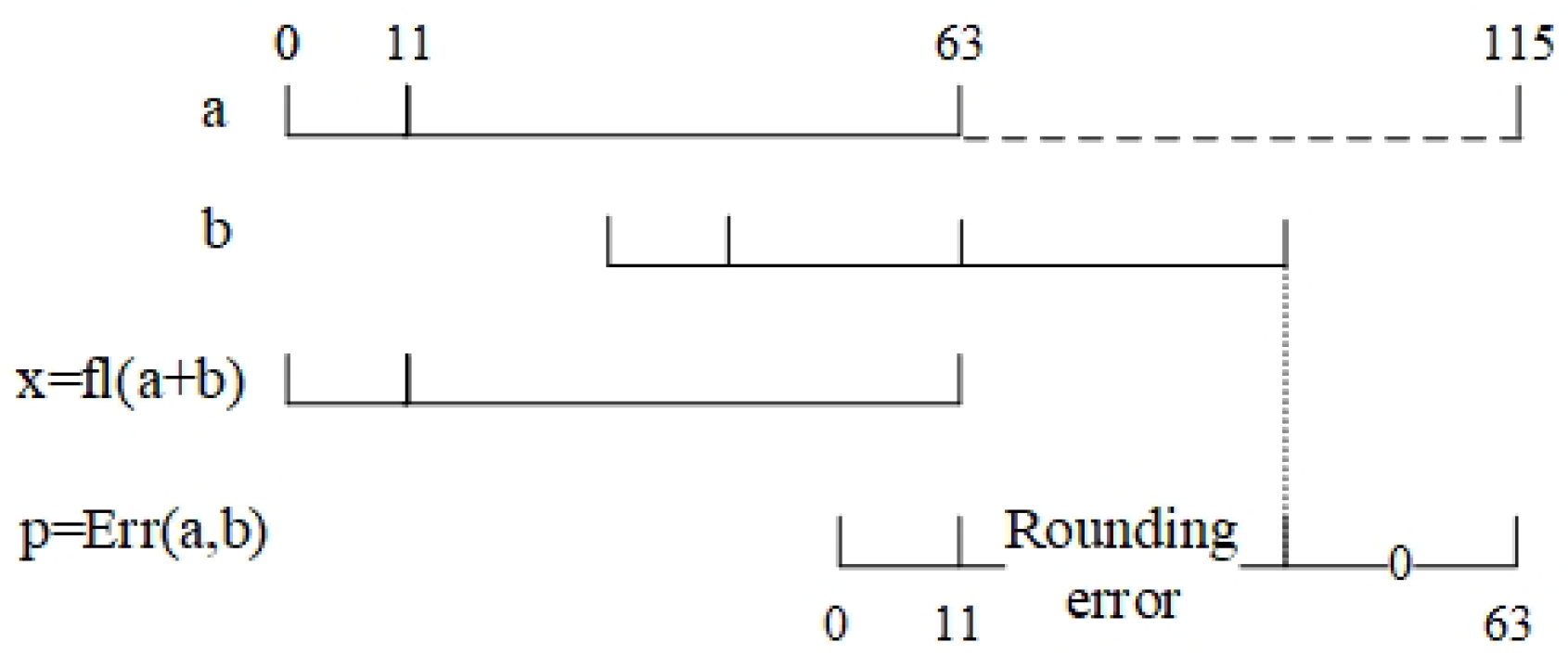
- When , there is no rounding error. p, the rounding error, and zero are equal, as shown in Figure 2.

- (b)
- (c)
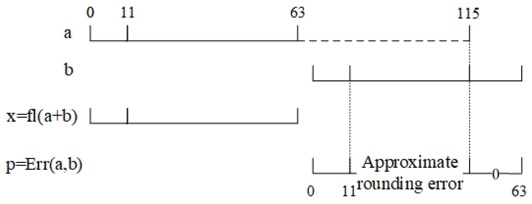
- When and , due to the limitation of the instructions, part of the rounding error will be truncated. Therefore, p is the approximation of the rounding error, as shown in Figure 4.
- (d)
- When , the rounding error is too small to be retained. Therefore, p equals zero, as shown in Figure 5.

2.2. Compensated Summation and Dot Product Based on High-Precision Instructions
| Algorithm 6 rnTwoSum |
| Algorithm 7 rnCompensatedSum |
|
| Algorithm 8 rnCompensatedDot |
|
2.3. Error Analysis
- (a)
- , ;
- (b)
- When , ; when , ;
- (c)
- When , ; when , .
3. Numerical Experiment
| Listing 1. The code to modify the rounding mode on the ARMv8 platform. |
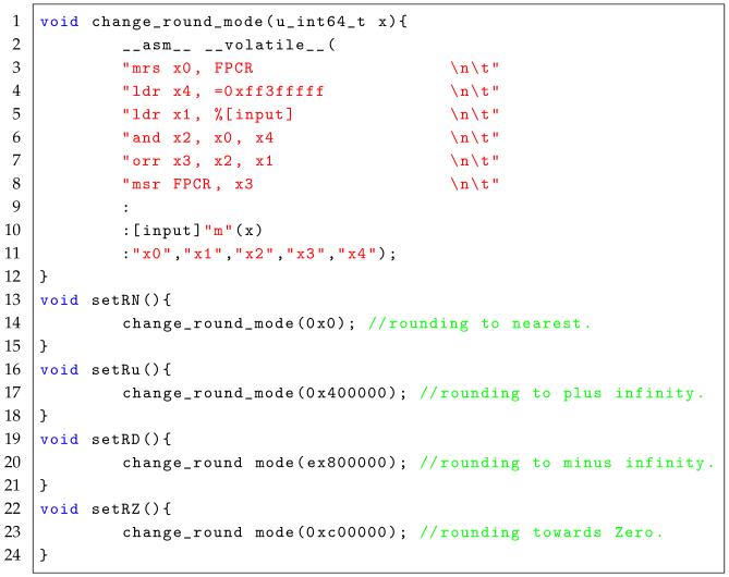 |
3.1. FPGA Hardware Simulation Platform
3.2. Experiment for Accurate Summation
3.2.1. Accuracy Comparison for Accurate Summation
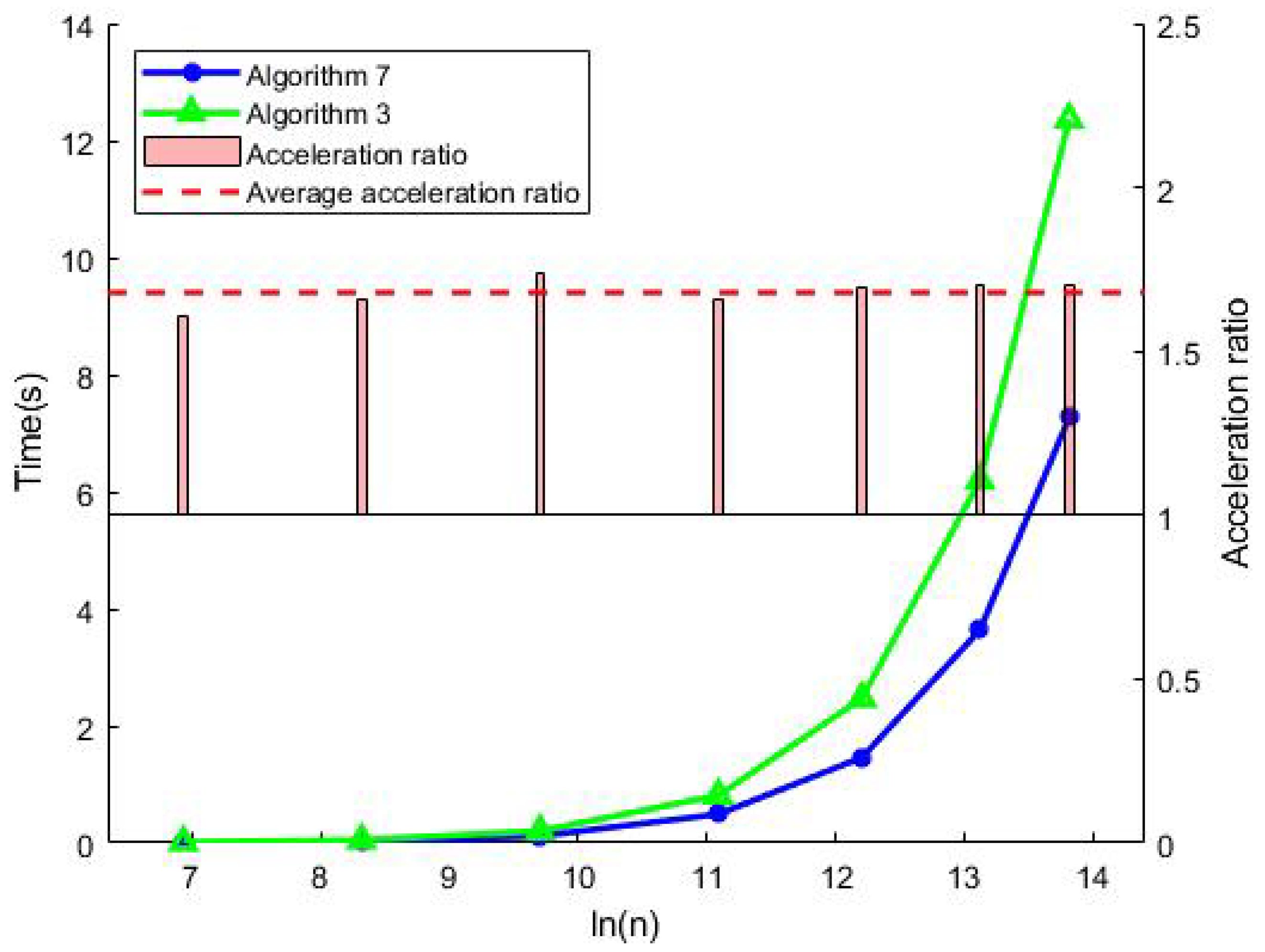
3.2.2. Runtime Performance Comparison for Accurate Summation
3.3. Experiment for Accurate Dot Product
3.3.1. Accuracy Comparison for Accurate Dot Product
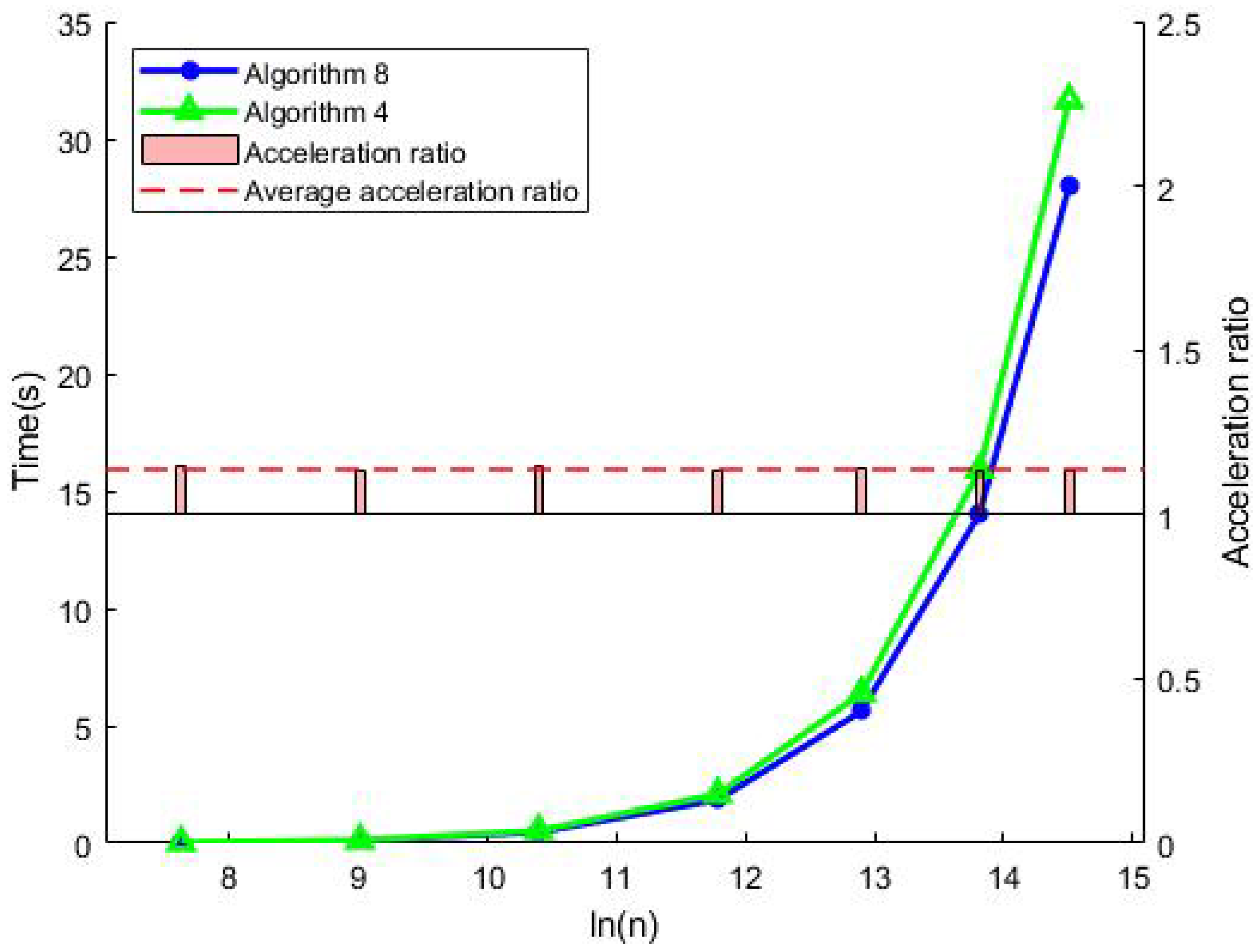
3.3.2. Runtime Performance Comparison for Accurate Dot Product
4. Conclusions
Author Contributions
Funding
Data Availability Statement
Conflicts of Interest
References
- Kahan, W. Pracniques: Further remarks on reducing truncation errors. Commun. ACM 1965, 8, 40. [Google Scholar] [CrossRef]
- Knuth, D.E. The Art of Computer Programming: Seminumerical Algorithms, 3rd ed.; Addison-Wesley Longman Publishing Co., Inc.: Reading, MA, USA, 1997; Volume 2. [Google Scholar]
- Boldo, S.; Graillat, S.; Muller, J.M. On the robustness of the 2sum and fast2sum algorithms. ACM Trans. Math. Softw. 2017, 44, 4. [Google Scholar] [CrossRef]
- Dekker, T.J. A floating-point technique for extending the available precision. Numer. Math. 1971, 18, 224–242. [Google Scholar] [CrossRef]
- Graillat, S.; Lefèvre, V.; Muller, J.M. Alternative split functions and dekker’s product. In Proceedings of the 2020 IEEE 27th Symposium on Computer Arithmetic (ARITH), Portland, OR, USA, 7–10 June 2020; pp. 41–47. [Google Scholar] [CrossRef]
- Ogita, T.; Rump, S.M.; Oishi, S. Accurate sum and dot product. SIAM J. Sci. Comput. 2005, 26, 1955–1988. [Google Scholar] [CrossRef]
- Rump, S.M.; Ogita, T.; Oishi, S. Accurate floating-point summation part I: Faithful rounding. SIAM J. Sci. Comput. 2008, 31, 189–224. [Google Scholar] [CrossRef]
- Rump, S.M.; Ogita, T.; Oishi, S. Accurate floating-point summation part II: Sign, k-fold faithful and rounding to nearest. SIAM J. Sci. Comput. 2009, 31, 1269–1302. [Google Scholar] [CrossRef]
- Yamanaka, N.; Ogita, T.; Rump, S.M.; Oishi, S. A parallel algorithm for accurate dot product. Parallel Comput. 2008, 34, 392–410. [Google Scholar] [CrossRef]
- Ozaki, K.; Ogita, T.; Oishi, S.; Rump, S.M. Error-free transformations of matrix multiplication by using fast routines of matrix multiplication and its applications. Numer. Algorithms 2012, 59, 95–118. [Google Scholar] [CrossRef]
- Graillat, S.; Ménissier-Morain, V. Accurate summation, dot product and polynomial evaluation in complex floating point arithmetic. Inf. Comput. 2012, 216, 57–71. [Google Scholar] [CrossRef]
- Kadric, E.; Gurniak, P.; Dehon, A. Accurate parallel floating-point accumulation. In Proceedings of the 2013 IEEE 21st Symposium on Computer Arithmetic, Austin, TX, USA, 7–10 April 2013; pp. 153–162. [Google Scholar] [CrossRef]
- Demmel, J.; Nguyen, H.D. Fast reproducible floating-point summation. In Proceedings of the 2013 IEEE 21st Symposium on Computer Arithmetic, ARITH ’13, Austin, TX, USA, 7–10 April 2013; pp. 163–172. [Google Scholar] [CrossRef]
- Abdalla, D.M.; Zaki, A.M.; Bahaa-Eldin, A.M. Acceleration of accurate floating point operations using SIMD. In Proceedings of the 2014 9th international conference on computer engineering & systems (ICCES), Cairo, Egypt, 22–23 December 2014; pp. 225–230. [Google Scholar] [CrossRef]
- Jankovic, J.; Subotic, M.; Marinkovic, V. One solution of the accurate summation using fixed-point accumulator. In Proceedings of the 2015 23rd Telecommunications Forum Telfor (TELFOR), Belgrade, Serbia, 24–26 November 2015; pp. 508–511. [Google Scholar] [CrossRef]
- Goodrich, M.T.; Eldawy, A. Parallel algorithms for summing floating-point numbers. In Proceedings of the 28th ACM Symposium on Parallelism in Algorithms and Architectures, SPAA ’16, New York, NY, USA, 11–13 July 2016; pp. 13–22. [Google Scholar] [CrossRef]
- Evstigneev, N.; Ryabkov, O.; Bocharov, A.; Petrovskiy, V.; Teplyakov, I. Compensated summation and dot product algorithms for floating-point vectors on parallel architectures: Error bounds, implementation and application in the Krylov subspace methods. J. Comput. Appl. Math. 2022, 414, 114434. [Google Scholar] [CrossRef]
- Lange, M. Toward accurate and fast summation. ACM Trans. Math. Softw. 2022, 48, 28. [Google Scholar] [CrossRef]
- Zhu, Y.K.; Hayes, W.B. Correct rounding and a hybrid approach to exact floating-point summation. SIAM J. Sci. Comput. 2009, 31, 2981–3001. [Google Scholar] [CrossRef]
- Jiang, H.; Du, Q.; Guo, M.; Quan, Z.; Zuo, K.; Wang, F.; Yang, C.Q. Design and implementation of qgemm on armv8 64-bit multi-core processor. Jisuanji Xuebao/Chin. J. Comput. 2017, 40, 2018–2029. [Google Scholar]
- Lange, M.; Rump, S.M. Error estimates for the summation of real numbers with application to floating-point summation. BIT Numer. Math. 2017, 57, 927–941. [Google Scholar] [CrossRef]
- Lange, M.; Rump, S. Sharp estimates for perturbation errors in summations. Math. Comput. 2018, 88, 349–368. [Google Scholar] [CrossRef]
- Boldo, S.; Lauter, C.; Muller, J.M. Emulating round-to-nearest ties-to-zero “augmented” floating-point operations using round-to-nearest ties-to-even arithmetic. IEEE Trans. Comput. 2021, 70, 1046–1058. [Google Scholar] [CrossRef]
- Muller, J.M.; Rideau, L. Formalization of double-word arithmetic, and comments on “tight and rigorous error bounds for basic building blocks of double-word arithmetic”. ACM Trans. Math. Softw. 2022, 48, 15res. [Google Scholar] [CrossRef]
- Brisebarre, N.; Muller, J.M.; Picot, J. Error in ulps of the multiplication or division by a correctly-rounded function or constant in binary floating-point arithmetic. In Proceedings of the 2023 IEEE 30th Symposium on Computer Arithmetic (ARITH), Portland, OR, USA, 4–6 September 2023; p. 88. [Google Scholar] [CrossRef]
- Hubrecht, T.; Jeannerod, C.P.; Muller, J.M. Useful applications of correctly-rounded operators of the form ab + cd + e. In Proceedings of the 2024 IEEE 31st Symposium on Computer Arithmetic (ARITH), Malaga, Spain, 10–12 June 2024; pp. 32–39. [Google Scholar] [CrossRef]
- IEEE-Std-754-2019; IEEE Standard for Floating-Point Arithmetic. Technical Report; IEEE Computer Society: New York, NY, USA, 2019. [Google Scholar] [CrossRef]
- Higham, N.J. Accuracy and Stability of Numerical Algorithms, 2nd ed.; Society for Industrial and Applied Mathematics: Philadelphia, PA, USA, 2002. [Google Scholar]

| Condition Number | Relative Error of Algorithm 7 (Ours) | Relative Error of Algorithm 3 [6] | Relative Error of Classic Sum |
|---|---|---|---|
| 6.51898903 | 0.00000000 | 0.00000000 | 2.21007546 |
| 2.60759465 | 0.00000000 | 0.00000000 | 3.63575381 |
| 1.04303784 | 0.00000000 | 0.00000000 | 5.83473446 |
| 4.17215134 | 0.00000000 | 0.00000000 | 9.34421480 |
| 1.27323954 | 0.00000000 | 0.00000000 | 7.02761044 |
| 3.18309886 | 0.00000000 | 0.00000000 | 5.47924835 |
| 6.36619772 | 0.00000000 | 0.00000000 | 2.19175222 |
| 6.51898903 | 0.00000000 | 0.00000000 | 2.20868596 |
| 2.60750465 | 0.00000000 | 0.00000000 | 3.63419377 |
| 1.04303784 | 6.46234854 | 6.46234854 | 5.83543333 |
| 4.17215134 | 8.91804098 | 8.91804098 | 9.34405709 |
| 1.27323954 | 7.50024900 | 7.50924900 | 7.02764015 |
| 3.18309886 | 7.50024900 | 7.50924900 | 5.47923314 |
| 6.36619772 | 2.19267486 | 2.19267486 | 2.19175070 |
| 2.60759465 | 2.11611938 | 9.57846791 | 3.63533640 |
| 1.04303784 | 8.57846791 | 1.11976044 | 5.83497916 |
| 4.17215134 | 3.18771198 | 3.18771198 | 9.34401167 |
| 1.27323054 | 3.62749365 | 3.62749365 | 7.02763561 |
| 3.18309886 | 3.62749365 | 1.09506612 | 5.47925087 |
| 6.36619772 | 3.21264849 | 3.21264849 | 2.19175611 |
| Condition Number | Relative Error of Algorithm 8 (Ours) | Relative Error of Algorithm 4 [6] | Relative Error of Classic Dot |
|---|---|---|---|
| 3.09609813 | 0.00000000 | 0.00000000 | 3.64059902 |
| 4.93847415 | 0.00000000 | 0.00000000 | 5.84336469 |
| 7.78222147 | 0.00000000 | 0.00000000 | 9.34442157 |
| 3.09609813 | 0.00000000 | 0.00000000 | 3.64271123 |
| 1.24410327 | 0.00000000 | 0.00000000 | 1.49551930 |
| 4.93847415 | 0.00000000 | 0.00000000 | 5.84243904 |
| 3.09609813 | 0.00000000 | 0.00000000 | 3.64190617 |
| 1.24410327 | 1.29172524 | 5.23042845 | 1.49552064 |
| 1.15696185 | 2.97732081 | 1.19008129 | 1.12452736 |
| 7.22410536 | 5.95210052 | 2.38306367 | 8.76712204 |
| 2.89045729 | 4.76318389 | 1.00464464 | 3.50684910 |
| 1.24410327 | 1.31147418 | 5.23462639 | 1.49552170 |
| 1.15696185 | 2.97807148 | 1.19010342 | 1.12453110 |
| 7.22410535 | 5.95217559 | 2.38305000 | 8.76713306 |
| 2.89045729 | 4.76325403 | 1.90464327 | 3.50685311 |
| Algorithm | FLOPs | Relative Error Bound |
|---|---|---|
| Algorithm 3 | (Theorem 2) | |
| Algorithm 7 | (Theorem 4) | |
| Algorithm 4 | (Theorem 3) | |
| Algorithm 8 | (Theorem 5) |
Disclaimer/Publisher’s Note: The statements, opinions and data contained in all publications are solely those of the individual author(s) and contributor(s) and not of MDPI and/or the editor(s). MDPI and/or the editor(s) disclaim responsibility for any injury to people or property resulting from any ideas, methods, instructions or products referred to in the content. |
© 2025 by the authors. Licensee MDPI, Basel, Switzerland. This article is an open access article distributed under the terms and conditions of the Creative Commons Attribution (CC BY) license (https://creativecommons.org/licenses/by/4.0/).
Share and Cite
Xie, K.; Lu, Q.; Jiang, H.; Wang, H. Accurate Sum and Dot Product with New Instruction for High-Precision Computing on ARMv8 Processor. Mathematics 2025, 13, 270. https://doi.org/10.3390/math13020270
Xie K, Lu Q, Jiang H, Wang H. Accurate Sum and Dot Product with New Instruction for High-Precision Computing on ARMv8 Processor. Mathematics. 2025; 13(2):270. https://doi.org/10.3390/math13020270
Chicago/Turabian StyleXie, Kaisen, Qingfeng Lu, Hao Jiang, and Hongxia Wang. 2025. "Accurate Sum and Dot Product with New Instruction for High-Precision Computing on ARMv8 Processor" Mathematics 13, no. 2: 270. https://doi.org/10.3390/math13020270
APA StyleXie, K., Lu, Q., Jiang, H., & Wang, H. (2025). Accurate Sum and Dot Product with New Instruction for High-Precision Computing on ARMv8 Processor. Mathematics, 13(2), 270. https://doi.org/10.3390/math13020270