Hybrid Algorithm via Reciprocal-Argument Transformation for Efficient Gauss Hypergeometric Evaluation in Wireless Networks

Abstract

The rapid densification of wireless networks demands efficient evaluation of special functions underpinning system-level performance metrics. To facilitate research, we introduce a computational framework tailored for the zero-balanced Gauss hypergeometric function $\Psi (x,y)\triangleq {}_{2}F_1(1,x;1+x;-y)$, a fundamental mathematical kernel emerging in Signal-to-Interference-plus-Noise Ratio (SINR) coverage analysis of non-uniform cellular deployments. Specifically, we propose a novel Reciprocal-Argument Transformation Algorithm (RTA), derived rigorously from a Mellin–Barnes reciprocal-argument identity, achieving geometric convergence with $O\left(1/y\right)$. By integrating RTA with a Pfaff-series solver into a hybrid algorithm guided by a golden-ratio switching criterion, our approach ensures optimal efficiency and numerical stability. Comprehensive validation demonstrates that the hybrid algorithm reliably attains machine-precision accuracy ($\sim {10}^{-16}$) within 1 μs per evaluation, dramatically accelerating calculations in realistic scenarios from hours to fractions of a second. Consequently, our method significantly enhances the feasibility of tractable optimization in ultra-dense non-uniform cellular networks, bridging the computational gap in large-scale wireless performance modeling.

1. Introduction

The Gauss hypergeometric function ${}_{2}F_1(a,b;c;z)$ is one of the most ubiquitous special functions in mathematics and physics. Since Gauss’s classical work established its fundamental properties [1], ${}_{2}F_1$ has been recognized as a “universal” function encompassing a wide array of elementary and special functions. In modern applications, the hypergeometric function plays a crucial role across disciplines, from quantum mechanics and quantum field theory [2,3] to finance and statistics [4]. In wireless communications theory, ${}_{2}F_1$ frequently appears in closed-form solutions for performance metrics such as signal coverage probability, connection reliability, and outage probability [5,6,7].

A particularly significant case is the degenerate form $\Psi (x,y)\triangleq {}_{2}F_1\left(1,x;1+x;-y\right)$, which naturally arises when evaluating integrals in stochastic-geometry models of cellular networks [5,7]. As highlighted by Cai et al. [5] and others [6,7], it emerges as central to formulas for coverage and link reliability in 5G and heterogeneous networks. In composite fading channels such as $\kappa$–$\mu$ and $\eta$–$\mu$ channels, closed-form solutions for symbol-error rates and outage probabilities reduce to $\Psi (x,y)$, where $x\propto 1/\mu$ and y is proportional to the instantaneous Signal-to-Noise Ratio (SNR) [6]. In secrecy and covert communication systems, integrals of the form ${\int }_0^1{t}^{x-1}/(1+yt)dt$ evaluate exactly to $x^{-1}\Psi (x,y)$, linking eavesdropper coverage directly to $\Psi$ [8]. In stochastic-geometry modeling of cellular networks, when base stations are distributed according to a non-uniform Poisson point process within a finite disk, the Laplace transform of aggregate interference involves $\Psi (k/\eta ,·)$, where k takes values such as 2, 3, and 4, in its angular integral. A notable example is the coverage-probability framework introduced by Pratt et al. [9], where position-dependent Signal-to-Interference-plus-Noise Ratio (SINR) coverage in ultra-dense regions is expressed through repeated evaluations of $\Psi$, embedded in a double integral over user location and nearest-neighbor distance. These applications highlight the pivotal role of $\Psi (x,y)$ in wireless communication, serving as an essential mathematical tool for analyzing network performance.

Despite its importance, the computational evaluation of Gauss hypergeometric functions remains challenging. The defining series converges only for $\left|z\right|<1$, so direct summation for $\Psi (x,y)$ works only when $\left|y\right|<1$ and diverges when $y\ge 1$ [5]. Even inside the unit disc, convergence may be slow if parameters are large or y is close to 1. Therefore, efficient evaluation relies on analytic continuation, transformation formulas, and asymptotics [4,10]. Classical linear transformations are invaluable. Using Pfaff’s transformation [11], Cai et al. [5] obtain ${}_{2}F_1(1,x;1+x;-y)={\displaystyle \frac{1}{1+y}}{}_{2}F_1\left(1,1;1+x;\frac{y}{1+y}\right)$, yielding a rapidly convergent series in $1/(1+y)$ for large y. However, even with Pfaff’s transformation, significant inefficiency persists when $y\gg 1$. As y increases, the transformed argument $y/(1+y)$ approaches unity, placing the Gauss hypergeometric series at the boundary of its convergence domain. Consequently, the series ${}_{2}F_1(1,1;1+x;y/(1+y))$ converges very slowly, and an increasingly large number of terms must be summed to attain a fixed precision. The practical effect is a steep increase in computational cost, and the accumulation of rounding errors from summing many terms degrades numerical stability.

These issues become particularly acute in large-scale simulations and iterative computations typical in wireless communications and other fields, where ${}_{2}F_1$ evaluations may be performed millions of times. In such settings, the slow convergence of the Pfaff-transformed series can dominate the overall runtime and propagate errors across evaluations, undermining both efficiency and accuracy. Motivated by these limitations, this paper develops a new algorithm for efficiently evaluating $\Psi (x,y)$ in the regime $y\gg 1$. The proposed method employs a novel series representation that remains rapidly convergent even as y becomes large, thereby overcoming the shortcomings of existing approaches. This work provides the theoretical framework and numerical analysis demonstrating the improved performance of the new algorithm compared to classical transformations. Specially, our contributions to this work are as follows:

(1)

We derive from the Mellin–Barnes integral and construct a fast solver that eliminates the slow-convergence bottleneck of the Pfaff series for large y.

(2)

We analytically determine the optimal switch between reciprocal and Pfaff forms, producing a hybrid algorithm that is uniformly efficient for all $y>0$ and keeps the error at roughly ${10}^{-16}$.

(3)

We prove geometric convergence and rigorously bound round-off propagation, thereby guaranteeing numerical stability across the entire parameter space.

(4)

Through extensive experiments, we demonstrate up to ${10}^4\times$ speed-ups over widely used built-in implementations and achieve at least a thousandfold reduction in runtime for ultra-dense network simulations while preserving high numerical precision.

2. Related Works

The Gauss hypergeometric function ${}_{2}F_1(a,b;c;z)$ is a classical special function with significant applications across pure and applied mathematics [12,13]. Its fundamental properties, including satisfying a second-order differential equation, are extensively documented in standard references [12,14]. Historically, Gauss leveraged ${}_{2}F_1$ extensively in elliptic integral theory, where the complete elliptic integral of the first kind is compactly represented as $K\left(k\right)={\displaystyle \frac{\pi }{2}}{}_{2}F_1(\frac{1}{2},\frac{1}{2};1;k^2)$ [12,14]. More broadly, ${}_{2}F_1$ subsumes numerous elementary and special functions such as binomial series and Legendre functions, underscoring its ubiquity in theoretical physics and engineering contexts [13,14]. Indeed, hypergeometric functions frequently appear when integrals or series require analytic continuation beyond elementary forms; solutions of Laplace’s equation in spherical and cylindrical coordinates often involve ${}_{2}F_1$ or its confluent limits [13,14]. Beyond classical scalar scenarios, recent advancements have significantly generalized hypergeometric functions. Cuchta et al. systematically developed discrete and matrix-valued hypergeometric series, elucidating intricate convergence conditions and divergence criteria essential for numerical stability and practical computations [15,16,17]. In particular, Cuchta’s work has advanced discrete hypergeometric series, highlighting their applicability to difference equations and discrete analogues of classical special functions [15,16]. Distinct from these generalized formulations, the two-variable scalar function $\Psi (x,y)$ has emerged as noteworthy in applied analysis. Originally arising in analytic number theory as the count of y-smooth integers up to x, its asymptotic behavior was first studied by Dickman [18], refined by de Bruijn [19], and further advanced by Hildebrand and Tenenbaum [20]. The function $\Psi (x,y)$ is also integral to integer factorization algorithms, particularly in analyzing the distribution of smooth numbers [18,20]. Furthermore, $\Psi (x,y)$ prominently appears in SINR coverage analysis within wireless communications, especially in non-uniform cellular network deployments, necessitating efficient numerical computation methods. Thus, while Cuchta’s seminal contributions emphasize broader generalizations and theoretical frameworks, our current work provides tailored algorithmic solutions optimized specifically for rapid, numerically stable evaluations of $\Psi (x,y)$ in practical, large-scale wireless scenarios. By clearly delineating these parallel yet complementary research streams, our study bridges classical analytic theory and modern computational demands, enhancing the feasibility of tractable optimization in real-world applications.

Special functions such as ${}_{2}F_1$ and $\Psi (x,y)$ frequently appear in closed-form performance metrics for wireless communications, underpinning critical parameters like coverage, connection probability, outage, ergodic capacity, and error rates [5,21]. For instance, the Gaussian hypergeometric function ${}_{2}F_1(1,x;1+x;-y)$ arises naturally in cellular coverage and outage probability analyses [5]. Coverage probabilities and SINR thresholds often involve integrals expressible neatly as ${}_{2}F_1$ [21,22], commonly observed in stochastic geometry approaches to wireless network analysis. Notably, Jo et al. employed hypergeometric functions in downlink evaluations of heterogeneous networks [22], while Zhang et al. utilized similar methods to establish coverage bounds for multi-slope path-loss models [21]. Recent studies in ultra-dense networks (UDNs) further underline the importance of managing interference, efficient resource allocation, and energy utilization under extremely dense conditions, thus highlighting potential avenues where special functions like $\Psi (x,y)$ could significantly contribute to analytical simplification and computational efficiency. Moghaddam and Ashoor [23] developed a Kuhn–Munkres-based resource allocation algorithm improving throughput and user connectivity, while Stoynov et al. [24] provided a comprehensive taxonomy emphasizing key performance indicators and interference mitigation. Cho et al. [25] discussed critical challenges and emerging technologies required for 6G densification scenarios, highlighting the necessity for intelligent interference control. Furthermore, Kwong et al. [26] introduced a reinforcement learning framework optimizing handover parameters, and Kim and Kim [27] proposed coordinated multi-point transmission methods to significantly reduce interference in UDNs. Thus, the role of special functions such as $\Psi (x,y)$ extends beyond mere mathematical convenience, potentially offering vital analytical tools to manage and optimize performance in increasingly complex ultra-dense network environments.

The numerical evaluation of ${}_{2}F_1$ and related functions has been the subject of extensive research. Classic references present numerous linear and quadratic transformations (Euler, Pfaff, etc.) and contiguous relations [12,14]. In particular, the Pfaff transformation and its variants are widely used to move the argument z of ${}_{2}F_1$ into regions of convergence [12,14]. By these identities, Cai et al. [5] accelerate ${}_{2}F_1(1,x;1+x;-y)$ by a Pfaff-transformed algorithm, yet the sole reliance on this form causes slow convergence and rising cost as $y\gg 1$. Earlier, Forrey developed a general “transformation theory” for ${}_{2}F_1$ (restricting to real parameters) to avoid cancellation and slow convergence [28]. Michel and Stoitsov extended such ideas to the complex-parameter case, combining series expansions with analytic continuation to compute ${}_{2}F_1$ reliably [3]. These works underline that applying Pfaff and Euler transforms is a key computational strategy. Despite these advances, existing methods often target particular parameter ranges. For arbitrary parameters, the algorithm of Michel and Stoitsov [3] or Forrey’s method [28] remain among the most general but can become unstable if parameters are large or near singularities. These gaps motivate us to study the efficient and robust evaluation of $\Psi (x,y)$.

3. Preliminaries

3.1. Gauss Hypergeometric Function and the Special Case ${}_{2}F_1(1,x;1+x;-y)$

The Gauss hypergeometric function ${}_{2}F_1(a,b;c;z)$ is a classical special function defined by the power series

$${}_{2}F_1(a,b;c;z)=\sum _{n=0}^{\infty }{\displaystyle \frac{{\left(a\right)}_n{\left(b\right)}_n}{{\left(c\right)}_n}}{\displaystyle \frac{z^n}{n!}},c\notin \mathbb{N},z\in \mathbb{C}\setminus [1,\infty )$$

(1)

where ${\left(q\right)}_n$ is the Pochhammer symbol. This function generalizes many elementary and special functions and satisfies the Gauss hypergeometric differential equation. It converges for $\left|z\right|<1$, and admits analytic continuation to $\left|z\right|\ge 1$ via identities such as Euler’s and Pfaff’s transformations. In particular, for $\left|z\right|\ge 1$, the series does not converge, but transformation formulas (e.g., Pfaff transformation or Euler integral representation as follows) are used to recast the function into a convergent form.

Lemma 1 

(Pfaff’s transformation [11]). For ${}_{2}F_1(a,b;c;z)$ with parameters $a,b,c\in \mathbb{C}$ and $z\in \mathbb{C}\setminus [1,\infty )$, the following transformation holds:

$${}_{2}F_1(a,b;c;z)={(1-z)}^{-a}{}_{2}F_1\left(a,c-b;c;{\displaystyle \frac{z}{z-1}}\right),$$

(2)

where the argument is shifted to ${\displaystyle \frac{z}{z-1}}$, transforming the series into a form with faster convergence for z in the domain $\left|z\right|<1$.

Lemma 2 

(Euler integral representation [29]). If $\Re \left(c\right)>\Re \left(b\right)>0$ and $z\in \mathbb{C}\setminus [1,\infty )$, the Gauss hypergeometric function can be represented as

$${}_{2}F_1(a,b;c;z)={\displaystyle \frac{\Gamma \left(c\right)}{\Gamma \left(b\right)\Gamma (c-b)}}{\int }_0^1{t}^{b-1}{(1-t)}^{c-b-1}{(1-tz)}^{-a}dt.$$

(3)

In this work, we focus on the special zero-balanced case ${}_{2}F_1\left(1,x;1+x;-y\right),$ with parameters $a=1$, $b=x$, $c=1+x$ and argument $z=-y$. Its series expansion for $\left|y\right|<1$ becomes

$$\Psi (x,y)\triangleq {}_{2}F_1(1,x;1+x;-y)=\sum _{n=0}^{\infty }{\displaystyle \frac{{\left(1\right)}_n{\left(x\right)}_n}{{(1+x)}_n}}{\displaystyle \frac{{(-y)}^n}{n!}}=\sum _{n=0}^{\infty }{\displaystyle \frac{x}{x+n}}{(-y)}^n.$$

(4)

When either parameter a or b of Equation (1) is a non-positive integer, the series terminates into a polynomial. Here, $a=1$ prevents truncation, so the function generally is non-elementary. We can derive an integral representation for $\Psi (x,y)$ via Euler’s formula (3) as $\Psi (x,y)=x{\int }_0^1{\displaystyle \frac{t^{x-1}}{1+yt}}dt$, which shows that ${}_{2}F_1(1,x;1+x;-y)$ decays for large y (roughly like $O(1/y)$ when $\Re \left(x\right)>1$) and provides a basis for numerical evaluation in that regime.

3.2. The Pfaff-Based Fast Algorithm for $\Psi (x,y)$

In many simulations (e.g., the scenario mentioned in Section 3.3), one must evaluate $\Psi (x,y)$ millions of times. Cai et al. [5] observed that this becomes a computational bottleneck, and proposed a specialized Fast Pfaff Transformation Algorithm (FPT) tailored to the case $\Psi (x,y)$. The core idea is to apply Pfaff’s transformation to infer that

$$\Psi (x,y)={\displaystyle \frac{1}{1+y}}{}_{2}F_1\left(1,1;1+x;{\displaystyle \frac{y}{y+1}}\right),$$

which maps the argument y to $y/(y+1)\in (0,1)$. After this change of variable, the inner function ${}_{2}F_1(1,1;1+x;w)$ has parameters $a=b=1$ and $c=1+x$, and its Taylor series converges for $y/(y+1)<1$.

In essence, FPT applies a Pfaff relation to write $\Psi (x,y)$ in a form whose series coefficients decrease rapidly when y is modest. The resulting series can then be summed term-by-term until convergence. Cai et al. [5] show that the partial-sum error after m terms satisfies an upper bound of the form

$$\mathrm{err}\left(m\right)\le m{\left(1-\frac{1}{y+1}\right)}^{m}B(x+1,m),$$

where $B(·,·)$ is the Beta function. Crucially, when $y\gg 1$, the factor ${(1-{\displaystyle \frac{1}{y+1}})}^m$ is close to 1, so the series converges very slowly. In other words, the Pfaff-based expansion is efficient for moderate y but becomes inefficient when y is very large. It is evident by taking $y\to \infty$ in the error bound, the convergence rate is approximately equal to ${\left(1-{\displaystyle \frac{1}{y+1}}\right)}^m$, which approaches $1^m$, indicating poor performance. This weakness significantly restricts the performance of FPT in real-world applications.

3.3. Application in Non-Uniform Cellular Networks

The function $\Psi (x,y)$ arises naturally in a range of applied contexts, including probability theory, statistical distributions, and wireless network coverage analysis. A representative case is the study by Pratt et al. [9], who investigated coverage optimization in ultra-dense cellular networks over a finite region with non-uniform node density. They considered a circular domain of radius R, where access points (APs) are distributed according to a radially symmetric Poisson point process with intensity $\lambda \left(t\right)={\lambda }_0(a+b{t}^2)$ for $0\le t\le R$, while mobile users follow a non-uniform spatial distribution. Their objective was to determine the optimal AP deployment strategy that maximizes the average SINR coverage probability across the user distribution. By applying tools from stochastic geometry, the analysis yielded closed-form expressions for both the nearest-AP distance distribution and the SINR coverage probability at any arbitrary location r, wherein $\Psi (x,y)$ plays a central computational role.

In practice, the coverage probability $P(\mathrm{SINR}\ge q)$, as developed by Pratt et al. [9], relies on the Laplace transform to characterize interference from other APs. Under assumptions of Rayleigh fading and ignoring noise effects, the probability is:

$$P(\mathrm{SINR}\ge q)=exp\left(-{\displaystyle \frac{q\mathcal{N}}{\mathcal{P}g\left(d_1\right)}}{\mathcal{L}}_I\left(q{d}_1^{\eta }\right)\right),$$

where $d_1$ represents distance to the serving AP, $\eta$ is the path-loss exponent, $g\left(d_1\right)=d_1^{-\eta }$ indicates path-loss attenuation, $\mathcal{P}$ is the identical transmit power of each access APs, $\mathcal{N}$ is the average thermal noise power, and ${\mathcal{L}}_I\left(s\right)$ denotes the Laplace transform of the aggregate interference. For the non-uniform Poisson Point Process (PPP), Pratt et al. [9] show that ${\mathcal{L}}_I\left(q{d}_1^{\eta }\right)=exp\left(-{\lambda }_0{\int }_0^{{\widehat{\theta }}_1}\left(\varphi \left(\widehat{R}\right)-\varphi \left(d_1\right)\right)d\theta \right)$ can be expressed in closed form by integrating over the finite domain, where ${\widehat{\theta }}_1$ is the angle of intersection and $\widehat{R}$ is the radial distance. After separating radial and angular integrals, they arrived at an intermediate function $\varphi \left(x\right)$ that involves terms of the form $\Psi (x,y)\triangleq {}_{2}F_1(1,x;1+x;-y)$. In other words, one finds expressions such as

$$\varphi \left(x\right)={\displaystyle \frac{x^2}{6}}\left(6(a+b{r}^2)\Psi \left(\frac{2}{\eta },\frac{x^{\eta }}{q{d}_1^{\eta }}\right)+bx\left(3x\Psi \left(\frac{4}{\eta },\frac{x^{\eta }}{q{d}_1^{\eta }}\right)-8rcos\theta \Psi \left(\frac{3}{\eta },\frac{x^{\eta }}{q{d}_1^{\eta }}\right)\right)\right).$$

(5)

Even in the special case of a user at the center ($r=0$), they also obtain that

$${\mathcal{L}}_I\left(q{d}_1^{\eta }\right)=exp\left({\displaystyle \frac{2d_1^{2}q\left(2+b{d}_1^2-b{R}^2\right)}{4(1+q)}}-4R^2\Psi \left(\frac{2}{\eta },\frac{R^{\eta }}{q{d}_1^{\eta }}\right)+b{R}^4\Psi \left(\frac{4}{\eta },\frac{R^{\eta }}{q{d}_1^{\eta }}\right)\right).$$

(6)

Thus, the Gauss hypergeometric function ${}_{2}F_1(1,x;1+x;-y)$ naturally emerges as a fundamental analytical tool for evaluating interference integrals in coverage analyses. As demonstrated by Pratt et al. [9], optimizing finite-domain cellular network coverage directly results in formulas involving this special function. Specifically, starting from the network model, through deriving nearest-neighbor statistics and coverage probabilities, to calculating the interference Laplace transform over a two-dimensional area, the evaluation culminates precisely in terms of ${}_{2}F_1(1,x;1+x;-y)$. Consequently, efficient numerical algorithms, such as the Pfaff-based fast algorithm above, are crucial for practical and rapid optimization of wireless network performance.

4. Methodology and Analysis

We now present two high-precision series solvers for $\Psi (x,y)$ and their hybridization. First, we develop an Reciprocal-Argument Transformation Algorithm (RTA) based on a Mellin–Barnes reciprocal-argument identity. Then, we describe the hybrid method that chooses between the Pfaff-based solver (suitable for small y) and the RTA (for large y) according to a golden-ratio threshold. Finally, we analyze the convergence and numerical stability of these algorithms.

4.1. Reciprocal-Argument Transformation Algorithm (RTA)

To overcome the slow convergence issue encountered by Cai et al. [5] when evaluating $\Psi (x,y)$ for large values of y, we propose a novel method called the Reciprocal-Argument Transformation Algorithm (RTA). This approach exploits a reciprocal-argument linear transformation derived from the Mellin–Barnes integral representation, effectively addressing the convergence bottleneck.

Lemma 3 

(Mellin–Barnes Integral Representation [29]). For parameters satisfying suitable convergence conditions (e.g., $\Re \left(c\right)>\Re (a+b)$), the Gauss hypergeometric function admits the representation

$$\begin{array}{cc}\hfill {}_{2}F_1\left(a,b;c;z\right)=& {\left(-z\right)}^{-a}{\displaystyle \frac{\Gamma \left(c\right)\Gamma \left(b-a\right)}{\Gamma \left(b\right)\Gamma \left(c-a\right)}}{}_{2}F_1\left(a,1-c+a;1-b+a;{\displaystyle \frac{1}{z}}\right)\hfill \\ \hfill & +{\left(-z\right)}^{-b}{\displaystyle \frac{\Gamma \left(c\right)\Gamma \left(a-b\right)}{\Gamma \left(a\right)\Gamma \left(c-b\right)}}{}_{2}F_1\left(b,1-c+b;1-a+b;{\displaystyle \frac{1}{z}}\right).\hfill \end{array}$$

(7)

Leveraging Lemma 3, we establish the following theorem for $\Psi (x,y)$:

Theorem 1 

(Reciprocal-Argument Expansion). For all $y>1$ and $x\notin \mathbb{N}$, $\Psi (x,y)$ can be expressed as an infinite series involving elementary functions:

$$\Psi (x,y)={\displaystyle \frac{\pi x}{y^{x}sin\left(\pi x\right)}}-{\displaystyle \frac{x}{y}}\sum _{n=0}^{\infty }{\displaystyle \frac{{(-1/y)}^n}{1-x+n}}.$$

(8)

Proof. 

Applying Lemma 3, we have

$$\begin{array}{cc}\hfill \Psi (x,y)=& {\displaystyle \frac{\Gamma \left(1+x\right)\Gamma \left(x-1\right)}{\Gamma \left(x\right)\Gamma \left(x\right)}}{\left(y\right)}^{-1}{}_{2}F_1\left(1,1-x;2-x;-{\displaystyle \frac{1}{y}}\right)\hfill \\ \hfill & +{\displaystyle \frac{\Gamma \left(1+x\right)\Gamma \left(1-x\right)}{\Gamma \left(1\right)\Gamma \left(1\right)}}{\left(y\right)}^{-x}{}_{2}F_1\left(x,0;x;-{\displaystyle \frac{1}{y}}\right).\hfill \end{array}$$

(9)

By definition, ${}_{2}F_1(x,0;x;-1/y)=1$, and ${}_{2}F_1(1,1-x;2-x;-1/y)$ can be expanded to ${\sum }_{n=0}^{\infty }{\displaystyle \frac{1-x}{1-x+n}}{(-1/y)}^n$ using its power series definition, as shown in Equation (4). Utilizing Euler’s reflection formula [30], we simplify $\Gamma \left(x\right)\Gamma (1-x)=\pi /sin\left(\pi x\right)$. Performing these algebraic simplifications precisely yields the expression in Equation (8).    □

Equation (8) significantly enhances computational efficiency by replacing Gamma functions with elementary trigonometric functions, enabling faster and numerically stable evaluations. However, for integer values $x\in \mathbb{N}$, the formula exhibits removable discontinuities due to the denominator $sin\left(\pi x\right)=0$. We address these discontinuities explicitly via limit analysis in the following theorem.

Theorem 2 

(Integer-Argument Case). For integer $x\in \mathbb{N}$ and $y>1$, $\Psi (x,y)$ can be simplified to:

$$\Psi (x,y)=-x{\displaystyle \frac{ln\left(y\right)}{{(-y)}^x}}-{\displaystyle \frac{x}{y}}\sum _{n=0,n\ne x-1}^{\infty }{\displaystyle \frac{{(-1/y)}^n}{1-x+n}}.$$

(10)

Proof. 

For $x\in \mathbb{N}$, we analyze the limit expression (11), and then isolate singular terms as follows.

$$\begin{array}{cc}\hfill \Psi (x,y)=& \underset{t\to x}{lim}\left({\displaystyle \frac{\pi t}{y^{t}sin\left(\pi t\right)}}-{\displaystyle \frac{t}{y}}\left(\sum _{n\in \mathbb{N}\wedge n\ne x-1}{\displaystyle \frac{1}{\left(1-t+n\right)}}{\left(-{\displaystyle \frac{1}{y}}\right)}^n+{\displaystyle \frac{1}{\left(x-t\right)}}{\left(-{\displaystyle \frac{1}{y}}\right)}^{x-1}\right)\right)\hfill \\ \hfill =& x\underset{t\to x}{lim}\left({\displaystyle \frac{\pi }{sin\left(\pi t\right)y^t}}+{\displaystyle \frac{{\left(-1\right)}^x}{y^x\left(x-t\right)}}\right)-{\displaystyle \frac{x}{y}}\sum _{n\in \mathbb{N}\wedge n\ne x-1}{\displaystyle \frac{{(-1/y)}^n}{1-x+n}}.\hfill \end{array}$$

(11)

Applying L’Hôpital’s rule iteratively, we can simplify the expression by

$$\begin{array}{cc}\hfill & \underset{t\to x}{lim}\left({\displaystyle \frac{\pi }{sin\left(\pi t\right)y^t}}+{\displaystyle \frac{{\left(-1\right)}^x}{y^x\left(x-t\right)}}\right)=\underset{t\to x}{lim}\left({\displaystyle \frac{\pi y^x\left(x-t\right)+{\left(-1\right)}^{x}sin\left(\pi t\right)y^t}{sin\left(\pi t\right)y^{t+x}\left(x-t\right)}}\right)\hfill \\ \hfill =& \underset{t\to x}{lim}\left({\displaystyle \frac{\pi {\left(-1\right)}^x{y}^{t}cos\left(\pi t\right)-\pi y^x+ln\left(y\right){\left(-1\right)}^{x}sin\left(\pi t\right)y^t}{-sin\left(\pi t\right)y^{t+x}+\pi cos\left(\pi t\right)y^{t+x}\left(x-t\right)+ln\left(y\right)sin\left(\pi t\right)y^{t+x}\left(x-t\right)}}\right)\hfill \\ \hfill =& \underset{t\to x}{lim}\left({\displaystyle \frac{2\pi {\left(-1\right)}^x{y}^{t}cos\left(\pi t\right)ln\left(y\right)}{-2\pi y^{t+x}cos\left(\pi t\right)}}\right)={\left(-1\right)}^{x+1}x\left({\displaystyle \frac{ln\left(y\right)}{y^x}}\right).\hfill \end{array}$$

Substituting this back into (11) gives the final form in Equation (10).    □

Guided by these theoretical developments, we introduce the Reciprocal-Argument Transformation Algorithm (RTA), presented formally in Algorithm 1, providing robust and highly efficient computation for large arguments y.

Algorithm 1 Reciprocal-Argument Transformation Algorithm (RTA)

Require: $x\ge 0$, $y>1$, tolerance $\delta >0$ Ensure: $r:=\Psi (x,y)$   1: Initialize $A\leftarrow 1$, $p\leftarrow -1/y$, $x^{\prime }\leftarrow 1-x$, $s\leftarrow 0,m\leftarrow 0;$   2: if $|x-\mathrm{round}(x\left)\right|<\delta$ then   3:      Set $x\leftarrow \mathrm{round}\left(x\right)$; {Handle integer cases precisely}   4: end if   5: while $\left|A\right|>\delta$ do   6:    if $x^{\prime }\ne 0$ then   7:        $s\leftarrow s+A/x^{\prime }$;   8:    end if   9:    Update $A\leftarrow pA$, $x^{\prime }\leftarrow x^{\prime }+1$, $m\leftarrow m+1$; 10: end while 11: if $x\in \mathbb{N}$ then 12:     $r\leftarrow -x(ln\left(y\right)p^x+s/y)$; {Calculate by Equation (8)} 13: else 14:     $r\leftarrow x\left({\displaystyle \frac{\pi }{sin\left(\pi x\right)y^x}}-{\displaystyle \frac{s}{y}}\right)$; {Calculate by Equation (10)} 15: end if 16: return r

This formal algorithmic treatment provides a comprehensive and numerically stable solution to efficiently evaluate the special function ${}_{2}F_1(1,x;1+x;-y)$ across a broad range of parameter values, thus overcoming previously identified limitations and significantly enhancing computational performance.

4.2. Analysis of Convergence and Numerical Stability

In this subsection, we analyze the convergence and numerical stability of Algorithm 1, establishing sharp upper bounds on its truncation error and confirming its geometric convergence rate. We begin with a key property that provides a uniform bound for the difference between fractional terms, as shown in Property 1.

Property 1. 

Let $x\notin \mathbb{Z}$ and define $\chi =x-\lfloor x\rfloor \in (0,1)$. Then, for any integer $k\in \mathbb{Z}$ and $y>1$, the following bound holds:

$$\left|{\displaystyle \frac{1}{k-x}}-{\displaystyle \frac{1}{(k-x+1)y}}\right|<{\displaystyle \frac{1}{\chi }}+{\displaystyle \frac{1}{1-\chi }}.$$

(12)

Proof. 

Let $t=k-x=m-\chi$ with $m=k-\lfloor x\rfloor \in \mathbb{Z}$. Define $g\left(m\right)\triangleq {\displaystyle \frac{1}{|m-\chi |}}+{\displaystyle \frac{1}{|m-\chi +1|}}={\displaystyle \frac{1}{\left|t\right|}}+{\displaystyle \frac{1}{|t+1|}}$. Since $y>1$, we have

$$\left|{\displaystyle \frac{1}{t}}-{\displaystyle \frac{1}{(t+1)y}}\right|\le {\displaystyle \frac{1}{\left|t\right|}}+{\displaystyle \frac{1}{|t+1|y}}<g\left(m\right).$$

(13)

For $m\le -1$, set $m=-1-n$ with $n\ge 0$. We have $t<t+1=-n-\chi <0$. Thus, $g\left(m\right)$ is strictly decreasing with n, and

$$g\left(m\right)\le g(-1-0)={\displaystyle \frac{1}{\chi }}+{\displaystyle \frac{1}{1+\chi }}<{\displaystyle \frac{1}{\chi }}+{\displaystyle \frac{1}{1-\chi }}.$$

For $m\ge 0$, we have $\left|t\right|=\chi$ for $m=0$, $\left|t\right|=m-\chi$ for $m\ge 1$, and $|t+1|=m+1-\chi$ always. Thus, $g\left(0\right)={\displaystyle \frac{1}{\chi }}+{\displaystyle \frac{1}{1-\chi }}$, which is the bound; for $m\ge 1$, $g\left(m\right)={\displaystyle \frac{1}{m-\chi }}+{\displaystyle \frac{1}{m+1-\chi }}$ is monotonically decreasing, with the maximum is $g\left(1\right)={\displaystyle \frac{1}{1-\chi }}+{\displaystyle \frac{1}{2-\chi }}<{\displaystyle \frac{1}{\chi }}+{\displaystyle \frac{1}{1-\chi }}$. Therefore, $g\left(m\right)\le {\displaystyle \frac{1}{\chi }}+{\displaystyle \frac{1}{1-\chi }}$ holds for all $m\in \mathbb{Z}$. Substituting into (13) yields the desired inequality (12).    □

The above property provides a crucial uniform bound, which is essential for establishing the uniform convergence and numerical stability of the RTA. Building on this, we present a theorem that characterizes the geometric decay of the truncation error.

Theorem 3 

(Error Bound of RTA). Let $y>1$, and $err\left(m\right)$ is denoted as the truncation error after m iterations of Algorithm 1. Then:

• If $x\notin \mathbb{N}$ and $\chi =x-\lfloor x\rfloor \in (0,1)$,

  $$err\left(m\right)\le x\left({\displaystyle \frac{1}{\chi }}+{\displaystyle \frac{1}{1-\chi }}\right){\left({\displaystyle \frac{1}{y}}\right)}^{m+1}\left(1+{\displaystyle \frac{1}{y^2-1}}\right).$$

  (14)
• If $x\in \mathbb{N}$,

  $$err\left(m\right)\le x{\left({\displaystyle \frac{1}{y}}\right)}^{m+1}\left(1+{\displaystyle \frac{1}{y^2-1}}\right).$$

  (15)

In either case, the error decays geometrically with the ratio $1/y$ as m increases.

Proof. 

For $x\notin \mathbb{N}$, from Equation (8), the truncation error after m iterations is

$$err\left(m\right)={\displaystyle \frac{x}{y}}{\left({\displaystyle \frac{1}{y}}\right)}^m\left|\sum _{i=0}^{\infty }{\left({\displaystyle \frac{1}{y}}\right)}^{2i}\left({\displaystyle \frac{1}{1+m-x+2i}}-{\displaystyle \frac{1}{(2+m-x+2i)y}}\right)\right|.$$

(16)

Setting $1+m+2i$ in (16) as k, Property 1 ensures $\left|{\displaystyle \frac{1}{1+m-x+2i}}-{\displaystyle \frac{1}{(2+m-x+2i)y}}\right|<{\displaystyle \frac{1}{\chi }}+{\displaystyle \frac{1}{1-\chi }}.$ Therefore, $err\left(m\right)<x\left({\displaystyle \frac{1}{\chi }}+{\displaystyle \frac{1}{1-\chi }}\right){\left({\displaystyle \frac{1}{y}}\right)}^{m+1}{\sum }_{i=0}^{\infty }{\left({\displaystyle \frac{1}{y^2}}\right)}^i.$ The geometric series sum is ${\sum }_{i=0}^{\infty }{\left({\displaystyle \frac{1}{y^2}}\right)}^i={\displaystyle \frac{1}{1-1/y^2}}=1+{\displaystyle \frac{1}{y^2-1}}.$ This establishes (14).

For $x=m\in \mathbb{N}$, we analyze $\left|{\displaystyle \frac{1}{k}}-{\displaystyle \frac{1}{(k+1)y}}\right|$ with $k=1+m-2i$. Observe that when $k=0$ or $k+1=0$, the corresponding term is absent from the expression. For $k=0$, the expression reduces to $|{\displaystyle \frac{1}{y}}|<1$; for $k=-1$, it reduces to $\left|1\right|=1$. For $k\ge 1$, it is straightforward to check that ${\displaystyle \frac{1}{k(k+1)}}<\left|{\displaystyle \frac{1}{k}}-{\displaystyle \frac{1}{(k+1)y}}\right|<\left|{\displaystyle \frac{1}{k}}\right|.$ For $k\le -2$, we have $0<\left|{\displaystyle \frac{1}{k}}-{\displaystyle \frac{1}{(k+1)y}}\right|<\left|{\displaystyle \frac{1}{k+1}}\right|.$ In all cases, the magnitude is always bounded by 1. Therefore, every term in the remainder sum is uniformly bounded, so that $|err\left(m\right)|\le {\displaystyle \frac{m}{y}}{\left({\displaystyle \frac{1}{y}}\right)}^m{\sum }_{i=0}^{\infty }{\left({\displaystyle \frac{1}{y^2}}\right)}^i=m{\left({\displaystyle \frac{1}{y}}\right)}^{m+1}\left(1+{\displaystyle \frac{1}{y^2-1}}\right),$ which proves (15).    □

Theorem 3 establishes that RTA achieves geometric error decay with ratio $1/y$, ensuring that only a few iterations suffice to reach high accuracy when y is moderate or large. The explicit error bounds guarantee numerical stability and robustness, as the truncation error remains tightly controlled even in high-precision settings. Furthermore, the closed-form bound enables users to directly determine the required number of iterations for any target accuracy. These properties confirm the suitability of RTA for precision-demanding scientific computations, combining theoretical reliability with practical efficiency.

4.3. Hybrid Algorithm for Solving $\Psi (x,y)$

Both the FPT algorithm proposed by Cai et al. [5] and Algorithm 1 exhibit rapid convergence for computing $\Psi (x,y)$, albeit each is optimal under distinct parameter regimes. Specifically, FPT demonstrates superior efficiency for small values of y, whereas RTA excels as y grows large. To uniformly harness these complementary strengths, we introduce a hybrid approach that adaptively selects the optimal solver based on the parameter y.

The convergence rate of each method is governed by y. For FPT [5], the error diminishes by a factor ${\rho }_{\mathrm{FPT}}=1-{\displaystyle \frac{1}{1+y}}$ per iteration, while for RTA, the error reduction per iteration is ${\rho }_{\mathrm{RTA}}={\displaystyle \frac{1}{y}}.$ Selecting the most efficient algorithm thus corresponds to solving the inequality ${\rho }_{\mathrm{RTA}}<{\rho }_{\mathrm{FPT}}$, explicitly yielding ${\displaystyle \frac{1}{y}}<1-{\displaystyle \frac{1}{1+y}}\iff {\displaystyle \frac{1}{y}}<{\displaystyle \frac{y}{1+y}}\Rightarrow y^2-y-1>0.$ This quadratic inequality identifies the positive root $y^{\ast }={\displaystyle \frac{1+\sqrt{5}}{2}}\approx 1.618$ as a precise theoretical threshold. Hence, RTA demonstrates superior asymptotic convergence for $y\ge y^{\ast }$, whereas the FPT algorithm is preferable for $y<y^{\ast }$.

Compared to empirical comparisons, which are susceptible to various practical conditions and implementation-specific factors, the threshold $y^{\ast }$ above is established through a rigorous analysis of the intrinsic convergence rates of the respective algorithms. This theoretically derived threshold offers a principled and broadly applicable basis for the hybrid strategy, ensuring robustness and consistency across a wide range of computational scenarios. Building on this foundation, we present a hybrid solver for $\Psi (x,y)$ that adaptively selects the most efficient algorithm according to the parameter regime, as shown in Algorithm 2.

Algorithm 2 Hybrid Algorithm

Require: $x\ge 0$, $y\ge 0$ Ensure: $r:=\Psi (x,y)$   1: if $x=0$ or $y=0$ then   2:     $r\leftarrow 1$;   3: end if $y<(1+\sqrt{5})/2$ then   4:     Compute r by FPT [5] algorithm;   5: else   6:     Compute r by Algorithm 1;   7: end if   8: return r.

Algorithm 2 synthesizes the complementary strengths of FPT [5] and our RTA method, guided by a theoretically established golden-ratio threshold. This unified framework achieves optimal iteration complexity and reliability across all parameter regimes, making it especially suitable for large-scale, high-precision applications where robust and efficient evaluation of $\Psi (x,y)$ is critical.

5. Experimental Evaluation

In this section, we rigorously evaluate the proposed RTA and Hybrid algorithms for computing the Gauss hypergeometric function $\Psi (x,y)$, benchmarking them against Gauss hypergeometric implementation with Matlab R2024a (MatHyp, which is implemented by the function ‘hypergeom’) and Python 3.12.10 (PyHyp, which is implemented by SciPy’s ‘hyp2f1’). Experiments comprehensively cover runtime efficiency, numerical accuracy, robustness across representative parameter ranges $(x,y)$, and practical performance in the realistic application scenarios, as shown in Section 3.3. All experiments were conducted on a hardware platform comprising an Intel Core i9-12900H CPU @ 2.50 GHz, 32 GB RAM. The experimental code has been made publicly available at https://github.com/imcjp/GaussRTA (accessed on 17 July 2025).

5.1. Convergence and Runtime Evaluation

We systematically examine the numerical convergence and runtime performance of the proposed RTA and Hybrid algorithms, comparing them against MatHyp, PyHyp, and the FPT method [5]. Representative values of $(x,y)$ are strategically selected to represent various practical regimes. Each case is repeated 1000 times with averaged results reported to ensure statistically reliable and meaningful performance assessments.

Figure 1 illustrates the convergence behaviors of the proposed RTA and the existing FPT algorithms as functions of the iteration count. We select representative values of y from the set $\{1.1,(1+\sqrt{5})/2,10,100\}$, systematically covering moderate to large parameter regimes that satisfy the operational condition $y>1$ required by RTA. The convergence metric employed is deviation, defined rigorously as the absolute difference from MatHyp, serving as a high-precision numerical reference. Both RTA and FPT achieve deviations of the order of ${10}^{-16}$, reaching the double-precision floating-point epsilon, thus demonstrating complete numerical convergence. At the critical point $y=(1+\sqrt{5})/2$, the convergence rates of RTA and FPT closely match, validating the rationality and correctness of choosing this specific y value as the switching threshold in the Hybrid algorithm. Notably, at larger values of y, RTA significantly outperforms FPT by achieving complete convergence within substantially fewer iterations. Especially at $y=100$, FPT displays considerable convergence difficulty, failing to reach satisfactory accuracy even after 1000 iterations. In sharp contrast, RTA achieves complete convergence within remarkably fewer iterations, clearly highlighting its robust numerical stability and computational superiority in large-y scenarios. These results strongly confirm that RTA is particularly well suited for numerically challenging applications involving large y values, thereby underscoring its practical value in real-world computational tasks.

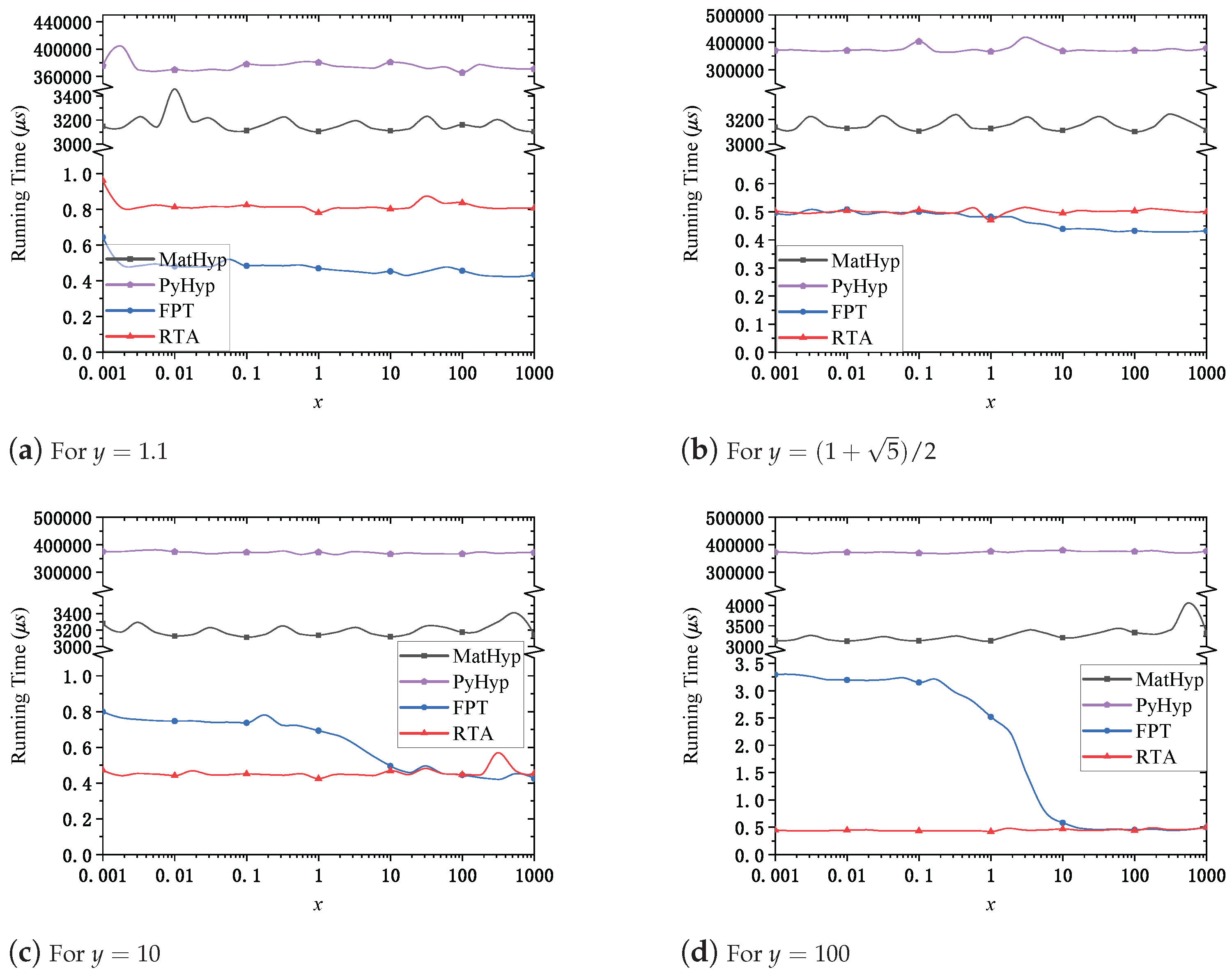
Figure 2 evaluates the runtime behavior of the algorithms as a function of y for representative fixed values of $x\in \{0.1,1,10,100\}$, covering both small and large magnitudes frequently encountered in practical simulations. Both MatHyp and PyHyp serve as reference baselines, consistently exhibiting the higher computational overhead against our method. Specifically, MatHyp requires approximately 3–4 ms per evaluation, while PyHyp incurs an even greater cost, reaching up to 0.4 s. As y increases beyond unity, the runtime of FPT markedly increases, especially pronounced for smaller values of x, revealing FPT’s limited scalability under large-y conditions. In contrast, RTA maintains consistently low runtimes (typically below 1 μs) when y exceeds the threshold value $(1+\sqrt{5})/2$, clearly exhibiting its efficiency and complementary advantage in large-y regimes. The Hybrid algorithm leverages this complementary relationship, dynamically switching between RTA and FPT according to y, thus achieving uniformly stable and minimal runtime across all evaluated conditions. This approach yields speedups of up to ${10}^4\times$, enabling rapid and reliable large-scale simulations. However, it is noted that the relative advantage of RTA diminishes somewhat with increasing x.

Figure 3 investigates runtime performance variations with respect to increasing x at selected fixed values of $y\in \{1.1,(1+\sqrt{5})/2,10,100\}$, again chosen to represent critical operational regimes. MatHyp and PyHyp remain computationally stable but slow across all examined values of x. Notably, RTA consistently demonstrates stable, low, and predictable runtime across the entire range of x, underscoring its robustness. For small x values, RTA consistently surpasses FPT in computational efficiency, an advantage particularly prominent at larger values of y. As x increases, however, the performance gap between RTA and FPT narrows, indicating the diminishing relative benefit of RTA in this regime. The Hybrid algorithm strategically combines the strengths of both methods, selecting the optimal algorithm for each $(x,y)$ pair. This adaptability ensures consistently optimal performance, regardless of the magnitudes of x and y, demonstrating its practical value in adaptive computation scenarios.

Collectively, these experiments validate that RTA consistently achieves rapid convergence and exhibits computational stability, particularly advantageous for large values of y. This comprehensive evaluation clearly highlights the effectiveness and practical value of our proposed approaches in efficiently computing $\Psi (x,y)$.

5.2. Performance in Non-Uniform Cellular Coverage Simulation

To further validate the practical efficacy and accuracy of our proposed Hybrid algorithm, we conduct an in-depth evaluation on SINR coverage calculation within the non-uniform cellular network coverage scenario introduced in Section 3.3. In this context, accurate and rapid computation of the Gauss hypergeometric function $\Psi (x,y)$ is crucial, as it directly appears in interference characterization integral calculations essential to SINR coverage probability assessments. Given the excessive overhead of PyHyp’s performance in Section 5.1, we employ the following three distinct algorithmic settings for comparative analysis: MatHyp: MATLAB’s built-in solver serving as the precise but computationally intensive reference; FPT Only: implemented using only the Pfaff transformation-based algorithm FPT [5]; Hybrid: our proposed Hybrid algorithm as Algorithm 2 which strategically integrates RTA with FPT.

Experimental parameters were meticulously selected to reflect realistic cellular network scenarios. All simulation and numerical analysis parameters, along with their values or sampling ranges, are summarized in

Table 1. Simulation and numerical analysis parameters.

Parameter	Symbol	Value/Range
Deployment radius	R	5
Transmit power scaling	$\mathcal{P}$	1
SINR threshold	q	1
Thermal noise power	$\mathcal{N}$	1
Path-loss exponent	$\eta$	1–5
Average AP density	${\lambda }_0$	1–5
Reliable link probability	P	0–1

for quick reference. Particular emphasis was placed on the path-loss exponent $\eta$ and the average AP density ${\lambda }_0$, which were systematically varied to assess the computational performance of $\Psi$ under different propagation and density conditions. Each $({\lambda }_0,\eta )$ pair involved computing coverage probabilities across uniformly sampled reliable link probabilities P from 0 to 1, with runtime and relative errors averaged as experimental results. 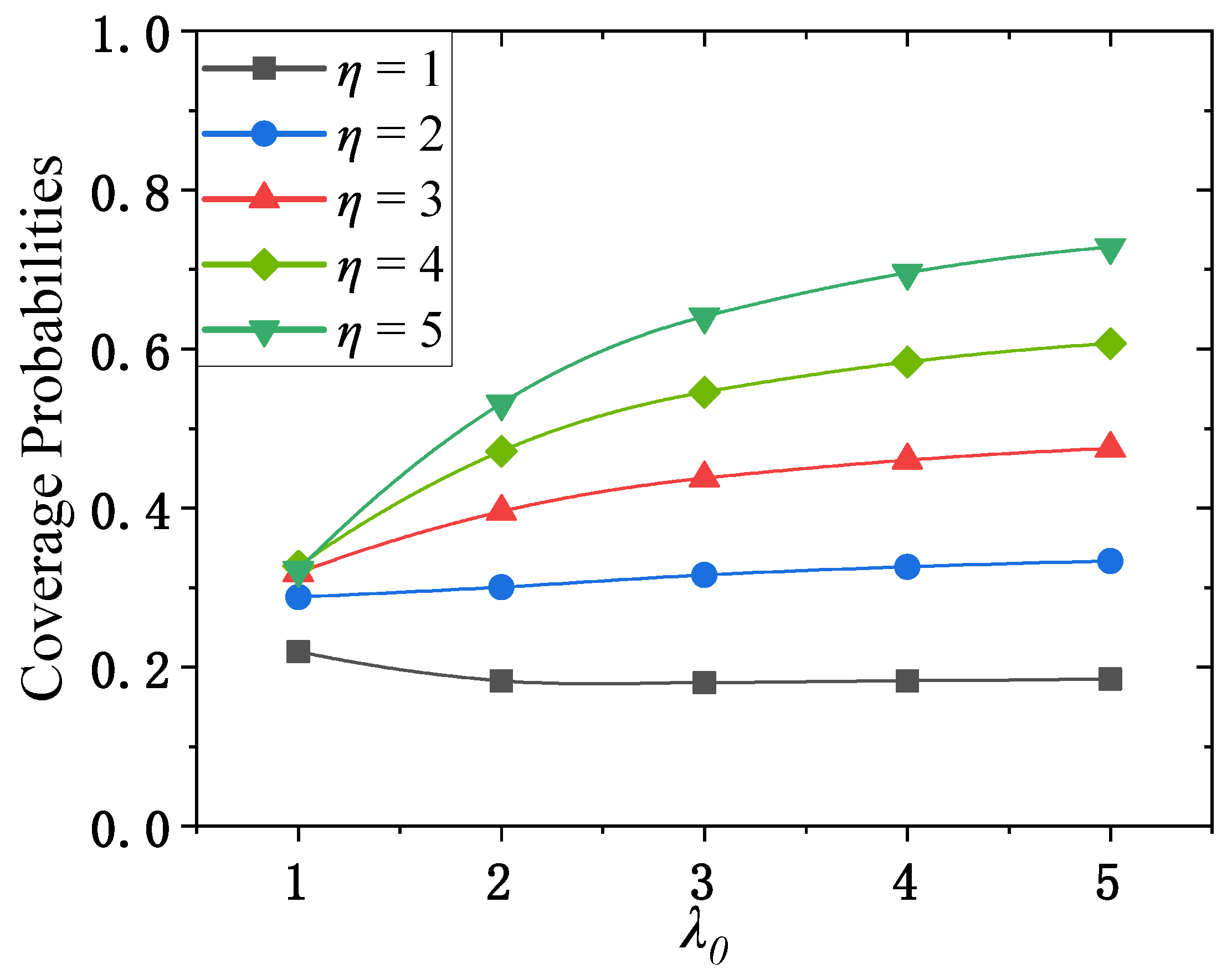In Figure 4, we show the coverage probabilities computed by MatHyp for $P=1$ as the benchmark, which is in line with the work of Pratt et al. [9].

Subsequently, we summarize the accuracy comparison between the FPT Only approach and the proposed Hybrid algorithm, using MatHyp as the accuracy benchmark in

Table 2. Relative error of coverage probability.

Comparison	Max Rel. Error	Mean Rel. Error	Min Rel. Error
FPT Only vs. MatHyp	$4.2\times {10}^{-7}$	$2.6\times {10}^{-8}$	0
Our Hybrid vs. MatHyp	$2.5\times {10}^{-16}$	$2.7\times {10}^{-17}$	0

. Clearly, the Hybrid approach not only substantially enhances computational efficiency but also outperforms FPT Only in numerical precision. Specifically, the Hybrid algorithm maintains relative errors consistently at ${10}^{-16}$, demonstrating nearly perfect fidelity to MatHyp. In contrast, FPT Only exhibits slightly higher maximum relative errors ( $4.2\times {10}^{-7}$), indicating that integrating RTA within the Hybrid framework simultaneously enhances both efficiency and accuracy.

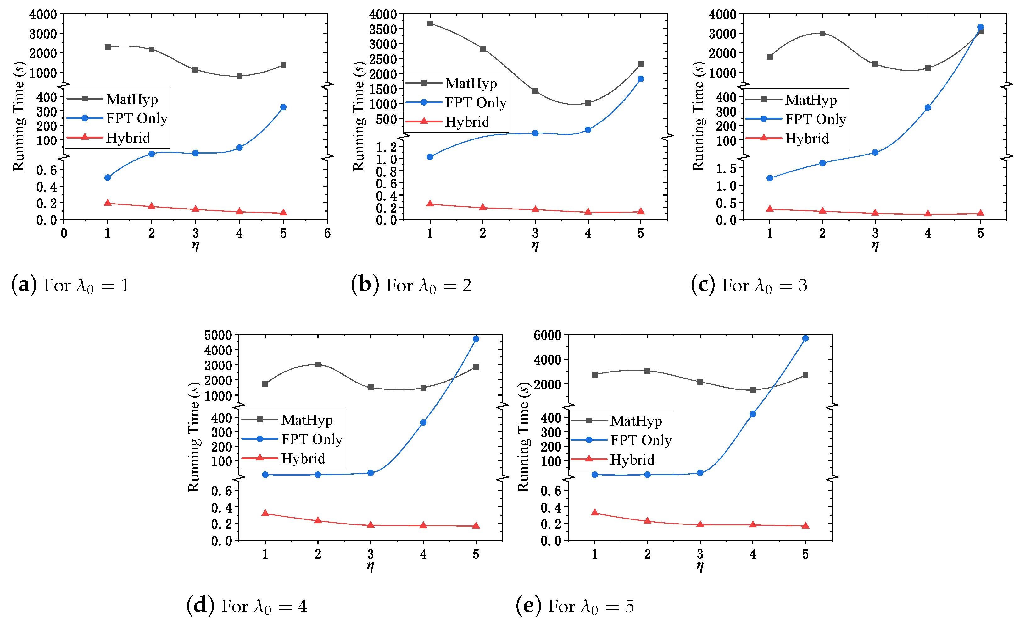
Figure 5 evaluates computational runtime with respect to varying path-loss exponent $\eta$ at fixed AP densities ${\lambda }_0$. MatHyp, although exact, exhibits severe inefficiencies, requiring excessively long computational times that limit practical feasibility in extensive simulation scenarios. The FPT Only improves efficiency significantly over MatHyp but still faces substantial runtime growth at higher $\eta$, indicative of the increased complexity of $\Psi$ evaluation under severe propagation conditions (e.g., Figure 5e, ${\lambda }_0=5$). In sharp contrast, Hybrid displays exceptional computational stability, consistently achieving sub-second runtimes across the full spectrum of $\eta$ values and delivering at least a thousandfold reduction in runtime. This robustness highlights the Hybrid algorithm’s remarkable scalability in handling the direct computational challenges associated with variations in $\eta$.

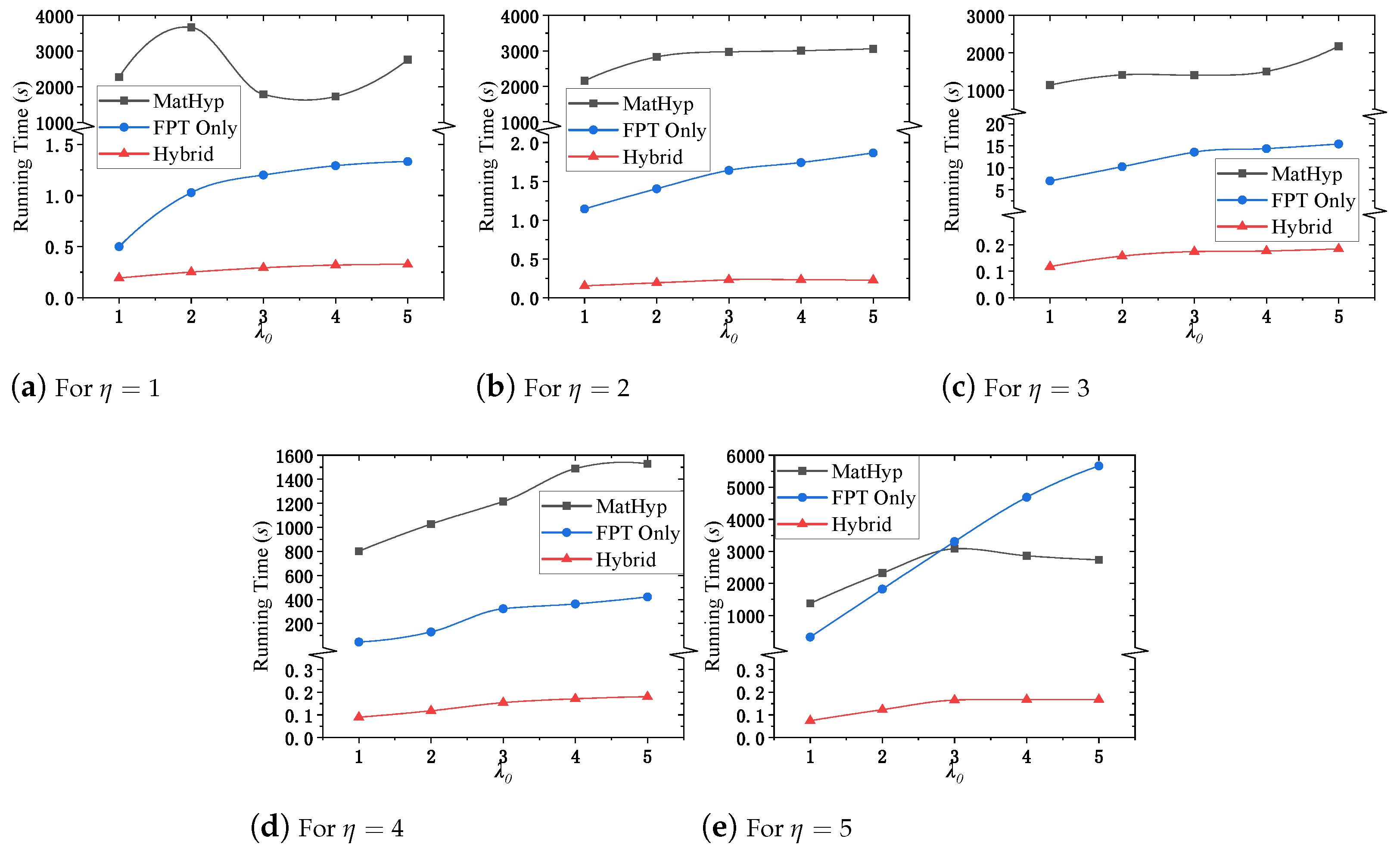
Conversely, Figure 6 provides an alternative perspective by evaluating runtime as a function of AP density ${\lambda }_0$ for fixed $\eta$. Despite ${\lambda }_0$ not directly appearing in the expression of $\Psi$, the increased density indirectly amplifies computational load through more frequent function evaluations and integration complexity. Both built-in and FPT Only methods exhibit significant runtime growth with increasing AP density, especially noticeable in high-$\eta$ cases (e.g., Figure 6e). Remarkably, the Hybrid algorithm remains largely insensitive, maintaining minimal runtime increase even in dense scenarios. This result underscores the Hybrid algorithm’s capability to efficiently manage indirect computational complexities arising from parameter interactions beyond the direct evaluation of $\Psi$.

Collectively, the experimental results above robustly confirm that incorporating our RTA into the Hybrid algorithm markedly improves computational efficiency and numerical precision in SINR coverage probability simulations for non-uniform cellular networks. The substantial runtime reduction, often several orders of magnitude faster than conventional methods, paired with enhanced numerical accuracy, provides compelling evidence supporting the Hybrid algorithm’s applicability in practical large-scale network simulations and real-time optimization frameworks.

6. Conclusions

This paper proposes a highly efficient computational framework for accurately evaluating the zero-balanced Gauss hypergeometric function $\Psi (x,y)$, which serves as a foundational mathematical kernel in various wireless network performance metrics, particularly in non-uniform cellular SINR coverage analyses. By introducing the RTA algorithm, based on a Mellin–Barnes reciprocal-argument identity, we achieve geometric convergence (convergence factor $1/y$) with analytically derived coefficients, thereby circumventing computationally intensive special-function evaluations. Our Hybrid algorithm further integrates this RTA approach with FPT, guided by a precise golden-ratio-based switching criterion, ensuring optimal computational efficiency alongside enhanced numerical precision. Comprehensive experiments confirm that our Hybrid algorithm achieves machine-precision accuracy (errors below ${10}^{-16}$) within 1 μs, substantially outperforming conventional implements in speed and stability. Moreover, realistic SINR coverage evaluations reveal that our Hybrid algorithm dramatically reduced computational time from several hours to mere fractions of a second, demonstrating exceptional scalability in response to direct and indirect complexity factors.

Future work will extend our computational methodology to encompass multivariate hypergeometric functions, which are critically relevant in advanced MIMO interference analyses and ultra-dense network (UDN) scenarios. Meanwhile, drawing inspiration from recent influential studies, including the comprehensive resource allocation strategies and UDN-specific optimizations presented in [23,24,25,26,27], and the pivotal definitions outlined in [23], we will thoroughly incorporate detailed modeling of link reliability, interference effects, multipath fading, shadowing phenomena, and realistic densities of base stations and user equipment. By explicitly comparing coverage probability and SINR results against theoretical predictions, we will validate our computational methods comprehensively. Moreover, implementation-level enhancements, particularly parallelization strategies and GPU acceleration, will be systematically investigated to facilitate hardware-efficient, real-time network optimizations. These future research directions collectively aim to effectively bridge the gap between advanced analytical methodologies and practical communication system designs, laying a robust computational foundation critical for the deployment of next-generation ultra-dense wireless networks.