Bifurcations and Exact Solutions of the Coupled Nonlinear Generalized Zakharov Equations with Anti-Cubic Nonlinearity: Dynamical System Approach

Abstract

We consider the exact traveling wave solutions for the coupled nonlinear generalized Zakharov equations. By employing the method of dynamical systems, we are able to obtain bifurcations of the phase portraits of the corresponding planar dynamical system under various parameter conditions. Based on different level curves, we derive all possible exact explicit parametric representations of bounded solutions, which include pseudo-periodic peakon, pseudo-peakon, smooth periodic wave solutions, solitary solutions, kink wave solution and the compacton solution family.

1. Introduction

Zakharov equations are derived from the standard Zakharov system, a well-established model for describing wave-to-wave interplays in plasmas. Particularly, the coupling between the high-frequency and low-frequency waves is characterized via nonlinear terms, such as the nonlinear term that is proportional to the negative third power of the wave amplitude, the so-called anti-cubic nonlinearity. The anti-cubic nonlinearity is different from the more common cubic nonlinearity discovered in many other wave equations. This actually introduces a unique dynamic where the wave behavior can be significantly affected by small amplitude [1,2]. Recently, the authors in [1] studied the novel exact solutions for the coupled nonlinear generalized Zakharov equations with anti-cubic nonlinearity given by

$$\begin{array}{c}\hfill \begin{array}{cc}\hfill & W_{tt}-c^2{W}_x={\beta \left(\right|E|}^2{)}_x,\hfill \\ \hfill & i{E}_t+\alpha E_{xx}-{\delta }_{1}WE+\left({\displaystyle \frac{{\delta }_0}{{\left|E\right|}^4}}+{\delta }_2{\left|E\right|}^2+{\delta }_3{\left|E\right|}^4\right)E=0,\hfill \end{array}\end{array}$$

(1)

where $c,\beta ,\alpha ,{\delta }_0,{\delta }_1,{\delta }_2$ and ${\delta }_3$ are real constants. Particularly, the parameter c is proportionally linked to ion acoustic speed (or electron sound speed). The function $W=W(x,t)$ portrays the deviation in ion density from its equilibrium state, while $E=E(x,t)$ corresponds to a complex variable symbolizing the slowly changing envelope of the prominently oscillating electronfield. When ${\delta }_0=0,$ the anti-cubic nonlinearity disappears. Furthermore, if ${\delta }_0={\delta }_1={\delta }_2={\delta }_3=0,$ one then has the simplification of the renowned Zakharov system, characterizing the propagation of Langmuir waves in plasma environments.

In order to find the exact solutions of Equation (1), the authors in [1] proposed that the solutions have following form

$$\begin{array}{c}\hfill E(x,t)=\varphi \left(\xi \right)e^{iR(x,t)},W(x,t)=W\left(\xi \right),\xi =x-vt,R(x,t)=-\kappa x-\omega t+\theta \left(\xi \right),\end{array}$$

(2)

where $v,\kappa$ and $\omega$ are constant parameters. Substituting the assumption (2) into the Equation (1), decomposing into real and imaginary parts, and integrating the obtained equations, the authors in [1] obtained

$$\begin{array}{c}\hfill \begin{array}{cc}\hfill & \alpha {\varphi }^{″}+\left(\omega +v\kappa +{\displaystyle \frac{v^2}{4\alpha }}\right)\varphi +\left({\delta }_0-{\displaystyle \frac{c_0^2}{\alpha }}\right){\varphi }^{-3}+\left({\delta }_2-{\displaystyle \frac{\beta {\delta }_1}{v^2-c^2}}\right){\varphi }^3+{\delta }_3{\varphi }^5=0,\hfill \\ \hfill & W\left(\xi \right)=\left({\displaystyle \frac{\beta }{v^2-c^2}}\right){\varphi }^2\left(\xi \right),\hfill \\ \hfill & \theta \left(\xi \right)={\displaystyle \frac{k_0}{\alpha }}\int {\displaystyle \frac{d\xi }{{\varphi }^2\left(\xi \right)}}+\left({\displaystyle \frac{v+2\alpha \kappa }{2\alpha }}\right)\xi ,\hfill \end{array}\end{array}$$

(3)

where $k_0$ is an integral constant.

To get started for our study, we first introduce

$$a_1={\displaystyle \frac{1}{\alpha }}\left(\omega +v\kappa +{\displaystyle \frac{v^2}{4\alpha }}\right),a_3={\displaystyle \frac{1}{\alpha }}\left({\delta }_2-{\displaystyle \frac{\beta {\delta }_1}{v^2-c^2}}\right),a_5={\displaystyle \frac{{\delta }_3}{\alpha }},b={\displaystyle \frac{1}{\alpha }}\left({\delta }_0-{\displaystyle \frac{c_0^2}{\alpha }}\right).$$

Then, the first equation in (3) is equivalent to the following planar Hamiltonian system

$$\begin{array}{c}\hfill \begin{array}{cc}\hfill & {\displaystyle \frac{d\varphi }{d\xi }}=y,\hfill \\ \hfill & {\displaystyle \frac{dy}{d\xi }}={\displaystyle \frac{b+{\varphi }^4(a_1+a_3{\varphi }^2+a_5{\varphi }^4)}{{\varphi }^3}}\hfill \end{array}\end{array}$$

(4)

with the first integral given by

$$\begin{array}{c}\hfill H_0(\varphi ,y)={\displaystyle \frac{1}{2}}{y}^2-{\displaystyle \frac{1}{2}}{a}_1{\varphi }^2-{\displaystyle \frac{1}{4}}{a}_3{\varphi }^4-{\displaystyle \frac{1}{6}}{a}_5{\varphi }^6+{\displaystyle \frac{b}{2{\varphi }^2}}:=h.\end{array}$$

(5)

Note that $H_0(-\varphi ,y)=H_0(\varphi ,y).$ The level curves defined by $H_0(\varphi ,y)=h$ are symmetry with respect to the $y-$axis. Correspondingly, we will only discuss the phase portraits in the right half-phase plane for the system (4).

We would like to point out that the authors in [1] introduced the transformation $\varphi ={\left(g\left(\xi \right)\right)}^{{\displaystyle \frac{1}{2}}}$ for their analysis. With this transformation, the system (4) becomes

$$\begin{array}{c}\hfill {\displaystyle \frac{dg}{d\xi }}=y,{\displaystyle \frac{dy}{d\xi }}={\displaystyle \frac{-y^2+4b+4g^2(a_1+a_{3}g+a_5{g}^2)}{2g}}\end{array}$$

(6)

with the first integral

$$\begin{array}{c}\hfill H(g,y)=y^{2}g-g\left(4b+{\displaystyle \frac{4}{3}}{a}_1{g}^2+a_3{g}^3+{\displaystyle \frac{4}{5}}{a}_5{g}^4\right)=h.\end{array}$$

(7)

Unfortunately, the authors in [1] did not derive the system (6) and the integral (7). On the other hand, if we just consider the first integral $H_0(\varphi ,y)=h$ given by (5), then, with the transformation $\varphi ={\left(g\left(\xi \right)\right)}^{{\displaystyle \frac{1}{2}}}$, the first integral (5) becomes

$$\begin{array}{c}\hfill H_0(g,y)={\displaystyle \frac{1}{2}}{y}^2-{\displaystyle \frac{1}{2}}{a}_{1}g-{\displaystyle \frac{1}{4}}{a}_3{g}^2-{\displaystyle \frac{1}{6}}{a}_5{g}^3+{\displaystyle \frac{b}{2g}}=h.\end{array}$$

(8)

Clearly, the first integral (8) is different from the first integral (7). Furthermore, we point out that the formula (2.13) in [1] is not correct. Therefore, the results obtained in [1] need to be corrected. Meanwhile, we emphasize that for an integrable planar differential system, if one makes a variable transformation, the corresponding new equation with respect to the new variable must be derived, and the new first integral must be found. To correct this mistake and provide a comprehensive understanding of the underlying problem is the main motivation of this work.

In the past three decades, nonlinear wave equations with non-smooth solitary wave solution called peakon and periodic peakon and the solution family having compact support called compactons (see [3]) have attracted a lot of attention. Peakon was first coined by the authors in [4,5,6], and thereafter other peakon equations were developed (see [7,8,9,10,11,12,13] and references therein). In this work, we directly consider the system (4), which is a four-parameter system depending on the parameter group $(b,a_1,a_3,a_5)$. Clearly, the system (4) is a singular traveling wave system of the first kind defined by the authors in [14,15] with the singular straight line $\varphi =0.$ We will apply the method of dynamical systems [16,17,18,19,20,21,22] to discuss the dynamical behavior of solutions $\varphi \left(\xi \right)$, and under different parameter conditions to find exact solutions of the system (4). The approach we take is different from the various techniques employed in [1]. Our main result is stated as follows:

Theorem 1. 

For the coupled nonlinear generalized Zakharov Equations (1), One has

(i) 

The system (4) has the traveling wave solutions given by

$$\begin{array}{c}\hfill \begin{array}{cc}\hfill & E(x,t)=\sqrt{\psi \left(\xi \right)}{e}^{i(-\kappa x-\omega t+\theta (\xi \left)\right)},\xi =x-vt,\hfill \\ \hfill & W(x,t)={\displaystyle \frac{\beta \psi \left(\xi \right)}{v^2-c^2}},\hfill \\ \hfill & \theta \left(\xi \right)={\displaystyle \frac{k_0}{\alpha }}\int {\displaystyle \frac{d\xi }{\psi \left(\xi \right)}}+\left({\displaystyle \frac{v+2\alpha \kappa }{2\alpha }}\right)\xi ,\hfill \end{array}\end{array}$$

(9)

where $\psi \left(\xi \right)={\left(\varphi \left(\xi \right)\right)}^2$, and $\varphi \left(\xi \right)$ satisfies the planar dynamical system (4).

(ii) 

Under different parameter conditions, the system (4) has the bifurcations of phase portraits which are shown in Figure 1, Figure 2, Figure 3 and Figure 4.

(iii) 

$\psi \left(\xi \right)$ has explicit exact solutions given by (14)–(36).

Figure 1. Bifurcations of the phase portraits of the system (4) with $a_5>0$.

Figure 2. Bifurcations of the phase portraits of the system (4) with $a_5<0$.

Figure 3. Bifurcations of the phase portraits of the system (4) with $F\left(\psi \right)=0$ has two positive roots.

Figure 4. Bifurcations of the phase portraits of the system (4) with $F\left(\psi \right)=0$ has one positive root.

The article is organized as follows. In Section 2, we discuss the bifurcations of phase portraits for the systems (4). In Section 3, Section 4 and Section 5, we derive all possible exact explicit parametric representations for some bounded solutions of the system (4), while Section 6 is a concluding remark.

2. Bifurcations of Phase Portraits of the System (4)

In this section, we focus on the associated regular system of the system (4), which is given by

$$\begin{array}{c}\hfill \begin{array}{cc}\hfill & {\displaystyle \frac{d\psi }{d\zeta }}={\varphi }^{3}y,\hfill \\ \hfill & {\displaystyle \frac{dy}{d\zeta }}=b+{\varphi }^4(a_1+a_3{\varphi }^2+a_5{\varphi }^4),\hfill \end{array}\end{array}$$

(10)

where $d\xi ={\varphi }^{3}d\zeta$. For $\psi \ne 0,$ this system has the same first integral as that of the system (4). The dynamics of the system (4) and the system (10) are different in the neighborhood of the straight line $\varphi =0$. Specially, under some parameter conditions, the variable $\zeta$ is a fast variable while the variable $\xi$ is a slow variable in the sense of the geometric singular perturbation theory.

Let $F\left(\psi \right)=b+{\psi }^{2}f\left(\psi \right)$ and $f\left(\psi \right)=a_1+a_3\psi +a_5{\psi }^2,$ where $\psi ={\varphi }^2$. We have

$$F^{\prime }\left(\psi \right)=(2a_1+3a_3\psi +4a_5{\psi }^2)\psi .$$

It is easy to see that $F^{\prime }\left(\psi \right)=0$ has three real roots:

$${\psi }_0=0,{\psi }_1={\displaystyle \frac{-3a_3-\sqrt{\Delta }}{8a_5}}and{\psi }_2={\displaystyle \frac{-3a_3+\sqrt{\Delta }}{8{\alpha }_5}},$$

where $\Delta =9a_3^2-32a_1{a}_5\ge 0.$ Direct calculation gives

$$\begin{array}{c}\hfill F\left({\psi }_1\right)={\displaystyle \frac{1}{512a_5^3}}\left[-128a_1^2{a}_5^2+144a_1{a}_3^2{a}_5-27a_3^4+512b{a}_5^3+(32a_1{a}_3{a}_5-9a_3^3)\sqrt{\Delta }\right]\end{array}$$

(11)

and

$$\begin{array}{c}\hfill F\left({\psi }_2\right)=-{\displaystyle \frac{1}{512a_5^3}}\left[128a_1^2{a}_5^2-144a_1{a}_3^2{a}_5+27a_3^4-512b{a}_5^3+(32a_1{a}_3{a}_5-9a_3^3)\sqrt{\Delta }\right].\end{array}$$

(12)

Let $z_j$ be a positive real root of $F\left(\psi \right)=0$, one can check directly that in the positive $\varphi -$axis of the phase plane, the system (10) has an equilibrium point $E_j(\sqrt{z_j},0).$ Furthermore, we have the following facts, which are fundamental for our later analysis.

(i)

If $a_1{a}_5>0,a_3{a}_5<0$ and $\Delta >0,$ then $F^{\prime }\left(\psi \right)$ has two positive real zeros. Furthermore,

(i1)

If $b{a}_5<0,$ $F\left({\psi }_1\right)>0$ and $F\left({\psi }_2\right)<0,$ then $F\left(\psi \right)$ has three positive real zeros $z_j(j=1,2,3)$ satisfying $0<z_1<{\psi }_1<z_2<{\psi }_2<z_3$ for ${\alpha }_5>0$ and $0<z_1<{\psi }_2<z_2<{\psi }_1<z_3$ for $a_5<0$.

(i2)

If $b{a}_5<0,$ and either $F\left({\psi }_1\right)=0$ or $F\left({\psi }_2\right)=0,$ then $F\left(\psi \right)$ has a double positive real zero.

(i3)

If $b{a}_5>0,$ and $a_{5}F\left({\psi }_j\right)<0,j=1,2$, then $F\left(\psi \right)$ has two positive real zeros $z_j(j=1,2)$ satisfying $0<{\psi }_1<z_1<{\psi }_2<z_2$ for $a_5>0$ and $0<{\psi }_2<z_1<{\psi }_1<z_2$ for $a_5<0$.

(ii)

When $\Delta <0,$ if $b{a}_5<0,$ then $F\left(\psi \right)$ has an positive real zero.

Let $M({\varphi }_j,0)$ be the coefficient matrix of the linearized system of the system (10) at an equilibrium point $E_j({\varphi }_j,0)$ with ${\varphi }_j=\sqrt{z_j}$, and $J({\varphi }_j,0)=\det \mathrm{M}({\varphi }_j,0)$. We have

$$J({\varphi }_j,0)=-2{\varphi }_j^6{f}^{\prime }\left(z_j\right).$$

Let $h_j=H_0({\varphi }_j,0),$ where $H_0$ is given by (5). Based on the above information, we are ready for our qualitative analysis of the problem. We first have the following bifurcations of the phase portraits of the system (4) shown in Figure 1, Figure 2, Figure 3 and Figure 4.

(I)

The case that there exist three equilibrium points (including double points) of the system (4) in the positive $\varphi -$axis.

(II)

The case that there exist two equilibrium points (including double points) of the system (4) in the positive $\varphi -$axis.

(III)

The case that there exists one equilibrium point of the system (4) in the positive $\varphi -$axis.

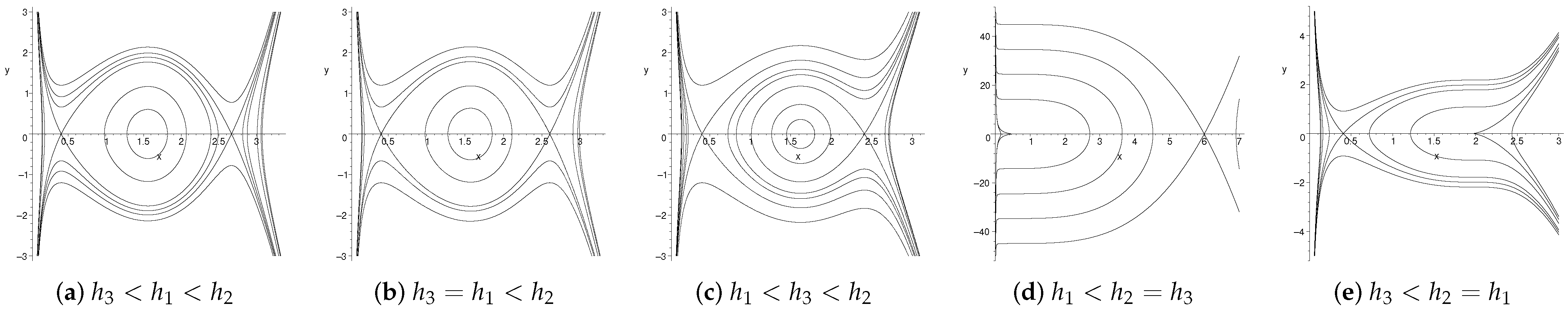
3. Explicit Exact Parametric Representations of the Solutions of the System (4) with Three Equilibrium Points and a₅ >0

It is known that for a given real number h, the function $H_0(\varphi ,y)=h$ given by (5) defines level curves of the system (4), which can have different branches. We see from (4) that

$$y^2={\displaystyle \frac{1}{{\varphi }^2}}(-b+2h{\varphi }^2+{\alpha }_1{\varphi }^4+{\displaystyle \frac{1}{2}}{\alpha }_3{\varphi }^6+{\displaystyle \frac{1}{3}}{\alpha }_5{\varphi }^8).$$

Hence, by using the first equation of the system (4), we obtain

$$\begin{array}{c}\hfill \begin{array}{cc}\hfill \xi =& {\int }_{{\varphi }_0}^{\varphi }{\displaystyle \frac{\varphi d\varphi }{\sqrt{|-b+2h{\varphi }^2+a_1{\varphi }^4+\frac{1}{2}{a}_3{\varphi }^6+\frac{1}{3}{a}_5{\varphi }^8|}}}\hfill \\ \hfill =& {\int }_{{\psi }_0}^{\psi }{\displaystyle \frac{d\psi }{2\sqrt{|-b+2h\psi +a_1{\psi }^2+\frac{1}{2}{a}_3{\psi }^3+\frac{1}{3}{a}_5{\psi }^4|}}},\hfill \end{array}\end{array}$$

(13)

where $\psi ={\varphi }^2.$ By using (13), we can calculate the parametric representations of $\varphi \left(\xi \right)=\sqrt{\psi \left(\xi \right)}$ of the orbits of the system (4). Because of $\varphi =\sqrt{\psi },$ we only need to find the solutions of $\psi \left(\xi \right)>0.$ More precisely, we use (13) to calculate the explicit exact parametric representations $\varphi \left(\xi \right)=\sqrt{\psi \left(\xi \right)}$ of solutions of the system (4) for the case that there exist three equilibrium points and $a_5>0$.

3.1. The Parametric Representations of the Bounded Orbits Given by Figure 1a

In Figure 1a, as h is varied, the changes of level curves defined by $H_0(\varphi ,y)=h$ are shown in Figure 5, from case (a) to case (e).

Figure 5. The change of level curves defined by $H_0(\varphi ,y)=h$ in the case (a) of Figure Section 1.

Next, we only consider the level curves in the right phase plane due to the symmetry as discussed above.

(i)

Corresponding to the level curves defined by $H_0(\varphi ,y)=h$ with $h\in (-\infty ,h_2)$, there exist two families of open orbits of the system (4), for which one family tends to the singular straight line $\varphi =0$, when $\left|y\right|\to \infty$ (see Figure 5a). This open orbit family gives rise to a family of compacton solutions. Correspondingly, (13) can be written as

$$\sqrt{{\displaystyle \frac{4a_5}{3}}}\xi ={\int }_{\psi }^{{\psi }_b}{\displaystyle \frac{d\psi }{\sqrt{({\psi }_a-\psi )({\psi }_b-\psi )[{(\psi -{\widehat{b}}_1)}^2+{\widehat{a}}_1^2]}}},$$

from which we obtain the parametric representation of the family of compacton solutions given by

$$\begin{array}{c}\hfill \psi \left(\xi \right)={\displaystyle \frac{({\psi }_a{B}_1+{\psi }_b{A}_1)-({\psi }_a{B}_1-{\psi }_b{A}_1)cn({\Omega }_1\xi ,k))}{(A_1+B_1)+(A_1-B_1)cn({\Omega }_1\xi ,k)}},\xi \in (-{\xi }_{01},{\xi }_{01}).\end{array}$$

(14)

Here

$$\begin{array}{cc}\hfill A_1^2=& {({\psi }_a-{\widehat{b}}_1)}^2+{\widehat{a}}_1^2,B_1^2={({\psi }_b-{\widehat{b}}_1)}^2+{\widehat{a}}_1^2,k^2={\displaystyle \frac{{({\psi }_a-{\psi }_b)}^2-{(A_1-B_1)}^2}{4A_1{B}_1}},\hfill \\ \hfill {\Omega }_1=& \sqrt{{\displaystyle \frac{4a_5{A}_1{B}_1}{3}}},{\xi }_{01}={\displaystyle \frac{1}{{\Omega }_1}}c{n}^{-1}\left({\displaystyle \frac{{\psi }_a{B}_1+{\psi }_b{A}_1}{{\psi }_a{B}_1-{\psi }_b{A}_1}}\right),\hfill \end{array}$$

where $sn(·,k),cn(·,k),dn(·,k)$ are the Jacobin elliptic functions (see [23]).

(ii)

Corresponding to the level curves defined by $H_0(\varphi ,y)=h$ with $h\in (h_2,h_1),$ there exists a family of periodic orbits and two families of open orbits of the system (4) (see Figure 5b). For the family of periodic orbits, (13) can be written as

$$\sqrt{{\displaystyle \frac{4a_5}{3}}}\xi ={\int }_{{\psi }_c}^{\psi }{\displaystyle \frac{d\psi }{\sqrt{({\psi }_a-\psi )({\psi }_b-\psi )(\psi -{\psi }_c)(\psi -{\psi }_d)}}},$$

from which we obtain the parametric representation of the family of periodic solutions of the system (4) given by

$$\begin{array}{c}\hfill \psi \left(\xi \right)={\psi }_d+{\displaystyle \frac{{\psi }_c-{\psi }_d}{1-{\widehat{\alpha }}_1^2{\mathrm{sn}}^2({\Omega }_2\xi ,k)}},\end{array}$$

(15)

where

$${\widehat{\alpha }}_1^2={\displaystyle \frac{{\psi }_b-{\psi }_c}{{\psi }_b-{\psi }_d}},k^2={\displaystyle \frac{{\widehat{\alpha }}_1^2({\psi }_a-{\psi }_d)}{{\Psi }_a-{\psi }_c}}\mathrm{and}{\Omega }_2=\sqrt{{\displaystyle \frac{a_5({\psi }_a-{\psi }_c)({\psi }_b-{\psi }_d)}{3}}}.$$

Recall from (9) that $\theta \left(\xi \right)={\displaystyle \frac{k_0}{\alpha }}\int {\displaystyle \frac{d\xi }{\psi \left(\xi \right)}}+\left({\displaystyle \frac{v+2\alpha \kappa }{2\alpha }}\right)\xi$. For $\psi \left(\xi \right)$ given by (15), one has

$$\begin{array}{cc}\hfill \int {\displaystyle \frac{d\xi }{\psi \left(\xi \right)}}& ={\displaystyle \frac{1}{{\psi }_c}}\int {\displaystyle \frac{1}{1-\frac{{\psi }_d{\widehat{\alpha }}_1^2}{{\psi }_c}{\mathrm{sn}}^2({\Omega }_2\xi ,k)}}-{\displaystyle \frac{{\widehat{\alpha }}_1^2{\mathrm{sn}}^2({\Omega }_2\xi ,k)}{1-\frac{{\psi }_d{\widehat{\alpha }}_1^2}{{\psi }_c}{\mathrm{sn}}^2({\Omega }_2\xi ,k)}}d\psi \hfill \\ \hfill & =\left({\displaystyle \frac{1}{{\psi }_c}}-{\displaystyle \frac{1}{{\psi }_d}}\right)\Pi \left(arcsin(\mathrm{sn}({\Omega }_2\xi ,k),{\displaystyle \frac{{\psi }_d{\widehat{\alpha }}_1^2}{{\psi }_c}},k\right)-{\displaystyle \frac{1}{{\psi }_d}}F\left(arcsin(\mathrm{sn}({\Omega }_2\xi ,k),k\right),\hfill \end{array}$$

where $F(·,k)$ is the elliptic integral of first kind, and $\Pi (·,·,k)$ is the elliptic integral of third kind. It follows that for known $\psi \left(\xi \right)$ given by (15), we obtain

$$\begin{array}{c}\hfill \begin{array}{cc}\hfill \theta \left(\xi \right)& :={\theta }_1\left(\xi \right)={\displaystyle \frac{v+2\alpha \kappa }{2\alpha }}\xi +{\displaystyle \frac{k_0}{\alpha }}\left[\left({\displaystyle \frac{1}{{\psi }_c}}-{\displaystyle \frac{1}{{\psi }_d}}\right)\Pi \left(arcsin(\mathrm{sn}({\Omega }_2\xi ,k),{\displaystyle \frac{{\psi }_d{\widehat{\alpha }}_1^2}{{\psi }_c}},k\right)\right.\hfill \\ \hfill & \left.-{\displaystyle \frac{1}{{\psi }_d}}F\left(arcsin(\mathrm{sn}({\Omega }_2\xi ,k),k\right)\right].\hfill \end{array}\end{array}$$

(16)

For the family of open orbits which tend to the singular straight line $\varphi =0$ as $\left|y\right|\to \infty$, (13) can be written as

$$\sqrt{{\displaystyle \frac{4a_5}{3}}}\xi ={\int }_{\psi }^{{\psi }_d}{\displaystyle \frac{d\psi }{\sqrt{({\psi }_a-\psi )({\psi }_b-\psi )({\psi }_c-\psi )({\psi }_d-\psi )}}},$$

from which we have the following compacton solution family of the system (4):

$$\begin{array}{c}\hfill \psi \left(\xi \right)={\psi }_c-{\displaystyle \frac{{\psi }_c-{\psi }_d}{1-{\widehat{\alpha }}_2^2\mathrm{s}{\mathrm{n}}^2({\Omega }_2\xi ,k)}},\xi \in (-{\xi }_{02},{\xi }_{02}),\end{array}$$

(17)

where

$$\begin{array}{cc}\hfill & {\widehat{\alpha }}_2^2={\displaystyle \frac{{\psi }_a-{\psi }_d}{{\psi }_a-{\psi }_c}},k^2={\displaystyle \frac{{\widehat{\alpha }}_2^2({\psi }_b-{\psi }_c)}{{\psi }_b-{\psi }_d}},\hfill \\ \hfill & {\Omega }_2=\sqrt{{\displaystyle \frac{a_5({\psi }_a-{\psi }_c)({\psi }_b-{\psi }_d)}{3}}},{\xi }_{02}={\displaystyle \frac{1}{{\Omega }_2}}\mathrm{s}{\mathrm{n}}^{-1}\sqrt{{\displaystyle \frac{{\psi }_d}{{\widehat{\alpha }}_2^2{\psi }_c}}}.\hfill \end{array}$$

(iii)

The level curves defined by $H(\varphi ,y)=h_1$ contain a homoclinic orbit to the equilibrium point $E_1({\varphi }_1,0)$ and an open orbit (see Figure 5c). For the homoclinic orbit enclosing the equilibrium point $E_2({\varphi }_2,0)$, (13) can be written as

$$\sqrt{{\displaystyle \frac{4a_5}{3}}}\xi ={\int }_{\psi }^{{\psi }_M}{\displaystyle \frac{d\psi }{(\psi -{\psi }_1)\sqrt{({\psi }_L-\psi )({\psi }_M-\psi )}}},$$

from which one has the parametric representation of a solitary wave solution of the system (4)

$$\begin{array}{c}\hfill \psi \left(\xi \right)={\psi }_1+{\displaystyle \frac{2({\psi }_L-{\psi }_1)({\psi }_M-{\psi }_1)}{({\psi }_L-{\psi }_M)cosh\left({\omega }_1\xi \right)+({\psi }_L+{\psi }_M-2{\psi }_1)}},\end{array}$$

(18)

where ${\omega }_1=\sqrt{{\displaystyle \frac{4}{3}}{a}_5({\psi }_L-{\psi }_1)({\psi }_M-{\psi }_1)}.$ For the $\psi \left(\xi \right)$ given by (18), let

$$\begin{array}{cc}\hfill A_0=& ({\psi }_L-{\psi }_1)({\psi }_M-{\psi }_1),B_0=({\psi }_L+{\psi }_M-2{\psi }_1),\hfill \\ \hfill {\widehat{A}}_0=& \sqrt{{(B_0+{\displaystyle \frac{2A_0}{{\psi }_1}})}^2-{({\psi }_L-{\psi }_M)}^2},{\widehat{B}}_0=B_0+{\displaystyle \frac{2A_0}{{\psi }_1}}+({\psi }_L-{\psi }_M),\hfill \end{array}$$

one has

$$\begin{array}{cc}\hfill \int {\displaystyle \frac{d\xi }{\psi \left(\xi \right)}}& ={\displaystyle \frac{\xi }{{\psi }_1}}-{\displaystyle \frac{2A_0}{{\psi }_1^2}}\int {\displaystyle \frac{d\xi }{({\psi }_L-{\psi }_M)cosh\left({\omega }_1\xi \right)+B_0+\frac{2A_0}{{\psi }_1}}}\hfill \\ \hfill & ={\displaystyle \frac{\xi }{{\psi }_1}}-{\displaystyle \frac{2A_0}{{\psi }_1^2{\omega }_1{\widehat{A}}_0}}ln\left({\displaystyle \frac{{\widehat{B}}_0+{\widehat{A}}_{0}tanh\left(\frac{1}{2}{\omega }_1\xi \right)}{{\widehat{B}}_0-{\widehat{A}}_{0}tanh\left(\frac{1}{2}{\omega }_1\xi \right)}}\right).\hfill \end{array}$$

It follows that

$$\begin{array}{c}\hfill \theta \left(\xi \right)={\theta }_2\left(\xi \right)=\left({\displaystyle \frac{v+2\alpha \kappa }{2\alpha }}+{\displaystyle \frac{1}{{\psi }_1}}\right)\xi -{\displaystyle \frac{2k_0{A}_0}{\alpha {\psi }_1^2{\omega }_1{\widehat{A}}_0}}ln\left({\displaystyle \frac{{\widehat{B}}_0+{\widehat{A}}_{0}tanh\left(\frac{1}{2}{\omega }_1\xi \right)}{{\widehat{B}}_0-{\widehat{A}}_{0}tanh\left(\frac{1}{2}{\omega }_1\xi \right)}}\right).\end{array}$$

(19)

(iv)

The level curves defined by $H_0(\varphi ,y)=h$ with $h\in (h_3,h_1)$ are two open curve families, for which one curve family tends to the singular straight line $\varphi =0$ as $\left|y\right|\to \infty$. It gives rise to a compacton solution family having the same parametric representation as that of (14).

(v)

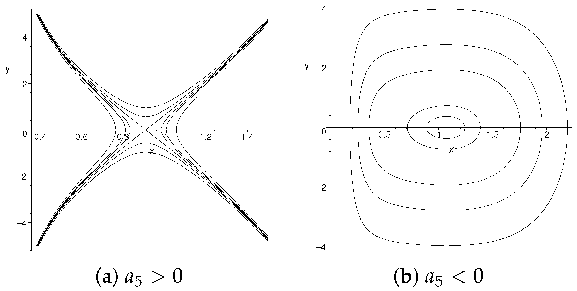
The level curves defined by $H_0(\varphi ,y)=h_3$ are two stable manifolds and two unstable manifolds of the saddle point $E_3({\varphi }_3,0)$, for which two manifolds tend to the singular straight line $\varphi =0$ as $\left|y\right|\to \infty$ (see Figure 5e). For the left stable manifold, (13) can be written as

$$\begin{array}{cc}\hfill \sqrt{{\displaystyle \frac{4a_5}{3}}}\xi =& {\int }_0^{\psi }{\displaystyle \frac{d\psi }{({\psi }_3-\psi )\sqrt{a_0+b_0\psi +{\psi }^2}}}\hfill \\ \hfill =& {\int }_{\tilde{\psi }}^{{\psi }_3}{\displaystyle \frac{d\tilde{\psi }}{\tilde{\psi }\sqrt{(a_0+b_0{\psi }_3+{\psi }_3^2)-(b_0+2{\psi }_3)\tilde{\psi }+{\tilde{\psi }}^2}}},\hfill \\ \hfill {\Delta }_0=& b_0^2-4a_0<0,\hfill \end{array}$$

from which one has the following parametric representation of the stable manifold

$$\begin{array}{c}\hfill \psi \left(\xi \right)={\displaystyle \frac{2(a_0+b_0{\psi }_3+{\psi }_3^2)}{\sqrt{-{\Delta }_0}sinh({\omega }_2\xi +{\widehat{\xi }}_0)+(b_0+2{\psi }_3)}},\end{array}$$

(20)

where ${\omega }_2=\sqrt{{\displaystyle \frac{4a_5}{3}}(a_0+b_0{\psi }_3+{\psi }_3^2)}$ and ${\widehat{\xi }}_0={sinh}^{-1}\left({\displaystyle \frac{2a_0+b_0{\psi }_3}{{\psi }_3\sqrt{-{\Delta }_0}}}\right).$

3.2. The Parametric Representations of the Heteroclinic Orbits Given by Figure 1b

The level curves defined by $H_0(\varphi ,y)=h_1=h_3$ contain two heteroclinic orbits connecting the two equilibrium points $E_1({\varphi }_1,0)$ and $E_3({\varphi }_3,0)$, and the stable manifolds and unstable manifolds of these saddle points. For the above heteroclinic orbit, (13) can be written as

$$\sqrt{{\displaystyle \frac{4a_5}{3}}}\xi ={\int }_{{\psi }_2}^{\psi }{\displaystyle \frac{d\psi }{({\psi }_3-\psi )(\psi -{\psi }_1)}},$$

from which one has the parametric representation of the the kink wave solution of the system (4):

$$\begin{array}{c}\hfill \psi \left(\xi \right)={\psi }_3-{\displaystyle \frac{{\psi }_3-{\psi }_1}{1+m_0{e}^{{\omega }_3\xi }}},\end{array}$$

(21)

where $m_0={\displaystyle \frac{{\psi }_2-{\psi }_1}{{\psi }_3-{\psi }_2}}$ and ${\omega }_3=\sqrt{{\displaystyle \frac{1}{3}}{a}_5({\psi }_3-{\psi }_1)}.$ For $\psi \left(\xi \right)$ given by (21), we have

$$\begin{array}{cc}\hfill \int {\displaystyle \frac{d\xi }{\psi \left(\xi \right)}}=& {\displaystyle \frac{\xi }{{\psi }_3}}+({\psi }_3-{\psi }_1)\int {\displaystyle \frac{d\xi }{m_0{\psi }_3{e}^{{\omega }_3\xi }-{\psi }_1}}\hfill \\ \hfill =& {\displaystyle \frac{\xi }{{\psi }_3}}+{\displaystyle \frac{({\psi }_3-{\psi }_1)}{{\omega }_3{\psi }_1}}ln\left(m_0{\psi }_3-{\psi }_1{e}^{-{\omega }_3\xi }\right).\hfill \end{array}$$

It follows that

$$\begin{array}{c}\hfill \theta \left(\xi \right)={\theta }_3\left(\xi \right)=\left({\displaystyle \frac{v+2\alpha \kappa }{2\alpha }}+{\displaystyle \frac{1}{{\psi }_3}}\right)\xi +{\displaystyle \frac{k_0({\psi }_3-{\psi }_1)}{\alpha {\omega }_3{\psi }_1}}ln\left(m_0{\psi }_3-{\psi }_1{e}^{-{\omega }_3\xi }\right).\end{array}$$

(22)

3.3. The Parametric Representations of the Homoclinic Orbit Given by Figure 1c

The level curves defined by $H_0(\varphi ,y)=h_3$ contain a homoclinic orbit to the equilibrium point $E_3({\varphi }_3,0)$ and an open orbit which tends to the singular straight line $\varphi =0$ as $\left|y\right|\to \infty$ and passes through the point $({\varphi }_l,0)$. For the homoclinic orbit, (13) can be written as

$$\sqrt{{\displaystyle \frac{4a_5}{3}}}\xi ={\int }_{{\psi }_m}^{\psi }{\displaystyle \frac{d\psi }{({\psi }_3-\psi )\sqrt{(\psi -{\psi }_m)(\psi -{\psi }_1)}}},$$

from which one has the parametric representation of a solitary wave solution of the system (4)

$$\begin{array}{c}\hfill \psi \left(\xi \right)={\psi }_3-{\displaystyle \frac{2({\psi }_3-{\psi }_m)({\psi }_3-{\psi }_l)}{({\psi }_m-{\psi }_l)cosh\left({\omega }_4\xi \right)+(2{\psi }_3-{\psi }_m-{\psi }_l)}},\end{array}$$

(23)

where ${\omega }_4=\sqrt{{\displaystyle \frac{4}{3}}{a}_5({\psi }_3-{\psi }_m)({\psi }_3-{\psi }_l)}.$

The open orbit gives rise to the parametric representation of a compaction solution of the system (4)

$$\begin{array}{c}\hfill \psi \left(\xi \right)={\psi }_3-{\displaystyle \frac{2({\psi }_3-{\psi }_m)({\psi }_3-{\psi }_l)}{(2{\psi }_3-{\psi }_m-{\psi }_l)-({\psi }_m-{\psi }_l)cosh\left({\omega }_4\xi \right)}},\xi \in (-{\xi }_{03},{\xi }_{03}),\end{array}$$

(24)

where ${\xi }_{03}={\displaystyle \frac{1}{{\omega }_4}}{cosh}^{-1}\left({\displaystyle \frac{{\psi }_3({\psi }_m+{\psi }_l)-2{\psi }_m{\psi }_l}{{\psi }_3({\psi }_m-{\psi }_l}}\right).$

3.4. The Parametric Representations of the Stable Manifold of the Cusp Point Given by Figure 1d

Corresponding to the level curves defined by $H_0(\varphi ,y)=h_1=h_2$, in the right self-phase plane, there exists stable and unstable manifolds of the cusp point $E_1({\varphi }_1={\varphi }_2,0)$ and an open curve passing through the point $({\varphi }_a,0)$. For the stable manifold, (13) can be written as

$$\sqrt{{\displaystyle \frac{4a_5}{3}}}\xi ={\int }_0^{\psi }{\displaystyle \frac{d\psi }{({\psi }_1-\psi )\sqrt{({\psi }_a-\psi )({\psi }_1-\psi )}}},$$

from which one has

$$\begin{array}{c}\hfill \psi \left(\xi \right)={\psi }_1+{\displaystyle \frac{{\psi }_a-{\psi }_1}{1-{\left({\omega }_5\xi +\sqrt{\frac{{\psi }_a}{{\psi }_1}}\right)}^2}},\end{array}$$

(25)

where ${\omega }_5=({\psi }_a-{\psi }_1)\sqrt{{\displaystyle \frac{1}{3}}{a}_5}.$ For $\psi \left(\xi \right)$ given by (25), we have

$$\begin{array}{cc}\hfill \int {\displaystyle \frac{d\xi }{\psi \left(\xi \right)}}& ={\displaystyle \frac{1}{{\psi }_1}}\xi -{\displaystyle \frac{1}{{\psi }_1}}\left({\displaystyle \frac{{\psi }_a}{{\psi }_1}}-1\right)\int {\displaystyle \frac{d\xi }{\frac{{\psi }_a}{{\psi }_1}-{\left({\omega }_5\xi +\sqrt{\frac{{\psi }_a}{{\psi }_1}}\right)}^2}}\hfill \\ \hfill & ={\displaystyle \frac{1}{{\psi }_1}}\xi -\left({\displaystyle \frac{{\psi }_a-{\psi }_1}{{\omega }_5{\psi }_1\sqrt{{\psi }_1{\psi }_a}}}\right){tanh}^{-1}\left({\displaystyle \frac{\sqrt{{\psi }_1}{\omega }_5\xi +\sqrt{{\psi }_a}}{\sqrt{{\psi }_1{\psi }_a}}}\right).\hfill \end{array}$$

It follows that

$$\begin{array}{c}\hfill \theta \left(\xi \right)={\theta }_4\left(\xi \right)=\left({\displaystyle \frac{v+2\alpha \kappa }{2\alpha }}+{\displaystyle \frac{1}{{\psi }_1}}\right)\xi -\left({\displaystyle \frac{k_0({\psi }_a-{\psi }_1)}{\alpha {\omega }_5{\psi }_1\sqrt{{\psi }_1{\psi }_a}}}\right){tanh}^{-1}\left({\displaystyle \frac{\sqrt{{\psi }_1}{\omega }_5\xi +\sqrt{{\psi }_a}}{\sqrt{{\psi }_1{\psi }_a}}}\right).\end{array}$$

(26)

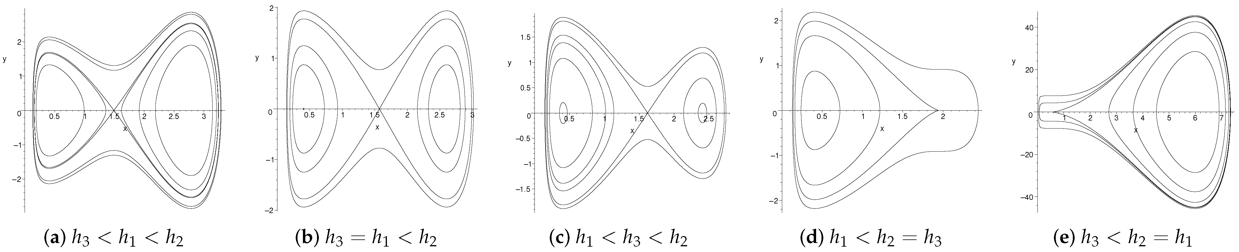
4. Explicit Exact Parametric Representations of the Solutions of the System (4) with Three Equilibrium Points and a₅ < 0

In this section, we use (13) to calculate the explicit exact parametric representations $\varphi \left(\xi \right)=\sqrt{\psi \left(\xi \right)}$ of solutions of the system (4) for the case that there exist three equilibrium points and $a_5<0$. The discussion is pretty similar as that in Section 3.

4.1. The Parametric Representations of the Bounded Orbits Given by Figure 2a

(i)

Corresponding to the level curves defined by $H_0(\varphi ,y)=h$ with $h\in (h_3,h_1)$, there exists a family of periodic orbits enclosing the equilibrium point $E_3({\varphi }_3,0)$ of the system (4). Now, (13) can be written as

$$\sqrt{{\displaystyle \frac{4|a_5|}{3}}}\xi ={\int }_{{\psi }_b}^{\psi }{\displaystyle \frac{d\psi }{\sqrt{({\psi }_a-\psi )({\psi }_b-\psi )[{(\psi -{\widehat{b}}_2)}^2+{\widehat{a}}_2^2]}}},$$

from which one has the parametric representation of the family of periodic solutions

$$\begin{array}{c}\hfill \psi \left(\xi \right)={\displaystyle \frac{({\psi }_a{B}_2+{\psi }_b{A}_2)-({\psi }_a{B}_2-{\psi }_b{A}_2)\mathrm{cn}({\Omega }_4\xi ,k))}{(A_2+B_2)+(A_2-B_2)\mathrm{cn}({\Omega }_4\xi ,k)}},\end{array}$$

(27)

where

$$\begin{array}{cc}\hfill A_2^2=& {({\psi }_a-{\widehat{b}}_2)}^2+{\widehat{a}}_2^2,B_2^2={({\psi }_b-{\widehat{b}}_2)}^2+{\widehat{a}}_2^2,\hfill \\ \hfill k^2=& {\displaystyle \frac{{({\psi }_a-{\psi }_b)}^2-{(A_2-B_2)}^2}{4A_2{B}_2}},{\Omega }_4=\sqrt{{\displaystyle \frac{4|a_5|A_2{B}_2}{3}}}.\hfill \end{array}$$

(ii)

Corresponding to the level curves defined by $H_0(\varphi ,y)=h$ with $h\in (h_1,h_2),$ there exist two families of periodic orbits of the system (4), enclosing the equilibrium point $E_1({\varphi }_1,0)$ and $E_3({\varphi }_3,0)$, respectively. For the left family of periodic orbits enclosing the center $E_1({\varphi }_1,0)$, (13) can be written as

$$\sqrt{{\displaystyle \frac{4|a_5|}{3}}}\xi ={\int }_{{\psi }_d}^{\psi }{\displaystyle \frac{d\psi }{\sqrt{({\psi }_a-\psi )({\psi }_b-\psi )({\psi }_c-\psi )(\psi -{\psi }_d)}}},$$

from which we obtain the parametric representation of this family of periodic solutions of the system (4) given by

$$\begin{array}{c}\hfill \psi \left(\xi \right)={\psi }_a-{\displaystyle \frac{{\psi }_a-{\psi }_d}{1-{\widehat{\alpha }}_3^2{\mathrm{sn}}^2({\Omega }_5\xi ,k)}},\end{array}$$

(28)

where

$${\widehat{\alpha }}_3^2={\displaystyle \frac{{\psi }_d-{\psi }_c}{{\psi }_a-{\psi }_c}},k^2={\displaystyle \frac{-{\widehat{\alpha }}_3^2({\psi }_a-{\psi }_b)}{{\psi }_b-{\psi }_d}}\mathrm{and}{\Omega }_5=\sqrt{{\displaystyle \frac{1}{3}}\left|a_5\right|({\psi }_a-{\psi }_c)({\psi }_b-{\psi }_d)}.$$

We notice that when h approaches $h_2$, the periodic orbit in the left family defined by $H_0(\varphi ,y)=h$ tends to the left homoclinic loop which is close to the singular straight line $\varphi =0$. Therefore, the left homoclinic orbit gives rise to an envelope pseudo-peakon solution, and the periodic orbit family gives rise to a pseudo-periodic peakon family (see Figure 6a,b).

Figure 6. The profiles of envelope wave given by the orbits in Figure 2a.

Similarly, for the right family of periodic orbits enclosing the center $E_3({\varphi }_3,0)$, (13) can be written as

$$\sqrt{{\displaystyle \frac{4|a_5|}{3}}}\xi ={\int }_{{\psi }_b}^{\psi }{\displaystyle \frac{d\psi }{\sqrt{({\psi }_a-\psi )(\psi -{\psi }_b)(\psi -{\psi }_c)(\psi -{\psi }_d)}}},$$

from which one has the parametric representation of this family of periodic solutions of the system (4) given by

$$\begin{array}{c}\hfill \psi \left(\xi \right)={\psi }_c+{\displaystyle \frac{{\psi }_b-{\psi }_c}{1-{\widehat{\alpha }}_4^2{\mathrm{sn}}^2({\Omega }_5\xi ,k)}},\end{array}$$

(29)

where

$${\widehat{\alpha }}_4^2={\displaystyle \frac{{\psi }_a-{\psi }_b}{{\psi }_a-{\psi }_c}},k^2={\displaystyle \frac{{\widehat{\alpha }}_4^2({\psi }_c-{\psi }_d)}{{\psi }_b-{\psi }_d}}\mathrm{and}{\Omega }_5=\sqrt{{\displaystyle \frac{1}{3}}\left|a_5\right|({\psi }_a-{\psi }_c)({\psi }_b-{\psi }_d)}.$$

(iii)

Corresponding to the level curves defined by $H_0(\varphi ,y)=h_2$, there exist two homoclinic orbits of the system (4) to the saddle point $E_2({\varphi }_2,0)$, enclosing the equilibrium point $E_1({\varphi }_1,0)$ and $E_3({\varphi }_3,0)$, respectively. For the right homoclinic orbit, (13) can be written as

$$\sqrt{{\displaystyle \frac{4|a_5|}{3}}}\xi ={\int }_{\psi }^{{\psi }_M}{\displaystyle \frac{d\psi }{(\psi -{\psi }_2)\sqrt{({\psi }_M-\psi )(\psi -{\psi }_m)}}},$$

from which the parametric representation of the bright envelope soliton solution of the system (4) is given by (see Figure 6d):

$$\begin{array}{c}\hfill \psi \left(\xi \right)={\psi }_2+{\displaystyle \frac{2({\psi }_M-{\psi }_2)({\psi }_2-{\psi }_m)}{({\psi }_M-{\psi }_m)cosh\left({\omega }_6\xi \right)-({\psi }_M+{\psi }_m-2{\psi }_2)}},\end{array}$$

(30)

where ${\omega }_6=\sqrt{{\displaystyle \frac{4}{3}}\left|a_5\right|({\psi }_M-{\psi }_2)({\psi }_2-{\psi }_m)}$.

For the left homoclinic orbit, (13) can be written as

$$\sqrt{{\displaystyle \frac{4|a_5|}{3}}}\xi ={\int }_{{\psi }_m}^{\psi }{\displaystyle \frac{d\psi }{({\psi }_2-\psi )\sqrt{({\psi }_M-\psi )(\psi -{\psi }_m)}}},$$

from which one has the following parametric representation of the dark envelope soliton solution of the system (4) given by

$$\begin{array}{c}\hfill \psi \left(\xi \right)={\psi }_2-{\displaystyle \frac{2({\psi }_M-{\psi }_2)({\psi }_2-{\psi }_m)}{({\psi }_M-{\psi }_m)cosh\left({\omega }_6\xi \right)+({\psi }_M+{\psi }_m-2{\psi }_2)}}.\end{array}$$

(31)

(iv)

Corresponding to the level curves defined by $H_0(\varphi ,y)=h$ with $h\in (h_2,\infty )$, there exists a global family of periodic orbits enclosing three equilibrium points $E_j({\varphi }_j,0),j=1,2,3$ of the system (4). In this case, this family has the same parametric representation as that of (27).

Note that there exists a segment of every periodic orbit in this periodic family for which it is very close to the singular straight line $\varphi =0$. This global periodic orbit family gives rise to a family of pseudo-periodic peakon solution of the system (4) (see Figure 6c).

Similarly, for the orbits shown in Figure 2b,c, one can calculate their parametric representations. We skip it here.

4.2. The Parametric Representations of the Homoclinic Orbit to the Cusp Point Given by Figure 2e

Corresponding to the level curves defined by $H_0(\varphi ,y)=h_1=h_2,$ there is a homoclinic orbit to the cusp point $E_1({\varphi }_1={\varphi }_2,0)$ enclosing the equilibrium point $E_3({\varphi }_3,0)$. Equation (13) can be written as

$$\sqrt{{\displaystyle \frac{4|a_5|}{3}}}\xi ={\int }_{\psi }^{{\psi }_M}{\displaystyle \frac{d\psi }{(\psi -{\psi }_1)\sqrt{({\psi }_M-\psi )(\psi -{\psi }_1)}}},$$

from which one has the parametric representation of the bright envelope soliton solution of the system (4) given by

$$\begin{array}{c}\hfill \psi \left(\xi \right)={\psi }_1+{\displaystyle \frac{{\psi }_M-{\psi }_1}{1+{\left({\omega }_7\xi \right)}^2}},\end{array}$$

(32)

where ${\omega }_7=({\psi }_M-{\psi }_1)\sqrt{{\displaystyle \frac{1}{3}}\left|a_5\right|}.$

For $\psi \left(\xi \right)$ given by (32), we have

$$\begin{array}{cc}\hfill \int {\displaystyle \frac{d\xi }{\psi \left(\xi \right)}}=& {\displaystyle \frac{1}{{\psi }_1}}\xi -{\displaystyle \frac{1}{{\psi }_1^2}}({\psi }_M-{\psi }_1)\int {\displaystyle \frac{{\psi }_{1}d\xi }{{\psi }_M+{\psi }_1{\left({\omega }_7\xi \right)}^2}}\hfill \\ \hfill =& {\displaystyle \frac{1}{{\psi }_1}}\xi -{\displaystyle \frac{{\psi }_M-{\psi }_1}{{\omega }_7{\psi }_1\sqrt{{\psi }_1{\psi }_M}}}{tan}^{-1}\left({\displaystyle \frac{\sqrt{{\psi }_1}{\omega }_7\xi }{\sqrt{{\psi }_M}}}\right).\hfill \end{array}$$

It follows that

$$\begin{array}{c}\hfill \theta \left(\xi \right)={\theta }_5\left(\xi \right)=\left({\displaystyle \frac{v+2\alpha \kappa }{2\alpha }}+{\displaystyle \frac{1}{{\psi }_1}}\right)\xi -{\displaystyle \frac{k_0({\psi }_M-{\psi }_1)}{\alpha {\omega }_7{\psi }_1\sqrt{{\psi }_1{\psi }_M}}}{tan}^{-1}\left({\displaystyle \frac{\sqrt{{\psi }_1}{\omega }_7\xi }{\sqrt{{\psi }_M}}}\right).\end{array}$$

(33)

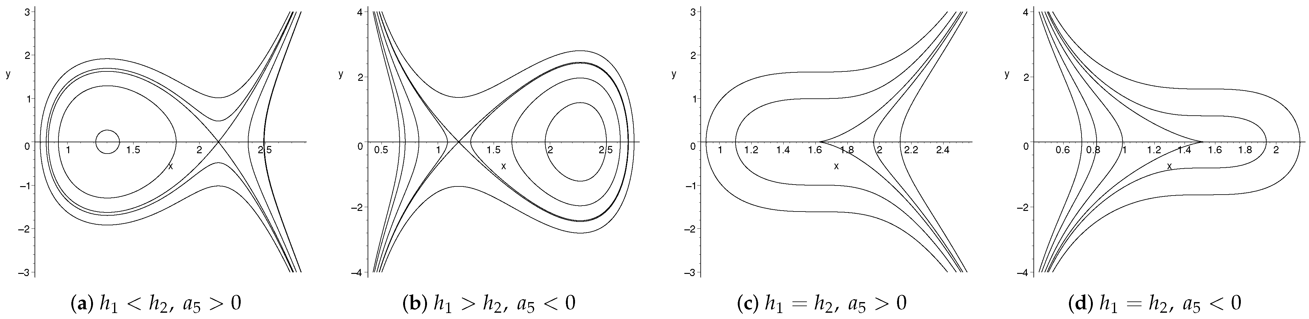
5. The Parametric Representations of the Homoclinic Orbit and Periodic Orbits Given by Figure 3b

Two cases will be discussed in this part.

(i)

Corresponding to the level curves defined by $H_0(\varphi ,y)=h$ with $h\in (h_2,h_1),$ there exist a family of periodic orbits enclosing the equilibrium point $E_2({\varphi }_2,0)$ of the system (4) and an open curve family which tends to the singular straight line $\varphi =0$ as $\left|y\right|\to \infty .$ For the periodic family, (13) can be written as

$$\sqrt{{\displaystyle \frac{4|a_5|}{3}}}\xi ={\int }_{{\psi }_b}^{\psi }{\displaystyle \frac{d\psi }{\sqrt{({\psi }_a-\psi )(\psi -{\psi }_b)(\psi -{\psi }_c)(\psi +{\psi }_d)}}},$$

from which one has the parametric representation of the family of periodic solutions of the system (4) given by

$$\begin{array}{c}\hfill \psi \left(\xi \right)={\psi }_c+{\displaystyle \frac{{\psi }_b-{\psi }_c}{1-{\widehat{\alpha }}_5^2\mathrm{s}{\mathrm{n}}^2({\Omega }_6\xi ,k)}},\end{array}$$

(34)

where

$${\widehat{\alpha }}_5^2={\displaystyle \frac{{\psi }_a-{\psi }_b}{{\psi }_a-{\psi }_c}},k^2={\displaystyle \frac{{\widehat{\alpha }}_5^2({\psi }_c+{\psi }_d)}{({\psi }_b+{\psi }_d)}}\mathrm{and}{\Omega }_6=\sqrt{{\displaystyle \frac{1}{3}}\left|a_5\right|({\psi }_a-{\psi }_c)({\psi }_b+{\psi }_d)}.$$

For the open curve family, (13) can be written as

$$\sqrt{{\displaystyle \frac{4|a_5|}{3}}}\xi ={\int }_{\psi }^{{\psi }_c}{\displaystyle \frac{d\psi }{\sqrt{({\psi }_a-\psi )({\psi }_b-\psi )({\psi }_c-\psi )(\psi +{\psi }_d)}}},$$

from which we obtain the parametric representation of the compacton solution family of the system (4) given by

$$\begin{array}{c}\hfill \psi \left(\xi \right)={\psi }_b-{\displaystyle \frac{{\psi }_b-{\psi }_c}{1-{\widehat{\alpha }}_6^2\mathrm{s}{\mathrm{n}}^2({\Omega }_6\xi ,k)}},\xi \in (-{\xi }_{04},{\xi }_{04}),\end{array}$$

(35)

where

$$\begin{array}{cc}\hfill {\widehat{\alpha }}_6^2=& {\displaystyle \frac{{\psi }_c+{\psi }_d}{{\psi }_b+{\psi }_d}},k^2={\displaystyle \frac{{\widehat{\alpha }}_6^2({\psi }_a-{\psi }_b)}{{\psi }_a-{\psi }_c}},\hfill \\ \hfill {\Omega }_6=& \sqrt{{\displaystyle \frac{1}{3}}\left|a_5\right|({\psi }_a-{\psi }_c)({\psi }_b+{\psi }_d)},{\xi }_{04}={\displaystyle \frac{1}{{\Omega }_6}}\mathrm{s}{\mathrm{n}}^{-1}\sqrt{{\displaystyle \frac{{\psi }_c}{{\widehat{\alpha }}_6^2{\psi }_b}}}.\hfill \end{array}$$

(ii)

Corresponding to the level curves defined by $H_0(\varphi ,y)=h_1,$ there exist a homoclinic orbit of the system (4) to the saddle point $E_1({\varphi }_1,0),$ enclosing the equilibrium point $E_2({\varphi }_2,0)$. Equation (13) can be written as

$$\sqrt{{\displaystyle \frac{4|a_5|}{3}}}\xi ={\int }_{\psi }^{{\psi }_M}{\displaystyle \frac{d\psi }{(\psi -{\psi }_1)\sqrt{({\psi }_M-\psi )(\psi +{\psi }_d)}}},$$

from which we have the the parametric representation of the bright envelope soliton solution of the system (4) given by

$$\begin{array}{c}\hfill \psi \left(\xi \right)={\psi }_1+{\displaystyle \frac{2({\psi }_M-{\psi }_1)({\psi }_1+{\psi }_d)}{({\psi }_M+{\psi }_d)cosh\left({\omega }_8\xi \right)-({\psi }_M-{\psi }_d-2{\psi }_1)}},\end{array}$$

(36)

where ${\omega }_8=\sqrt{{\displaystyle \frac{4}{3}}\left|a_5\right|({\psi }_M-{\psi }_1)({\psi }_1+{\psi }_d)}.$

6. Conclusions

In this work, we focus on the exact traveling wave solutions for the coupled nonlinear generalized Zakharov equations under the framework of the dynamical system approach [24,25]. As the first step, we obtain the bifurcations of the phase portraits associated with the planar Hamiltonian system (4), which is discussed in detail in Section 2. Based on it, all possible explicit parametric representations of bounded solutions are obtained, which include pseudo-periodic peakon, pseudo-peakon, smooth periodic wave solutions, solitary solutions, kink wave solution and the compacton solution family. The study in this work provides a better understanding of the model problem and corrects the mistake made in [1] as discussed in Section 1.

References

- Al Qahtani, S.A.; Alngar, M.E.M. Soliton Solutions for Coupled Nonlinear Generalized Zakharov Equations with Anti-cubic Nonlinearity Using Various Techniques. Int. J. Appl. Comput. Math. 2024, 10, 9. [Google Scholar] [CrossRef]
- Kudryashov, N.A. Optical solitons of the model with generalized anti-cubic nonlinearity. Optik 2022, 257, 168746. [Google Scholar] [CrossRef]
- Olver, P.J.; Rosenau, P. Tri-Hamiltonian duality between solitons and solitary-wave solutions having compact support. Phys. Rev. E 1996, 53, 1900–1906. [Google Scholar] [CrossRef] [PubMed]
- Camassa, R.; Holm, D.D. An integrable shallow water equation with peak solutions. Phys. Rev. Lett. 1993, 71, 1161–1164. [Google Scholar] [CrossRef]
- Camassa, R.; Holm, D.D.; Hyman, J.M. A new integrable shallow water equation. Adv. Appl. Mech. 1994, 31, 1–33. [Google Scholar]
- Camassa, R.; Hyman, J.M.; Luce, B.P. Nonlinear waves and solitons in physical systems. Phys. D 1998, 123, 1–20. [Google Scholar] [CrossRef]
- Degasperis, A.; Holm, D.D.; Hone, A.N.W. A new integrable equation with peakon solutions. Theoret. Math. Phys. 2002, 133, 1463–1474. [Google Scholar] [CrossRef]
- Degasperis, A.; Procesi, M. Asymptotic integrability. In Symmetry and Perturbation Theory; Degasperis, A., Gaeta, G., Eds.; World Scientific: Singapore, 1999; pp. 23–27. [Google Scholar]
- Fokas, A.S. On class of physically important integrable equations. Phys. D 1995, 87, 145–150. [Google Scholar] [CrossRef]
- Li, J.B.; Qiao, Z.J. Peakon, pseudo-peakon, and cuspon solutions for two generalized Camassa-Holm equations. J. Math. Phys. 2013, 54, 123501. [Google Scholar] [CrossRef]
- Li, J.B.; Zhou, W.J.; Chen, G.R. Understanding peakons, periodic peakons and compactons via a shallow water wave equation. Int. J. Bifur. Chaos 2016, 26, 1650207. [Google Scholar] [CrossRef]
- Novikov, V. Generalizations of the Camassa-Holm equation. J. Phys. A Math. Theor. 2009, 42, 342002. [Google Scholar] [CrossRef]
- Qiao, Z. A new integrable equation with cuspons and W/M-shape-peaks solitons. J. Math. Phys. 2006, 47, 112701–112710. [Google Scholar] [CrossRef]
- Li, J.B. Singular Nonlinear Traveling Wave Equations: Bifurcation and Exact Solutions; Science Press: Beijing, China, 2013. [Google Scholar]
- Li, J.B.; Chen, G.R. On a class of singular nonlinear traveling wave equations. Int. J. Bifurc. Chaos 2017, 17, 4049–4065. [Google Scholar] [CrossRef]
- Li, J.B.; Chen, G.R.; Song, J. Completing the study of traveling wave solutions for three two-component shallow water wave models. Internat. J. Bifur. Chaos 2020, 30, 2050036. [Google Scholar] [CrossRef]
- Li, J.B.; Han, M.A.; Ke, A. Bifurcations and exact traveling wave solutions of the Khorbatly’s geophysical Boussinesq system. J. Math. Anal. Appl. 2024, 537, 128263. [Google Scholar] [CrossRef]
- Li, J.B.; Liu, Z.R. Smooth and non-smooth traveling waves in a nonlinear dispersive equation. Appl. Math. Model 2000, 25, 41–56. [Google Scholar] [CrossRef]
- Li, J.B.; Liu, Z.R. Traveling wave solutions for a class of nonlinear dispersive equations. Chin. Ann. Math. 2002, 23, 397–418. [Google Scholar] [CrossRef]
- Liu, X.; Zhang, L.; Zhang, M. Studies on pull-in instability of all electrostatic MEMS actuator: Dynamical system approach. J. Appl. Anal. Comput. 2022, 12, 850–861. [Google Scholar]
- Zhang, L.; Han, M.; Zhang, M.; Khalique, C.M. A new type of solitary wave solution of the mKdV equation under singular perturbations. Int. J. Bifur. Chaos 2020, 30, 2050162. [Google Scholar] [CrossRef]
- Zhang, X.; Tian, Y.; Zhang, M.; Qi, Y. Mathematical studies on generalized Burgers Huxley equation and its singularly perturbed form: Existence of traveling wave solutions. Nonlinear Dyn. 2024, 3, 2625–2634. [Google Scholar] [CrossRef]
- Byrd, P.F.; Fridman, M.D. Handbook of Elliptic Integrals for Engineers and Scientists; Springer: Berlin/Heidelberg, Germany, 1971. [Google Scholar]
- Song, J. Bifurcations and exact traveling wave solutions of the (n+1) dimensional q-deformed double sinh-gordon equations. Discret. Cont. Dyn. Syst. S 2023, 16, 573–588. [Google Scholar] [CrossRef]
- Zhou, Y.; Zhuang, J.S.; Li, J.B. Bifurcations and exact traveling wave solutions in two nonlinear wave systems. Int. J. Bifur. Chaos 2021, 31, 2150093. [Google Scholar] [CrossRef]
Disclaimer/Publisher’s Note: The statements, opinions and data contained in all publications are solely those of the individual author(s) and contributor(s) and not of MDPI and/or the editor(s). MDPI and/or the editor(s) disclaim responsibility for any injury to people or property resulting from any ideas, methods, instructions or products referred to in the content. |
© 2025 by the authors. Licensee MDPI, Basel, Switzerland. This article is an open access article distributed under the terms and conditions of the Creative Commons Attribution (CC BY) license (https://creativecommons.org/licenses/by/4.0/).
Share and Cite
Song, J.; Li, F.; Zhang, M. Bifurcations and Exact Solutions of the Coupled Nonlinear Generalized Zakharov Equations with Anti-Cubic Nonlinearity: Dynamical System Approach. Mathematics 2025, 13, 217. https://doi.org/10.3390/math13020217
Song J, Li F, Zhang M. Bifurcations and Exact Solutions of the Coupled Nonlinear Generalized Zakharov Equations with Anti-Cubic Nonlinearity: Dynamical System Approach. Mathematics. 2025; 13(2):217. https://doi.org/10.3390/math13020217
Chicago/Turabian StyleSong, Jie, Feng Li, and Mingji Zhang. 2025. "Bifurcations and Exact Solutions of the Coupled Nonlinear Generalized Zakharov Equations with Anti-Cubic Nonlinearity: Dynamical System Approach" Mathematics 13, no. 2: 217. https://doi.org/10.3390/math13020217
APA StyleSong, J., Li, F., & Zhang, M. (2025). Bifurcations and Exact Solutions of the Coupled Nonlinear Generalized Zakharov Equations with Anti-Cubic Nonlinearity: Dynamical System Approach. Mathematics, 13(2), 217. https://doi.org/10.3390/math13020217