Article

Trajectory Tracking of WMR with Neural Adaptive Correction

1
Department of Computer and Network Engineering, College of Computer Science and Engineering, University of Jeddah, Jeddah 21959, Saudi Arabia
2
Instituto de Automatica, UNSJ-CONICET, San Juan CP 5400, Argentina
3
Department of Cybersecurity, College of Computer Science and Engineering, University of Jeddah, Jeddah 23218, Saudi Arabia
4
Department of Information Systems and Technology, College of Computer Science and Engineering, University of Jeddah, Jeddah 23218, Saudi Arabia
*
Author to whom correspondence should be addressed.
Mathematics 2025, 13(19), 3178; https://doi.org/10.3390/math13193178
Submission received: 31 August 2025 / Revised: 16 September 2025 / Accepted: 28 September 2025 / Published: 3 October 2025
(This article belongs to the Section C2: Dynamical Systems)

Abstract

Wheeled mobile robots (WMRs) are being increasingly integrated into various sectors such as logistics and transportation. However, their accurate trajectory tracking remains a challenge. To address this control issue, this study proposes a trajectory correction technique for a wheeled mobile robot (WMR). This proposal uses a functional-link neural network (FLNN) that adjusts the trajectory error with the aim of minimizing it. This error is propagated backward by adjusting the different parameters of the controller. The controller was designed using a combination of linearization feedback, sliding mode control, and FLNN, where the latter provides adaptability to the controller. Using the Lyapunov stability theory, the stability of the proposal was demonstrated. Experiments and simulation analyses were also carried out to demonstrate the practical feasibility of the proposal.

1. Introduction

1.1. Motivation

Wheeled mobile robots (WMRs) are autonomous vehicles with a wide range of applications, generally in areas such as transportation and logistics, hygiene, and defense. Particularly, WMRs are increasingly transforming logistics, transportation, and last-mile delivery by enhancing efficiency, reducing costs, and improving service flexibility. From autonomous scooters and delivery vans to self-driving vehicles, these systems enable rapid and reliable distribution of goods in urban and industrial environments. They optimize routing, adapt to dynamic traffic conditions, and reduce human labor dependence. As part of Logistics 4.0, they integrate with digital platforms to play a crucial role in building sustainable and intelligent transportation ecosystems [1]. However, their integration into the existing infrastructure may cause certain challenges to appear. Those challenges may vary from control and stability to communication issues, such as delays, mainly when they are remotely operated [2]. The literature proposes the control of autonomous wheeled vehicles designed as underactuated systems [3], obtaining excellent results in trajectory tracking. Trajectory control is a current field of research in the area of WMR control. However, these vehicles are affected by various disturbances and exogenous actions that impair their proper functioning. In the works of [4,5], a parameter projection technique is used to design the parameter estimator, and a form of state observer is proposed to facilitate the development of output feedback control. The derived adaptive backstepping control, which involves both input and output quantizations, ensures that all closed-loop signals are bounded, and the control performance in terms of the mean square error is adjustable by properly choosing certain design parameters. The effectiveness of the proposed scheme was validated by numerical simulation. Complementing this, disturbance-observer-based control (DOBC) in WMR integrates disturbance estimation to compensate for external perturbations, while data-driven methods bypass explicit model identification by relying on input–output data for controller synthesis. Recent data-driven DOBC frameworks for nonlinear networked systems achieve practical output regulation and input constraints satisfaction, enhancing adaptability in uncertain environments [6]. The advent of AI and the increase in onboard hardware processing power have led to the creation of new methods for controlling problems in WMR systems; among these, we can mention [7,8,9,10]. It is possible to use strategies based on sliding mode control (SMC), widely cited in the scientific literature, to improve stability and mitigate all possible uncertainties and disturbances affecting WMRs. In the study [11], a cascade controller for the dynamics and kinematics of non-holonomic mobile robots is presented. Similarly, the work of [12] uses adaptive control for dynamics. In both cases, they consider that disturbances and uncertainties act on the robot’s dynamics. The work of [13] proposes a sliding mode control (SMC) for trajectory tracking of an autonomous wheelchair modeled as a non-holonomic mobile robot (WMR). It focuses on ensuring accuracy and stability in the face of disturbances and non-holonomic constraints. The effectiveness of the controller is validated through simulations, improving autonomy and mobility. For their part, other authors [14] present an SMC-based technique to mitigate active noise, producing improvements in convergence speed and error reduction in tracking. In addition to SMC, nonlinear control together with adaptive control produce improvements in trajectories by effectively attenuating active uncertainties in WMR systems. For example, refs. [15,16] focused on control based on neuroadaptive techniques for unknown slippage, using neural networks that adjust their parameters in real time with the aim of minimizing tracking errors. Again, these uncertainties are considered to act only on the dynamics. Similarly, Shojaei et al. [17] designed an adaptive controller to minimize parametric uncertainties in non-holonomic WMRs using a combination of techniques based on nonlinear control. In the work by [18], the authors propose a double control loop based on SMC-Adaptable and Backstepping for WMR vehicles, taking into account the aspects of actuator failure and robot slippage, which includes an observer for actuator failures and another for disturbances. Improving the actions of the proposed control. In contrast, Scaglia et al. [19] and Petrov et al. [20] use a method based on linear algebra (LABC) and exponential trajectory tracking controller, respectively, for WMR vehicle control, obtaining responses with asymptotically stable error in both cases. Other alternative control techniques for WMR are proposed by [21] based on a switchable fractional order (FO) controller that can stabilize incommensurable states in finite time, where the control strategy reduces external disturbances. In this line of research, Ho et al. [22] present another proposal for controlling WMR vehicles. The authors use an adaptive integral terminal sliding mode control based on time delay estimation (AITSMC) as a dynamic controller to achieve tracking control and eliminate the effects of disturbances and uncertainties. This control strategy ensures that tracking errors remain bounded.
Based on the analysis of the previous literature, the main objective of this article is to apply an advanced adaptive control method that unifies the variations and uncertainties of the model (kinematics and dynamics) to reduce trajectory tracking error. The proposed solution employs a control structure based on feedback linearization using sliding surfaces with neuroadaptive capability, based on functional-link neural networks (FLNNs). This integrated approach not only allows the system to respond quickly to disturbances, but also self-adjusts internal parameters to reduce trajectory error. The result is greater robustness, adaptability, and stability for WMR vehicles, which significantly improves performance in real operating conditions.

1.2. Contributions

The main points of interest of the proposed method are as follows:
  • This proposal presents a design for FLNN-based controllers, which do not require complete knowledge of the system dynamics. Some studies have shown the weakness of regression-based adaptive control in structures [23]. Where the adaptive controller was ineffective if any element of the regression vector was unknown (especially if it corresponded to model uncertainties), this technique, developed based on feedback linearization, SMC, and FLNN, is a solid proposal.
  • This paper provides a rigorous analysis of the trajectory tracking control of WMR system, focusing on the control parameter conditions necessary to assure convergence spite the dynamic uncertainties. By examining the interaction dynamics between WMR and its surroundings, this study explores the effectiveness of adaptive neural network control considering the whole dynamics.
  • The theory presented in this paper is validated by numerical simulations. For the simulation, a five-degree-of-freedom kinematics and dynamics model was selected to represent the WMR. This simulation demonstrates the effectiveness of the control scheme in managing disturbances and kinematics and dynamics uncertainties. The main objective of this article is to apply an advanced adaptive control method that unifies the variations and uncertainties of the model (kinematics and dynamics) in a global structure to reduce trajectory tracking error. The proposed solution employs a control structure based on feedback linearization using sliding surfaces with neuroadaptive capability, based on functional-link neural networks (FLNNs). This integrated approach not only allows the system to respond quickly to incertainties, but also self-adjusts internal neural parameters to reduce trajectory error. The result is greater robustness, adaptability, and stability for WMR vehicles, which significantly improves performance in real operating conditions.
  • This work presents comprehensive simulations and theoretical analyses, ensuring system stability using the Lyapunov stability theory.

1.3. Organization

The content of this document is organized as follows. Section 2 presents the mathematical model of the WMR. Section 3 addresses the description of the problem, presenting the uncertainties and external disturbances that affect the system. Section 4 presents the SMC technique that will be applied to the design of the base controller, and the neural structures for global dynamics adjustment are shown in the following section (Section 5). Section 6 presents the stability analysis of the proposed technique along with the rules for adjusting the parameters of the neural network. The simulation results are shown in Section 7. Finally, Section 8 concludes the document.

2. WMR Model

This section presents the mathematical model of the WMR (based on a unicycle), as shown in Figure 1, which indicates the parameters and variables of interest for controlling the vehicle. The mathematical representation of the complete model is described in [12,24] and shown below.
Kinematic model
r ˙ x ( t ) r ˙ y ( t ) Ψ ˙ ( t ) = v ( t ) cos Ψ ( t ) ω ( t ) a sin Ψ ( t ) v ( t ) sin Ψ ( t ) + ω ( t ) a cos Ψ ( t ) ω ( t ) + δ r 1 δ r 2 0
Dynamic model
v ˙ ( t ) ω ˙ ( t ) = ϑ 3 ϑ 1 ω 2 ( t ) ϑ 4 ϑ 1 v ( t ) ϑ 5 ϑ 2 ω ( t ) v ( t ) ϑ 6 ϑ 2 ω ( t ) + 1 ϑ 1 0 0 1 ϑ 2 u v ( t ) u ω ( t ) + δ v δ ω
where:
  • r x , r y are the coordinates of WMR in the XY plane.
  • r r e f x , r r e f y are the desrired coordinates of WMR in the XY plane.
  • v and ω are the linear and angular velocities developed by the WMR, respectively.
  • G indicates the robot’s center of mass.
  • c is the position of the rotating wheel.
  • E is the location of the tool it carries (e.g., lidar or sensors, depending on the application).
  • h is the point where the vehicle is referenced containing the coordinates r x , r y .
  • Ψ indicates the orientation of the robot.
  • a is the difference between the reference point and the center point of the virtual axis connecting the drive wheels.
The parameters of the dynamic model are indicated in the Table 1. These parameters depend on the diameter of the wheels, vehicle mass, inertia, center of mass, friction, motor and servo parameters, etc., and are described in Appendix B.
The uncertainty parameters acting on the WMR are indicated as δ r 1 , δ r 2 , δ v , and δ ω . δ r 1 and δ r 2 are functions that depend on the robot’s speeds and orientation, but there are uncertainties introduced by the sensors. On the other hand, δ v and δ ω depend on the parameters of the WMR (e.g., mass, inertia, wheel dimensions and tire deformation, parameters of the control servos and traction motors, etc.). These are considered perturbations. The WMR vehicle is initially analyzed with a kinematic part and a dynamic part, as indicated in (1) and (2), respectively, and shown in Figure 1.
Finally, using the feedback linearization technique, the unified model of the mobile robot will be obtained, on which the proposed controller will be designed.

3. Model Reformulation

The dynamic and kinematic model of the WMR must be reformulated to obtain a linear affine model, which is described by the following equations:
x ˙ 1 = x 4 cos ( x 3 ) x 5 a sin ( x 3 ) + δ r 1 x ˙ 2 = x 4 sin ( x 3 ) + x 5 a cos ( x 3 ) + δ r 2 x ˙ 3 = x 5 , x ˙ 4 = ϑ 3 ϑ 1 x 5 2 ϑ 4 ϑ 1 x 4 + 1 ϑ 1 u 1 + δ v , x ˙ 5 = ϑ 5 ϑ 2 x 5 x 4 ϑ 6 ϑ 2 x 5 + 1 ϑ 2 u 2 + δ ω ,
where
  • x = ( x 1 , x 2 , x 3 , x 4 , x 5 ) T = [ x , y , θ , v , ω ] T is the state vector.
  • u = ( u 1 , u 2 ) T = [ u ω , u v ] T are the control inputs (control actions for ω and v).
  • ϑ i is i = 1 t o 6 , WMR parameters.
  • δ i is i = r 1 , r 2 , v , ω , disturbances and unmodeled dynamics.
  • Outputs: y = ( y 1 , y 2 ) T = ( x 1 , x 2 ) T = ( r x , r y ) T .
The standard system without disturbance can be written as
x ˙ = f ( x ) + g u ,
The perturbed system is written as
x ˙ = f ( x ) + f ˜ ( x ) + g u ,
where
f ( x ) = x 4 cos ( x 3 ) x 5 a sin ( x 3 ) x 4 sin ( x 3 ) + x 5 a cos ( x 3 ) x 5 ϑ 3 ϑ 1 x 5 2 ϑ 4 ϑ 1 x 4 ϑ 5 ϑ 2 x 5 x 4 ϑ 6 ϑ 2 x 5 , g = 0 0 0 0 0 0 1 ϑ 1 0 0 c 1 ϑ 2 , u = u 1 u 2 , f ˜ ( x ) = δ r 1 δ r 2 0 δ v δ ω .
The output function is
h ( x ) = h 1 ( x ) h 2 ( x ) = x 1 x 2 .
Assumption 1. 
The uncertain f ˜ ( x ) is bounded by a constant f ˜ ( x ) δ f .

4. SMC Controller Design

For this initial analysis, we consider the multivariable system of the WMR robot indicated in (4), which will later be expanded to the complete system considering additive variations (5). Taking into account the theory of linearization by feedback [25], and applying it to model (4), the exact input–output linearization is performed, where the number of inputs is equal to the number of outputs. Differentiating r i with respect to time, the following equation is obtained:
d 2 d t 2 y 1 ( t ) y 2 ( t ) = L f 2 h 1 ( x ) L f 2 h 2 ( x ) + L g 1 h 1 ( x ) L g 2 h 1 ( x ) L g 1 h 2 ( x ) L g 2 h 2 ( x ) u 1 u 2
where L f 2 h i ( x ) is the i-th Lie derivative belonging to the function h ( x ) considering the vector field f ( x ) . Since the relative degree of all outputs is two, then for each output r i the terms L g , j h i ( x ) must be nonzero and the input u j will appear in the second derivative of the output y.
the Lie derivatives of each element of (8) (see Appendix A) are
L f 2 h 1 ( x ) = x 5 x 4 sin ( x 3 ) + x 5 a cos ( x 3 ) + + ϑ 3 ϑ 1 x 5 2 ( t ) ϑ 4 ϑ 1 x 4 cos ( x 3 ) ϑ 5 ϑ 2 x 5 x 4 ϑ 6 ϑ 2 x 5 a sin ( x 3 ) L f 2 h 2 ( x ) = x 5 x 4 sin ( x 3 ) + x 5 a cos ( x 3 ) + + ϑ 3 ϑ 1 x 5 2 ϑ 4 ϑ 1 x 4 sin ( x 3 ) + ϑ 5 ϑ 2 x 5 x 3 ϑ 6 ϑ 2 x 5 a cos ( x 3 )
and
L g 1 h 1 ( x ) = 1 ϑ 1 cos ( x 3 ) L g 1 h 2 ( x ) = 1 ϑ 2 a sin ( x 3 ) L g 2 h 1 ( x ) = 1 ϑ 1 sin ( x 3 ) L g 2 h 2 ( x ) = 1 ϑ 2 a cos ( x 3 )
Defining the output tracking error as
e = y y r e f = r 1 r 1 r e f r 2 r 2 r e f
The solution to this control proposal is to apply the feedback linearization method, which can self-adjust based on the error defined in (9). One possible configuration is to use a neural network whose inputs contain information about the system to be controlled and can adjust the controller parameters to reduce the tracking error. The implication of using a neural network is the introduction of an intrinsic approximation error ϵ [26], which is why it is important to combine adaptability with sliding surface techniques (SMC) to reduce the side effects of neural approximation [11]. Basically, this proposal defines a control law such that the state of the closed-loop system follows the desired state y i , with the possibility that the tracking error e converges to zero. Based on the above, we define a sliding surface σ ( t ) for a MIMO system of the form
σ ( t ) = d d t + γ 1 0 0 d d t + γ 2 e ( t ) = e 1 ( t ) + γ x e 1 ( t ) e 2 ( t ) + γ 2 e 2 ( t )
Now, deriving the sliding surface, we obtain
d σ ( t ) d t = d d t d d t e 1 ( t ) + γ 1 e 1 ( t ) d d t e 2 ( t ) + γ 2 e 2 ( t ) = d 2 e 1 ( t ) d t 2 + γ 1 d d t e 1 ( t ) d 2 e 2 ( t ) d t 2 + γ 2 d d t e 2 ( t )
Considering the definition of error (9), the above equation can be rewritten as
d σ ( t ) d t = d d t σ 1 ( t ) σ 2 ( t ) = d 2 r 1 ( t ) r 1 r e f ( t ) d t 2 + γ 1 d d t e 1 ( t ) d 2 r 2 ( t ) r 2 r e f ( t ) d t 2 + γ 2 d d t e 2 ( t )
In order to make the system state tracks remain on the sliding surface, let d σ i ( t ) d t = 0 , then
d σ ( t ) d t = d d t σ 1 ( t ) σ 2 ( t ) = = L f 2 h 1 ( x ) + L g 1 h 1 ( x ) u 1 + L g 2 h 1 ( x ) u 2 d 2 r 1 r e f ( t ) d t 2 + γ 1 d d t e 1 ( t ) L f 2 h 2 ( x ) + L g 1 h 2 ( x ) u 1 + L g 2 h 2 ( x ) u 2 d 2 r 2 r e f ( t ) d t 2 + γ 2 d d t e 2 ( t ) = 0 0
Now, based on (13), a control law can be proposed adding a discontinuous term u σ . This control law is presented in the form
u 1 u 2 = L g 1 h 1 ( x ) L g 2 h 1 ( x ) L g 1 h 2 ( x ) L g 2 h 2 ( x ) 1 κ 1 σ 1 L f 2 h 1 ( x ) + d 2 d t 2 r 1 r e f ( t ) γ 1 d d t e 1 ( t ) u σ 1 κ 2 σ 2 L f 2 h 2 ( x ) + d 2 d t 2 r 2 r e f ( t ) γ 2 d d t e 2 ( t ) u σ 2
Definition 1. 
Being u σ i ( t ) = κ σ i s i g n ( σ i ( t ) ) defined by (see [27] ), this term guarantees the sliding condition; the function sign(.) is defined by
if σ i > 0 t h e n s i g n ( σ i ) = 1 if σ i = 0 t h e n s i g n ( σ i ) = 0 if σ i < 0 t h e n s i g n ( σ i ) = 1
Lemma 1 
(Barbalat’s lemma [25]). Let ϕ : R R be a uniformly continuous function on [ 0 , ) . Suppose that lim t 0 t ϕ ( τ ) d τ exists and is finite. Then,
ϕ ( t ) 0 as t .
Now, we analyze the stability of the control proposal using Lyapunov’s criterion, for which we must define a positive definite quadratic. In this case, it is of the form
L ( σ ) = 1 2 σ T σ
Deriving the above Equation (16) with respect to time, and replacing (12) and (8) leads to
d d t L ( σ ) = σ T d ( σ ) d t = σ T d 2 r ( t ) r r e f ( t ) d t 2 + γ 1 0 0 γ 2 d d t e ( t ) =   = σ T ( L f 2 h 1 ( x ) L f 2 h 2 ( x ) + L g 1 h 1 ( x ) L g 2 h 1 ( x ) L g 1 h 2 ( x ) L g 2 h 2 ( x ) u 1 u 2 d 2 r r e f ( t ) d t 2 + γ 1 0 0 γ 2 d d t e ( t ) )
Replacing the control law proposed in (14), we obtain
d d t L ( σ ) = σ T d ( σ ) d t = σ T κ 1 0 0 κ 2 σ κ σ 1 0 0 κ σ 2 s i g n ( σ ) λ m i n κ 1 0 0 κ 2 σ 2 λ m i n κ σ 1 0 0 κ σ 2 σ < 0
It can be observed that in Equation (18), the first derivative of Lyapunov is less than or equal to zero, resulting in an asymptotically stable system. This proposal does not take into account the undesirable dynamic variations f ˜ ( x ) . Sliding mode control (SMC) is generally used to improve the robustness of the closed loop when the system is subject to limited external disturbances and uncertainties caused by unmodeled dynamics. However, increasing the κ σ i gain of the discontinuous term produces the chattering effect. This effect can cause damage or alterations in electromechanical systems. A possible solution to avoid increasing the gain is to use an adaptive control based on neural networks [11] in combination. This adaptive term should compensate for the uncertainties and disturbances in the system. In the following section, these variations will be characterized and a complete control technique will be proposed.

Uncertainties and Dynamic Variations

The main objective of this proposal is to reduce the tracking error caused by external disturbances or possible dynamic variations ( f ˜ ( x ) ). Therefore, a control proposal must be designed to ensure that the system variables are bounded for a closed-loop system when tracking a vector of desired signals y r e f . To obtain a control law over the perturbed system (5), we must analyze again considering the dynamic variations f ˜ ( x ) , so we can calculate the Lie derivatives as follows:
L ( f + f ˜ ) ( h i ( x ) ) = h i ( x ) x f i + f ˜ i = h i ( x ) x f i + h i ( x ) x f ˜ i Δ i
with Δ i being a term that denotes undesiderable variations on the dynamics. Taking into account (19), the new expression of WMR dynamics is
d d t r 1 ( t ) r 2 ( t ) = L f 2 h 1 ( x ) + Δ 1 L f 2 h 2 ( x ) + Δ 2 + L g 1 h 1 ( x ) L g 2 h 1 ( x ) L g 1 h 2 ( x ) L g 2 h 2 ( x ) u 1 u 2 = = L f 2 h 1 ( x ) L f 2 h 2 ( x ) + L g 1 h 1 ( x ) L g 2 h 1 ( x ) L g 1 h 2 ( x ) L g 2 h 2 ( x ) u 1 u 2 + Δ 1 Δ 2
where
Δ = Δ 1 Δ 2
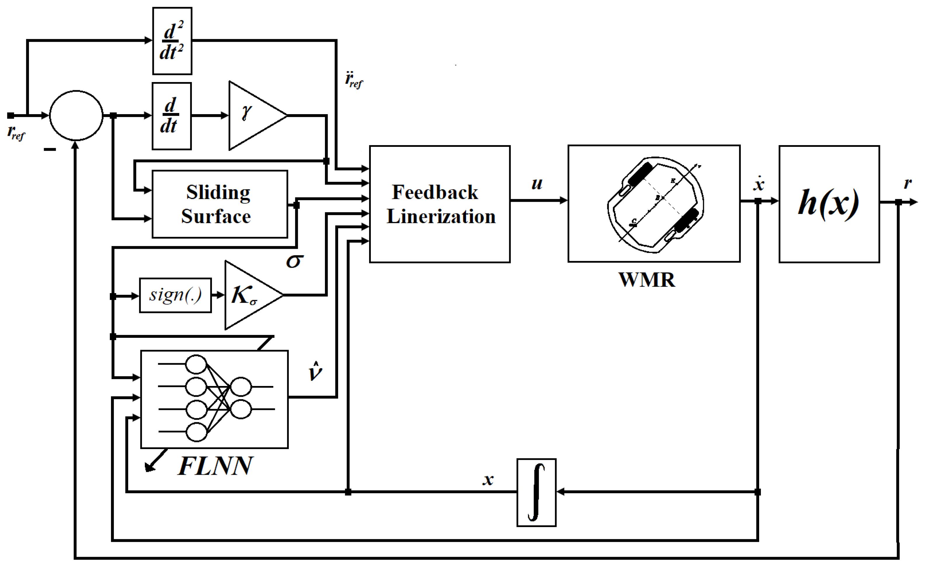
Equation (20) is the complete representation of the WMR, which includes variations not only in vehicle dynamics but also external disturbances that can affect kinematics. The control law proposed for this model (Figure 2) is indicated in
u 1 u 2 = L g 1 h 1 ( x ) L g 2 h 1 ( x ) L g 1 h 2 ( x ) L g 2 h 2 ( x ) 1 κ 1 σ 1 L f 2 h 1 ( x ) + d 2 d t 2 r 1 r e f ( t ) γ 1 d d t e 1 ( t ) υ ^ 1 u σ 1 κ 2 σ 2 L f 2 h 2 ( x ) + d 2 d t 2 r 2 r e f ( t ) γ 2 d d t e 2 ( t ) υ ^ 2 u σ 2
The structure of the neural network NN is shown in the following section.

5. Adaptive Neural Network Implementation

In this section, a neural network defined as a functional-link neural network (FLNN) is implemented. The function Δ R 2 × 1 must be approximated, being a smooth function and also since x is restricted to a compact set S of R n . Then, the uncertainty function Δ ( x ) can be approximated using the FLNN network [28]:
Δ = w T φ ( W T x ¯ ) + ϵ
or expressing the neural network in terms of the elements of the uncertainty function ( Δ )
Δ 1 Δ 2 = w 1 T w 2 T φ ( W T x ¯ ) + ϵ 1 ϵ 2
where w R m × 2 is the ideal output weight matrix, φ R m is the activation function consisting of the hyperbolic tangent function, W R d i m ( x ¯ ) × m is the input weight matrix, x ¯ = [ x , x ˙ , σ ] R b is the input signal vector, and ϵ R 2 × 1 is the approximation error. Moreover, b is the number of input signals and m is the number of neurons in the hidden layer.
Assumption 2. 
The ideal weights of the neural network, denoted as w (output weights) and W (hidden weights), are bounded, such that w i w i M and W W i M , where w i M and W i M are positive constant.
Assumption 3. 
The approximation error of the neural network is bounded by a known positive constant ε i M , such that ϵ ¯ i ( x i ) ε i M for all x i D , where D represents the input domain, and where the neural network-based estimator is defined as
υ ^ ( x ) = υ ^ 1 υ ^ 2 = w ^ T φ ( W ^ T x ¯ ) = w ^ 1 T w ^ 2 T φ ( W ^ T x ¯ ) ,
To obtain the differential equation of the d d t σ , we replace the WMR model (20) in (12), and we obtain
d σ ( t ) d t = d d t σ 1 ( t ) σ 2 ( t ) = L f 2 h x ( x ) L f 2 h y ( x ) + L g 1 h 1 ( x ) L g 2 h 1 ( x ) L g 1 h 2 ( x ) L g 2 h 2 ( x ) u 1 u 2 + + Δ 1 Δ 2 d 2 r 1 r e f ( t ) d t 2 d 2 r 2 r e f ( t ) d t 2 + κ 1 d d t e 1 ( t ) κ 2 d d t e 2 ( t )
Now, it is necessary to close the control loop, which will be used to determine the stability of the proposed control system, replacing the control law (21) in (25)
d d t σ 1 ( t ) σ 2 ( t ) = κ 1 0 0 κ 2 σ 1 σ 2 υ ^ 1 υ ^ 2 u σ 1 u σ 2 + Δ 1 Δ 2
Expressing (26) in scalar form, we obtain
d d t σ i ( t ) = κ i σ i υ ^ i u σ i + Δ i f o r i = 1 , 2
In the above Equation (27), the last term represents the dynamic variations of the model produced by uncertainties or external disturbances. These variations affect normal trajectory tracking.

6. Stability Analysis and Tuning Laws

We must now demonstrate that the proposed control law (21) can make the system immune to unwanted uncertainties.
Defining the Lyapunov candidate as
L ( σ , w ˜ , W ˜ ) = 1 2 1 2 σ i 2 + t r ( w ˜ i T Γ 1 w ˜ i ) + 1 2 t r ( W ˜ T H 1 W ˜ )
Deriving (28)
d d t L ( σ , w ˜ , W ˜ ) = 1 2 σ i d d t σ i + t r ( w ˜ i T Γ 1 d d t w ˜ i ) + t r ( W ˜ T H 1 d d t W ˜ )
Replacing (27) leads to
d d t L ( σ , w ˜ , W ˜ ) = 1 2 σ i T κ i σ i υ ^ i u σ i + Δ i + t r ( w ˜ i T Γ 1 d d t w ˜ i ) + + t r ( W ˜ T H 1 d d t W ˜ )
Replacing the neural estimator (24) and the approximate value of the uncertainties (23) in Equation (30), we obtain the following expression:
d d t L ( σ , w ˜ , W ˜ ) = 1 2 [ σ i κ i σ i w ^ i T φ ( W ^ T x ¯ ) u σ i + w i T φ ( W T x ¯ ) + ϵ i + + t r ( w ˜ i T Γ 1 d d t w ˜ i ) ] + t r ( W ˜ T H 1 d d t W ˜ )
The output weight error and the hidden weight error of the neural network, denoted w ˜ and W ˜ , respectively, are defined as the difference between the optimal output weight vector w and the estimate output weight vector w ^ of the neural network and, in the same form for the hidden weight ( W and W ˜ ), are defined as
w ˜ = w w ^ W ˜ = W W ^
For simplicity, we define the annotation of L ( σ , w ˜ , W ˜ ) as L and the activation functions φ ( W T x ¯ ) = φ and φ ( W ^ T x ¯ ) = φ ^ and defining the hidden-layer output error for a given x ¯ as φ ( W T x ¯ ) φ ( W ^ T x ¯ ) = φ φ ^ = φ ˜ .
Taking into account (31) and adding and subtracting the term w i T φ ^ leads to
d d t L = 1 2 [ σ i ( κ i σ i + w ^ i T φ ^ + w i T φ + w i T φ ^ w i T φ ^   u σ i + ϵ i ) + t r ( w ˜ i T Γ 1 d d t w ˜ i ) ] ( W ˜ T H 1 d d t W ˜ ) =   = 1 2 [ σ i κ i σ i + w ˜ i T φ ^ + w i T φ ˜ u σ i + ϵ i + + t r ( w ˜ i T Γ 1 d d t w ˜ i ) ] + t r ( W ˜ T H 1 d d t W ˜ )
Again, adding and subtracting w ^ i T φ ˜ , we obtain a new expression for d d t L , which is
d d t L = 1 2 [ σ i ( κ i σ i + w ˜ i T φ ^ + w i T φ ˜ + w ^ i T φ ˜ w ^ i T φ ˜   u σ i + ϵ i ) + t r ( w ˜ i T Γ 1 d d t w ˜ i ) ] + t r ( W ˜ T H 1 d d t W ˜ ) =   = 1 2 [ σ i ( κ i σ i + w ˜ i T φ ^ + w ˜ i T φ ˜ + w ^ i T φ ˜ u σ i + ϵ i ) + t r ( w ˜ i T Γ 1 d d t w ˜ i ) ] + t r ( W ˜ T H 1 d d t W ˜ )
If we consider a Taylor series approximation for φ ˜ , we obtain
φ ˜ = d d t φ ( W ^ T x ¯ ) W ˜ T x ¯ + O ( W ˜ T x ¯ ) 2 = d d t φ ^ W ˜ T x ¯ + O ( W ˜ T x ¯ ) 2 = = d d t φ ˜ ( W T W ^ T ) x ¯ + O ( W ^ T x ¯ ) 2
Denoting d d t φ ( W ^ T x ¯ ) = d d t φ ˜ .
Replacing (34) with (35) leaves us with
d d t L = 1 2 [ σ i ( κ i σ i + w ˜ i T φ ^ w ˜ i T d d t φ ^ W ^ T x ¯ + w ^ i T d d t φ ^ W ˜ T x ¯ u σ i + ϵ i ) + t r ( w ˜ i T Γ 1 d d t w ˜ i ) ] + t r ( W ˜ T H 1 d d t W ˜ )
defining ϵ ¯ i = w ˜ i T d d t φ ^ W T x ¯ + O i ( W ˜ T x ¯ ) 2 + ϵ i .
The following adaptation laws of the neural weights, denoted by w ^ and W ^ , of the neural networks are proposed as
d d t w ^ i = Γ φ ^ σ i T Γ d d t φ ^ W ^ T x ¯ σ i T η Γ σ w ^ i d d t W ^ = H x ¯ ( d d t φ ^ T w ^ i σ i ) T η H σ W ^
where η is a positive constant. In practice, η are positive very small values because the main function of the second terms of (37) is to avoid some drift if the input vector to the neural networks are not persistently exciting [26]. Now, considering that t r ( a ) = a , where a is a scalar, and using the cyclic property of trace, Equation (36) can be rewritten as
d d t L = 1 2 [ σ i ( κ i σ i + w ˜ i T φ ^ w ˜ i T d d t φ ^ W ^ T x ¯ + w ^ i T d d t φ ^ W ˜ T x ¯ u σ i + ϵ i ) + t r ( w ˜ i T Γ 1 d d t w ˜ i ) ] + t r ( W ˜ T H 1 d d t W ˜ )
Replacing the adjustment law indicated by the equations in (37) in (39), we obtain
d d t L = 1 2 [ κ i σ i 2 + σ i w ˜ i T φ ^ w ˜ i T d d t φ ^ W ^ T x ¯ + σ i w ^ i T d d t φ ^ W ˜ T x ¯   σ i u σ i + σ i ϵ i + t r w ˜ i T ( φ ^ σ i T + d d t φ ^ W ^ T x ¯ σ i T + η σ w ^ i ) ] + + t r ( W ˜ T x ¯ ( d d t φ ^ T w ^ i σ i ) T + η σ W ^ )
Taking into account that t r W ˜ T x ¯ ( d d t φ ^ T w ^ i σ i ) T = σ i w ^ i T d d t φ ^ W ˜ T x ¯ and t r ( W ˜ T x ¯ ( d d t φ ^ T w ^ i σ i ) T ) = σ i w ^ i T d d t φ ^ W ˜ T x ¯
d d t L = 1 2 κ i σ i 2 σ i u σ i + σ i ϵ i + t r ( η σ w ˜ i T w ^ i ) + t r η σ W ˜ T W ^
Using Definition 1, remembering that 1 2 | σ i | = σ 1 , and considering the difference (32) leads to
d d t L = 1 2 κ i σ i 2 κ σ i | σ i | + σ i ϵ ¯ i + t r ( η σ ( σ w ˜ i T ( w i w ˜ i ) ) + t r η σ W ˜ T ( W W ˜ )
No, by adding and subtracting w i M 2 4 in (40), and rearranging, we obtain
d d t L = 1 2 κ i σ i 2 κ σ i | σ i | + σ i ϵ ¯ i η σ w ˜ i w i M 2 ) 2 + η σ w i M 2 4   η σ W ˜ W i M 2 ) 2 + η σ W i M 2 4   λ m i n ( κ ) σ 2 2 η σ 1 2 w ˜ i w i M 2 ) 2 η σ W ˜ W i M 2 ) 2 σ 1 λ m i n ( κ σ ) ε i M η σ 1 2 w i M 2 4 η σ W i M 2 4
Note with a sufficiently large value for δ m and κ σ such that λ m i n { κ σ } > η W i M 2 4 + η x y w i M 2 4 + ε i M , it is satisfied that d d t L 0 , indicating that d d t L is a semi-definite negative. In practice, η are positive very small values because the main function of the second terms of (37) is to avoid some drift if the input vector to the neural networks are not persistently exciting.
Futhermore, according to Lemma 1, lim t σ ( t ) = 0 . This further implies that lim t d e ( t ) d t = 0 . Therefore, from (10), it is also true that
lim t e ( t ) = 0 ,

7. Simulation

7.1. Results

This section presents some of the results to show the performance of the proposed control technique. Several simulations were carried out, including active disturbances on the WMR. Our institute has Pioneer 2DX and 3DX mobile robots, which accept linear and angular velocities as input reference signals. The original Pioneer 2DX has an 800 MHz Pentium III with odometric sensors, whose sensitivity is 1 mm for position, 1 mm/s for linear velocity, and 1°/s for angular velocity. These are currently undergoing a hardware upgrade (Rasberry Pi). The configuration parameters of the experiment are κ 1 = κ 2 = 2 , x = 0.0, and y = 0.00. The FLNN configuration has m = 5 (neurons) with two outputs, and the weights w and W were set randomly.
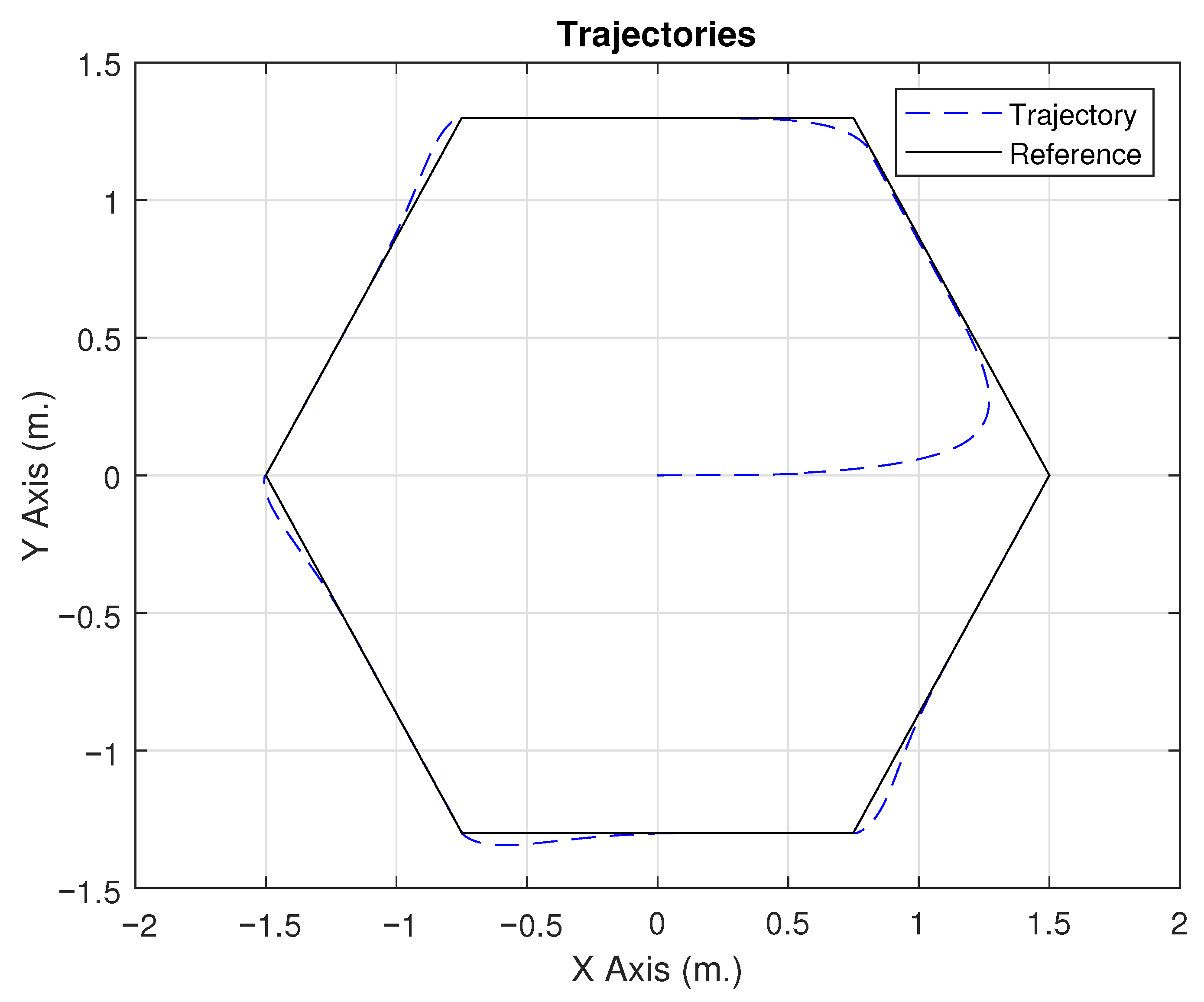
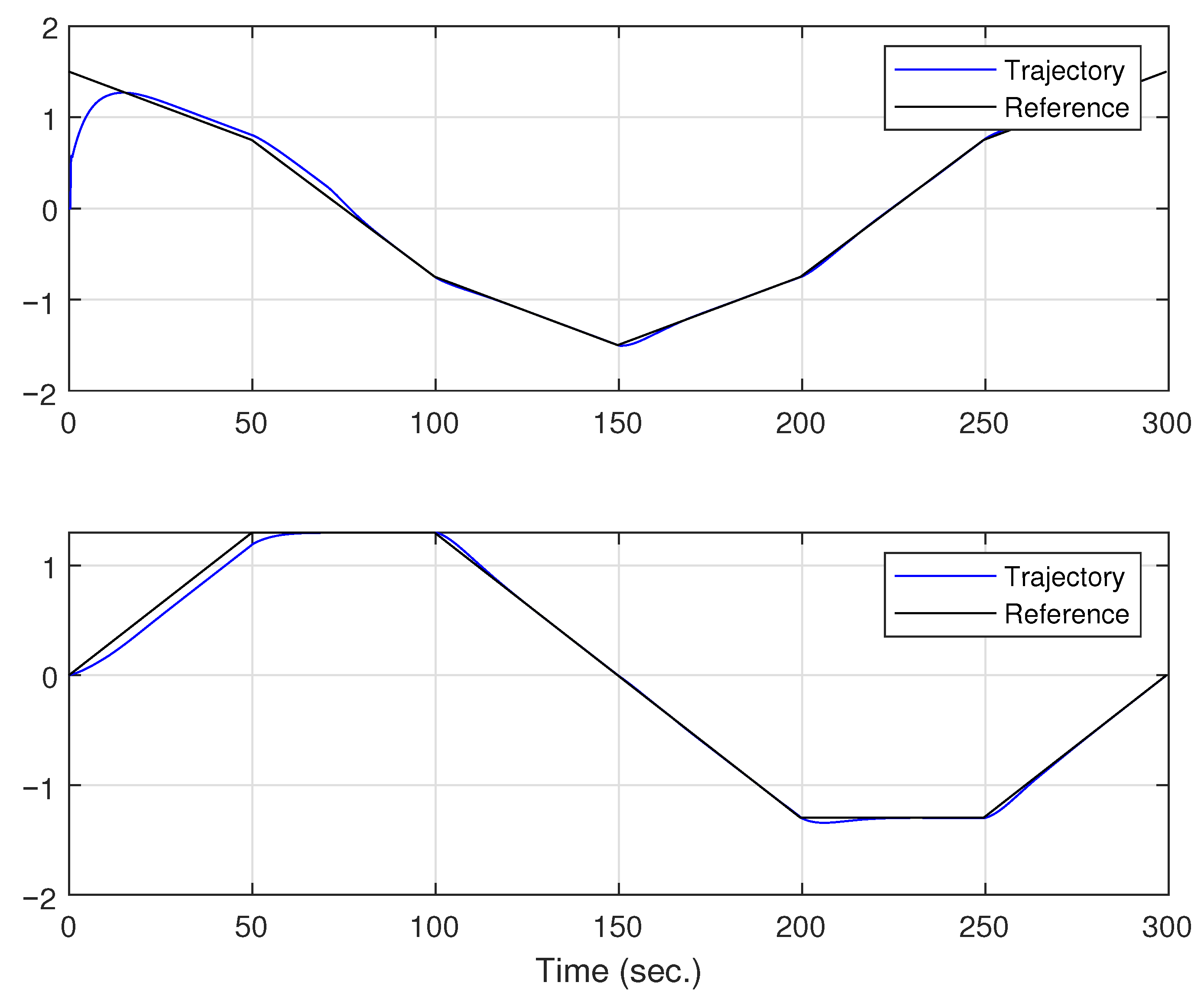
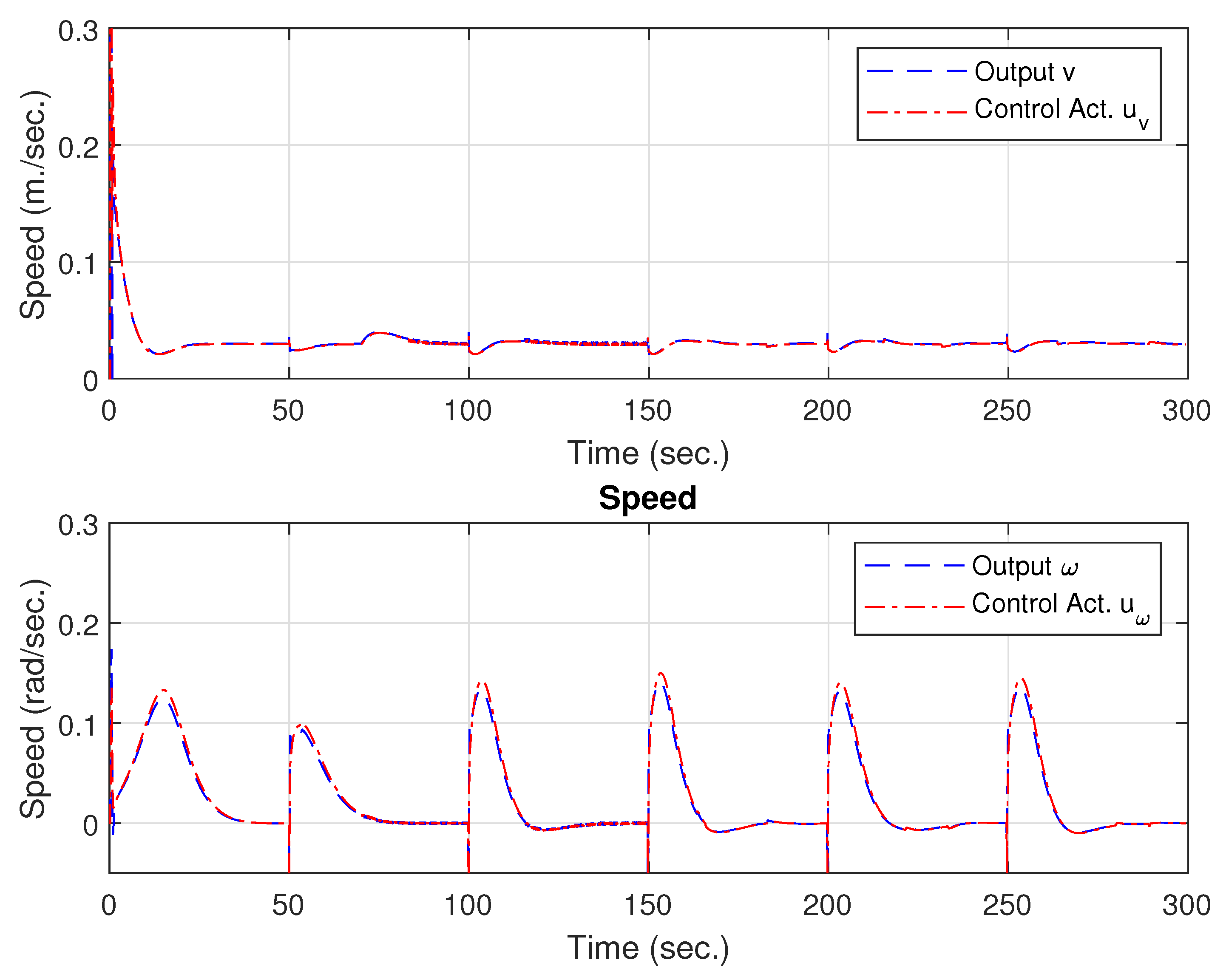
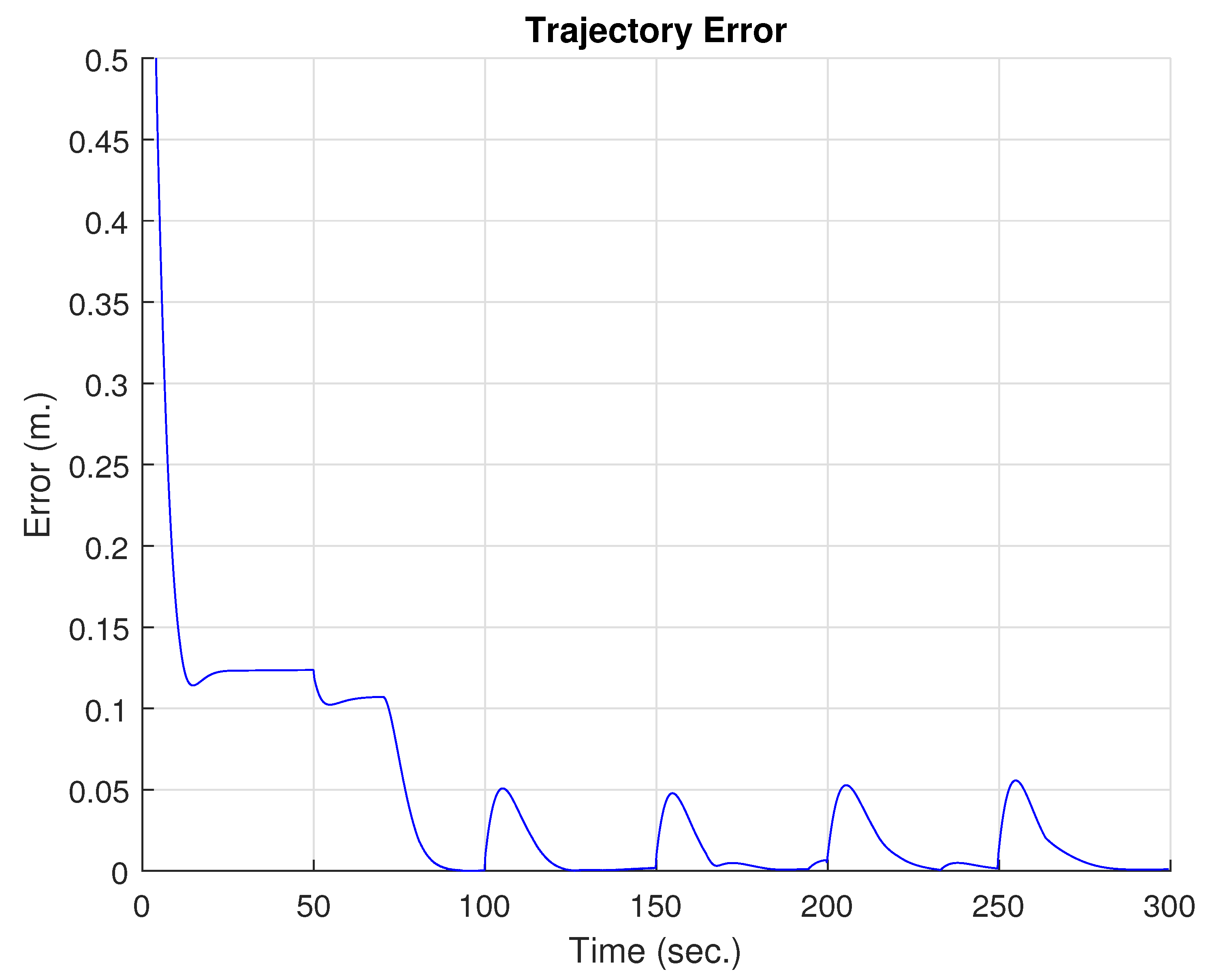
For the simulation experiment, WMR was considered for trajectory tracking. In this case, a hexagonal reference trajectory is established. To demonstrate the tracking capability with minimal error using the adaptive capacity of FLNNs, the dynamic parameters were altered by adding additional weight to the vehicle. This not only increases the mass, but also changes the center of gravity and increases friction due to deformation of the wheels. In the first few seconds, the robot operates with control without adaptive capability, where it can be observed in Figure 3 that the trajectory error is greater, including a peak in the first few seconds due to the WMR starting its trajectory away from the reference. Another point is Figure 4, where the upper subfigure indicates the position of the WMR on the x-axis, while the lower subfigure indicates the position of the WMR on the y-axis. After 75 s, the adaptive capability of the FLNN is activated, establishing a transient error that affects the trajectory. Seconds later, it can be observed that the error is considerably reduced, following the desired trajectory with greater fidelity than in the first few seconds. Figure 5 shows the vehicle’s speed control actions. The upper subfigure indicates the linear speed, where the vehicle follows the reference almost without any problems, except for the peak that occurs at 75 s due to the speed variation produced by the activation of the FLNN. The lower subfigure shows the angular velocity, revealing changes in velocity due to the small turns at each vertex of the trajectory. Finally, Figure 6 shows the mean square error produced by the proposed control technique, confirming the decrease in trajectory error after 75 s. In the experiment, it is easy to observe the reduction in trajectory error due to the activation of the neural network, which has the primary function of providing an adaptive characteristic to the proposed controller. Therefore, it adjusts the parameters of the FLNN neural network in the presence of dynamic uncertainties or external disturbances (the difference in error before and after 75 s shown in Figure 6).
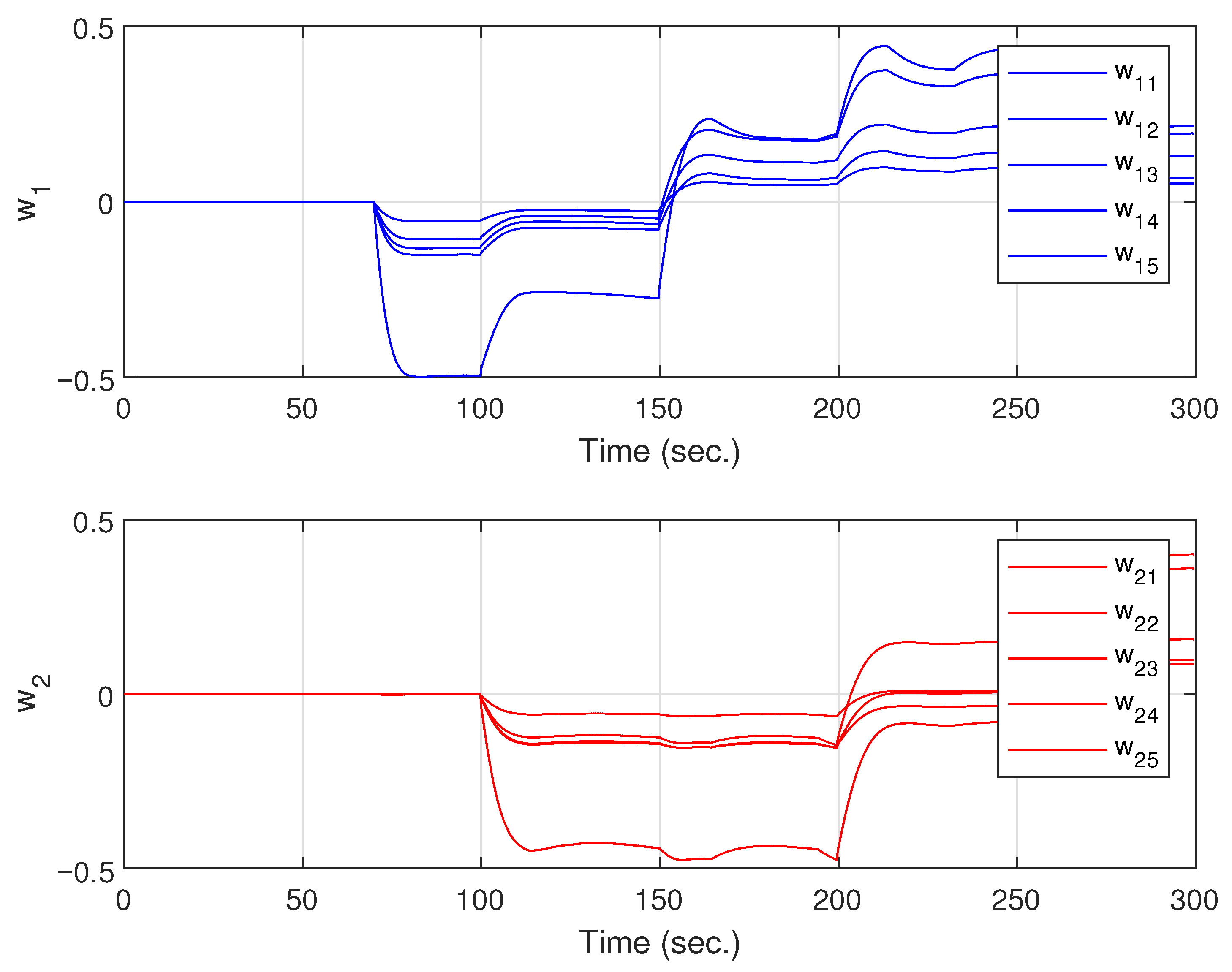
The last figure, Figure 7, shows the evolution of the weights of the FLNN output layer w . Where each subfigure shows the weights associated with each control action u v , u ω , it can be seen that the weights are bounded.
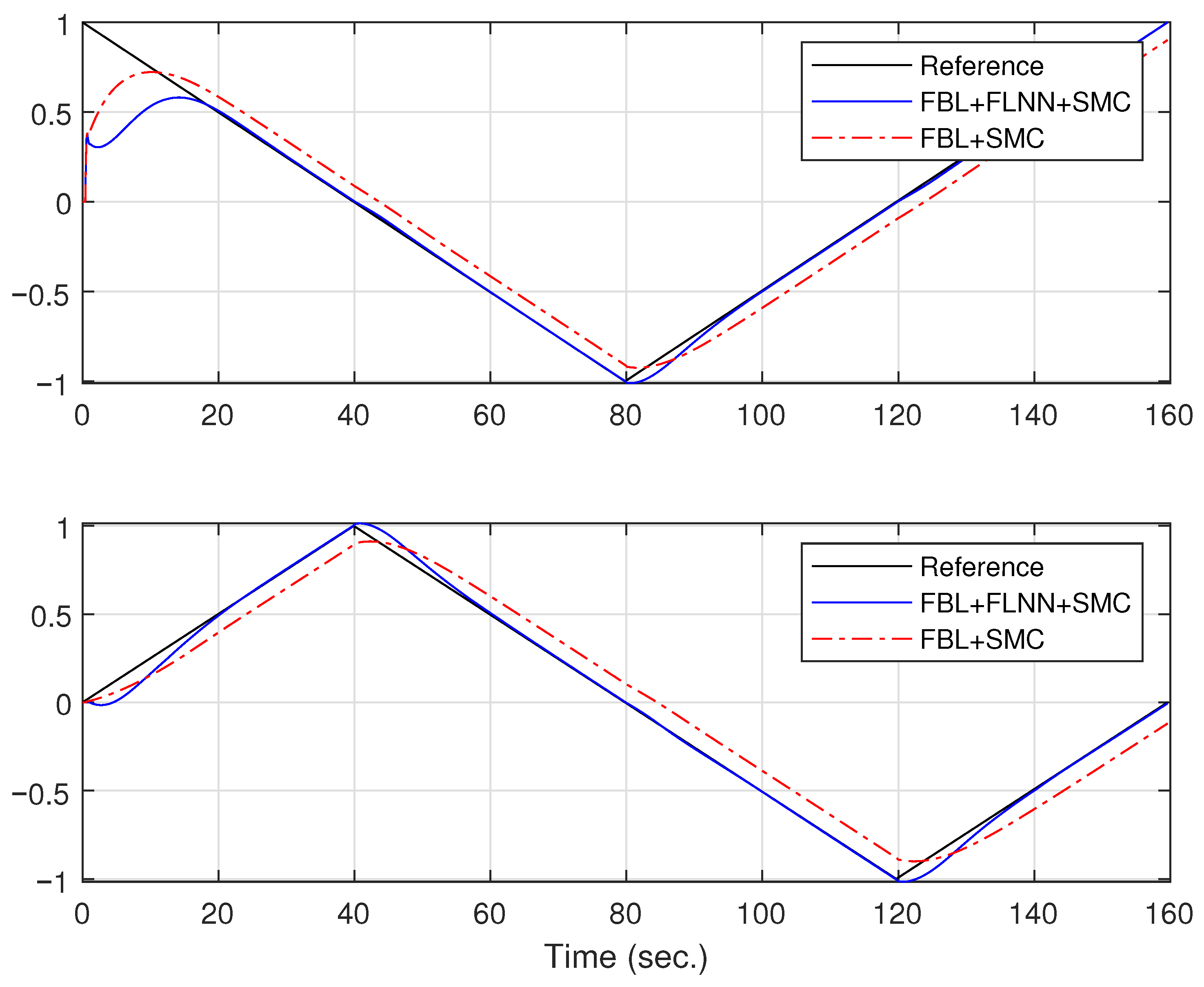
In the second experiment, a comparison is made between the proposed technique (feedback linearization (FLB) + SMC + FLNN) and the proposal without adaptive capacity (feedback linearization + SMC). Figure 8 shows the position of the WMR on the x- and y-axes. It can be seen that the proposed technique has a better response to trajectory tracking; in fact, it is easy to see that in both subfigures, the controller follows the desired trajectory more closely. It can also be seen in Figure 8 that the proposed controller has a better response to discontinuous trajectories (corners), attempting to reduce trajectory error more effectively.

7.2. Discussion

The proposed control technique shows favorable results for trajectory control for WMR. Although this technique was tested on WMR vehicles, it can be extended to other types of vehicles if part of their dynamic structure is known. Looking at the results, it can be said that dynamic control based on feedback linearization+SMC+FLNN can compensate for external disturbances acting on dynamics and kinematics, e.g., load variation, friction slip, etc. This technique can include unmodeled dynamics, where control was designed based on the reformulation of the known model of WMR dynamics (3). Another important consideration is that most controllers in the literature work very well with continuous trajectories (circles, ellipses, etc.) but fail or have large errors at points of discontinuity. The main idea was to demonstrate the robustness of the controller in the presence of trajectory discontinuities. Therefore, the main purpose of showing Figure 9 is to highlight how the controller behaves at sharper corners and that it does not lose the trajectory.
The results show the practical viability of the proposed control technique using FLNN, which can perfectly map uncertainties and disturbances. Future work will study its implementation in UAVs.

8. Conclusions

The objective of this work is to design a neuroadaptive SMC controller to reduce trajectory tracking error, which is applied to a WMR vehicle that has dynamic uncertainties. These uncertainties affect the correct tracking of the desired trajectory, which can be reduced with an appropriate control law. The proposed control technique is capable of generating smooth and continuous speed commands for the WMR with a small error compared to the SMC controller. The FLNN neural network reduces the difference between a known nominal dynamic structure and the dynamic structure of the WMR, which includes dynamic uncertainties. The results obtained with this technique are viable and can be applied to different vehicles with the same characteristics. The proposed control scheme is robust and guarantees the stability of the closed-loop system, being immune to different dynamic variations. It also presents a convergence towards zero of the tracking error. Future work will focus on experimental validation to further evaluate the applicability of the system and explore the adaptive adjustment of FLNN parameters in dynamic environments, where unmodeled external forces exist.

Author Contributions

Conceptualization, F.R., S.B., F.S.A., S.K., F.B. and J.G.; Data curation, S.K. and J.G.; Formal analysis, S.B. and F.R.; Funding acquisition, S.B.; Investigation, S.B., F.S.A., F.B. and E.Z.; Methodology, F.R.; Project administration, S.B.; Resources, S.B. and S.K.; Software, J.G.; Supervision, S.B. and F.R.; Validation, S.B., E.Z., F.B. and F.S.A.; Writing—original draft, F.R. and E.Z. Writing—review and editing, F.S.A. and F.B. All authors have read and agreed to the published version of the manuscript.

Funding

Deputyship for Research and Innovation, Ministry of Education in Saudi Arabia, project number MoE-IF-UJ-R2-22-20772-3.

Data Availability Statement

The original contributions presented in this study are included in the article. Further inquiries can be directed to the corresponding author.

Acknowledgments

The authors extend their appreciation to the Deputyship for Research and Innovation, Ministry of Education in Saudi Arabia, for funding this research work through the project number MoE-IF-UJ-R2-22-20772-3.

Conflicts of Interest

The authors declare no conflicts of interest.

Abbreviations

The following abbreviations are used in this manuscript:
WMRWheeled Mobile Robot
LABCLinear Algebra-Based Control
FOFractional Order
SMCSliding Mode Control (controller)
FLNNFunctional-Link Neural Network
AITSMCAdaptive Integral Terminal Sliding Mode Control
DOBCDisturbance-Observer-Based Control

Appendix A. Relative Degree

The relative degree r i of an output y i = h i ( x ) with respect to an input u j is the smallest integer k such that L g j L f k 1 h i ( x ) 0 , where L f h i ( x ) = h i x f ( x ) is the Lie derivative of h i along f ( x ) .
Calculation for y 1 = x 1
L f h 1 ( x ) = x 1 x f ( x ) = ( 1 , 0 , 0 , 0 , 0 ) f ( x ) = x 4 cos ( x 3 ) x 5 a sin ( x 3 ) .
L f 2 h 1 ( x ) = ( L f h 1 ( x ) ) x f ( x ) = ( 0 , 0 , x 4 sin ( x 3 ) x 5 a cos ( x 3 ) , cos ( x 3 ) , a sin ( x 3 ) ) f ( x ) =   = x 5 x 4 sin ( x 3 ) + x 5 a cos ( x 3 ) + + ϑ 3 ϑ 1 x 5 2 ( t ) ϑ 4 ϑ 1 x 4 cos ( x 3 ) ϑ 5 ϑ 2 x 5 x 4 ϑ 6 ϑ 2 x 5 a sin ( x 3 ) .
L g 1 L f h 1 ( x ) = ( 0 , 0 , x 4 sin ( x 3 ) x 5 a cos ( x 3 ) , cos ( x 3 ) , a sin ( x 3 ) ) 0 0 0 1 ϑ 1 0 = cos ( x 3 ) ϑ 1 .
L g 2 L f h 1 ( x ) = ( 0 , 0 , x 4 sin ( x 3 ) x 5 a cos ( x 3 ) , cos ( x 3 ) , a sin ( x 3 ) ) 0 0 0 0 1 ϑ 2 = a sin ( x 3 ) ϑ 2 .
Therefore, the relative degree is r 1 = 2 for u 1 and r 1 = 2 for u 2 .
Calculation for y 2 = x 2
L f h 2 ( x ) = x 2 x f ( x ) = ( 0 , 1 , 0 , 0 , 0 ) f ( x ) = x 4 sin ( x 3 ) + x 5 a cos ( x 3 ) .
L f 2 h 2 ( x ) = ( L f h 2 ( x ) ) x f ( x ) = ( 0 , 0 , x 4 cos ( x 3 ) x 5 a sin ( x 3 ) , sin ( x 3 ) , a cos ( x 3 ) ) f ( x ) =   = x 5 x 4 sin ( x 3 ) + x 5 a cos ( x 3 ) + + ϑ 3 ϑ 1 x 5 2 ϑ 4 ϑ 1 x 4 sin ( x 3 ) + ϑ 5 ϑ 2 x 5 x 3 ϑ 6 ϑ 2 x 5 a cos ( x 3 )
L g 1 L f h 2 ( x ) = ( 0 , 0 , x 4 cos ( x 3 ) x 5 a sin ( x 3 ) , sin ( x 3 ) , a cos ( x 3 ) ) 0 0 0 1 ϑ 1 0 = sin ( x 3 ) ϑ 1 .
L g 2 L f h 2 ( x ) = ( 0 , 0 , x 4 cos ( x 3 ) x 5 a sin ( x 3 ) , sin ( x 3 ) , a cos ( x 3 ) ) 0 0 0 0 1 ϑ 2 = a cos ( x 3 ) ϑ 2 .
The relative degree is r 2 = 2 for u 1 and r 2 = 2 for u 2 . The decoupling matrix for the second derivatives is
B ( x ) = cos ( x 3 ) ϑ 1 a sin ( x 3 ) ϑ 2 sin ( x 3 ) ϑ 1 a cos ( x 3 ) ϑ 2 .
This matrix is invertible, which indicates that we can completely linearize the system without restrictions on the second derivatives.

Appendix B

The mobile robot parameters are described by
ϑ 1 = ( R a k a ) ( M R t r w + 2 I e + 2 r w k d t ) 2 r w k p t ϑ 2 = ( R a k a ) ( I e d 2 + 2 R t r w ( I z + M b 2 ) ) + 2 r w d k d r T 2 r w k p r ϑ 3 = ( R a k a ) ( M b R t ) 2 k p t ϑ 4 = ( R a k a ) ( k a k b R a + B e ) r w k p t + 1 ϑ 5 = ( R a k a ) ( M b R t ) k p r ϑ 6 = ( R a k a ) k a k b R a + B e d 2 r w k p t + 1  
In these relations, M is the robot mass;
  • r w is the radius of the left and right wheels;
  • k b is equal to the electro motoric force constant multiplied by the reduction constant;
  • R a is the electric resistance;
  • k a is the constant of torque multiplied by the reduction constant;
  • k p r , k p t , and k d t are positive constants;
  • I e is the moment of inertia (electric actuator);
  • B e is the viscous friction coefficient (electric actuator);
  • R t is the nominal radius of the wheel.

References

  1. Wit, C.C.d.; Khennouf, H.; Samson, C.; Sordalen, O.J. Nonlinear control design for mobile robots. In Recent Trends in Mobile Robots; World Scientific: Singapore, 1993; pp. 121–156. [Google Scholar]
  2. Patiño, K.; Slawiñski, E.; Moran-Armenta, M.; Mut, V.; Rossomando, F.G.; Moreno-Valenzuela, J. Neural Networks in the Delayed Teleoperation of a Skid-Steering Robot. Mathematics 2025, 13, 2071. [Google Scholar] [CrossRef]
  3. Xu, J.X.; Guo, Z.Q.; Lee, T.H. Design and implementation of integral sliding-mode control on an underactuated two-wheeled mobile robot. IEEE Trans. Ind. Electron. 2013, 61, 3671–3681. [Google Scholar] [CrossRef]
  4. Zhang, Z.; Wen, C.; Xing, L.; Song, Y. Adaptive output feedback control of nonlinear systems with mismatched uncertainties under input/output quantization. IEEE Trans. Autom. Control 2022, 67, 4801–4808. [Google Scholar] [CrossRef]
  5. Zheng, B.C.; Park, J.H. Sliding mode control design for linear systems subject to quantization parameter mismatch. J. Frankl. Inst. 2016, 353, 37–53. [Google Scholar] [CrossRef]
  6. Ma, Y.; Liu, L.; Zhu, C.; Liu, Y.; Zeng, Q. Robust Safety Critical Control for Nonholonomic Wheeled Mobile Robot Trajectory Tracking with Matched Disturbance. In Proceedings of the 2024 IEEE 8th International Conference on Vision, Image and Signal Processing (ICVISP), Kunming, China, 27–29 December 2024; pp. 1–5. [Google Scholar] [CrossRef]
  7. Yu, X.; Yu, X. Brain-Controlled Wheeled Mobile Robots: A Framework Combining Probabilistic Brain–Computer Interface and Model Predictive Control. IEEE Trans. Cybern. 2025, 55, 4311–4321. [Google Scholar] [CrossRef] [PubMed]
  8. Zhang, Y.; Zhao, B.; Liu, D. Distributed Optimal Containment Control of Wheeled Mobile Robots via Adaptive Dynamic Programming. IEEE Trans. Syst. Man Cybern. Syst. 2025, 55, 5876–5886. [Google Scholar] [CrossRef]
  9. Hasanlu, M.; Siavashi, M. Fuzzy adaptive back stepping control of wheeled mobile robot. Robot. Syst. Appl. 2025, 5, 12–27. [Google Scholar] [CrossRef]
  10. Mondal, S.; Verma, G.K.; Ray, R.; Vadali, S.R.K.; Aruchamy, S.; Nandy, S. Polynomial Based Intelligent Path-following Control Scheme for Nonholonomic Mobile Robots: Theory and Experiments. Int. J. Control. Autom. Syst. 2025, 23, 2117–2131. [Google Scholar] [CrossRef]
  11. Guo, J.; Luo, Y.; Li, K. Adaptive neural-network sliding mode cascade architecture of longitudinal tracking control for unmanned vehicles. Nonlinear Dyn. 2017, 87, 2497–2510. [Google Scholar] [CrossRef]
  12. Martins, F.N.; Celeste, W.C.; Carelli, R.; Sarcinelli-Filho, M.; Bastos-Filho, T.F. An adaptive dynamic controller for autonomous mobile robot trajectory tracking. Control Eng. Pract. 2008, 16, 1354–1363. [Google Scholar] [CrossRef]
  13. Filipescu, A.; Solea, R.; Stamatescu, G.; Ciubucciu, G. Trajectory-Tracking Sliding-Mode Control of the Autonomous Wheelchair Modeled as a Nonholonomic WMR. In Proceedings of the 2018 IEEE 14th International Conference on Control and Automation (ICCA), Anchorage, AK, USA, 12–15 June 2018; pp. 1168–1173. [Google Scholar]
  14. Yang, L.; Pan, S. A Sliding mode control method for trajectory tracking control of wheeled mobile robot. J. Phys. Conf. Ser. 2018, 1074, 012059. [Google Scholar] [CrossRef]
  15. Gao, H.; Song, X.; Ding, L.; Xia, K.; Li, N.; Deng, Z. Adaptive motion control of wheeled mobile robot with unknown slippage. Int. J. Control 2014, 87, 1513–1522. [Google Scholar] [CrossRef]
  16. Park, B.S.; Yoo, S.J.; Park, J.B.; Choi, Y.H. Adaptive neural sliding mode control of nonholonomic wheeled mobile robots with model uncertainty. IEEE Trans. Control Syst. Technol. 2008, 17, 207–214. [Google Scholar] [CrossRef]
  17. Shojaei, K.; Shahri, A.M.; Tarakameh, A.; Tabibian, B. Adaptive trajectory tracking control of a differential drive wheeled mobile robot. Robotica 2011, 29, 391–402. [Google Scholar] [CrossRef]
  18. Tran, D.L.; Cao, N.T.D.; Phan, V.D.; Duong, D.T.; Ho, S.P. Advanced trajectory tracking control for wheeled mobile robots under actuator faults and slippage. Bull. Electr. Eng. Inform. 2025, 14, 1746–1757. [Google Scholar] [CrossRef]
  19. Scaglia, G.; Montoya, L.Q.; Mut, V.; di Sciascio, F. Numerical methods based controller design for mobile robots. Robotica 2009, 27, 269–279. [Google Scholar] [CrossRef]
  20. Petrov, P.; Kralov, I. Exponential Trajectory Tracking Control of Nonholonomic Wheeled Mobile Robots. Mathematics 2025, 13, 1. [Google Scholar] [CrossRef]
  21. Labbadi, M.; Boubaker, S.; Djemai, M.; Mekni, S.K.; Bekrar, A. Fixed-time fractional-order global sliding mode control for nonholonomic mobile robot systems under external disturbances. Fractal Fract. 2022, 6, 177. [Google Scholar] [CrossRef]
  22. Phan, V.D.; Ho, S.P.; Dang, T.S.; Le, V.C.; Dinh, V.N. Development of an Adaptive Integral Terminal Sliding Mode Tracking Control for a Wheeled Mobile Robot with Time Delay Estimation. Int. J. Control. Autom. Syst. 2025, 23, 2399–2410. [Google Scholar] [CrossRef]
  23. Ioannou, P.A.; Sun, J. Robust Adaptive Control; PTR Prentice-Hall: Upper Saddle River, NJ, USA, 1996; Volume 1. [Google Scholar]
  24. De La Cruz, C.; Carelli, R. Dynamic modeling and centralized formation control of mobile robots. In Proceedings of the IECON 2006-32nd Annual Conference on IEEE Industrial Electronics, Paris, France, 6–10 November 2006; pp. 3880–3885. [Google Scholar]
  25. Khalil, H.K. Nonlinear Systems; Prentice Hall: Upper Saddle River, NJ, USA, 2002. [Google Scholar]
  26. Polycarpou, M.M. Stable adaptive neural control scheme for nonlinear systems. IEEE Trans. Autom. Control 2002, 41, 447–451. [Google Scholar] [CrossRef]
  27. Shtessel, Y.; Edwards, C.; Fridman, L.; Levant, A. Sliding Mode Control and Observation; Springer: New York, NY, USA, 2014; Volume 10. [Google Scholar]
  28. Lewis, F.L.; Jagannathan, S.; Yesildirak, A. Neural Network Control of Robot Manipulators and Non-Linear Systems; CRC Press: Philadelphia, PA, USA, 1999. [Google Scholar]
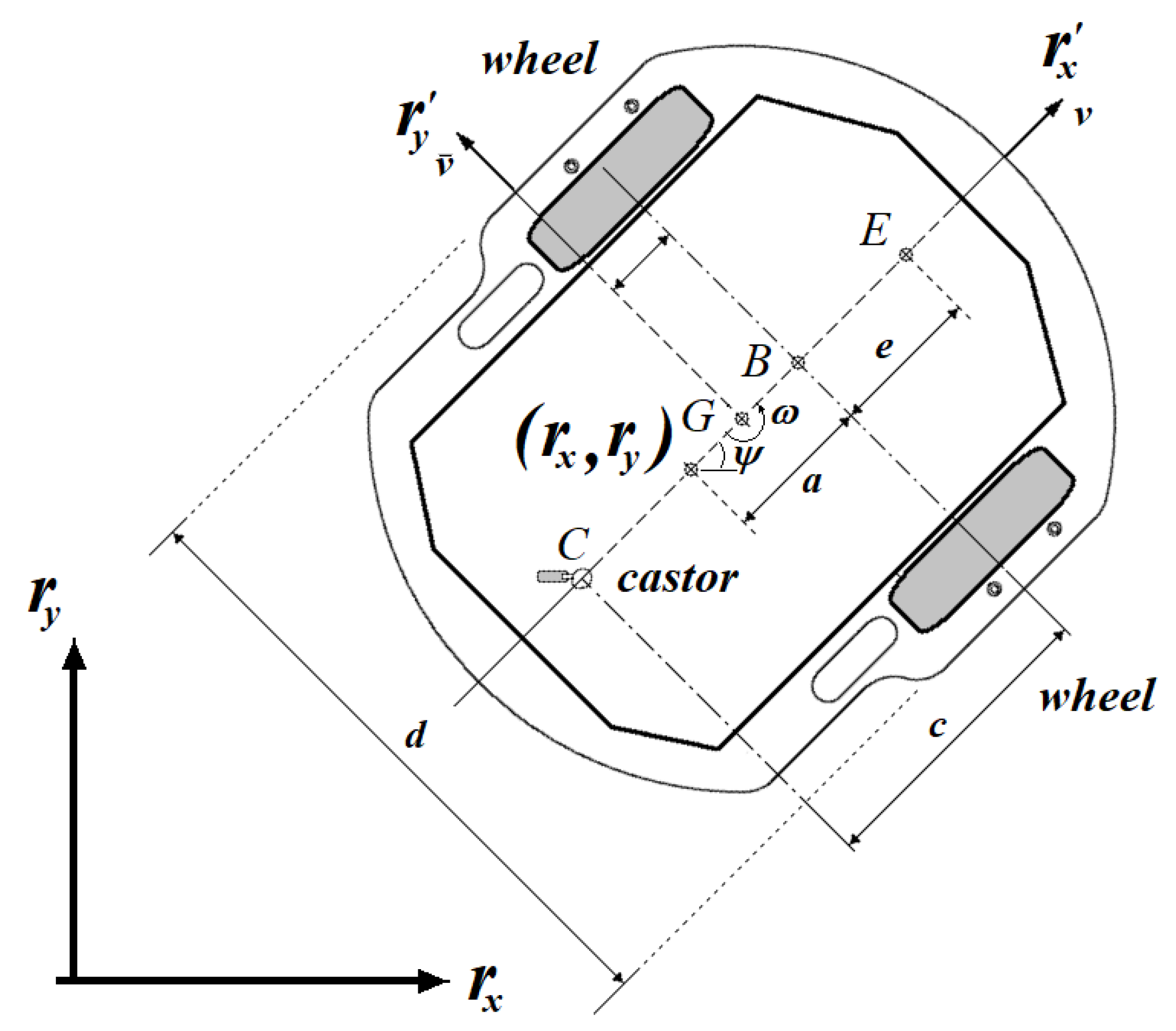
Figure 1. Mobile robot parameters.
Mathematics 13 03178 g001
Figure 2. Proposed control structure.
Mathematics 13 03178 g002
Figure 3. Reference trajectory and actual trajectory followed by the WMR; the solid black line indicates the desired trajectory and the blue dashed line indicates the actual trajectory followed by the robot.
Mathematics 13 03178 g003
Figure 4. The upper subfigure indicates the position of the WMR on the x-axis, while the lower subfigure indicates the position of the WMR on the y-axis.
Mathematics 13 03178 g004
Figure 5. WMR output speeds ( v , ω ) and control actions ( u v , u ω ).
Mathematics 13 03178 g005
Figure 6. Mean square error of trajectory tracking.
Mathematics 13 03178 g006
Figure 7. Weight evolution during trajectory tracking.
Mathematics 13 03178 g007
Figure 8. Position of the WMR in x- and y-axes, respectively.
Mathematics 13 03178 g008
Figure 9. Comparison of the trajectories followed by the WMR with and without FLNN.
Mathematics 13 03178 g009
Table 1. Identified parameters for Pioneer DX2 mobile robot.
ϑ 1 ϑ 2 ϑ 3 ϑ 4 ϑ 5 ϑ 6
0.30370.2768−0.00040180.9835−0.0038181.0725
Disclaimer/Publisher’s Note: The statements, opinions and data contained in all publications are solely those of the individual author(s) and contributor(s) and not of MDPI and/or the editor(s). MDPI and/or the editor(s) disclaim responsibility for any injury to people or property resulting from any ideas, methods, instructions or products referred to in the content.