1. Introduction
Bots and robotic agents have been known to masquerade as humans [
1] for decades. By now, over 80% [
2] of traffic targeting public-facing interfaces is generated by bots. While some introduce themselves as bots and serve practical purposes or at least give the operator the option to serve or block them, others hide and consume resources reserved for human visitors. Also, some are outright abusive. Their abusiveness spans a broad spectrum, from penetration testing to engaging in intellectual property theft.
While real-time bot detection systems exist, they either work off fixed rules like IP address range classification [
3] or send extra traffic fingerprint metadata [
4] to an off-site service. The former is ineffective, and the latter adds precious seconds to the content delivery pipeline. It must not be forgotten that the final goal is to provide the best user experience to the end user and not to find and block each bot. Therefore, it can be beneficial to pre-classify data streams according to their statistical bot penetration and provide them with appropriate strength filters. The existing computationally expensive validations become feasible when applied to a narrow set, especially when the cleanest traffic bypasses deep analysis and is served with the lowest latency.
In a broader sense, our goal is to provide a simple database lookup to pre-classify traffic flows.
We will show that this pre-sorting is possible using a transformer-based classifier.
We will show that training of such a classifier requires baseline human and bot behavior that we will obtain from behavioral simulation and real traffic data.
We will validate the classifier with yet unseen real-life traffic data.
We will also show that this method allows service operators to move away from reactive blocking to proactive resource management and service tuning.
2. Previous Work
Current academic research focuses on accurate bot detection at “all costs”. Boujrad, A. et al. [
5] contrast known browser fingerprints with the same user-agent data obtained from honeypot logs, and Iliou, C. et al. [
6] monitor behavioral biometrics like mouse movement. Both methods require real-time monitoring and data transmission to third-party services, which may not be viable under current privacy regulations, given the extra metadata included. Similarly to what we propose, Zeng, X. et al. [
7] trained models to detect evolving spoofing behaviors, including user-agent manipulation, although primarily for social networks and on synthetic data.
Another avenue of research is the integration of botnet detection into wider, often multimodal frameworks as proposed by Robert, B. [
8]. These may include bot metrics as part of the global threat score, performing multiple checks in parallel, thus making a single go/no-go decision less transparent, like Neural Network-driven solutions. Recognizing this, Saied, M., & Guirguis [
9] researched methods to make AI-based bot detection methods more transparent and performance-friendly, extracting decision rules from the network and using those in the detection framework directly. Like our proposal, this makes the pre-classification of robotic agents quick, less CPU-intensive, and viable in high-traffic volume scenarios.
Another promising avenue is detecting and analyzing the content bots push to or retrieve from online services. This differs from biometric metadata, but it is metadata nevertheless. Therefore, it can be analyzed to improve standalone methods’ accuracy or increase the feature vector of AI-based methods as described by Zhou, M. et al. [
10]. While this has mainly been perfected in social networks, like in the work of Arranz-Escudero, O. et al. [
11], it is a promising way forward for most abusive or exploitative bots.
Our approach is to unify the best aspects of previous methods, including conformance to current privacy standards (no outgoing metadata), the “C” column in
Table 1, rule-based, quick, and transparent decision-making (“D” column). We also target easy availability for all online service types (“S” column), without requiring third-party input like biometrics (“B” column). Our tradeoff is that we do not inspect each transaction independently, but as a batch, with the agent string being the grouping factor. Thus, instead of a bot/nobot decision, we provide a probabilistic botness metric that can be used as input for further processing, either by a network or an application firewall, or as a selection criterion for differentiated quality or service pipelines.
3. Materials and Methods
3.1. Glossary
To improve clarity and consistency,
Table 2 summarizes the key variables and symbols used throughout the modeling framework. All variables are defined as they appear in the equations, pseudo-codes, and plots below.
3.2. Data and Feature Set
From 2019 to 2023, we collected data for over 600 million online service requests from 4000 domains. The AGWA [
12] set provides the big-data foundation for this work. Importantly, the raw data structure follows the standard Apache web server log [
13] for this method to be available for the broadest audience. The structure is shown in
Table 3.
The simplicity of the dataset is key to our ability to collect it in a standardized format from multiple sources for later consolidation. Another advantage is that these records are all available from the same application within the content delivery process. Thus, they can be collected from a single infrastructure layer instead of different features having to be correlated across heterogeneous environments, like in the case of most biometric or application/UI fingerprint methods.
We grouped the original data into separate files (learning sets) organized by the user-agent string. The user-agent string is distinctive in the sense that while its use is not standardized, a particular string’s prevalence in the logs must correlate to its agent’s popularity. With the current web browser auto-deployment and updating schemes, this popularity follows a well-established schedule and is not simply a user preference.
Table 4 shows the feature vectors (
) that we established for each user-agent in our learning sets.
While we are confident that our method works well globally, a network trained on data obtained from European servers would work well for classification on an Asian server; we allow for local variations by embedding local information in the feature set. The regional information in our case comes from an external lookup table that identifies local visits to the monitored sites based on the source IP. Knowing, for example, that the data had been collected in Hungary on sites intended for a Hungarian audience, we include the metric P(Local_Source) indicative of the intended Hungarian visitor type.
While this provides enhanced detection, it also allows the implementation of the method for different operators in different geographical regions, using the same core data but extracting a more relevant ruleset for their specific situation.
3.3. Transformer Classifier
We aim to determine the amount of bot contamination of a specific user-agent string based on temporal feature vector trends. That is, we are not looking at determining whether a user agent is a bot; instead, we assume it is a mixture of genuine human and robotic traffic. We also understand that the ratio may change over time, and we are interested in the current value. To achieve this, we must train the network with baseline human and robotic traffic data. Both are challenges for which we present a solution in the following chapters.
For the network, we selected a transformer-based classifier architecture, following the principles outlined by Terechshenko et al. [
14], demonstrating that transformers are particularly well-suited to handle structured but noisy or irregular time series data. This model’s self-attention mechanism enables it to prioritize salient patterns across varying temporal scales—an essential property for our application, where user-agent traffic may be sporadic and heavily imbalanced over time. In our case, the underlying structure is defined by daily user-agent progression, and the model must learn to distinguish subtle bot-like deviations.
Training is performed on fixed-length, 30-day data windows [
15], that we extracted from labeled data sequences. To ensure fairness across agents of varying traffic strength, we apply logarithmic weighting (based on all hits attributed to the specific agent-string) to all training windows and normalize all evaluation metrics. Since the model uses a SoftMax [
16] output layer during evaluation, the agent scoring will be on a full probabilistic range.
Our design for the classification is outlined in Algorithm 1.
| Algorithm 1 Pseudo code of the Transformer based Classification |
1: For each file in data_dir: do
2: Assign pre-determined bot label ← 1 or 0
3: Read file in SEQ_LEN steps (step numbers <= MAX_WND) and Extract to []features
4: For all SEQ_LEN steps: do
5: total_hits ← sum of traffic_hits
6: weight ← log(1 + total_hits)
7: Add ([]features, label, weight) to training_samples
8: For all epoch in range(EPOCHS): do
9: Set model to train mode
10: For all (([]features, label, weight) in training_samples:
11: pred ← model([]features)
12: base_loss ← CrossEntropyLoss(reduction = ‘none’)(pred, label)
13: weighted_loss ← mean(base_loss * weight)
14: optimizer.zero_grad()
15: weighted_loss.backward()
16: optimizer.step()
Meta parameters:
Parameters:
|
As seen in Algorithm 1, the classification requires pre-tagged data for human and bot activity patterns, which is one of the project’s main challenges. While we detail the acquisition of such sets in the following chapters, it is essential to note that a third independent set is also needed to test the resulting classification and evaluate it against our expectations, so that we can judge the effectiveness before we apply it against third-party datasets.
3.4. Protection Against Overfitting
, and values had been tuned explicitly against overfitting. At it is in the same order as , and both the attention heads and depth are kept light when contrasted with the number of training samples: , in the 20,000 range.
To assess generalization and make the risk of overfitting visible, we adopted a 10% holdout strategy. Specifically, the dataset of user-agent progressions was randomly partitioned so that 90% of the sequences were used for model training and the remaining 10% were reserved exclusively for evaluation. During training, the holdout sequences were never seen, ensuring that performance metrics reflect the model’s ability to generalize to new, independent progressions.
3.5. Theoretical Justification of Weighting Scheme in Bot Training
Let Equation (1) denote the total number of hits observed for agent
If raw frequencies were used directly as weights, high-traffic agents (popular search engines) would dominate training, leading to biased optimization. However, using uniform weights would disregard the reliability of larger samples. To balance these extremes, we apply a logarithmic transformation as described by Equation (2):
This follows the general principle of sublinear frequency scaling, ensuring that relative differences between agents are preserved while preventing unbounded dominance of high-volume progressions. In terms of information theory, expressed like this also approximates the expected entropy contribution of agent as the amount of new information gained from additional observations is proportional to . In contrast, linear weighting can cause memorization of a few high-traffic agents, yet uniform weighting understates credible patterns present in larger samples. Consequently, log weighting yields a balanced influence across agents of different scales. We also note that the logarithmic form was selected for its simplicity: unlike alternative sublinear weighting schemes, which require either a threshold or a tuning parameter.
3.6. Complexity Analysis of Training Procedure
The training is designed to run as often as new logs become available. This is once daily for most systems, but some might argue that even an hourly re-evaluation of the agents might bring additional benefit. Therefore, knowing the complexity of the training and being able to cap it is significant.
Each agent has a different amount of data available, but
caps the number of
size sliding windows, we process; therefore, we can safely estimate the order of the total number of training samples for
agents as in Equation (3):
Each sample is processed by a Transformer encoder of depth:
, embedding dimension:
, and attention heads:
. This leads to a sample processing complexity as shown by Equation (4)
The total complexity is the product of Equations (3) and (4) and scales quadratically with the SEQ_LEN. That is why fixing it to the lowest meaningful value (time period of 30 days) is essential.
3.7. Bot Training Set Tagging
We first tagged a subset of the AGWA progressions as bots (.bot) to prepare the training and evaluation sets. This tagging was based on tangential RFC 9309 [
17] compliance: user-agent strings explicitly identifying themselves as automated tools, such as those containing the keywords “bot,” “spider,” or “crawler”, were labeled as bots.
From the remaining user-agent strings, we selected those that contained the “Chrome” designator but not previously tagged as bots. These progressions formed our third test set for subsequent evaluation (.chrome).
All other unclassified user-agents were subjected to our behavioral modeling and trust-scoring pipeline. The 200 most human-like progressions, based on similarity to modelled browser lifecycle decay patterns, were selected and tagged as human to complete the training dataset. In other words, although we merely modelled human behavior, we did use real-life data for the training, those sets that matched our models the best.
The AGWA dataset contains temporal traffic profiles for approximately 2.2 million distinct user-agent strings. To ensure the quality and consistency of our feature extraction and model training, we restricted our selection to agents with at least 30 days of data and a minimum of 5000 total recorded requests.
Notably, the 30-day minimum sequence length directly influenced the design of our transformer classification network in the creation of the 30-day training and evaluation windows.
3.8. Quantitative Human Training Set Identification
The training process needs human training data or data with a minimum level of bot contamination for successful classification. We work under the assumption that the AGWA dataset has such progressions, and we can find them through empirical modelling and selecting sets closest to the model result. In our previous work [
18], we derived the average human-like progression by aggregating many progressions that fit a specific centroid filter.
3.9. Centroid Filter to Eliminate Bot-like Web Traffic
Based on our extensive industry experience, we first developed a tunable quantitative filtering process to eliminate temporal progressions that do not follow our expectation that a specific browser version peaks in popularity around the day index of the regular update cycle. Our centroid filter favors temporal progressions where the activity centers around a regular update period and can penalize progressions that decay at a rate or slower than a linear profile.
The centroid filter evaluation formula is captured by Equation (5).
It processes day indices for the first 2 years of observations and accepts calculated values between and . For our study, we used and values to block only the most obviously non-human progressions. The qualifying agents were stacked against matching day index values.
Stacking of all such qualifying
agent progressions are formulated by Equation (6) as
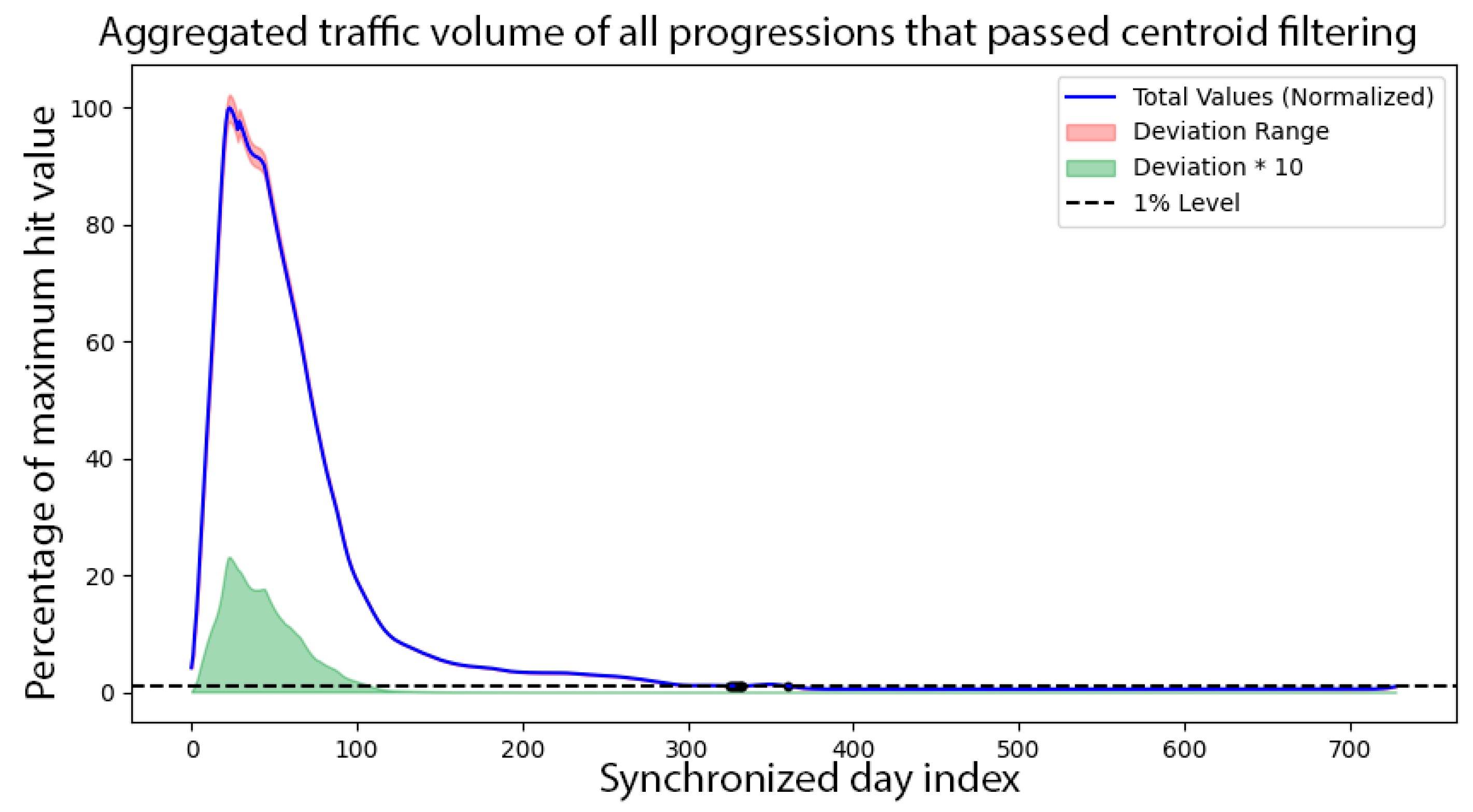
The normalized stacked progression is our quantitative base progression model, shown in
Figure 1. The maximum value is 100%, and all other values are scaled linearly.
Based on these findings, our goal was to build a tunable behavioral model that replicated this double-peak behavior, which is our best data-based model of a browser version’s traffic distribution during its lifecycle, free from bot and robotic agent effects.
3.10. Behavioral Model-Based Human Training Set Identification Refinement
We aim to model a “true-to-life” environment that considers current auto-deploy and update strategies of modern browsers. We initialize a population that all have version 0 (v0) browsers. Updates are pushed out to the population every () days. Once a new version is out, users update at () percentage daily per the strategy outlined in “Meta parameters”. There is an initial burst update period of () days with an added update ratio of () percentage. Users who demonstrated a previous reluctance to upgrade would continue updating at a rate reduction of () per the strategy outlined in “Meta parameters”. The population is expanding at the () rate, and planned obsolescence is at ().
Our complete simulation algorithm is described by Algorithm 2.
| Algorithm 2 Pseudo code of the Behavioral modelling |
1: Create initial population: All users start at version 0.
2: For each day from 1 to DAY_MAX do:
3: Determine the current browser release version (based on release cycle: B_RC)
4. For all browser version:
5: If the version is older than the current release: then
6: Calculate update chance (as per meta parameters)
7: Update browser to the current version at calculated rate
8: Simulate defunct users: (UPD_STOP) stop updating
9: Simulate population expansion: (UPD_EXP) born on the current version
Meta parameters:
: starting 15%/day, decreasing by 1% each day, min 1%
|
3.11. Simulation Meta Parameter Selection and Real-World Connection
To ensure that our human-traffic progression model is grounded in real-world browser behavior and not based on opportunistic parameter choices, we selected meta-parameters that reflect documented browser update dynamics when the AGWA dataset was collected. Google Chrome historically operated on a six-week major release cycle until its shift to a four-week cycle in late 2021 [
19]. Equally important, auto-update rollouts typically occur over about 7–10 days in a staggered fashion across the user base, a strategy multiple platforms use to balance update speed and stability.
In our model, the parameters representing update rate, burst period, and decay dynamics are calibrated to mimic these real-world processes. Release cycle and update rate capture the timing and shape of progressive adoption peaks—especially the significant uptake within the first 7–10 days—which similarly governs the decay of previous versions.
This model aims to estimate the timing and decay speed of browser version adoption down to the 1% prominence level. We then approximate this behavior with an anchored exponential decay. As such, none of the individual parameters can be finely tuned to force a specific outcome; rather, they collectively approximate the general lifecycle behavior observed in practice.
3.12. Simulation Results and Further Processing
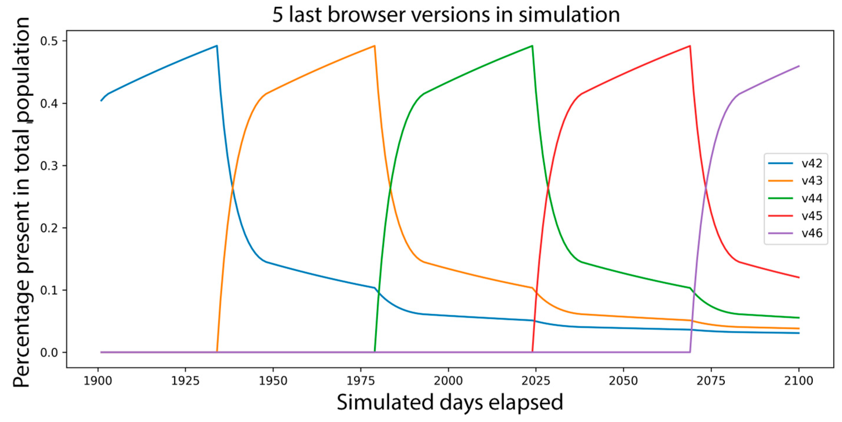
After simulating
days, the resulting browser version distribution has already stabilized. The results of the last five versions are shown in
Figure 2. We use v43 as the baseline against which we evaluate the real data progressions.
Given that the
meta parameter governs the distance of the peaks and the decay slope; direct comparison to real-life progressions must be preceded by linearly scaling and resampling the live data. The first anchor point of the scale is the maximum day index, and the second is where the progression drops below 1% of the maximum value. To account for the fact that the real data is noisy and possibly sparse, we will first fit an anchored exponential + constant curve over the data with minimum MSE and use that to estimate the 1% drop-off day index. Scaling and resampling are described in Algorithm 3.
| Algorithm 3 Model fitting and divergence metrics from real data |
1: Find V43 population maximum and THRESHOLD dropoff day boundary indexes
2: Normalize V43 population to/for 1.0 maximum value
3: For all candidates (.pothuman), temporal progression data files: do
4: day_index and traffic volume data are read
5: Fill in gaps using linear interpolation between existing points
6: Apply a 7-day moving average to reduce noise (for maximum detection only)
7: Locate the day_index with maximum smoothed traffic
8: Trim data to keep only those from the peak day onward.
9: Fit anchored exponential + constant model to raw maximum with MSE
10: Predict drop-under-THRESHOLD day_index
11: Rescale and resample the candidate curve
12: Normalize resampled candidate curve to/for 1.0 maximum value
13: Compute MSE between normalized MSE and V40
14: Find the SAM_HUM smallest MSE progressions for tagged human sample training
Meta parameters
|
Comparing the drop-off and its anchored exponential approximation, especially, allows us to eliminate noise from sparse data and occasional data processing quirks inherent to the AGWA dataset. Using this approximation is justified because after the maximum acceptance of a specific browser version, they should exhibit a close to exponential decay phase as seen in Equation (7).
This form arises naturally from first-order decay processes in population dynamics, where the probability of “survival” of a version decreases proportionally to its current usage. The fitted parameters have physically interpretable meaning: peak adoption level, decay rate, and residual share, respectively.
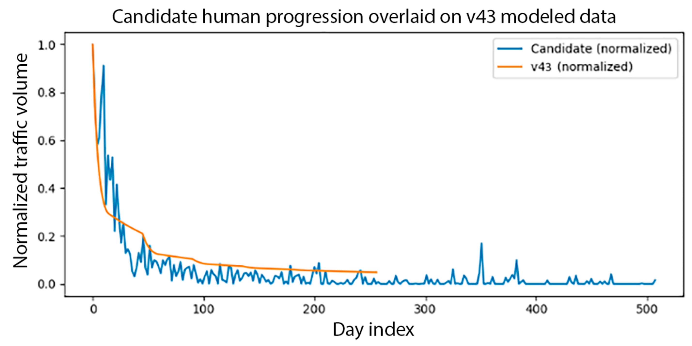
Sample results of the scaling and matching operations are shown in
Figure 3. As discussed, only the decay part of both graphs is used for the matching. Both their initial maximum value had been anchored to each other, and their scaling out to the THRESHOLD day index had been equalized. The MSE value is shown to be 0.008836 for this agent. We selected the 200 user-agents with the lowest MSE values to train our transformer classifier network. MSE value is used as a similarity score for human-likeness, which supports the automated training data selection.
4. Findings
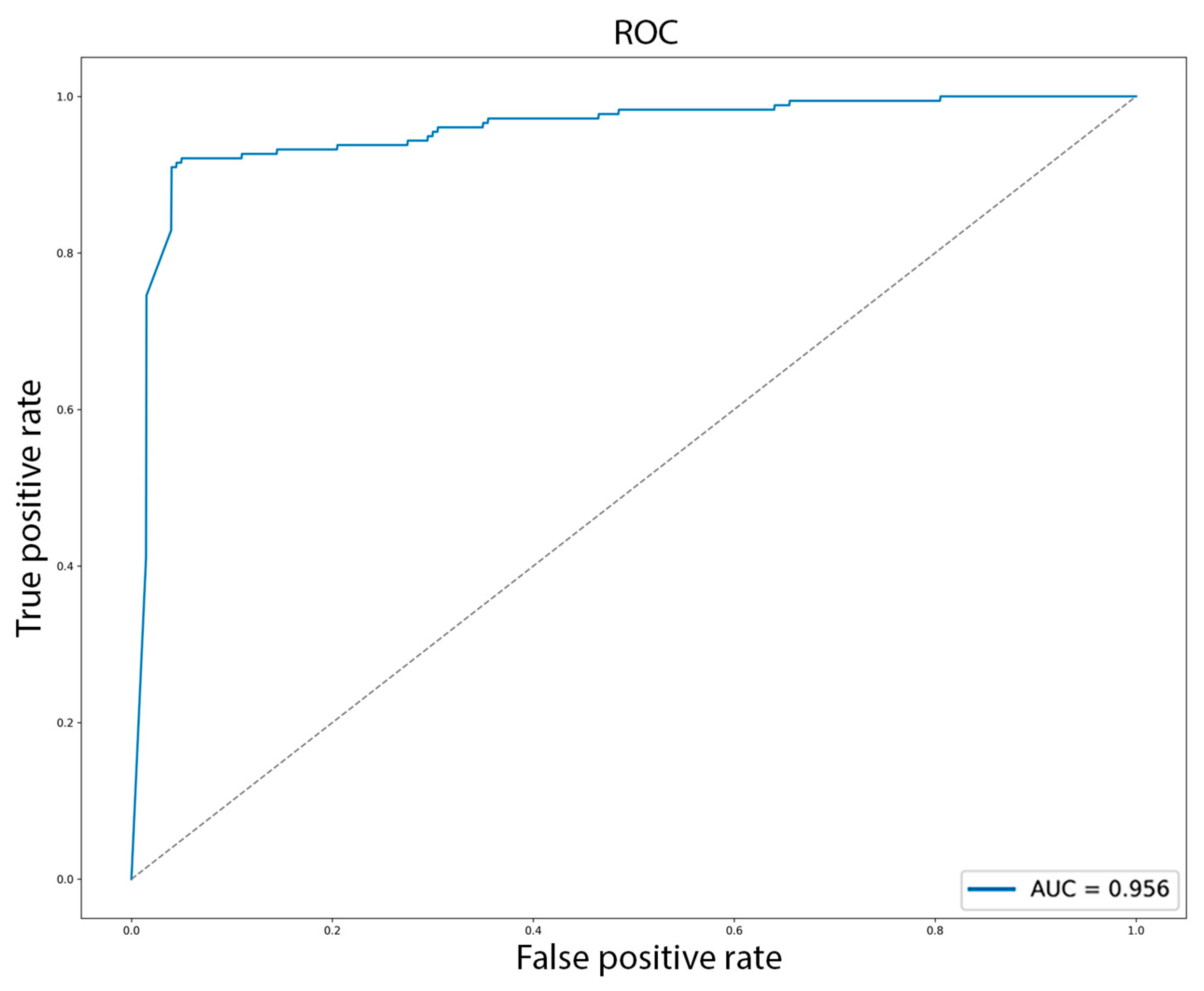
The classification training with a 10% hold-out for verification and a classification threshold of 50% was completed with the following final metrics: Precision: 0.9471, Recall: 0.9096, F1: 0.9280, ROC-AUC: 0.9555. Our method uses the SoftMax output to generate the
, the probability of a hit being robotic for agent
on day index
, so the optimum threshold value does not have to be found. However, optimized for F1, it came out to be 0.234. In this case, the metrics were Precision: 0.9422, Recall: 0.9209, F1: 0.9314, ROC-AUC: 0.9555. The ROC curve is displayed in
Figure 4.
An ROC-AUC close to 1.0 indicates that the model reliably ranks true bots above true human agents across all thresholds. Our score of 0.9555 confirms that the classifier performs well at the chosen F1-optimized cutoff and exhibits strong overall ranking capability, making the bot contamination estimates stable across a wide range of decision boundaries.
To assess the generalization capability of the classifier beyond the training regime, we used the remaining third of our AGWA dataset. It differs from the hold-out sets in that it included all that were not among the best 200 human candidates and were not self-labeled bots. Therefore, these represent agents not used during model training whose contamination level was unknown a priori and could serve as an independent validation corpus.
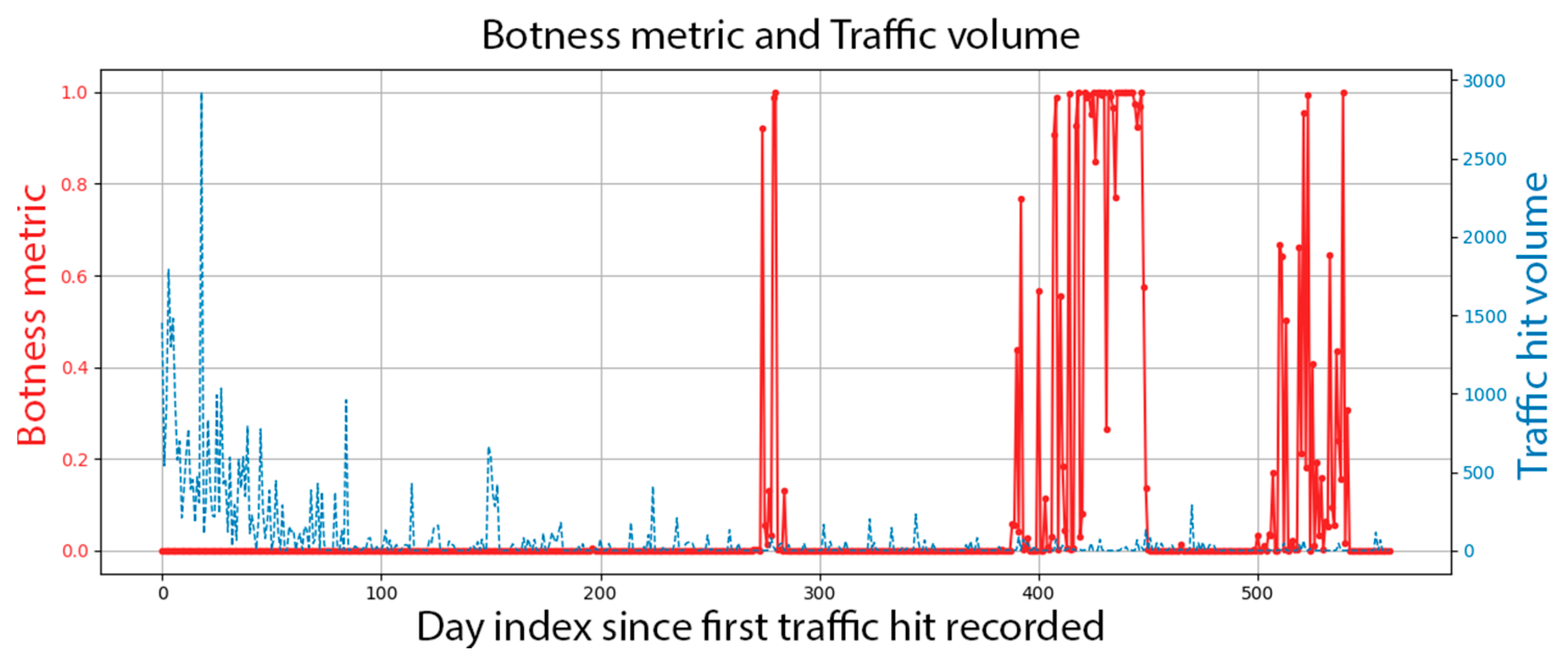
We show the botness evaluation graph of a randomly selected agent in
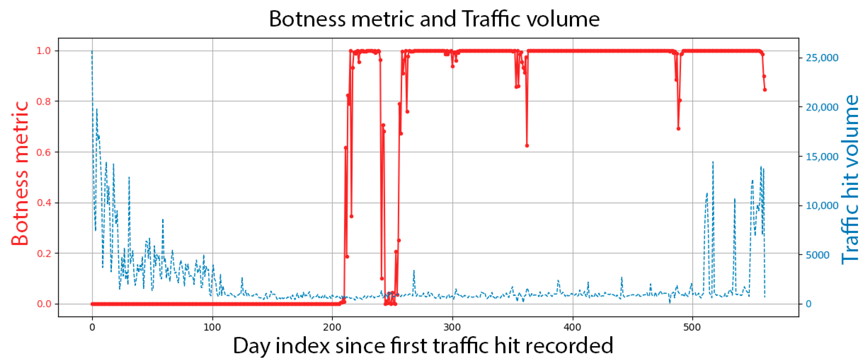
Figure 5; the contamination probability is displayed on the left side as a function of days since the agent string was first observed. The observed daily traffic volume is shown on the right side. Each day’s botness probability is inferred from the feature vectors of the previous 29 days. If we were to evaluate this progression, this is an agent that, when published, had the usage curve of what is expected from a human agency; however, starting after day 200, a bot had hijacked it. The resurgence in traffic volume after day 500 is suspicious, and the inferred botness level indicator agrees.
We also provide two approaches to construct a more rigorous evaluation framework.
4.1. Global Bot-Hit Probability Framework
The inference procedure determines the likelihood of botness for each day. Given that each agent also has its unique traffic volume profile for each day, Equation (8) calculates the global probability for a specific hit to be robotic from agent
.
is thus the predicted global bot probability for agent k for the complete observation windows. This is what we used to find the top- and bottom-ranking agents.
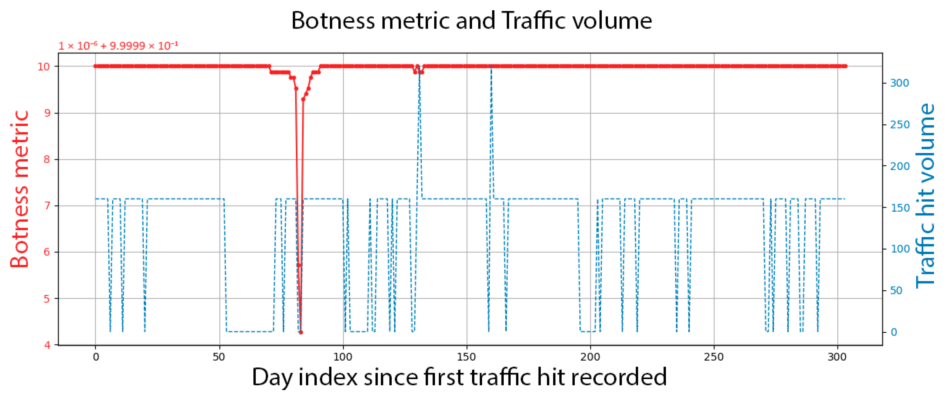
Figure 6 shows the top-ranking agent, which is inferred to be nearly 100% robotic. It shows a constant traffic curve throughout its lifecycle. Some variations are AGWA dataset limitations, where datapoints are missing, or some days were processed together with the previous day’s data, and thus show up as double volume. The agent’s naming error (control characters at the end of the name) further emphasizes the bot’s nature.
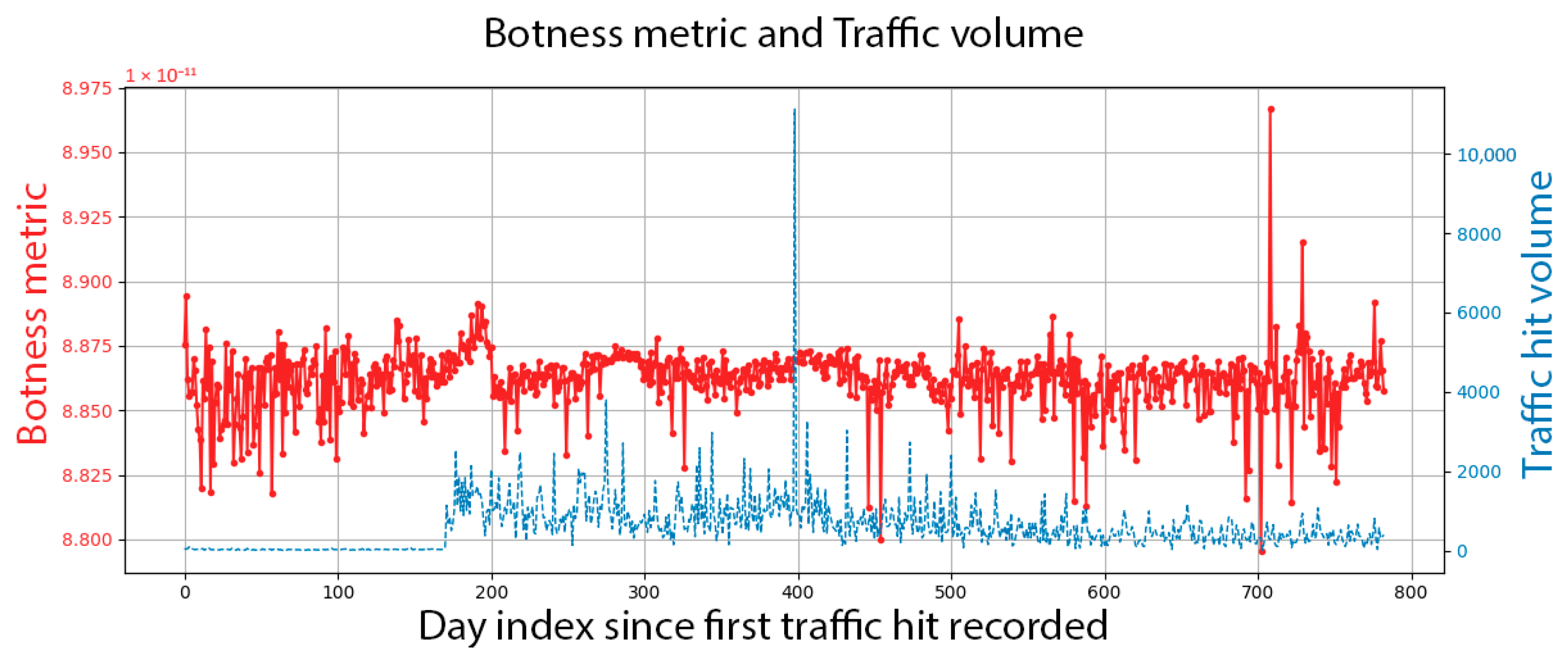
Figure 7 shows the bottom-ranking agent, which is the most likely to be human. This progression is atypical because it was first seen 170 days before its traffic volume began to rise. Even though the traffic is sparse and shows no apparent uptick and decay, the inference did not find it robotic.
4.2. Centroid Distance Analysis
We can use the Transformer encoder’s mean-pooled feature vector for each agent to represent its overall behavioral signature. Separate centroids are computed for each control agent using the same 30-day windowing method used for the training, and a global average for all human sets. We rank all control agents according to their cosine distance from the global human centroid. Cosine distance ranges from 0 (identical patterns) to 1 (maximally different).
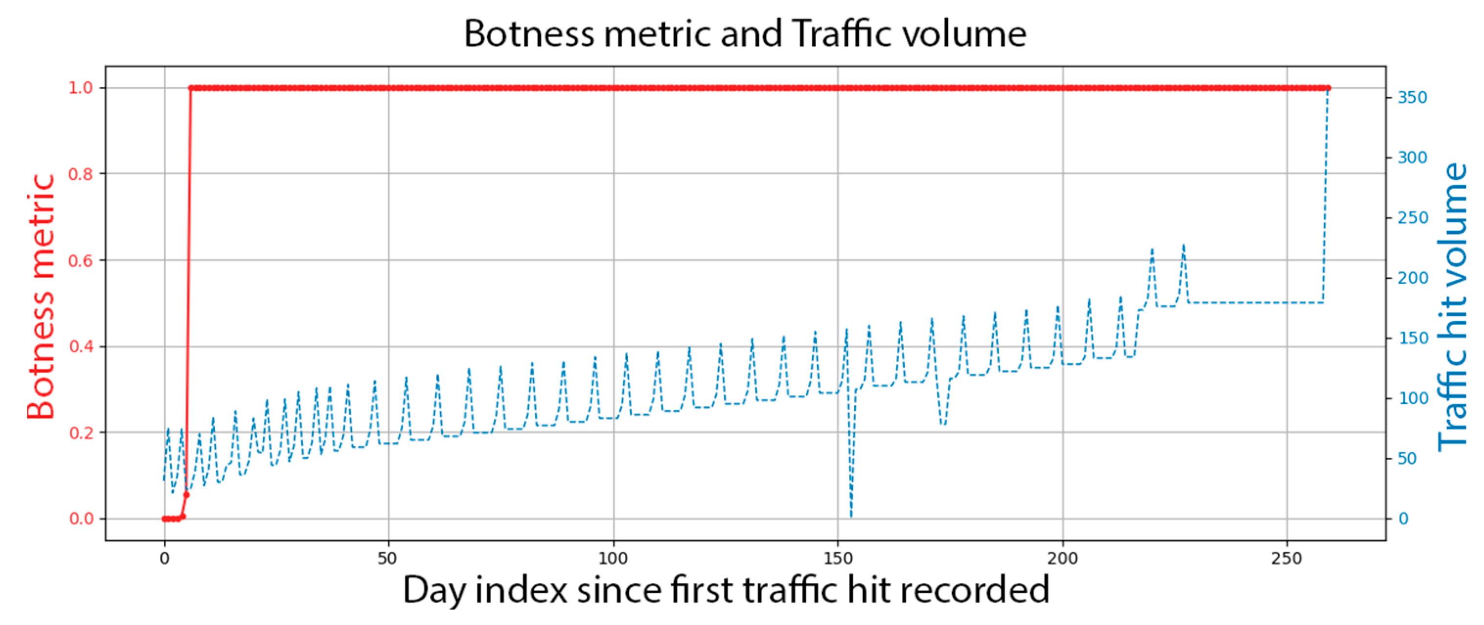
Figure 8 shows the bot agent with the greatest cosine distance from the global human average. The progression clearly shows a periodic element, which is noteworthy since we are not evaluating closeness to bots, but distance from human agency, a pattern with no notion of periodicity. To the expert eye, this is a robotic profile.
Figure 9 shows the most human progression in terms of cosine distance. Notably, unlike the global bot-hit probability, this is inferred to have bot infusion for several months. However, in terms of upramp and decay, it is very close to the training sequences. To the expert eye, this is a human progression, although with relatively little traffic.
5. Conclusions
Our work shows that weighted Transformer-based modeling of user-agent progressions can accurately estimate bot contamination, even with noisy or incomplete data. Although we used days as our units of investigation, the models can be updated based on new incoming data with greater frequency, although the hourly processing of new logs is a sweet spot.
Once service providers can pre-filter high-likelihood agents, they can be processed using the industry standard UI fingerprinting or biometrics-assisted methods. The rest can be served unimpeded. Depending on the service load, the cutoff for active bot testing can be adjusted dynamically to ensure that the system can handle the legitimate demand at optimal latency for human visitors. This can ultimately reduce operational costs and improve the service reliability of the existing infrastructure.
More broadly, we see contamination scoring as a practical tool for more innovative resource management. Traffic trust levels can be integrated into load balancing, firewall rules, and service pricing strategies, helping operators prioritize real users, minimize waste, and plan infrastructure more efficiently.
6. Limitations and Future Work
We employed several heuristic steps to separate human and robotic traffic in the AGWA dataset. The self-tagging for bot agents is considered reliable, given the large number of samples and the limited incentive for humans to misrepresent themselves as bots. However, the identification of human samples while model-based still relied on real feature vectors from observed progressions. This raises the possibility that some training samples contained residual bot contamination, which could bias the model toward underestimating the actual botness level. A factor that may require corrections in downstream processing.
Due to privacy concerns, third-party datasets in raw Apache log format are difficult to obtain. When such datasets are available, they typically only provide binary labels (bot, non-bot) rather than continuous contamination percentages across observation windows. However, we are working with service providers and IP blacklist providers to generate a self-tagging database for bot traffic.
In parallel, we are developing an independent tagging approach based on honeypot data, which monitors access attempts to files commonly associated with penetration testing and distributed denial-of-service (DDoS) activity. These complementary methods aim to improve both the training and verification accuracy.
