Abstract
Pricing catastrophe (CAT) bonds in incomplete markets poses persistent challenges, particularly in converting risk from the real-world measure to the pricing measure. The commonly used Wang transform focuses on distorting the loss severity distribution, which may underestimate catastrophe risk. This paper proposes a new distortion operator based on the Esscher transform that distorts the aggregate loss distribution rather than focusing solely on the severity or frequency components. The proposed approach provides more comprehensive risk adjustment, making it well-suited for the distributional characteristics of catastrophic loss indicators. Its applicability is demonstrated via an application to Chinese earthquake data. Monte Carlo simulation was used to compare pricing results via the distortion of different components. By reformulating the proposed distortion method into the form of a distortion operator and comparing it with the Wang transform, this paper demonstrates that the proposed approach offers significantly enhanced analytical tractability for complex distributions. It enables a more transparent analysis of the transformed distribution and its implications for bond pricing mechanisms.
MSC:
62P05; 62P20; 91G20; 91G70
1. Introduction
In the context of global climate change, the frequency of catastrophic events and their resulting economic losses has been steadily increasing [1]. These events have profound and intricate impacts on economies and societies. The advancement of economic globalization has expanded the reach of these disasters beyond specific regions, affecting global trade and supply chain networks and causing widespread economic instability [2]. Consequently, the importance of managing catastrophe risks has become increasingly crucial to maintaining global economic stability. Traditional insurance markets face significant limitations in addressing catastrophe risks. Firstly, their underwriting capacity is constrained by the growing scale and frequency of catastrophic events, making it challenging to meet the rising demand for risk coverage. Secondly, catastrophe risks often entail high premium loading due to their inherent uncertainty and complexity. Traditional insurers typically include substantial risk premiums in their pricing models, resulting in excessively high insurance costs for many individuals and businesses [3]. Therefore, tapping into external capital markets has become a vital alternative to fulfill the financial requirements for compensating catastrophe risk losses.
Insurance-linked securities (ILSs) provide an important risk transfer and capital-raising avenue for insurers and reinsurers, effectively alleviating the capital strain imposed by catastrophic risks through the infusion of external capital [4]. Over the past two decades, the catastrophe derivatives market has experienced rapid growth, with CAT bonds emerging as the most successful instrument for hedging catastrophe risk and playing an essential role in asset allocation and risk management [5,6]. Investors are attracted to CAT bonds primarily due to two aspects. First, as a “zero-beta” asset, catastrophe risk exhibits a low correlation with traditional financial market risks, providing significant portfolio diversification benefits to investors [7,8]. Second, CAT bonds typically offer relatively higher yields, with expected returns generally exceeding the average levels observed in financial markets [9].
The CAT bond pricing model, by precisely quantifying the dynamic relationship between risk and the capital markets, has served as a core financial tool for the effective transfer and diversification of extreme catastrophe risks. Given that catastrophe risks cannot be fully replicated by traditional financial instruments such as bonds or equities, CAT bond pricing must be conducted within an incomplete market framework. Commonly adopted pricing methodologies include the probability transform pricing approach, the equilibrium pricing approach, and the utility indifference pricing approach.
The probability transform pricing approach, due to its theoretical simplicity and computational tractability, has been widely applied in CAT bond pricing. This method adjusts the loss distribution or the risk measure to reflect market risk preferences, thereby deriving risk-adjusted prices. It plays a critical role in determining an appropriate risk loading, particularly when accounting for subjective risk preferences, and is consistent with the utility-based framework in financial theory [10]. Venter was among the first to advocate for pricing financial products based on risk-adjusted probability distributions [11]. The Wang transform has been widely regarded as a foundational technique in this context [12,13,14]. By introducing a nonlinear adjustment to the cumulative distribution function and incorporating a risk aversion parameter, the Wang transform unifies the pricing principles across insurance and finance, encompassing pricing models such as the standard deviation principle, the Capital Asset Pricing Model (CAPM), and the Black–Scholes option pricing framework. However, catastrophe risks are often characterized by heavy-tailed and skewed distributions, while the classical Wang transform is derived under the assumption of normality, limiting its applicability to such risks. To overcome this limitation, [15] proposed a class of distortion operators based on the Normal Inverse Gaussian distribution, which allows for flexible adjustment of tail distortion and demonstrates effectiveness in handling heavy-tailed and skewed distributions. The authors of [16] further introduced a general framework for constructing distortion operators that can flexibly adapt to various underlying distributions, accommodating diverse market conditions and risk characteristics. This framework remains consistent with various pricing principles in finance and insurance, such as the Esscher transform, the proportional hazards (PH) transform, and the size-biased transform [12,15,17,18]. Overall, the probability transform pricing approach not only parametrically captures risk preferences but also demonstrates strong robustness under complex distribution assumptions, becoming one of the primary methods for pricing CAT bonds.
While the equilibrium pricing approach and the utility indifference pricing approach are theoretically relatively comprehensive, their practical application is constrained by the availability of market data and their underlying assumptions. For instance, the equilibrium pricing approach determines the price of CAT bonds based on the market supply and demand dynamics [19,20], necessitating explicit assumptions about the risk preferences of market participants, which are challenging to validate in CAT bond transactions. The utility indifference pricing approach [21,22] requires the precise specification of investors’ utility functions. The calculation process is complex and highly sensitive to the accuracy of market environment assumptions. It requires comprehensive consideration of market conditions, risk characteristics, and expected returns influencing pricing decisions. In contrast, the probability transform pricing approach offers a more straightforward computational framework, requiring only knowledge of market risk preferences to derive prices, thereby offering notable advantages in both theoretical modeling and empirical application.
One of the principal challenges in catastrophe risk management arises from the dual stochastic nature of catastrophic events, namely, the randomness in event frequency and loss severity. Consequently, the aggregate loss distribution is widely used in both actuarial practice and academic modeling, since it naturally integrates frequency and severity components under a single probabilistic object. For the frequency component, the Poisson process remains the mainstream modeling tool. For severity, heavy-tailed distributions such as the Pareto, Gamma, and Weibull distributions are commonly employed [23,24]. Additionally, clustering effects of catastrophes can be characterized using Hawkes processes and compound Poisson processes [25,26,27]. Probability distortion techniques can incorporate risk preferences into Insurance-Linked Securities (ILSs) and catastrophe (CAT) bonds pricing models, and prior research has largely concentrated on applying distortions to either the loss severity distribution or the loss frequency distribution. Among these, the Wang transform remains the most widely adopted tool for adjusting severity distributions, and it has been extensively implemented in both theoretical and applied studies [28,29,30,31]. Moreover, for binary payoff structures, distortion of the frequency component through the Wang transform has also been explored, as discussed in [28]. Alongside this strand of research, a growing body of work has shifted attention toward the aggregate loss distribution. The authors of [32,33] employ Bayesian inference and simulation-based methods to capture uncertainty in aggregate claims processes, which underscore the importance of aggregate modeling but do not rely on distortion-based valuation principles.
While distortion techniques are well-established for adjusting marginal frequency or severity distributions and aggregate loss modeling has advanced through other means, a critical gap emerges at the intersection of these fields. The current literature, particularly from 2019 to 2025, shows a clear preference for either marginal distortions (e.g., Wang transform) or non-distortion-based aggregate models (e.g., Bayesian frameworks). Consequently, the concept of directly distorting the aggregate loss distribution itself as a foundation for CAT bond pricing remains a significant, unaddressed opportunity. Our research confronts this gap directly by introducing a novel framework that embeds distortion operators at the aggregate loss level. This integration of aggregate modeling with distortion-based valuation provides a more holistic risk adjustment mechanism, enhancing the sensitivity and practicality of CAT bond pricing.
The primary contributions of this paper are as follows: First, within the product pricing measure framework, we propose a novel CAT bond pricing approach based on direct distortion of the aggregate loss distribution. This method unifies and extends conventional approaches that typically address frequency and severity distributions in isolation. Second, using the Esscher transform, we theoretically demonstrate that distorting the aggregate loss distribution can be explicitly decomposed into simultaneous adjustments to both the frequency and severity distribution parameters. This decomposition ensures theoretical coherence while preserving analytical tractability. Third, empirical analysis of Chinese earthquake CAT bonds confirms the framework’s high efficiency in risk adjustment. Specifically, for a given market-consistent pricing target, the method requires only minimal parameter adjustments. This indicates its ability to retain the original risk distribution structure to the greatest extent while achieving the target risk premium, thereby avoiding excessive distortion. Fourth, Monte Carlo simulations comparing the proposed aggregate loss distortion approach with the widely used Wang transform show that the proposed method offers significantly enhanced analytical tractability for aggregate distributions. This leads to more transparent interpretation of the transformed distribution and clearer implications for bond pricing.
The rest of this paper is organized as follows: In Section 2, we present the pricing framework for CAT bonds, including the product pricing measure, measure transform, and detailed pricing formulas. Section 3 conducts an empirical analysis using Chinese earthquake data. In Section 4, we compare aggregate loss distortion with other distortion methods and examine the sensitivity of bond prices to key parameters. Section 5 concludes the paper.
2. CAT Bond Pricing Framework
2.1. Product Pricing Measure
In CAT bond pricing, it is essential to account for two primary sources of risk: catastrophe risk and financial market risk. The former dictates the likelihood and extent of payouts throughout the bond’s maturity, while the latter impacts coupon payments and final bond pricing by discounting potential outflows. The assumption of independence between catastrophe risk and financial market risk in catastrophe bond pricing is a well-founded premise. From a theoretical standpoint, catastrophe risk originates from localized, physical events such as earthquakes or hurricanes, whose occurrence mechanisms are fundamentally disconnected from the macroeconomic and systemic factors driving financial market risk. This dichotomy in risk generators provides a theoretical basis for treating them as independent. Empirically, numerous studies have documented a historically low correlation between catastrophe losses and financial market performance [7,8], particularly when the catastrophe risk is region-specific, while the financial variables are global in nature, which further supports the independence assumption from a statistical perspective. Although this assumption may not hold during periods of extreme systemic crisis where contagion effects could amplify correlations, it remains a reasonable and robust baseline approximation for typical catastrophe bond structures under ordinary market conditions.
The physical probability space of catastrophe risk and financial market risk are defined as and . Since there are almost no correlations between these risks, we can assume that the two spaces are independent of each other, leading to the construction of a product space , where , , , . For more discussion of product spaces, see [19,28].
In CAT bond pricing, two probability spaces necessitate different pricing approaches. For catastrophe risks, since it is difficult to achieve perfect replication, an incomplete market pricing approach is adopted. Under the probability transform pricing framework, the original risk in the real-world probability measure undergoes a probability distribution distortion to yield a new probability measure . This transformation incorporates a distortion operator to reflect the investors’ attitude toward CAT risk. It enables the nonlinear weighting of losses across different magnitudes, allowing for the flexible modeling of investor risk preferences and sensitivity to tail risk. In contrast, financial market risk is priced using the no-arbitrage principle, where interest rate risk is evaluated under the risk-neutral measure .
Given the assumption of independence between the two probability spaces, probability measure transformation can be applied separately. Let the probability measures obtained by distorting and be denoted by and , respectively. The final price of the CAT bond is then calculated based on the product measure , incorporating the distributions of both catastrophe risk and financial market risk.
2.2. Pricing Formula
Assuming that the trigger of catastrophe risk is , which is a stochastic process defined on , this can be designed as
where denotes the counting process that records the occurrence times of catastrophe events. represents the magnitude of each event, such as earthquake magnitude or the associated economic loss. We assume that the CAT bond is issued at time 0 and matures at time T. At any time , the remaining principal of the bond depends on the value of the trigger variable over the interval . Let be a non-increasing, right-continuous function representing the proportion of the remaining principal. At the initial time, the remaining principal proportion is 100%, i.e., . If the bond has a face value of K, then the remaining principal at time t can be expressed as .
Without loss of generality, we assume that coupon payments are made at the end of each quarter. Let , so that coupon payment times are for . Each coupon payment is proportional to the principal remaining at the time of the previous coupon payment and fluctuates with the three-month LIBOR. If the fixed coupon rate is R and the LIBOR is , the coupon amount paid at each time point is given by
The bond will terminate upon the earlier of: (i) the full loss of principal due to the occurrence of a series of catastrophic events, or (ii) the expiration of the bond’s term. We denote the time of principal wipeout by . If the principal is not exhausted by maturity (), then coupon payments continue as scheduled until maturity, and the remaining principal is repaid at the maturity date. If the principal is exhausted within the bond term (), the last coupon is paid when the principal is exhausted, and the bond terminates.
If time is not a coupon payment date, then the last coupon payment at time is , where is defined as follows:
where denotes the floor function.
CAT bonds are issued in the international market, so we use 3-month U.S. Treasury yield as the market risk-free interest rate.
Based on the above settings, the price of CAT bond at time t can be expressed as [28]
In the above formula, denotes the expectation under conditional on the available information up to time t. D is the discount factor, where .
Pricing Formula (4) includes both catastrophe risk and financial market risk, thus avoiding the time inconsistency problem in bond pricing. Below, Section 2.3 and Section 2.4 discuss how to transfer catastrophe risk and financial market risk, respectively, from the measure to the measure.
2.3. Esscher Transform of Aggregate Loss Distribution
CAT bonds require the modeling of catastrophe risk within a specified time frame. To this end, two independent stochastic processes are typically employed: one to characterize the frequency of events and the other to represent the severity, i.e., the magnitude of each catastrophe event. The aggregate loss distribution captures the joint effect of frequency and severity, providing a comprehensive characterization of the potential loss magnitude.
Let X be a continuous random variable defined on , representing the catastrophe risk loss occurring from time 0 to T. Then X can be expressed as
The random variable N follows a discrete distribution (e.g., Poisson distribution) with the following probabilities:
The random variables are assumed to follow a continuous distribution defined on the non-negative real axis and are independent of N. We assume that are i.i.d.; then, the distribution of the aggregate loss X can be expressed as
where
To compensate bond investors for bearing catastrophe risk, it is essential to incorporate an appropriate risk premium into pricing. Under the product pricing measure framework, this is achieved through a probability distortion approach that reflects investor risk preferences. The Esscher transform has been widely used in risk-neutral pricing, option valuation, and premium calculation. The following section explores how to apply the Esscher transform to the distribution of aggregate loss.
Theorem 1.
By applying the Esscher transform, the distribution of aggregate loss X can be shifted from the original probability space to the transformed probability space . The cumulative distribution function of X after the Esscher transform is
For positive integer n, it holds that
is the probability density function of after the Esscher transform with parameter h.
Proof.
Let represent the total losses from n catastrophic events. Its cumulative distribution function under is , and its probability density function is . Let .
The Radon–Nikodym derivative of the probability measure defined by the Esscher transform with respect to the probability measure is
When , the larger the value of the parameter h, the thicker the tail of the distorted density function. Based on the characteristics of catastrophic events, this article only considers the case of . Therefore, after the Esscher transform, the cumulative distribution function of X on the measure can be expressed as
□
We select the Esscher transform as the distortion tool due to its excellent mathematical properties and analytical tractability, particularly for distributions within the exponential family. It is important to note that the application of this transform is predicated on the existence of the moment-generating function of the risk distribution in the neighborhood of the transform parameter h. Consequently, the direct scope of our framework applies to loss distributions for which the moment-generating function is well-defined, a condition met by the vast majority of distributions commonly used in actuarial and financial practice.
Proposition 1
(Uniqueness of the Decomposition for Theorem 1). In Theorem 1, the frequency–severity decomposition induced by the Esscher transform is unique.
Proof.
Suppose that under the probability measure , the distribution of X follows a frequency–severity compound distribution structure. We define a new frequency distribution , where . We define a new cumulative distribution function .
(1) Proof of (9).
can be expressed as the expectation of an indicator function:
According to (12),
By the law of total expectation, we have
(2) Proof of (10).
For any and , we have
We have proven that . We compute the above equation’s numerator:
By the law of total expectation, we have
By substituting , after simplification, we obtain (assuming )
We write this in integral form:
The above formula is the same as (10) in Theorem 1. This concludes the proof of .
Since any decomposition that satisfies this compound structure must be of this form, it follows that the decomposition is unique. □
Based on (9), under the Esscher transform of the aggregate loss distribution, the distortion of the frequency distribution is not independent but is instead determined by the distortion of the severity distribution. Notably, this adjustment mechanism for the frequency distribution has the property of point-wise adjustment, thus exhibiting broad distributional compatibility. Specifically, this adjustment method is not only applicable to standard discrete distributions but can also effectively handle types of discrete distributions with complex structures, such as zero-modified and zero-inflated distributions.
From Theorem 1, when the severity distribution has infinite divisibility, can maintain the same distributional form as , and the result of the frequency and severity distribution distortions has an analytical solution. For example, the Exponential, Gamma, Normal, and Inverse Gaussian distributions all have the infinite divisibility. In what follows, we provide a detailed explanation using the case where the severity distribution follows a Gamma distribution as an example.
Corollary 1.
When the loss severity follows a Gamma distribution, the Esscher transform of the aggregate total loss can be decomposed into the result of separately applying distortion transforms to the severity random variables for each risk event and to the frequency random variable N.
Proof.
The result of the distortion for the frequency distribution is given in (9). In what follows, we only prove the distortion transform for the severity distribution.
Suppose that are i.i.d. and follow a Gamma distribution, denoted by , with the density function . We now prove that .
By applying the Esscher transform to the distributions of , the resulting probability density function under the measure can be expressed as
Under the measure, . In the above Esscher transform, the range of the parameter h is .
Let ; by the infinite divisibility of the Gamma distribution, . Similarly, under the measure, , and we let its probability density function under the measure be .
Below, we prove that using the moment-generating function.
The moment-generating function of is
The moment-generating function of is
So,
From Theorem 1, when the loss severities are i.i.d. and follow a Gamma distribution, applying an Esscher transform with parameter h to the aggregate loss distribution not only adjusts the distribution of individual losses to that resulting from an Esscher transform with parameter h but also indirectly affects the statistical properties of the loss frequency.
Furthermore, using the properties of the Gamma distribution, the distortion transform of the frequency distribution can be simplified to
It can be seen that the frequency distribution after the distortion transform has a heavier tail. □
Corollary 2.
When the number of losses N follows a Poisson distribution with parameter λ and the loss severity follows a Gamma distribution with parameters , applying an Esscher transform with parameter h to the aggregate loss is equivalent to adjusting the mean parameter of the Poisson distribution from λ to and to adjusting the rate parameter of the Gamma distribution from θ to .
Proof.
Corollary 1 has established the result for the adjustment of the loss severity distribution. We now examine the adjusted distribution for the number of losses. For the denominator of (24), the calculation is as follows:
Therefore, the distortion transform of the frequency distribution can be further simplified to
Thus, applying an Esscher transform with parameter h to the aggregate loss is equivalent to adjusting the mean parameter of the Poisson distribution for the number of losses N from to and to adjusting the rate parameter of the Gamma distribution for the loss severity from to . □
Corollary 2 decomposes the distortion transform of the aggregate loss distribution into two parts: one is the distortion transform of the frequency distribution, and the other is the distortion transform of the severity distribution. In this case, the distorted loss frequency and loss severity distributions can be calculated directly, thereby simplifying the distortion transform of the aggregate loss distribution.
2.4. The Risk-Neutral Measure Transformation of Market Interest Rates
In CAT bond pricing, the discount factor should use the risk-free rate that matches the frequency of coupon payments. Here we use the 3-month U.S. Treasury yield.
According to (4), the pricing formula for CAT bonds involves the expectations of two discount factors. The first is the expectation of a discount factor that includes two interest rate components, the LIBOR and the risk-free rate, given by . The second is the expectation of a discount factor that includes only the risk-free rate, denoted by . We model the floating rate LIBOR and the risk-free rate by using a double Vasicek model. The choice of the Vasicek model is motivated by several considerations. First, it accommodates negative interest rates, as observed in historical U.S. Treasury yields, ensuring consistency with market conditions. Second, it provides closed-form solutions for discount factors in CAT bond pricing (see (26) and (27)), avoiding the computational burden of nested simulations. Third, its mean-reversion property and ease of calibration enhance transparency and numerical stability relative to alternatives such as the CIR model. Overall, the Vasicek model offers an efficient and tractable framework for interest rate modeling in catastrophe bond pricing.
Let the risk-free rate be denoted by r and the floating rate by l. The double Vasicek model for the interest rates can then be expressed as
where and represent the speed of the long-term mean reversion of interest rate. and represent the long-term mean level of the interest rate. and represent the volatility of the interest rate, and and represent standard Brownian motion.
In the pricing formula for CAT bonds, and under the risk-neutral measure can be computed as follows [34]:
where
3. Empirical Analysis
Similar to traditional indemnity-based catastrophe insurance, CAT bonds with indemnity triggers face inherent challenges, such as lengthy settlement periods and the potential for moral hazard. In contrast, index-based CAT bonds determine payouts based on objective and quantifiable physical parameters of actual disaster events. This structure effectively mitigates moral hazard and removes the uncertainty associated with manual loss assessment, thereby enabling a more rapid response in the aftermath of a catastrophe. Empirical studies have shown that index-based CAT bonds are generally priced lower and are thus more consistent with market demand [7,35]. In light of these advantages, this section develops a pricing model for index-based earthquake CAT bonds and explores its practical implementation.
For the empirical analysis, we collect data on all earthquake disaster events in mainland China (excluding Hong Kong, Macao, and Taiwan) from 1949 to 2019, excluding events with epicenters at sea or outside the national borders. The dataset used in this study was obtained from the China Earthquake Networks Center (http://data.earthquake.cn (accessed on 1 June 2023)). All selected earthquakes have magnitudes of 4.0 or greater. Given the generally positive correlation between earthquake magnitude and economic losses, earthquake magnitude is adopted as the trigger variable in the design of the earthquake CAT bond.
3.1. Fitting Earthquake Magnitude Distribution
In catastrophe risk modeling, the frequency–severity framework is widely adopted. The frequency of events is typically modeled using a Poisson process [22,28,35,36], while the severity is characterized using heavy-tailed or extreme value distributions [28,37].
For earthquake magnitude data in mainland China, multiple continuous distributions were fitted and compared. Among them, the Gamma distribution exhibited the best fit, with the Q–Q plot aligning closely to a straight line. Given that earthquakes of magnitude 4.0 and above can be treated as left-truncated data, a left-truncated Gamma distribution was employed. Under this assumption, the probability density function of the earthquake magnitude is expressed as
The parameters estimated using the maximum likelihood method are , , and . The diagnostic plots are presented in Figure 1, which shows that (29) has a good fit.
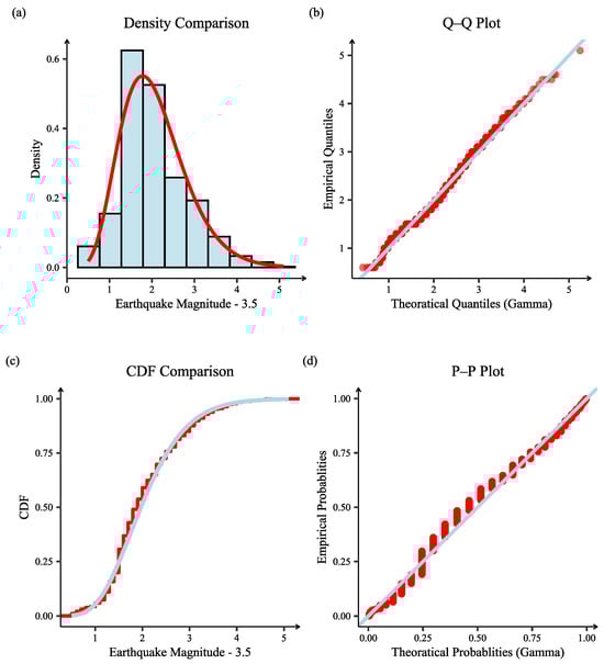
Figure 1.
Diagnostic plots for the fitted truncated Gamma distribution to the magnitude of earthquakes above 4.0 in China (1970–2019). (a) Histogram of the sample data and the probability density function (PDF) of the fitted distribution (red line); (b) Quantile–Quantile (Q–Q) plot, where points closely following the diagonal line indicate a good fit between the empirical and theoretical quantiles; (c) Comparison of the empirical cumulative distribution function (ECDF) from the data (red line) with the theoretical cumulative distribution function (CDF) of the fitted distribution (blue line); (d) Probability–Probability (P–P) plot, where the alignment to the diagonal suggests the model adequately captures the data distribution.
To validate the temporal stability of the magnitude distribution, we performed parameter stability and out-of-sample forecasting tests within a rolling-window backtesting framework.
For the parameter stability test, we initiate with a 40-year data window. Equation (29) is then refit annually as the window rolls forward one year at a time. Figure 2 plots the evolution of the parameter estimations over this period. The Gamma distribution parameters, and , exhibit remarkable stability throughout the sample period. This provides strong justification for using the full-sample data for a single, static model fitting in our main analysis.
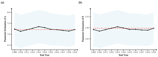
Figure 2.
Parameter stability test for the truncated Gamma distribution. (a) Rolling estimates for the parameter ; (b) Rolling estimates for the parameter . The black point in each plot represents the point estimate. The blue-shaded regions represent their 95% confidence intervals, while the red dashed lines indicate the values estimated from the full dataset.
For the out-of-sample forecasting test, we use the data up to the end of each window to fit the distribution. We then employ the Kolmogorov–Smirnov test to assess if this fitted distribution adequately describes the data of the subsequent year. Figure 3 displays the resulting p-values from these KS tests. All of p-values lie above the 0.05 significance threshold (the red line), meaning that we fail to reject the null hypothesis that the next year’s data are drawn from the distribution fitted on historical data (p-value > 0.05). This indicates that the earthquake magnitude distribution built on historical data has strong predictive and descriptive power for the following year.
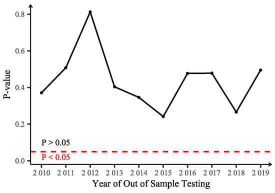
Figure 3.
Out-of-sample forecasting test of parameter stationarity. The black dots represent the p-value for each annual test. The horizontal red dashed line indicates the 5% significance level.
The frequency of earthquake occurrences is modeled using a Poisson process. A histogram of earthquakes with magnitude above 4.0 between 1949 and 2019 reveals relatively low frequencies before 1970, possibly due to data incompleteness, which can be seen in Figure 4a. Therefore, we estimate the Poisson parameter using data from 1970 to 2019, yielding . A Kolmogorov–Smirnov test of exponential inter-arrival times yields a p-value of 0.8607, failing to reject the null hypothesis that earthquake arrivals follow a Poisson process. The diagnostic plots are presented in Figure 4b,c, which show a good fit.
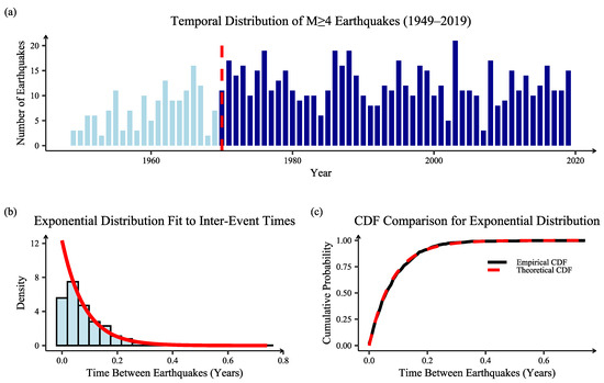
Figure 4.
Goodness-of-fit analysis for modeling annual earthquake frequency as a Poisson process (1970–2019). (a) Bar chart of the number of seismic events recorded per year, illustrating the annual frequency distribution, and the red dashed line indicates the year 1970; (b) Histogram of the inter-event times (time between two consecutive earthquakes), and the probability density function (PDF) of the fitted exponential distribution (red line), where the alignment suggests that inter-event times are exponentially distributed; (c) Comparison of the empirical cumulative distribution function (ECDF) of the inter-event times with the theoretical CDF of the fitted exponential distribution, providing a diagnostic check for the quality of the fit.
3.2. Design of Indemnity Mechanism
In this study, earthquake magnitude is selected as the trigger variable, which is a result of a comprehensive consideration of multiple factors, including the design principles of a parameterized trigger mechanism, data reliability, model manageability, and industry practices. Compared with physical intensity indices such as peak ground acceleration (PGA), peak ground velocity (PGV), or the Modified Mercalli Intensity (MMI), earthquake magnitude is an absolute physical measurement with a high degree of standardization and comparability. This significantly reduces model risk and complexity caused by uneven station distribution, interpolation method differences, and regional heterogeneity. From the perspective of securitization product design, using earthquake magnitude as the core trigger parameter aligns with the core requirements of insurance-linked securities for transparency, execution efficiency, and moral hazard management. Once an earthquake event exceeds a preset threshold, compensation is automatically triggered, eliminating the need for cumbersome and potentially contentious actual loss assessment processes, significantly improving fund operation efficiency and contract enforceability.
Undeniably, there is a nonlinear mapping between earthquake magnitude and ultimate economic losses due to factors such as focal depth, local geological conditions, and population and economic exposure, which may introduce basis risk. This study introduces a multi-layered triggering mechanism into the trigger structure design to mitigate the loss bias caused by the nonlinear relationship between earthquake magnitude and economic losses. The multi-layered payout structure defines that when the earthquake magnitude reaches the 98th, 99th, 99.5th, and 99.9th percentiles, the catastrophe bond triggers payouts of 25%, 50%, 75%, and 100% of the principal, respectively.
We assume that the bond is issued at time and matures at time T. The depletion of the principal over time, denoted by , can be defined as
Here, denotes the number of earthquakes that occurred within the time interval , and represents the magnitude of the n-th earthquake. The corresponding remaining principal ratio function is defined as
3.3. Parameter Estimation for the Interest Rate Model
We assume that a one-year Chinese earthquake CAT bond was issued on 2 January 2020. To estimate the parameters of the interest rate model, we use historical data on U.S. 3-month Treasury yields and 3-month LIBORs from 4 January 2006 to 31 December 2019 (the LIBOR is now gradually being replaced by alternative rates such as the SOFR). The risk-free rate and the LIBOR are assumed to follow the double Vasicek model under the real-world probability measure . Model parameters are estimated using the maximum likelihood method, with results reported in Table 1, where and represent the speed of the long-term mean reversion of interest rate, and represent the long-term mean level of the interest rate under measure, and and represent the volatility of the interest rate. Here, and represent the values of the risk-free rate and the LIBOR, respectively, on 2 January 2020.

Table 1.
Parameter estimation of the double Vasicek model under the measure.
To translate the parameter estimation under the real-world measure into the risk-neutral measure , it is necessary to estimate the market price of interest rate risk, denoted by . We use the U.S. Treasury yield with maturities ranging from 6 months to 30 years on 2 January 2020 as the yields of zero-coupon bonds under . According to the Vasicek model, the price of a zero-coupon bond maturing at time T is given by
where
is the long-term mean under the risk-neutral measure .
The theoretical yield of the zero-coupon bond with a term of T can be calculated as
Our objective is to calibrate the theoretical Y(0, T) to the observed market yield under over all maturities. We begin by substituting the Vasicek model estimation parameters of the risk-free rate under in Table 1 into (32). The theoretical yield with as the parameter can be calculated for different maturities. Meanwhile, the yields of U.S. Treasury bonds with maturities from 6 months to 30 years are used as the market yield. By minimizing the sum of squared errors (SSE) between the theoretical model yield and the market yield over all maturities, the optimal can be obtained through a numerical optimization algorithm. The result is 0.0354. The corresponding minimum SSE is 2.34 × 10⁻⁵. Thus, the estimation parameters for the two interest rate processes under the risk-neutral measure are presented in Table 2. By substituting the risk-neutral parameters from Table 2 into (26)–(28), we obtain the discount factors required in the CAT bond pricing formula.
Table 2.
Parameter estimation of the double Vasicek model under the measure.
3.4. Simulation of Bond Price
To assess earthquake catastrophe risk, we conduct Monte Carlo simulations of catastrophe event paths over a 360-day horizon, using 100,000 simulated scenarios. Within the product measure pricing framework, interest rate risk is adjusted to the risk-neutral measure, and earthquake risk is distorted via a change in measure. Subsequently, future cash flows over the one-year bond term are discounted to the issuance date (2 January 2020) using the risk-free rate. For each simulation path, the time of principal exhaustion is determined first, and then the bond price at time zero is calculated according to the bond pricing formula.
To enhance simulation efficiency, particularly for claims driven by low-frequency, high-severity earthquake events, importance sampling is applied to the earthquake magnitudes. This technique alters the sampling process by introducing a proposal distribution and importance weights. By doing so, it increases the sampling frequency of critical rare events, thereby improving the statistical efficiency of the simulation.
Reflecting the piece-wise structure of the bond’s payout function, the magnitude domain is partitioned into several disjoint strata. This design aligns the sampling strata directly with the bond’s payout tiers, which mitigates spurious sampling variance. So we use stratified importance sampling for earthquake magnitude. In contrast to conventional importance sampling that uses a single proposal distribution, this stratified approach more effectively controls within-stratum variance, thereby achieving a more substantial reduction in the overall variance of the estimator.
The face value of the CAT bond is set to , with a fixed coupon rate of at the end of each quarter. Assume the bond has a term of one year, consisting of 360 days. The simulation steps are as follows:
- Fit the earthquake distribution under the real-world measure. Using Chinese historical earthquake data, earthquake magnitudes follow a left-truncated Gamma distribution with parameters and and a truncation point of 3.5. The number of earthquakes follows a Poisson distribution with parameter .
- Apply the distortion transformation to the earthquake risk. Given the distortion parameter h, based on Corollaries 1 and 2, the distorted distribution parameters are , , and . These distorted parameters are used in subsequent simulations.
- Estimate the double Vasicek model parameters under the risk-neutral measure. Construct a Vasicek model for U.S. Treasury yield and LIBOR data, and the parameter estimation results are shown in Table 2.
- Define magnitude strata. Guided by the tiered payout structure of the bond, the earthquake magnitude domain is partitioned into five disjoint strata: [4.0, 7.5), [7.5, 7.8), [7.8, 8.0), [8.0, 8.2), and [8.2, ∞).
- Assign sampling probabilities. Under the distorted measure, the true probability of an event’s magnitude falling within each stratum k is calculated from the left-truncated Gamma distribution with parameters and . To enhance sampling efficiency for high-payout events, a set of proposal probabilities is specified. These probabilities are intentionally biased to increase the selection likelihood of high-magnitude strata (i.e., for the last four strata, ).
- Simulate earthquake occurrence times. For a 360-day bond, simulate events over the interval , and generate earthquake times using an Exponential distribution with parameter .
- Simulate earthquake magnitudes. For each event, a stratum is first selected randomly according to the proposal probabilities . Subsequently, an event magnitude is drawn from the selected stratum. This procedure ensures that each simulated magnitude lies strictly within its designated stratum. The process is repeated to generate a magnitude , for each of the N simulated event times .
- Calculate the path weight. For each simulated path, a cumulative severity weight is calculated. The weight for a single event falling within stratum k is the likelihood ratio , which is the ratio of the true probability to the proposal probability of the stratum from which the event was drawn. The total weight for a path is the product of the individual weights of all events occurring along that path.
- Calculate bond price (principal not in total loss scenario). If the principal of the CAT bond is not fully exhausted in a given path, the coupon payments and the remaining principal are calculated on each coupon payment date. Use (26)–(28) to discount all payments to time zero, and obtain the bond price for the path.
- Calculate bond price (principal in total loss scenario). If the bond principal is completely exhausted in a given path, compute accrued interest from the last coupon date to depletion time , discount it to time zero, and obtain the bond price for the path.
- Estimate the expected bond price. The expected bond price is computed as the weighted average of the prices from all simulated paths, using their respective path weights.
Repeat the above process for different values of the distortion parameter h to get the corresponding expected bond price. The relationship between different distortion parameters and bond prices is illustrated in Figure 5.
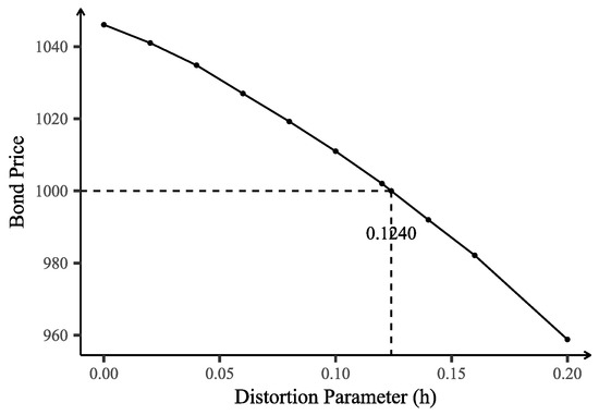
Figure 5.
Impact of distortion parameter h on bond price.
When h increases, both earthquake frequency and magnitude rise. This leads to a higher probability of triggering principal loss, which in turn lowers the bond price. In other words, when investors face higher risk or uncertainty, they demand greater yields, resulting in lower bond prices. Figure 5 shows that the bond price declines at an accelerating rate as h increases. When , the bond price exactly equals its face value, . At this point, the Poisson distribution parameter is distorted from to , and the Gamma distribution parameters change from and to and .
Table 3 summarizes the expected bond prices, their 99% confidence intervals, and sample standard deviations under a range of distortion parameter values. The results reveal a distinct trend: as the distortion parameter h increases, the expected bond price decreases, while its sample standard deviation rises. This is mainly due to the fact that a larger distortion parameter increases the probability of triggering a bond payout. Consequently, a higher proportion of simulated paths incur principal loss, thereby lowering the expected bond price. At the same time, the increased frequency of these low-price paths amplifies price volatility, as reflected by the growth in the sample standard deviation. The consistently tight confidential intervals indicate that the expected bond prices, estimated from 100,000 simulations, are highly reliable.
Table 3.
Expected bond prices with different distortion parameters based on 100,000 simulations, along with their 99% confidence intervals and sample standard deviations.
4. Discussion
4.1. Comparison of Aggregate Loss Distortion and Partial Distortion
Applying a distortion transformation to the aggregate loss distribution is mathematically equivalent to simultaneously distorting both loss frequency and loss severity distributions. Alternatively, distortion can be applied only to the frequency or only to the severity distribution. This section provides a comparative analysis of these three approaches.
As previously discussed, earthquake occurrence frequency is modeled using a Poisson distribution, i.e., . Under an Esscher transformation with distortion parameter h, the probability mass function of the distorted process becomes
This shows that the Esscher transform of the Poisson distribution with parameter yields a Poisson distribution with parameter . The effect of varying the distortion parameter h on bond prices when only the frequency distribution is distorted is illustrated in Figure 6.
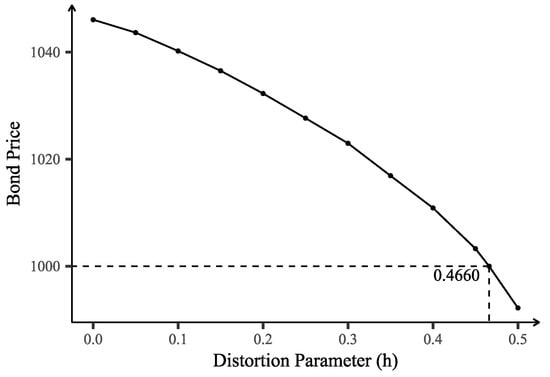
Figure 6.
Impact of distortion parameter h on bond price when distorting the frequency distribution only.
The earthquake magnitude follows a left-truncated Gamma distribution, i.e., . After applying the Esscher transform to , we obtain a Gamma distribution with parameters .
If the distortion transform is applied only to the earthquake magnitude distribution, the effect of the distortion parameter h on the bond price is shown in Figure 7.
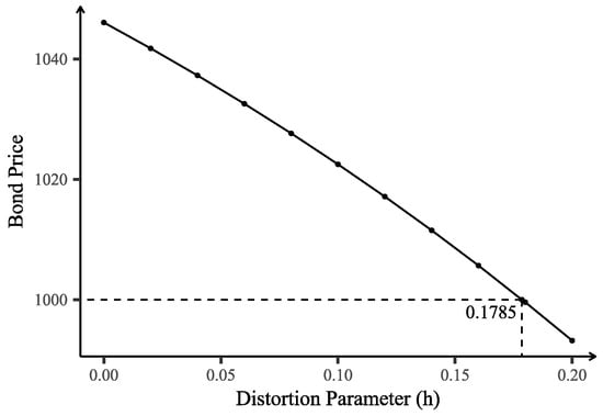
Figure 7.
Impact of distortion parameter h on bond price when distorting the severity distribution only.
The simulation results reveal that achieving a bond price equal to its face value of 1000 requires a significantly larger distortion parameter when only the frequency or only the severity distribution is distorted, compared with distorting the aggregate loss distribution. Specifically,
- Distorting only the frequency distribution requires .
- Distorting only the severity distribution requires .
- Distorting the aggregate loss distribution requires only .
These findings suggest that directly applying distortion to the aggregate loss distribution is more efficient for achieving the target pricing outcome. Moreover, this approach better preserves the underlying statistical properties of both the frequency and severity components and avoids excessive deviation from their original distributional characteristics.
4.2. Sensitive Analysis of Bond Price
When the aggregate loss distribution is distorted and the distortion parameter is set to , the resulting CAT bond price is exactly equal to its face value of 1000. Conditional on this distortion level, Figure 8 illustrates the sensitivity of the expected bond price to variations in the coupon rate, the parameters of the Gamma distribution (shape and rate ), and the Poisson distribution parameter .
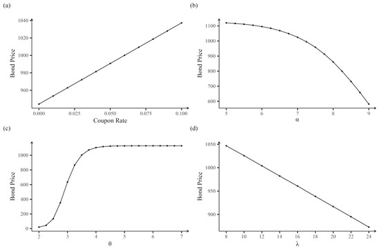
Figure 8.
Sensitivity analysis of the catastrophe bond price with respect to pricing formula parameters. Each subplot shows the change in the bond price as one parameter is varied, while all others are held constant at their baseline values. (a) Bond price as a function of the coupon rate; (b) Bond price sensitivity to the parameter ; (c) Bond price sensitivity to the parameter ; (d) Bond price sensitivity to the parameter .
As expected, the coupon rate exhibits a positive relationship with the bond price, while the Poisson parameter demonstrates a negative relationship. This is consistent with the theoretical result derived in (4), where the bond price increases linearly with respect to the fixed coupon rate. Figure 8a confirms this linear relationship, showing that as the coupon rate increases, the bond’s present value rises accordingly. The Poisson parameter represents the expected annual frequency of earthquakes exceeding magnitude 4.0. A higher value of implies a greater likelihood of triggering loss events over the bond’s term, thereby increasing the expected payout and reducing the bond’s price. Figure 8d verifies this inverse relationship, revealing an approximately linear negative sensitivity of bond price to the Poisson parameter. This is related to the design of the bond trigger mechanism.
Figure 8b,c explore the effects of changes in the Gamma distribution parameters. The sensitivity to the shape parameter is nonlinear and pronounced: as increases, the bond price declines at an accelerating rate. For the rate parameter , the bond price shows a steep but decelerating increase for , eventually plateauing when . These patterns highlight the role of the loss severity distribution in determining the probability of triggering payouts at high thresholds. The observed sensitivity to is closely tied to the specific payout design employed in this study.
4.3. Comparison of Different Distortion Operators
A generalized method proposed in [16] for constructing distortion operators, which can generalize various forms of distortion operators proposed in the existing literature, while also allowing for the use of various different distributions to construct new ones. The general form of this distortion operator is as follows:
where and are distribution functions from the same family but with different parameters, and and are their corresponding survival functions, respectively.
The Wang transform is a widely used distortion operator in finance and risk management, primarily used to reallocate risk weights by adjusting the cumulative distribution function to reflect investor risk preferences. It is defined as
where denotes the standard Normal cumulative distribution function, is its inverse function, and is the parameter that captures the degree of risk aversion. When , the Wang transform increases the weight assigned to tail risks, thereby emphasizing extreme losses; conversely, when , the tail risk is underestimated. The Wang distortion operator operates directly on the cumulative distribution function through quantile mapping, making it particularly suitable for distributions with explicit analytic forms. However, when the cumulative distribution function is complex and non-normal, the transformed distribution becomes analytically intractable, which limits its practical applicability.
The Poisson–Gamma distortion operator developed in this paper, which is derived via the Esscher transform applied to the aggregate loss distribution, can achieve a similar risk adjustment effect to the Wang transform distortion operator with certain advantages. Let the aggregate loss variable be defined as , where and . The distribution function of aggregate loss X is denoted by , and its survival function by . Specifically, the cumulative distribution function of PG distribution can be expressed as
In actual calculations, the terms can be omitted according to the accuracy requirements of .
After applying the Esscher transform with parameter h, the transformed distribution function can be expressed as
where .
According to (34), (36), and (37), the corresponding Poisson–Gamma distortion operator can be expressed as
Similarly, the distortion operator of only applying the distortion transform to the frequency distribution or severity distribution can be denoted by
The Esscher transform adjusts tail probabilities by exponentially reweighting the probability density function. For distributions that include terms of the form , the Esscher transform is not only easy to implement, but it also tends to preserve the structural form of the distribution to a large extent. This facilitates the analysis of post-transformation distribution properties and related statistics.
Figure 9 plots the distortion operator as . It can be observed that distorting only the frequency distribution results in a significantly greater shift in the aggregate loss distribution than distorting only the severity distribution. However, because bond trigger points are typically located at high quantiles, bond prices are relatively insensitive to changes in the distortion parameter when only the frequency distribution is distorted. As a result, the impact on pricing remains limited. In contrast, the distortion of the severity distribution has a much more pronounced and dominant effect on bond pricing.
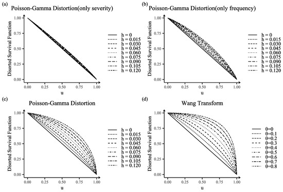
Figure 9.
Comparison of the distorted survival functions under different distortion operators. (a) Distortion applied only to the severity distribution, corresponding to (40); (b) Distortion applied only to the frequency distribution, corresponding to (39); (c) Distortion applied to the aggregate loss distribution, corresponding to (38); and (d) Distortion resulting from the Wang Transform, corresponding to (35).
Comparing Figure 9c,d, we observe both similarities and differences between the Wang transform and the proposed Poisson–Gamma distortion operator in their treatment of tail risk. The Poisson–Gamma operator can replicate the tail-weighting effects of the Wang transform through appropriate parameterization while providing greater analytical tractability for complex distributions. Comparing the Wang transform with the Esscher transform, it can be seen that both methods increase the weight of tail probabilities when the distortion parameter is positive, thus reflecting heightened concern for extreme losses. Although some connections between the two transforms have been noted (see [38,39,40]), it is difficult to obtain the transformed distribution form analytically by using the Wang transform for complex distributions, which typically requires numerical methods for implementation. By contrast, the Esscher transform, with its well-defined mathematical formulation, enables more tractable analysis of the transformed distribution and its implications for bond pricing mechanisms. This analytical advantage is particularly evident when applying the transform to aggregate loss distributions.
5. Conclusions
This study has developed a novel mathematical framework for pricing contingent claims on compound risk processes, with a direct application to the valuation of catastrophe (CAT) bonds in incomplete markets. By applying the Esscher transform to the aggregate loss distribution, the measure transformation of the compound process can be uniquely and analytically decomposed into a tractable, parametric adjustment of its underlying frequency and severity distributions. This decomposition property provides the model with significant analytical tractability, allowing for a transparent derivation of the pricing measure’s properties, offering a distinct advantage over alternative methods such as the Wang transform. As demonstrated in Section 4, the analytical structure leads to a more efficient incorporation of risk preference, requiring less parameter perturbation than partial distortion methods to achieve market-consistent pricing targets. Furthermore, the model’s applicability is validated through an empirical analysis based on Chinese earthquake data, conforming that the theoretical framework constitutes a practical and powerful tool for financial applications.
The practical implications of this model are significant. For issuers, it enhances risk quantification, leading to fairer pricing and improved capital efficiency. For investors, it increases transparency and allows for a clearer assessment of risk sensitivities, supporting more informed asset allocation. At the market level, the framework promotes a consistent and theoretically sound pricing standard, which could enhance market liquidity and ultimately strengthen societal resilience against catastrophic events.
Despite this study’s contributions, it has several limitations, which open avenues for future research. First, the model assumes that catastrophic risk and financial risk are independent of each other; future CAT pricing research could attempt to design a model under the non-independence assumption to capture the contagion effect during systemic crises. Second, the framework only considers one hazard, earthquakes, and due to limited data, it does not account for regional differences. Extending it to accommodate multi-hazard, multi-regional, or compensation-based trigger mechanisms is a key next step. Third, the Esscher transform uses only one parameter, h, to express the market’s risk aversion. Further research could also consider alternative constructs of risk-neutral measures based on behavioral finance models, such as ambiguity aversion or cumulative prospect theory (CPT), to better capture decision making under uncertainty.
Funding
This research was funded by the National Social Science Fund of China (Grant No. 22ATJ005) and the National Natural Science Foundation of China (Grant No. 72301086).
Data Availability Statement
The data presented in this study are openly available from the China Earthquake Networks Center, National Earthquake Data Center, at http://data.earthquake.cn (accessed on 1 June 2023).
Conflicts of Interest
The author declares no conflicts of interest.
References
- Newman, R.; Noy, I. The global costs of extreme weather that are attributable to climate change. Nat. Commun. 2023, 14, 6103. [Google Scholar] [CrossRef]
- Jensen, S.J.; Feldmann-Jensen, S.; Johnston, D.M.; Brown, N.A. The emergence of a globalized system for disaster risk management and challenges for appropriate governance. Int. J. Disaster Risk Sci. 2015, 6, 87–93. [Google Scholar] [CrossRef]
- Lane, M.; Mahul, O. Catastrophe Risk Pricing: An Empirical Analysis. World Bank Policy Research Working Paper No.4765. 2008. Available online: https://ssrn.com/abstract=1297804 (accessed on 12 August 2025).
- Jaffee, D.M.; Russell, T. Catastrophe insurance, capital markets, and uninsurable risks. J. Risk Insur. 1997, 64, 205–230. [Google Scholar] [CrossRef]
- Hagendorff, B.; Hagendorff, J.; Keasey, K.; Gonzalez, A. The risk implications of insurance securitization: The case of catastrophe bonds. J. Corp. Financ. 2014, 25, 387–402. [Google Scholar] [CrossRef]
- Zhao, Y.; Yu, M.T. Predicting catastrophe risk: Evidence from catastrophe bond markets. J. Bank. Financ. 2020, 121, 105982. [Google Scholar] [CrossRef]
- Cummins, J.D.; Weiss, M.A. Convergence of insurance and financial markets: Hybrid and securitized risk-transfer solutions. J. Risk Insur. 2009, 76, 493–545. [Google Scholar] [CrossRef]
- Galeotti, M.; Gürtler, M.; Winkelvos, C. Accuracy of premium calculation models for CAT bonds—An empirical analysis. J. Risk Insur. 2013, 80, 401–421. [Google Scholar] [CrossRef]
- Braun, A. Pricing in the primary market for cat bonds: New empirical evidence. J. Risk Insur. 2016, 83, 811–847. [Google Scholar] [CrossRef]
- Hamada, M.; Sherris, M. Contingent claim pricing using probability distortion operators: Methods from insurance risk pricing and their relationship to financial theory. Appl. Math. Financ. 2003, 10, 19–47. [Google Scholar] [CrossRef]
- Venter, G. Premium calculation implications of reinsurance without arbitrage. ASTIN Bull. 1991, 21, 223–230. [Google Scholar] [CrossRef]
- Wang, S. Insurance pricing and increased limits ratemaking by proportional hazards transforms. Insur. Math. Econ. 1995, 17, 43–54. [Google Scholar] [CrossRef]
- Wang, S. A class of distortion operators for pricing financial and insurance risks. J. Risk Insur. 2000, 67, 15–36. [Google Scholar] [CrossRef]
- Wang, S. A universal framework for pricing financial and insurance risks. ASTIN Bull. 2002, 32, 213–234. [Google Scholar] [CrossRef]
- Godin, F.; Mayoral, S.; Morales, M. Contingent claim pricing using a Normal Inverse Gaussian probability distortion operator. J. Risk Insur. 2012, 79, 841–866. [Google Scholar] [CrossRef]
- Godin, F.; Lai, V.S.; Trottier, D.A. A general class of distortion operators for pricing contingent claims with applications to CAT bonds. Scand. Actuar. J. 2019, 2019, 558–584. [Google Scholar] [CrossRef]
- Furman, E.; Zitikis, R. Weighted premium calculation principles. Insur. Math. Econ. 2008, 42, 459–465. [Google Scholar] [CrossRef]
- Gerber, H.U.; Shiu, E.S.W. Option pricing by Esscher transforms. Trans. Soc. Actuar. 1994, 46, 99–191. [Google Scholar]
- Cox, S.H.; Pedersen, H.W. Catastrophe risk bonds. N. Am. Actuar. J. 2000, 4, 56–82. [Google Scholar] [CrossRef]
- Huang, S.; Zhang, J.; Zhu, W. Storm CAT bond: Modeling and valuation. North Am. Actuar. J. 2024, 28, 718–743. [Google Scholar] [CrossRef]
- Eichler, A.; Leobacher, G.; Szölgyenyi, M. Utility indifference pricing of insurance catastrophe derivatives. Eur. Actuar. J. 2017, 7, 515–534. [Google Scholar] [CrossRef]
- Liu, H.; Tang, Q.; Yuan, Z. Indifference pricing of insurance-linked securities in a multi-period model. Eur. J. Oper. Res. 2021, 289, 793–805. [Google Scholar] [CrossRef]
- Anggraeni, W.; Supian, S.; Sukono; Abdul Halim, N.B. Earthquake catastrophe bond pricing using extreme value theory: A mini-review approach. Mathematics 2022, 10, 4196. [Google Scholar] [CrossRef]
- Boudreault, M.; Cossette, H.; Marceau, É. Risk models with dependence between claim occurrences and severities for Atlantic hurricanes. Insur. Math. Econ. 2014, 54, 123–132. [Google Scholar] [CrossRef]
- Albrecher, H.; Araujo-Acuna, J.C.; Beirlant, J. Fitting nonstationary Cox processes: An application to fire insurance data. N. Am. Actuar. J. 2021, 25, 135–162. [Google Scholar] [CrossRef]
- Avanzi, B.; Taylor, G.; Wong, B.; Yang, X. On the modelling of multivariate counts with Cox processes and dependent shot noise intensities. Insur. Math. Econ. 2021, 99, 9–24. [Google Scholar] [CrossRef]
- Kwon, J.; Zheng, Y.; Jun, M. Flexible spatio-temporal Hawkes process models for earthquake occurrences. Spat. Stat. 2023, 54, 100728. [Google Scholar] [CrossRef]
- Tang, Q.; Yuan, Z. CAT bond pricing under a product probability measure with POT risk characterization. ASTIN Bull. 2019, 49, 457–490. [Google Scholar] [CrossRef]
- Li, J.; Cai, Z.; Liu, Y.; Ling, C. Extremal Analysis of Flooding Risk and Its Catastrophe Bond Pricing. Mathematics 2023, 11, 114. [Google Scholar] [CrossRef]
- Sukono; Ghazali, P.L.B.; Ibrahim, R.A.; Riaman; Mamat, M.; Sambas, A.; Hidyat, Y. Price model of multiple-trigger flood bond with trigger indices of aggregate losses and maximum number of submerged houses. Int. J. Disaster Risk Reduct. 2025, 116, 105156. [Google Scholar] [CrossRef]
- Burnecki, K.; Teuerle, M.A.; Zdeb, M. Pricing of insurance-linked securities: A multi-peril approach. J. Math. Ind. 2024, 14, 14. [Google Scholar] [CrossRef]
- Domfeh, D.; Chatterjee, A.; Dixon, M. A Bayesian valuation framework for catastrophe bonds. J. R. Stat. Soc. Ser. Appl. Stat. 2024, 73, 1389–1410. [Google Scholar] [CrossRef]
- Safarveisi, S.; Domfeh, D.; Chatterjee, A. Catastrophe bond pricing under the renewal process. Scand. Actuar. J. 2025, 1–28. [Google Scholar] [CrossRef]
- Hull, J.C. Options, Futures, and Other Derivatives, 10th ed.; Pearson: Boston, MA, USA, 2018; pp. 702–712. [Google Scholar]
- Li, H.; Su, J. Mitigating wildfire losses via insurance-linked securities: Modeling and risk management perspectives. J. Risk Insur. 2024, 91, 383–414. [Google Scholar] [CrossRef]
- Ma, Z.G.; Ma, C.Q. Pricing catastrophe risk bonds: A mixed approximation method. Insur. Math. Econ. 2013, 52, 243–254. [Google Scholar] [CrossRef]
- Stupfler, G.; Yang, F. Analyzing and predicting CAT bond premiums: A financial loss premium principle and extreme value modeling. ASTIN Bull. 2018, 48, 375–411. [Google Scholar] [CrossRef]
- Kijima, M.; Muromachi, Y. An extension of the Wang transform derived from Bühlmanns economic premium principle for insurance risk. Insur. Math. Econ. 2008, 42, 887–896. [Google Scholar] [CrossRef]
- Wang, S. Normalized exponential tilting: Pricing and measuring multivariate risks. N. Am. Actuar. J. 2007, 11, 89–99. [Google Scholar] [CrossRef]
- Labuschagne, C.C.A.; Theresa, M.O. A Note on the Connection between the Esscher–Girsanov Transform and the Wang Transform. Insur. Math. Econ. 2010, 47, 385–390. [Google Scholar] [CrossRef]
Disclaimer/Publisher’s Note: The statements, opinions and data contained in all publications are solely those of the individual author(s) and contributor(s) and not of MDPI and/or the editor(s). MDPI and/or the editor(s) disclaim responsibility for any injury to people or property resulting from any ideas, methods, instructions or products referred to in the content. |
© 2025 by the author. Licensee MDPI, Basel, Switzerland. This article is an open access article distributed under the terms and conditions of the Creative Commons Attribution (CC BY) license (https://creativecommons.org/licenses/by/4.0/).