A Novel Moving Average–Exponentiated Exponentially Weighted Moving Average (MA-Exp-EWMA) Control Chart for Detecting Small Shifts

Abstract

Process monitoring plays a vital role in ensuring quality stability, and, operational efficiency across fields such as manufacturing, finance, biomedical science, and environmental monitoring. Among statistical tools, control charts are widely adopted for detecting variability and abnormal patterns. Since the introduction of the basic X-bar control chart by Shewhart in the 1920s, various improved methods have emerged to address the challenge of identifying small and latent process shifts, including CUSUM, MA, EWMA, and Exp-EWMA control charts. This study introduces a novel control chart—the Moving Average–Exponentiated Exponentially Weighted Moving Average (MA-Exp-EWMA) control chart—combining the smoothing effect of MA and the adaptive weighting of Exp-EWMA. Its goal is to improve the detection of small shifts and gradual changes. Performance is evaluated using average run length (ARL), standard deviation of run length (SDRL), and median run length (MRL). Monte Carlo simulations under different distributions (normal, exponential, gamma, and Student’s t) and parameter settings assess the control chart’s sensitivity under various shift scenarios. Comparisons with existing control charts and an application to real data demonstrate the practical effectiveness of the proposed method in detecting small shifts.

1. Introduction

Statistical Process Control (SPC) was introduced by Shewhart (1931, 1939) [1,2], who is regarded as the father of modern quality management. At the time of rapid industrialization, the manufacturing industry faced challenges of mass production and product consistency. To monitor process stability and ensure product quality, Shewhart invented the control chart, a foundational tool for SPC, during his work at Bell Telephone Laboratories. His control chart, based on statistical means and standard deviations, sets upper control limits (UCL), a center line (CL), and lower control limits (LCL), helping to intuitively identify process variation. By the mid-20th century, the Shewhart control chart became an essential tool in manufacturing, laying the foundation for subsequent quality theories such as the PDCA cycle and Total Quality Management (TQM).

In practice, SPC is widely applied beyond manufacturing—in healthcare, finance, and service industries—to monitor and improve process stability and consistency. SPC helps distinguish between assignable causes (special variation) and common causes (natural variation), enabling timely actions to reduce defective rates. Particularly in high-precision environments such as semiconductor manufacturing, aerospace, and medical device production, SPC is crucial for ensuring quality and safety. With the advancement of digital and automation technologies, SPC has been integrated into smart manufacturing, allowing early warnings of process anomalies through real-time data analysis.

Run length (RL) is one of the core concepts in SPC, used to assess a control chart’s ability to detect anomalies. Page (1961) [3] first applied RL’s statistical properties to cumulative sum control charts (CUSUM), introducing average run length (ARL) to quantify detection performance. ARL includes $AR{L}_0$ and $AR{L}_1$, describing false alarm rates under stable processes and sensitivity under out-of-control processes, respectively. Roberts (1970) [4] noted that ARL alone was insufficient for comprehensive performance evaluation and proposed the standard deviation of run length (SDRL) to describe the variability of RL. A lower SDRL indicates more stable detection results and reflects better consistency in monitoring. Furthermore, Xie et al. (2000) [5] introduced the median run length (MRL), which uses the RL median to mitigate the influence of extreme values, making it particularly suitable in asymmetric or long-tailed distributions. In addition to these classical measures, recent research (e.g., Paichit and Peerajit, 2022 [6]; Talordphop et al., 2025 [7]; Makaew et al., 2025 [8]) continues to expand RL-based performance evaluations for newly proposed control charts. These studies confirm that RL-based metrics remain central in verifying the performance of advanced control chart designs.

As industries progressed, the Shewhart control chart’s limited sensitivity to small process shifts led to various enhancements. Roberts (1959) [9] proposed the Exponentially Weighted Moving Average (EWMA) control chart, which improves the detection of small variations by assigning exponentially decreasing weights to past data. Khoo (2004) [10] introduced the Moving Average (MA) control chart, which smooths out random process noise and highlights long-term trends. These methods advanced control chart accuracy and marked a shift toward combining dynamic weighting techniques.

Based on EWMA, Taboran et al. (2019) [11] proposed the MA-EWMA control chart, combining the smoothing property of MA with the sensitivity of EWMA to enhance the detection of short- and long-term shifts. In response to increasing data complexity, Alevizakos et al. (2024) [12] introduced the Exponentiated Exponentially Weighted Moving Average (Exp-EWMA) control chart. This method incorporates a dynamic smoothing parameter, adjusting the weighting factor through an exponential function to adapt to different stages of the process. The evolution of SPC not only demonstrates the practical potential of statistics but also reflects continuous advancements in quality management from the industrial age to modern automation.

With the ongoing development of control chart techniques, improving the ability to detect small or gradual shifts while maintaining stability remains a critical issue in SPC. Among existing methods, the MA-EWMA control chart has shown good performance in many monitoring applications by combining MA’s smoothing effect with EWMA’s sensitivity, effectively addressing both short-term noise suppression and long-term trend detection. On the other hand, the Exp-EWMA control chart introduces dynamic parameter adjustment via an exponential function, allowing adaptive responses to different stages of the process and improving early anomaly detection.

While MA-EWMA control charts offer strengths in stability and smoothing, Exp-EWMA control charts provide dynamic weighting and enhanced sensitivity. Despite these advantages, both methodologies face limitations under certain conditions, such as delayed detection of incipient shifts or inconsistent false alarm control. This study proposes a novel control chart, MA-Exp-EWMA. The motivation for combining MA with Exp-EWMA lies in leveraging their complementary strengths: the MA component smooths out short-term noise and highlights long-term trends, while the Exp-EWMA component adaptively adjusts weights to improve sensitivity to small and gradual shifts. By integrating these two features, the proposed MA-Exp-EWMA chart enhances detection performance without sacrificing stability.

Through methodological innovation, this research seeks to overcome the limitations of static weighting and fixed smoothing in current control charts, offering a monitoring tool that can respond to different types of variation and data structures, thus improving the timeliness and accuracy of overall process quality control.

The remainder of this article is organized as follows. Section 2 elaborates on existing control charts, including the characteristics and limitations of traditional and improved control charts. Section 3 describes the framework and mathematical formulation of the proposed MA-Exp-EWMA control chart. Section 4 uses Monte Carlo simulations to evaluate detection ability under different distributions and parameter settings, and compares performance against other control charts to assess stability and sensitivity. Section 5 applies two real-world datasets with time-series characteristics to test anomaly detection and compare results, validating the practical applicability of the control chart. Section 6 provides conclusions and future directions, summarizing findings and discussing the balance between stability and sensitivity of the control chart, along with its potential and future improvements across different data types and applications.

2. Existing Control Charts

2.1. EWMA Control Chart

With industrial development, the need for early detection of small process shifts has grown. Roberts (1959) [9] proposed the concept of the EWMA and applied it to control chart construction.

The EWMA control chart enhances sensitivity to small shifts by computing the Exponentially Weighted Moving Average $Z_t$, where $Z_t$ at time t is defined as follows:

$$Z_t=\lambda X_t+(1-\lambda )Z_{t-1},t=1,2,3,\dots$$

assuming $X_t$ is an independent random variable with mean $\mu$ and variance ${\sigma }^2$, $\lambda$ is the smoothing parameter ($0<\lambda \le 1$), controlling the influence of recent versus historical data. The initial value $Z_0$ is set to the process target $\mu$. The statistic $Z_t$ combines both historical and current data, assigning different weights to past and new observations.

By expanding the recursion, we obtain the following:

$$\begin{array}{cc}\hfill Z_t& =\lambda \sum _{j=0}^{t-1}{(1-\lambda )}^j{X}_{t-j}+{(1-\lambda )}^t\mu \hfill \end{array}$$

(1)

The above expansion shows that the weights for past data $\lambda {(1-\lambda )}^j$ decay geometrically over time. The total sum of weights is as follows:

$$\begin{array}{ccc}\hfill \lambda \sum _{j=0}^{t-1}{(1-\lambda )}^j+{(1-\lambda )}^t& =\lambda ·{\displaystyle \frac{1-{(1-\lambda )}^t}{\lambda }}+{(1-\lambda )}^t\hfill & \hfill =1\end{array}$$

Thus, the total weight sums to 1, ensuring that the statistic $Z_t$ remains a balanced weighted average rather than a biased linear combination. Assuming $X_t$ is an independent random variable with variance ${\sigma }^2$, the expectation of $Z_t$ is $E\left(Z_t\right)=\mu$ and the variance of $Z_t$ is $\mathrm{Var}\left(Z_t\right)={\displaystyle \frac{\lambda }{2-\lambda }}\left[1-{(1-\lambda )}^{2t}\right]{\sigma }^2$. As $t\to \infty$, ${(1-\lambda )}^{2t}\to 0$, thus $\mathrm{Var}\left(Z_t\right)={\displaystyle \frac{\lambda }{2-\lambda }}{\sigma }^2$.

The control limits and the centerline of the EWMA control chart are defined as follows:

$$\left\{\begin{array}{cc}\hfill \mathrm{UCL}& =\mu +L\sigma \sqrt{{\displaystyle \frac{\lambda }{2-\lambda }}\left[1-{(1-\lambda )}^{2t}\right]},\hfill \\ \hfill \mathrm{CL}& =\mu ,\hfill \\ \hfill \mathrm{LCL}& =\mu -L\sigma \sqrt{{\displaystyle \frac{\lambda }{2-\lambda }}\left[1-{(1-\lambda )}^{2t}\right]},\hfill \end{array}\right.$$

(2)

where L is the control limit coefficient.

As time t increases, $[1-{(1-\lambda )}^{2t}]$ approaches 1. Equation (2) then reaches a steady state:

$$\left\{\begin{array}{cc}\hfill \mathrm{UCL}& =\mu +L\sigma \sqrt{{\displaystyle \frac{\lambda }{2-\lambda }}},\hfill \\ \hfill \mathrm{CL}& =\mu ,\hfill \\ \hfill \mathrm{LCL}& =\mu -L\sigma \sqrt{{\displaystyle \frac{\lambda }{2-\lambda }}}.\hfill \end{array}\right.$$

2.2. MA Control Chart

In the field of statistical quality control, the concept of MA can be traced back to Duncan (1986) [13]. He applied Moving Average techniques to process monitoring, emphasizing their role in smoothing random fluctuations and highlighting process trends, thus serving as a fundamental tool for analyzing process stability.

Building upon this, Khoo (2004) [10] extended the MA method, proposing a MA control chart specifically designed to monitor the fraction non-conforming. Assuming that the observations $X_t$ are independent and identically distributed random variables with mean $\mu$ and variance ${\sigma }^2$, let $M_t$ be the MA statistic at time t with a window size of w, defined as follows:

$$M_t=\left\{\begin{array}{cc}{\displaystyle \frac{X_t+X_{t-1}+\dots +X_{t-w+1}}{w}},\hfill & \mathrm{if}t\ge w,\hfill \\ {\displaystyle \frac{X_t+X_{t-1}+\dots +X_1}{t}},\hfill & \mathrm{if}t<w.\hfill \end{array}\right.$$

(3)

when $t\ge w$, the expectation and variance of $M_t$ are $E\left(M_t\right)=\mu$ and $\mathrm{Var}\left(M_t\right)={\displaystyle \frac{{\sigma }^2}{w}}$. When $t<w$, the expectation and variance of $M_t$ are $E\left(M_t\right)=\mu$ and $\mathrm{Var}\left(M_t\right)={\displaystyle \frac{{\sigma }^2}{t}}$. Therefore, the control limits and the centerline of the MA control chart are defined as follows:

$$\left\{\begin{array}{cc}\hfill \mathrm{UCL}& =\mu +L{\displaystyle \frac{\sigma }{\sqrt{w}}},\hfill \\ \hfill \mathrm{CL}& =\mu \hfill & \hfill ,t\ge w\\ \hfill \mathrm{LCL}& =\mu -L{\displaystyle \frac{\sigma }{\sqrt{w}}},\hfill \end{array}\right.$$

or

$$\left\{\begin{array}{cc}\hfill \mathrm{UCL}& =\mu +L{\displaystyle \frac{\sigma }{\sqrt{t}}},\hfill \\ \hfill \mathrm{CL}& =\mu \hfill & \hfill ,1\le t<w\\ \hfill \mathrm{LCL}& =\mu -L{\displaystyle \frac{\sigma }{\sqrt{t}}},\hfill \end{array}\right.$$

where L is the control limit coefficient.

2.3. Exp-EWMA Control Chart

The Exp-EWMA control chart is an improved version of the EWMA control chart, proposed by Alevizakos et al. (2024) [12]. This method builds on traditional EWMA theory by designing an exponential function as the smoothing parameter, allowing it to vary over time.

The core of the Exp-EWMA control chart is the time-varying smoothing parameter $\lambda \left(t\right)$. Assume that $X_t$ is an independent random variable with expectation $\mu$ and variance ${\sigma }^2$. The recursive formula of the statistic is defined as follows:

$$Z_t=\lambda \left(t\right)X_t+\left(1-\lambda \left(t\right)\right)Z_{t-1},$$

(4)

where

$$\lambda \left(t\right)=e^{-f\left(t\right)},f\left(t\right)=-ln\left(\lambda \right)+a^{\left(c+{\displaystyle \frac{1}{t}}\right)},$$

and $\lambda$ is the base smoothing parameter ($0<\lambda \le 1$), while a and c are design parameters that control the rate of change in the smoothing parameter. Expanding Equation (4) recursively with $Z_0=\mu$ results in the following:

$$\begin{array}{cc}\hfill Z_t& =\lambda e^{-a^{\left(c+{\displaystyle \frac{1}{t}}\right)}}{X}_t+\sum _{i=1}^{t-1}\lambda e^{-a^{\left(c+{\displaystyle \frac{1}{i}}\right)}}\prod _{j=i}^{t-1}\left(1-\lambda e^{-a^{\left(c+{\displaystyle \frac{1}{j+1}}\right)}}\right)X_i+\prod _{j=1}^t\left(1-\lambda e^{-a^{\left(c+{\displaystyle \frac{1}{j}}\right)}}\right)\mu .\hfill \end{array}$$

(5)

Assuming that $X_t$ is an independent random variable with variance ${\sigma }^2$, the expectation of the statistic $Z_t$ from Equation (5) is as follows:

$$\begin{array}{cc}\hfill E\left(Z_t\right)& =\lambda e^{-a^{\left(c+{\displaystyle \frac{1}{t}}\right)}}E\left(X_t\right)+\sum _{i=1}^{t-1}\lambda e^{-a^{\left(c+{\displaystyle \frac{1}{i}}\right)}}\left(\prod _{j=i}^{t-1}\left(1-\lambda e^{-a^{\left(c+{\displaystyle \frac{1}{j+1}}\right)}}\right)\right)E\left(X_i\right)\hfill \\ & +\prod _{j=1}^t\left(1-\lambda e^{-a^{\left(c+{\displaystyle \frac{1}{j}}\right)}}\right)\mu \hfill \\ & =\left[\lambda e^{-a^{\left(c+{\displaystyle \frac{1}{t}}\right)}}+\sum _{i=1}^{t-1}\lambda e^{-a^{\left(c+{\displaystyle \frac{1}{i}}\right)}}\left(\prod _{j=i}^{t-1}\left(1-\lambda e^{-a^{\left(c+{\displaystyle \frac{1}{j+1}}\right)}}\right)\right)\right.\hfill \\ & \left.+\prod _{j=1}^t\left(1-\lambda e^{-a^{\left(c+{\displaystyle \frac{1}{j}}\right)}}\right)\right]\mu \hfill \\ & =\left[\lambda e^{-a^{\left(c+{\displaystyle \frac{1}{t}}\right)}}+\sum _{i=1}^{t-1}\left[\left(\prod _{j=i+1}^t\left(1-\lambda e^{-a^{\left(c+{\displaystyle \frac{1}{j}}\right)}}\right)\right)-\left(\prod _{j=i}^t\left(1-\lambda e^{-a^{\left(c+{\displaystyle \frac{1}{j}}\right)}}\right)\right)\right]\right.\hfill \\ & \left.+\prod _{j=1}^t\left(1-\lambda e^{-a^{\left(c+{\displaystyle \frac{1}{j}}\right)}}\right)\right]\mu =\mu \hfill \end{array}$$

the variance of $Z_t$ is given by the following:

$$\begin{array}{cc}\hfill \mathrm{Var}\left(Z_t\right)& =\left[{\left(\lambda e^{-a^{\left(c+{\displaystyle \frac{1}{t}}\right)}}\right)}^2+\sum _{i=1}^{t-1}{\left\{\lambda e^{-a^{\left(c+{\displaystyle \frac{1}{i}}\right)}}\left(\prod _{j=i}^{t-1}\left(1-\lambda e^{-a^{\left(c+{\displaystyle \frac{1}{j+1}}\right)}}\right)\right)\right\}}^2\right]{\sigma }^2.\hfill \end{array}$$

the control limits and the centerline of the Exp-EWMA control chart are defined as follows:

$$\left\{\begin{array}{cc}\hfill \mathrm{UCL}& =\mu +L\sqrt{\mathrm{Var}\left(Z_t\right)},\hfill \\ \hfill \mathrm{CL}& =\mu ,\hfill \\ \hfill \mathrm{LCL}& =\mu -L\sqrt{\mathrm{Var}\left(Z_t\right)},\hfill \end{array}\right.$$

where L is the control limit coefficient.

2.4. MA-EWMA Control Chart

The MA-EWMA control chart was proposed by Taboran et al. (2019) [11]. It is a statistical tool that combines the features of MA and EWMA, used for monitoring parameter changes in a process.

Assume the observed value $X_t$ is an independent random variable with expectation $\mu$ and variance ${\sigma }^2$, and $X_0$ is the process target value $\mu$. Let $Z_t$ be the EWMA statistic at time t, as defined by Equation (1):

$$Z_t=\lambda \sum _{j=0}^{t-1}{(1-\lambda )}^j{X}_{t-j}+{(1-\lambda )}^t\mu ,0\le \lambda \le 1,$$

based on $Z_t$, the Moving Average is computed by substituting $Z_t$ into the MA model. The MA-EWMA statistic $M_t$ with window size w at time i is defined as follows:

$$M_t={\displaystyle \frac{Z_t+Z_{t-1}+\dots +Z_{t-w+1}}{w}},w>0.$$

the expected value of $M_t$ is as follows:

$$\begin{array}{cc}\hfill E\left(M_t\right)& =E\left[{\displaystyle \frac{Z_t+Z_{t-1}+\dots +Z_{t-w+1}}{w}}\right],\hfill \\ & ={\displaystyle \frac{1}{w}}\sum _{j=t-w+1}^{t}E\left(Z_j\right),\hfill \\ & ={\displaystyle \frac{1}{w}}\sum _{j=t-w+1}^t\left[\lambda \sum _{p=0}^{j-1}{(1-\lambda )}^{p}E\left(X_{j-p}\right)+{(1-\lambda )}^j\mu \right].\hfill \end{array}$$

the variance of $M_t$ is as follows:

$$\begin{array}{cc}\hfill \mathrm{Var}\left(M_t\right)& ={\displaystyle \frac{1}{w^2}}\sum _{j=t-w+1}^t\mathrm{Var}\left(Z_j\right),\hfill \\ & ={\displaystyle \frac{1}{w^2}}\sum _{j=t-w+1}^t\left[{\lambda }^2\sum _{p=0}^{j-1}{(1-\lambda )}^{2p}{\sigma }^2\right].\hfill \end{array}$$

therefore, the control limits and the centerline of the MA-EWMA control chart are defined as follows:

$$\left\{\begin{array}{cc}\hfill \mathrm{UCL}& =\mu +L\sqrt{{\displaystyle \frac{1}{w^2}}\sum _{j=i-w+1}^i{\lambda }^2\sum _{p=0}^{j-1}{(1-\lambda )}^{2p}{\sigma }^2},\hfill \\ \hfill \mathrm{CL}& =\mu ,\hfill \\ \hfill \mathrm{LCL}& =\mu -L\sqrt{{\displaystyle \frac{1}{w^2}}\sum _{j=i-w+1}^i{\lambda }^2\sum _{p=0}^{j-1}{(1-\lambda )}^{2p}{\sigma }^2}.\hfill \end{array}\right.$$

where L is the control limit coefficient.

3. Methods

This study builds on the Exp-EWMA control chart by Alevizakos et al. (2024) [12] and the MA-EWMA method by Taboran et al. (2019) [11], combining Exp-EWMA and MA to construct the MA-Exp-EWMA control chart. This design aims to enhance process monitoring by balancing sensitivity and stability. The integration also draws on the MA-GWMA framework by Tang (2024) [14], improving detection of small shifts.

MA-Exp-EWMA Control Chart

The MA-Exp-EWMA control chart integrates the MA and Exp-EWMA control charts. Its concept is to apply an Exponentiated Exponentially Weighted Moving Average through the Exp-EWMA model, followed by calculating the Moving Average using the MA model.

Assume that $X_t$ is an independent random variable with mean $\mu$ and variance ${\sigma }^2$. The core of the Exp-EWMA control chart lies in the smoothing function $\lambda \left(t\right)$, which varies with time t. The recursive formula for the statistic is as follows:

$$\begin{array}{cc}\hfill Z_t& =\lambda \left(t\right)X_t+\left(1-\lambda \left(t\right)\right)Z_{t-1}\hfill \\ & =\lambda e^{-a^{\left(c+{\displaystyle \frac{1}{t}}\right)}}{X}_t+\sum _{i=1}^{t-1}\lambda e^{-a^{\left(c+{\displaystyle \frac{1}{i}}\right)}}\prod _{j=i}^{t-1}\left(1-\lambda e^{-a^{\left(c+{\displaystyle \frac{1}{j+1}}\right)}}\right)X_i\hfill \\ & +\prod _{j=1}^t\left(1-\lambda e^{-a^{\left(c+{\displaystyle \frac{1}{j}}\right)}}\right)\mu .\hfill \end{array}$$

where

$$\lambda \left(t\right)=e^{-f\left(t\right)},f\left(t\right)=-ln\left(\lambda \right)+a^{\left(c+{\displaystyle \frac{1}{t}}\right)}$$

here, $\lambda$ is the smoothing parameter ($0<\lambda \le 1$), and a and c are design parameters used to adjust the rate of change in the smoothing parameter.

Based on $Z_t$ being substituted into Equation (3) for Moving Average calculation, the statistic $M_t$ at time t under the MA-Exp-EWMA control chart with window size w is defined as follows:

$$M_t=\left\{\begin{array}{cc}{\displaystyle \frac{Z_t+Z_{t-1}+\dots +Z_{t-w+1}}{w}},\hfill & \mathrm{if}t\ge w,\hfill \\ {\displaystyle \frac{Z_t+Z_{t-1}+\dots +Z_1}{t}},\hfill & \mathrm{if}t<w.\hfill \end{array}\right.$$

The expectation of the statistic $M_t$ is as follows:

$$\begin{array}{cc}\hfill E\left(M_t\right)& =E\left({\displaystyle \frac{Z_t+Z_{t-1}+\dots +Z_{t-w+1}}{w}}\right)={\displaystyle \frac{1}{w}}\sum _{j=t-w+1}^{t}E\left(Z_j\right)\hfill \\ & ={\displaystyle \frac{1}{w}}\sum _{j=t-w+1}^{t}E[\lambda e^{-a^{\left(c+{\displaystyle \frac{1}{j}}\right)}}{X}_j+\sum _{i=1}^{j-1}\lambda e^{-a^{\left(c+{\displaystyle \frac{1}{i}}\right)}}\left(\prod _{p=i}^{j-1}\left(1-\lambda e^{-a^{\left(c+{\displaystyle \frac{1}{p+1}}\right)}}\right)\right)X_i\hfill \\ & +\prod _{p=1}^j\left(1-\lambda e^{-a^{\left(c+{\displaystyle \frac{1}{p}}\right)}}\right)\mu ].\hfill \\ & ={\displaystyle \frac{1}{w}}\sum _{j=t-w+1}^t(\lambda e^{-a^{\left(c+{\displaystyle \frac{1}{j}}\right)}}E\left[X_j\right]+\sum _{i=1}^{j-1}\lambda e^{-a^{\left(c+{\displaystyle \frac{1}{i}}\right)}}\left(\prod _{p=i}^{j-1}\left(1-\lambda e^{-a^{\left(c+{\displaystyle \frac{1}{p+1}}\right)}}\right)\right)E\left[X_i\right]\hfill \\ & +\prod _{p=1}^j\left(1-\lambda e^{-a^{\left(c+{\displaystyle \frac{1}{p}}\right)}}\right)\mu ).\hfill \\ & ={\displaystyle \frac{\mu }{w}}\sum _{j=t-w+1}^t(\lambda e^{-a^{\left(c+{\displaystyle \frac{1}{j}}\right)}}+\sum _{i=1}^{j-1}\lambda e^{-a^{\left(c+{\displaystyle \frac{1}{i}}\right)}}\left(\prod _{p=i}^{j-1}\left(1-\lambda e^{-a^{\left(c+{\displaystyle \frac{1}{p+1}}\right)}}\right)\right)\hfill \\ & +\prod _{p=1}^j\left(1-\lambda e^{-a^{\left(c+{\displaystyle \frac{1}{p}}\right)}}\right)).\hfill \\ & ={\displaystyle \frac{\mu }{w}}\sum _{j=t-w+1}^t(\lambda e^{-a^{\left(c+{\displaystyle \frac{1}{tj}}\right)}}+\sum _{i=1}^{j-1}\left[\prod _{p=i+1}^j\left(1-\lambda e^{-a^{\left(c+{\displaystyle \frac{1}{p}}\right)}}\right)-\prod _{p=i}^t\left(1-\lambda e^{-a^{\left(c+{\displaystyle \frac{1}{p}}\right)}}\right)\right]\hfill \\ & +\prod _{p=1}^j\left(1-\lambda e^{-a^{\left(c+{\displaystyle \frac{1}{p}}\right)}}\right)).\hfill \\ & ={\displaystyle \frac{\mu }{w}}\sum _{j=t-w+1}^t(\lambda e^{-a^{\left(c+{\displaystyle \frac{1}{j}}\right)}}-\prod _{p=1}^j\left(1-\lambda e^{-a^{\left(c+{\displaystyle \frac{1}{p}}\right)}}\right)+\left(1-\lambda e^{-a^{\left(c+{\displaystyle \frac{1}{p}}\right)}}\right)\hfill \\ & +\prod _{p=1}^j\left(1-\lambda e^{-a^{\left(c+{\displaystyle \frac{1}{p}}\right)}}\right))={\displaystyle \frac{\mu }{w}}w=\mu \hfill \end{array}$$

The variance of the statistic $M_t$ is as follows:

$$\begin{array}{cc}\hfill \mathrm{Var}\left(M_t\right)& =\mathrm{Var}\left({\displaystyle \frac{Z_t+Z_{t-1}+\dots +Z_{t-w+1}}{w}}\right)\hfill \\ & ={\displaystyle \frac{1}{w^2}}\sum _{j=t-w+1}^t\mathrm{Var}\left(Z_j\right)\hfill \\ & ={\displaystyle \frac{1}{w^2}}\sum _{j=t-w+1}^t\mathrm{Var}[\lambda e^{-a^{\left(c+{\displaystyle \frac{1}{j}}\right)}}{X}_j+\sum _{i=1}^{j-1}\lambda e^{-a^{\left(c+{\displaystyle \frac{1}{i}}\right)}}\left(\prod _{p=i}^{j-1}\left(1-\lambda e^{-a^{\left(c+{\displaystyle \frac{1}{p+1}}\right)}}\right)\right)X_i\hfill \\ & +\prod _{p=1}^j\left(1-\lambda e^{-a^{\left(c+{\displaystyle \frac{1}{p}}\right)}}\right)\mu ].\hfill \\ & ={\displaystyle \frac{1}{w^2}}\sum _{j=t-w+1}^t\left[{\left(\lambda e^{-a^{\left(c+{\displaystyle \frac{1}{j}}\right)}}\right)}^2+\sum _{i=1}^{j-1}{\left\{\lambda e^{-a^{\left(c+{\displaystyle \frac{1}{i}}\right)}}\left(\prod _{j=i}^{j-1}\left(1-\lambda e^{-a^{\left(c+{\displaystyle \frac{1}{j+1}}\right)}}\right)\right)\right\}}^2\right]{\sigma }^2.\hfill \end{array}$$

The control limits and the centerline of the MA-Exp-EWMA control chart are defined as follows:

$$\left\{\begin{array}{cc}\hfill \mathrm{UCL}& =\mu +L\sqrt{\mathrm{Var}\left(M_t\right)},\hfill \\ \hfill \mathrm{CL}& =\mu ,\hfill \\ \hfill \mathrm{LCL}& =\mu -L\sqrt{\mathrm{Var}\left(M_t\right)},\hfill \end{array}\right.$$

where L is the control limit coefficient.

Following Alevizakos et al. (2024) [12], the baseline parameter settings $(\lambda ,a,c)$ are adopted to ensure comparability with the existing Exp-EWMA literature. The parameter $\lambda$ controls the underlying level of smoothing, while a and c govern the rate of exponential change over time. Smaller values of $(a,c)$ yield slower adaptation, emphasizing stability, whereas larger values increase responsiveness to shifts. This formulation provides flexibility in balancing sensitivity and robustness, which becomes especially important when the dynamic $\lambda \left(t\right)$ is embedded in the proposed MA-Exp-EWMA chart. In this study, we follow the settings recommended in Alevizakos et al. (2024) [12], while also noting in Section 4 that different values yield consistent trends in chart performance.

By embedding the dynamic $\lambda \left(t\right)$ into the Moving Average framework, the MA-Exp-EWMA chart inherits both the stability of MA smoothing and the adaptability of time-varying exponential weighting. This combination reduces short-term noise while retaining responsiveness to process changes, which leads to earlier detection of both gradual and sudden shifts. We note that the design parameters are not re-optimized for the MA-Exp-EWMA chart; instead, the values from Exp-EWMA are adopted to ensure a fair basis for comparison, allowing the observed performance improvements to be attributed directly to the integration of the Moving Average mechanism.

4. Simulation Study

This section conducts simulation experiments to evaluate and compare the detection performance of various parameter settings and control chart methods, thereby verifying the practicality and superiority of the proposed method. Section 4.1 describes how to use simulation to determine the appropriate control limit L under different parameter combinations such that the $AR{L}_0$ approximates the target value of 370. Section 4.2 introduces the adopted Monte Carlo simulation method, including sample generation, algorithmic procedure, and the computation of evaluation metrics. In Section 4.3, extensive simulations are conducted under four common distributions (normal, exponential, gamma, and t-distribution), considering various parameter combinations and examining performance metrics such as $AR{L}_1$, SDRL, and MRL under different shifts to select suitable parameter settings for practical use. Finally, Section 4.4 compares multiple control charts, including the proposed MA-Exp-EWMA control chart, to assess their detection capability and stability under various distributions.

4.1. Selection of Control Limits

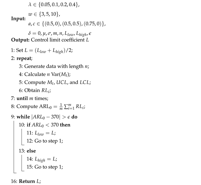
To establish a fair comparison baseline under different parameter settings, this study designs suitable control limits L for each control chart to achieve an in-control average run length of $AR{L}_0\approx 370$. This is accomplished through Monte Carlo simulation, utilizing a data length of $n=7500$, number of simulations m = 50,000 and tolerance $ϵ=1$ to ensure stability and accuracy in the estimation. The choice of m = 50,000 ensures stable estimates of run length measures while keeping the computational burden manageable.

The control limit L is determined through iterative trials and adjustments. The procedure is as follows. First, specify a lower and upper bound $L_{low}$ and $L_{high}$, and take their average as the initial value $L=(L_{low}+L_{high})/2$. Substitute L into the simulation to calculate the corresponding $AR{L}_0$. If the result shows $AR{L}_0<370$, indicating that L is too small and the control chart is too sensitive, then update the lower bound to $L_{low}=L$. Conversely, if $AR{L}_0>370$, update the upper bound to $L_{high}=L$. Repeat this bisection procedure until the simulated $AR{L}_0$ falls within the $ϵ$ tolerance of the target. The simulation procedure is detailed in Algorithm 1.

Algorithm 1: Simulation Procedure for Determining the Control Limit L.

4.2. Simulation Procedure

This subsection adopts the Monte Carlo simulation method to assess the detection performance of various control charts under different shifts $\delta$, parameter settings, and distributions. The simulation uses the control limit L obtained in Section 4.1, with m = 50,000 simulations and data length $n=7500$, ensuring statistical stability and accuracy.

For each shift $\delta$, simulations yield the run length (RL)—the number of observations from the shift to the first alarm. The average run length ${\mathrm{ARL}}_1$ reflects detection speed, and its standard deviation SDRL assesses stability. Given the skewness of RL distributions, the median run length MRL is also reported. These metrics jointly assess performance, as summarized in Algorithm 2.

Algorithm 2: Simulation Procedure for ${\mathrm{ARL}}_1$, SDRL, and MRL.
Input:	$w,\lambda ,a,c,m,n,\mu ,\sigma ,$
	$\delta \in \{0.05,0.10,0.25,0.50,1.00,2.00,3.00\}$
Output: ${\mathrm{ARL}}_1$, SDRL, and MRL under different shifts $\delta$
1: Set L by Algorithm 1;
2: repeat;
3: Generate data with different shifts $\delta$;
4: Calculate n Var($M_t$);
5: Compute $M_t$, $UCL$, and $LCL$ for each control chart;
6: Obtain $R{L}_i$;
7: until m times;
8: Compute ${\mathrm{ARL}}_1={\displaystyle \frac{1}{m}}{\sum }_{i=1}^{m}R{L}_i$;
9: Compute $\mathrm{SDRL}=\sqrt{{\displaystyle \frac{1}{m-1}}{\sum }_{i=1}^m{(R{L}_i-\mathrm{ARL})}^2}$;
10: Compute $\mathrm{MRL}=\mathrm{Median}\left(R{L}_i\right)$;
11: return ${\mathrm{ARL}}_1$, SDRL, and MRL;

4.3. Simulation Results

This section conducts simulation experiments under various distributional scenarios to evaluate the impact of different parameter settings on the detection performance of control charts, providing a basis for parameter selection in practical applications. Four different data distributions are considered: standard normal distribution $N(0,1)$, exponential distribution $Exp\left(1\right)$, gamma distribution $Gamma(4,1)$, and Student’s t-distribution $t_{10}$.

The selection of these four distributions was intended to evaluate the robustness of control charts across diverse data structures. The standard normal distribution $N(0,1)$ serves as the baseline for symmetric. To assess performance under heavy tails, we include the Student’s t-distribution with 10 degrees of freedom, following the approach of Zou and Tsung (2011) [15]. For skewed data, which are often present in practical processes, we adopt the $Exp\left(1\right)$ and the $Gamma(4,1)$ distributions, representing high and moderate right skewness, respectively, both of which were used in the study by Talordphop et al. (2022) [16].

In the simulation setup, three combinations of $(a,c)$ are considered: (0.5, 0), (0.5, 0.5), and (0.75, 0). The window size w is set to 3, 5, and 10; and the smoothing parameter $\lambda$ is set to 0.05, 0.1, 0.2, and 0.4. Simulations are performed using these combinations to evaluate how different parameters affect detection performance.

First, Algorithm 1 from Section 4.1 is used to determine the appropriate control limit L, aiming for an average run length of approximately $AR{L}_0\approx 370$ under in-control conditions. Then, under various shift magnitudes $\delta =\{0.05,0.1,0.25,0.5,1,2,3\}$, Algorithm 2 is used to evaluate $AR{L}_1$, SDRL, and MRL under each configuration. These indicators help analyze the stability and sensitivity of each parameter combination in detecting anomalies, guiding parameter selection in real data applications.

4.3.1. Normal Distribution

Based on

Table 1. Results under $N(0,1)$ with $w=3$, varying $(a,c)$ and $\lambda$.

		$\mathit{\lambda }=0.05$			$\mathit{\lambda }=0.1$			$\mathit{\lambda }=0.2$			$\mathit{\lambda }=0.4$
$(\mathit{a},\mathit{c})$	Shift($\mathbf{\delta }$)	ARL	SDRL	MRL	ARL	SDRL	MRL	ARL	SDRL	MRL	ARL	SDRL	MRL
$(0.5,0)$	0	370.31	387.34	249	369.81	372.05	254	369.15	364.89	256	369.12	360.64	257
	0.05	288.64	295.52	197	302.09	300.16	212	327.24	317.46	230	325.19	317.61	227
	0.10	178.54	172.89	125	204.97	194.57	144	228.82	222.21	163	250.97	246.48	171
	0.25	56.50	44.19	45	64.37	51.43	50	76.17	66.24	56	90.24	81.03	65
	0.50	21.70	12.99	18	23.42	14.04	20	25.84	16.48	21	28.45	20.81	22
	1.00	9.77	3.49	9	10.29	3.68	10	10.51	3.67	10	10.45	3.94	10
	2.00	5.33	1.12	5	5.57	1.17	5	5.64	1.20	5	5.41	1.20	5
	3.00	3.89	0.64	4	4.06	0.66	4	4.08	0.66	4	3.86	0.67	4
$(0.5,0.5)$	0	368.25	403.08	253	369.43	379.24	250	369.85	371.99	257	369.43	364.07	259
	0.05	299.22	311.96	200	311.73	312.79	215	332.49	329.48	232.5	343.83	348.35	237
	0.10	187.01	189.40	130	211.71	206.97	150	242.45	240.78	168	275.82	267.35	196
	0.25	58.12	50.76	45	67.43	58.40	51	85.75	79.06	62	112.28	107.99	79.5
	0.50	20.13	14.40	17	22.30	15.76	18	25.82	19.82	20	33.69	28.62	25
	1.00	7.21	3.85	6	7.80	4.19	7	8.39	4.56	7	9.09	5.42	8
	2.00	3.50	0.87	3	3.66	0.89	4	3.75	0.96	4	3.71	1.02	4
	3.00	2.59	0.58	3	2.71	0.59	3	2.76	0.60	3	2.63	0.61	3
$(0.75,0)$	0	369.24	401.66	240	369.81	389.99	256	370.47	370.76	259	369.35	364.28	263
	0.05	289.07	307.15	191	304.37	311.59	206	323.02	325.11	223	335.14	333.84	231
	0.10	174.23	174.20	121	203.43	203.23	140	230.37	229.93	161	259.84	252.86	184
	0.25	53.62	46.74	41	62.76	53.87	49	76.13	68.33	56	100.89	94.17	73
	0.50	18.73	13.77	15	21.27	15.09	18	24.00	17.75	20	29.52	23.71	23
	1.00	6.91	3.73	6	7.65	4.03	7	8.10	4.28	7	8.74	4.92	7
	2.00	3.62	0.74	4	3.81	0.78	4	3.92	0.83	4	3.96	0.87	4
	3.00	2.82	0.53	3	2.98	0.52	3	3.05	0.51	3	3.02	0.54	3

,

Table 2. Results under $N(0,1)$ with $w=5$, varying $(a,c)$ and $\lambda$.

		$\mathit{\lambda }=0.05$			$\mathit{\lambda }=0.1$			$\mathit{\lambda }=0.2$			$\mathit{\lambda }=0.4$
$(\mathit{a},\mathit{c})$	Shift($\mathbf{\delta }$)	ARL	SDRL	MRL	ARL	SDRL	MRL	ARL	SDRL	MRL	ARL	SDRL	MRL
$(0.5,0)$	0	372.59	388.11	243	371.68	365.60	251	370.30	363.53	257	370.08	364.31	257
	0.05	287.46	301.00	194	307.58	314.86	212	320.96	311.02	228	339.01	332.27	235
	0.10	179.19	178.02	126	200.46	194.25	142	233.14	228.83	162	267.68	263.42	189
	0.25	55.84	46.36	44	63.10	53.08	49	76.93	68.90	57	98.03	91.97	70
	0.50	20.04	13.74	17	21.91	14.84	18	24.57	17.35	20	29.46	23.34	23
	1.00	7.89	3.61	7	8.47	3.89	7	8.86	4.07	8	9.30	4.67	8
	2.00	4.19	1.01	4	4.40	1.03	4	4.54	1.03	4	4.47	1.07	4
	3.00	3.10	0.57	3	3.23	0.58	3	3.31	0.62	3	3.20	0.62	3
$(0.5,0.5)$	0	370.22	381.54	243	369.34	368.22	258	369.66	364.47	261	370.11	366.06	256
	0.05	294.50	296.55	203	311.45	307.37	218	324.44	318.29	228	345.15	340.38	240
	0.10	186.43	182.03	133	207.97	203.85	145	243.05	234.99	171	268.94	260.45	188
	0.25	58.89	48.92	47	67.54	57.36	52	84.60	77.37	61	108.62	102.62	77
	0.50	20.88	14.37	17	22.93	15.63	19	26.23	19.33	21	32.48	26.78	25
	1.00	8.01	3.72	7	8.59	3.96	7	8.98	4.18	8	9.43	5.07	8
	2.00	4.16	1.01	4	4.33	1.05	4	4.41	1.07	4	4.28	1.20	4
	3.00	3.04	0.58	3	3.15	0.59	3	3.16	0.60	3	2.99	0.64	3
$(0.75,0)$	0	371.88	390.88	246	372.88	383.29	251	369.66	364.27	262	369.11	357.56	260.5
	0.05	285.41	296.50	193	305.57	306.92	212	323.58	320.78	226	332.90	325.77	237
	0.10	175.67	173.93	124	202.63	198.89	142	229.35	222.08	163	257.65	257.97	178.5
	0.25	56.06	46.92	43	63.35	53.13	49	76.76	68.13	57	96.82	89.86	69
	0.50	19.88	13.75	16	22.16	14.90	18	24.75	17.32	20	28.99	23.04	22
	1.00	7.88	3.51	6	8.42	3.76	7	8.84	3.97	8	9.23	4.53	8
	2.00	4.32	0.95	4	4.55	0.97	4	4.68	0.99	5	4.66	1.00	5
	3.00	3.25	0.54	3	3.39	0.58	3	3.46	0.59	3	3.39	0.59	3

and

Table 3. Results under $N(0,1)$ with $w=10$, varying $(a,c)$ and $\lambda$.

		$\mathit{\lambda }=0.05$			$\mathit{\lambda }=0.1$			$\mathit{\lambda }=0.2$			$\mathit{\lambda }=0.4$
$(\mathit{a},\mathit{c})$	Shift($\mathbf{\delta }$)	ARL	SDRL	MRL	ARL	SDRL	MRL	ARL	SDRL	MRL	ARL	SDRL	MRL
$(0.5,0)$	0	370.65	387.49	248	369.14	378.93	249	370.28	366.33	262	369.55	361.56	261
	0.05	290.74	300.17	197	305.78	306.24	212	313.53	309.43	217	325.48	316.50	228
	0.10	178.30	174.37	125	201.77	192.09	142	226.35	218.88	159	254.34	243.01	182
	0.25	56.98	45.73	45	65.16	51.76	51	76.42	65.55	57	91.67	82.68	67
	0.50	21.85	13.18	19	23.89	14.40	20	25.51	16.69	21	28.41	20.60	22
	1.00	9.68	3.53	9	10.22	3.61	10	10.40	3.71	10	10.28	3.94	10
	2.00	5.19	1.19	5	5.48	1.27	5	5.47	1.25	5	5.20	1.25	5
	3.00	3.73	0.68	4	3.88	0.69	4	3.89	0.71	4	3.64	0.70	4
$(0.5,0.5)$	0	370.33	380.89	250	370.62	367.28	257	369.15	360.02	259.5	370.60	364.02	261
	0.05	299.07	299.17	207	311.39	307.09	216	328.18	321.96	226	337.33	326.71	239
	0.10	186.80	179.80	130	207.72	193.61	150	242.83	233.72	173	261.22	250.28	182
	0.25	60.68	48.66	48	68.24	56.14	52	81.46	73.58	59	96.77	87.99	70
	0.50	22.54	13.65	19	24.39	15.05	21	26.58	18.08	22	30.35	23.43	23
	1.00	9.86	3.76	9	10.20	3.70	10	10.33	3.88	10	10.21	4.39	9
	2.00	5.13	1.19	5	5.31	1.22	5	5.26	1.24	5	4.85	1.25	5
	3.00	3.68	0.67	4	3.78	0.69	4	3.70	0.69	4	3.37	0.68	3
$(0.75,0)$	0	370.33	380.89	250	370.62	367.28	257	369.15	360.02	259.5	370.60	364.02	261
	0.05	299.07	299.17	207	311.39	307.09	216	328.18	321.96	226	337.33	326.71	239
	0.10	186.80	179.80	130	207.72	193.61	150	242.83	233.72	173	261.22	250.28	182
	0.25	60.68	48.66	48	68.24	56.14	52	81.46	73.58	59	96.77	87.99	70
	0.50	22.54	13.65	19	24.39	15.05	21	26.58	18.08	22	30.35	23.43	23
	1.00	9.86	3.76	9	10.20	3.70	10	10.33	3.88	10	10.21	4.39	9
	2.00	5.13	1.19	5	5.31	1.22	5	5.26	1.24	5	4.85	1.25	5
	3.00	3.68	0.67	4	3.78	0.69	4	3.70	0.69	4	3.37	0.68	3

, several important observations can be made under the normal distribution $N(0,1)$. First, regarding the smoothing parameter $\lambda$, a general trend shows that as $\lambda$ increases, both $AR{L}_1$ and SDRL tend to increase across all $(a,c)$ and window sizes w. This indicates that larger $\lambda$ values delay anomaly detection and result in greater variability. Conversely, smaller $\lambda$ values respond more quickly to changes in variation but also introduce more fluctuation in detection.

Furthermore, for the (a, c) parameter combinations, the three settings being (0.5, 0), (0.5, 0.5), and (0.75, 0), the combination (0.5, 0.5) generally performs the worst, characterized by its higher $AR{L}_1$ and SDRL across configurations, indicating poorer detection performance. The (0.75, 0) parameter setting generally outperforms (0.5, 0.5). Furthermore, it often surpasses (0.5, 0), though its superiority over (0.5, 0) is not absolute and varies depending on the specific values of $\lambda$ and w.

Finally, examining the effect of window size w, results show that when $\lambda$ is large, increasing w helps reduce $AR{L}_1$, meaning faster detection. However, when $\lambda$ is small, increasing w tends to raise $AR{L}_1$, indicating slower detection. Regardless of $\lambda$, SDRL consistently decreases as w increases, demonstrating that larger windows contribute to more stable detection by reducing run length variability.

4.3.2. Exponential Distribution

Based on

Table 4. Results under $Exp(0,1)$ with $w=3$, varying $(a,c)$ and $\lambda$.

		$\mathit{\lambda }=0.05$			$\mathit{\lambda }=0.1$			$\mathit{\lambda }=0.2$			$\mathit{\lambda }=0.4$
$(\mathit{a},\mathit{c})$	Shift($\mathbf{\delta }$)	ARL	SDRL	MRL	ARL	SDRL	MRL	ARL	SDRL	MRL	ARL	SDRL	MRL
$(0.5,0)$	0	369.94	417.71	241.5	369.41	381.82	252	369.11	377.63	255	369.60	376.87	251
	0.05	244.90	264.94	162	236.46	242.53	161	228.87	232.27	155	232.34	232.45	160
	0.10	149.52	156.75	102	146.72	148.93	100	147.96	149.94	102	160.14	161.24	110
	0.25	51.65	50.20	37	54.05	52.02	39	56.72	54.16	40	66.20	63.77	47
	0.50	20.68	18.74	15	22.10	19.30	17	23.27	20.01	18	26.20	23.63	19
	1.00	8.93	7.18	7	9.36	7.36	7	10.02	7.78	8	10.93	8.58	8
	2.00	4.65	3.14	4	4.83	3.24	4	5.07	3.28	4	5.35	3.59	4
	3.00	3.45	2.07	3	3.61	2.12	3	3.73	2.24	3	3.83	2.32	3
$(0.5,0.5)$	0	369.48	390.18	249	370.81	377.81	252	369.74	373.52	253	370.23	369.72	259
	0.05	241.46	256.46	161	229.01	231.29	158	231.61	234.29	160	250.41	247.14	171
	0.10	150.42	156.29	102	145.36	145.56	101	149.89	151.47	103	169.07	165.92	118
	0.25	52.23	51.05	37	55.07	53.08	39	59.74	56.88	42	72.31	69.49	51
	0.50	21.16	19.24	15	22.52	19.94	17	24.18	21.23	18	29.07	26.72	21
	1.00	9.10	7.37	7	9.63	7.62	7	10.24	7.93	8	11.27	9.12	9
	2.00	4.66	3.18	4	4.91	3.25	4	5.11	3.39	4	5.39	3.70	4
	3.00	3.43	2.10	3	3.55	2.12	3	3.73	2.26	3	3.87	2.41	3
$(0.75,0)$	0	370.46	405.07	241	369.23	389.08	246	370.57	374.45	256	369.83	372.53	257
	0.05	243.50	265.18	160	234.61	240.08	161	227.91	229.90	157	235.16	237.47	161
	0.10	148.20	157.14	100	148.32	152.21	103	148.04	148.19	102	158.46	158.16	108.5
	0.25	51.52	51.17	36	52.92	50.97	38	56.83	54.24	41	65.71	63.08	46
	0.50	20.50	18.85	15	21.64	19.09	16	23.20	20.43	17	26.83	23.94	20
	1.00	8.88	7.20	6	9.39	7.40	7	9.99	7.70	8	11.05	8.53	9
	2.00	4.71	3.01	4	4.91	3.09	4	5.13	3.22	4	5.47	3.48	4
	3.00	3.56	2.01	3	3.65	2.05	3	3.82	2.13	3	4.00	2.28	4

,

Table 5. Results under $Exp(0,1)$ with $w=5$, varying $(a,c)$ and $\lambda$.

		$\mathit{\lambda }=0.05$			$\mathit{\lambda }=0.1$			$\mathit{\lambda }=0.2$			$\mathit{\lambda }=0.4$
$(\mathit{a},\mathit{c})$	Shift($\mathbf{\delta }$)	ARL	SDRL	MRL	ARL	SDRL	MRL	ARL	SDRL	MRL	ARL	SDRL	MRL
$(0.5,0)$	0	369.71	391.31	247	370.62	379.71	254	369.09	372.66	252	370.76	365.23	259
	0.05	250.46	267.63	167	237.60	246.20	161	233.07	230.46	164	233.08	229.38	162
	0.10	153.46	160.13	104	151.16	149.88	106	150.65	148.95	105	156.80	153.41	111
	0.25	53.66	50.43	39	56.94	52.84	42	58.87	54.16	43	65.40	62.35	46
	0.50	22.07	18.90	16	23.55	19.77	18	24.72	20.44	19	27.17	23.86	20
	1.00	9.89	7.31	8	10.49	7.64	8	10.83	7.81	8	11.42	8.30	9
	2.00	5.32	3.26	5	5.54	3.35	5	5.67	3.33	5	5.84	3.54	5
	3.00	3.97	2.25	3	4.11	2.28	4	4.21	2.36	4	4.22	2.44	4
$(0.5,0.5)$	0	369.87	394.62	248	370.27	371.02	259	370.65	376.34	257	369.02	364.87	260
	0.05	251.10	258.03	171	237.23	241.20	161	230.24	230.47	161	241.36	237.70	170
	0.10	153.79	154.30	108	149.61	149.75	102.5	153.21	152.39	104	166.59	166.59	115
	0.25	55.16	51.84	40	56.99	52.77	42	61.13	57.46	44	69.68	66.21	50
	0.50	22.54	18.90	17	23.21	19.60	18	25.28	21.46	19	28.59	25.44	21
	1.00	9.97	7.41	8	10.55	7.56	8	11.02	7.98	9	11.80	8.98	9
	2.00	5.32	3.34	5	5.54	3.42	5	5.76	3.52	5	5.75	3.62	5
	3.00	3.96	2.32	3	4.07	2.37	4	4.13	2.36	4	4.18	2.49	4
$(0.75,0)$	0	370.47	393.63	245	370.62	376.82	257	370.29	375.19	249	370.49	373.99	255.5
	0.05	250.48	267.63	166	241.28	247.42	165	231.81	232.96	160	238.41	233.62	168
	0.10	154.26	159.34	105	154.12	153.35	107	150.25	146.49	105	158.33	155.33	110.5
	0.25	52.99	50.13	38	55.21	51.17	41	59.52	55.27	43	64.93	62.34	46
	0.50	21.84	18.75	16	22.58	18.61	17	24.25	20.41	18	26.62	23.12	20
	1.00	9.86	7.16	7	10.52	7.60	8	10.92	7.71	9	11.49	8.32	9
	2.00	5.37	3.15	5	5.60	3.21	5	5.85	3.40	5	6.00	3.50	5
	3.00	4.05	2.18	4	4.19	2.20	4	4.27	2.24	4	4.40	2.33	4

and

Table 6. Results under $Exp(0,1)$ with $w=10$, varying $(a,c)$ and $\lambda$.

		$\mathit{\lambda }=0.05$			$\mathit{\lambda }=0.1$			$\mathit{\lambda }=0.2$			$\mathit{\lambda }=0.4$
$(\mathit{a},\mathit{c})$	Shift($\mathbf{\delta }$)	ARL	SDRL	MRL	ARL	SDRL	MRL	ARL	SDRL	MRL	ARL	SDRL	MRL
$(0.5,0)$	0	370.39	385.16	252.5	369.18	366.19	259	370.06	371.59	258	369.16	364.45	256
	0.05	254.87	265.04	173	247.30	252.56	168	237.97	235.67	167	237.22	233.71	165
	0.10	157.84	158.21	111	158.76	154.73	111	158.24	154.20	111	162.05	155.31	114
	0.25	56.48	50.23	42	60.58	53.21	46	63.19	56.29	46	65.31	59.16	47
	0.50	24.30	18.63	19	25.54	19.61	20	26.23	20.33	20	27.63	22.31	21
	1.00	11.58	7.45	10	12.21	7.82	11	12.34	7.84	11	12.39	8.08	11
	2.00	6.39	3.59	6	6.67	3.69	6	6.68	3.74	6	6.52	3.74	6
	3.00	4.80	2.62	4	4.90	2.67	4	4.91	2.69	4	4.72	2.67	4
$(0.5,0.5)$	0	369.14	377.13	254	370.09	375.79	253	370.71	369.72	255	370.46	362.01	260
	0.05	257.83	262.37	178	244.85	243.40	170	237.16	231.77	167	235.57	227.62	165
	0.10	160.67	157.27	114	157.61	154.30	111	155.76	152.32	109	161.24	156.22	113
	0.25	58.95	51.83	44	60.51	53.27	45	62.39	56.10	46	67.36	62.24	48
	0.50	24.81	18.93	20	25.86	20.16	20	26.58	20.57	21	28.41	23.20	22
	1.00	11.78	7.65	10	12.19	7.85	10	12.25	7.99	11	12.21	8.33	11
	2.00	6.43	3.70	6	6.48	3.62	6	6.54	3.77	6	6.15	3.75	5
	3.00	4.69	2.57	4	4.79	2.63	4	4.72	2.65	4	4.43	2.69	4
$(0.75,0)$	0	369.52	389.33	245	370.26	370.20	257	369.45	365.91	253	370.13	369.59	257
	0.05	258.77	271.96	170.5	251.81	253.87	173	243.58	240.37	174	239.67	232.78	167
	0.10	159.26	158.30	109	160.43	154.59	112	158.99	152.07	113	160.39	154.51	113
	0.25	56.80	51.45	42	59.58	52.18	45	63.51	56.56	47	66.77	60.40	48
	0.50	24.38	18.64	19	25.55	19.20	20	26.21	20.31	21	27.96	22.45	21
	1.00	11.55	7.27	10	12.13	7.61	10	12.37	7.67	11	12.33	7.87	11
	2.00	6.52	3.61	6	6.74	3.63	6	6.84	3.64	6	6.61	3.68	6
	3.00	4.79	2.51	4	4.99	2.60	4	5.00	2.56	4	4.82	2.60	4

, several key observations can be drawn under the exponential distribution $Exp\left(1\right)$. First, we examine the impact of the smoothing parameter $\lambda$ on detection performance. Overall, as $\lambda$ increases, both the $AR{L}_1$ and its SDRL tend to decrease, indicating that increasing $\lambda$ enhances both detection speed and stability under skewed data. However, when $\lambda$ reaches 0.4, $AR{L}_1$ and SDRL rise again in some small-shift scenarios, suggesting that excessive smoothing may cause delayed detection. This effect is limited to small shifts; when the shift magnitude $\delta$ increases, a larger $\lambda$ still helps accelerate detection, showing a typical improvement in sensitivity.

Regarding the performance of different $(a,c)$ combinations, it is found that their effectiveness highly depends on the window size w. When $w=3$, the combination $(0.5,0.5)$ performs the worst overall, with relatively high $AR{L}_1$ and SDRL. However, when w increases to 5, $(0.5,0.5)$ becomes the best performer under extreme smoothing values $\lambda =0.05$ and $\lambda =0.4$, suggesting a certain degree of robustness under extreme smoothing settings. Furthermore, when $w=10$, $(0.5,0.5)$ consistently shows the best performance across almost all $\lambda$ values, indicating its strong stability under long-window monitoring. As for the combinations $(0.5,0)$ and $(0.75,0)$, they exhibit opposite trends: $(0.75,0)$ performs better with smaller w, while $(0.5,0)$ becomes more effective as w increases.

Finally, examining the effect of window size w, and excluding the specific case of $(a,c)=(0.5,0.5)$ with $\lambda =0.4$, the general trend shows that larger w leads to higher $AR{L}_1$, meaning longer detection times. However, the behavior of SDRL is more complex, without a consistent increase or decrease as w increases. This reflects that under skewed distributions, detection stability is influenced by multiple interacting factors, rather than a single parameter.

4.3.3. Gamma Distribution

Based on

Table 7. Results under $Gamma(4,1)$ with $w=3$, varying $(a,c)$ and $\lambda$.

		$\mathit{\lambda }=0.05$			$\mathit{\lambda }=0.1$			$\mathit{\lambda }=0.2$			$\mathit{\lambda }=0.4$
$(\mathit{a},\mathit{c})$	Shift($\mathbf{\delta }$)	ARL	SDRL	MRL	ARL	SDRL	MRL	ARL	SDRL	MRL	ARL	SDRL	MRL
$(0.5,0)$	0	370.65	402.02	242.5	369.31	385.29	249	369.18	372.40	254	370.33	370.36	258
	0.05	263.56	283.32	175	264.89	272.36	180	258.80	256.34	181	250.13	245.68	177
	0.10	161.63	167.27	111	169.65	170.40	119	171.38	169.42	119	174.45	169.27	123
	0.25	52.83	49.16	39	56.92	51.91	43	61.80	57.36	45	68.57	65.00	49
	0.50	19.63	16.53	15	21.35	16.92	17	23.13	18.64	18	25.75	22.29	19
	1.00	7.87	5.52	6	8.45	5.79	7	8.89	5.96	7	9.35	6.53	8
	2.00	3.92	1.89	4	4.18	2.05	4	4.32	2.10	4	4.37	2.20	4
	3.00	2.93	1.18	3	3.05	1.22	3	3.14	1.28	3	3.13	1.33	3
$(0.5,0.5)$	0	369.46	399.89	242	369.27	380.40	252	369.05	370.07	255	369.63	367.51	259
	0.05	257.39	270.41	174	259.76	258.32	183	257.62	254.20	177	254.43	253.83	176
	0.10	164.33	167.41	113.5	169.50	169.75	118	174.50	172.92	121.5	180.87	177.69	126
	0.25	54.49	48.74	41	59.61	55.17	44	65.73	63.08	47	74.25	71.05	52
	0.50	20.44	16.61	16	21.92	17.83	17	23.79	19.90	18	27.15	23.44	20
	1.00	8.01	5.61	6	8.59	5.95	7	9.03	6.15	7	9.81	7.20	8
	2.00	3.95	1.95	4	4.11	2.06	4	4.24	2.10	4	4.33	2.29	4
	3.00	2.91	1.21	3	3.05	1.27	3	3.10	1.30	3	3.05	1.39	3
$(0.75,0)$	0	369.81	402.54	241	369.29	386.36	252	369.77	376.50	254	370.98	365.74	259
	0.05	261.59	283.45	172	260.65	268.53	177	258.76	260.17	179	251.24	249.01	177
	0.10	160.43	167.32	109	171.02	172.14	117	173.67	170.50	122	175.28	172.95	123
	0.25	51.96	48.64	38	57.17	51.81	43	62.50	58.26	45	69.50	67.32	49
	0.50	19.47	16.37	15	21.46	17.50	17	23.09	19.11	18	25.40	21.64	19
	1.00	7.82	5.40	6	8.44	5.72	7	8.99	6.04	7	9.52	6.64	8
	2.00	4.00	1.76	4	4.21	1.90	4	4.36	1.99	4	4.45	2.08	4
	3.00	3.06	1.12	3	3.18	1.16	3	3.27	1.17	3	3.28	1.23	3

,

Table 8. Results under $Gamma(4,1)$ with $w=5$, varying $(a,c)$ and $\lambda$.

		$\mathit{\lambda }=0.05$			$\mathit{\lambda }=0.1$			$\mathit{\lambda }=0.2$			$\mathit{\lambda }=0.4$
$(\mathit{a},\mathit{c})$	Shift($\mathbf{\delta }$)	ARL	SDRL	MRL	ARL	SDRL	MRL	ARL	SDRL	MRL	ARL	SDRL	MRL
$(0.5,0)$	0	369.75	394.46	247	369.92	383.57	252	369.82	367.78	258	369.39	361.37	260
	0.05	267.56	284.52	179	268.04	269.89	185	261.15	262.81	181	259.52	257.74	180
	0.10	165.11	167.25	115	172.19	170.40	120	181.36	176.06	127	180.50	175.62	127
	0.25	54.46	49.10	41	59.15	52.44	45	63.86	58.20	47	71.98	68.53	51
	0.50	20.99	16.46	17	22.84	17.59	18	24.32	19.02	19	26.35	21.88	20
	1.00	8.87	5.59	7	9.48	5.83	8	9.83	6.00	8	10.16	6.52	8
	2.00	4.62	2.05	4	4.83	2.11	4	4.93	2.12	5	4.93	2.22	5
	3.00	3.42	1.37	3	3.57	1.43	3	3.63	1.43	3	3.55	1.43	3
$(0.5,0.5)$	0.00	370.46	390.42	254	369.38	374.71	254	369.32	364.32	258	370.23	365.92	256
	0.05	266.73	276.33	181	265.77	269.10	181	265.96	265.03	183	261.68	261.81	181
	0.10	167.70	170.45	115	174.31	172.85	120	181.25	177.91	127	181.99	177.50	128
	0.25	56.80	49.59	44	60.14	54.63	44	66.15	62.17	47	74.24	68.28	53
	0.50	21.55	16.81	17	23.21	17.87	19	24.85	19.86	19	27.65	23.55	21
	1.00	8.97	5.69	7	9.51	5.88	8	9.73	6.07	8	10.17	6.71	8
	2.00	4.60	2.08	4	4.77	2.13	4	4.85	2.16	4	4.85	2.30	4
	3.00	3.35	1.37	3	3.47	1.42	3	3.52	1.44	3	3.39	1.48	3
$(0.75,0)$	0.00	369.84	391.25	247	369.65	370.87	257	369.36	365.50	259	370.21	361.15	261
	0.05	265.20	284.17	177	265.91	271.59	178	261.70	259.69	180	255.88	257.02	179
	0.10	162.70	166.10	112	170.87	169.90	120	177.74	175.75	124	182.87	179.84	125
	0.25	53.89	49.27	40	59.21	52.20	45	64.11	58.66	47	72.52	67.52	52
	0.50	20.73	16.40	16	22.40	17.04	18	24.30	18.95	19	25.94	21.02	20
	1.00	8.84	5.35	7	9.40	5.62	8	9.70	5.77	8	10.12	6.35	8
	2.00	4.75	1.98	4	4.91	1.99	5	5.08	2.05	5	5.12	2.13	5
	3.00	3.54	1.28	3	3.69	1.34	3	3.78	1.35	4	3.74	1.39	3

and

Table 9. Results under $Gamma(4,1)$ with $w=10$, varying $(a,c)$ and $\lambda$.

		$\mathit{\lambda }=0.05$			$\mathit{\lambda }=0.1$			$\mathit{\lambda }=0.2$			$\mathit{\lambda }=0.4$
$(\mathit{a},\mathit{c})$	Shift($\mathbf{\delta }$)	ARL	SDRL	MRL	ARL	SDRL	MRL	ARL	SDRL	MRL	ARL	SDRL	MRL
$(0.5,0)$	0.00	370.64	391.44	245	370.03	377.95	253	369.06	364.55	253	369.37	358.33	262
	0.05	269.92	282.00	182	272.30	272.49	189	274.73	266.28	197	270.33	264.54	189
	0.10	167.03	166.07	117	179.64	175.10	126	187.19	180.43	132	187.85	181.95	133
	0.25	57.39	49.25	44	63.62	54.02	48	68.12	59.24	51	74.17	67.79	53
	0.50	23.08	16.14	19	24.63	17.35	20	25.79	18.43	21	26.93	20.92	21
	1.00	10.66	5.69	9	11.13	5.75	10	11.34	5.94	10	11.16	6.14	10
	2.00	5.69	2.41	5	5.88	2.45	5	6.00	2.50	6	5.70	2.49	5
	3.00	4.12	1.61	4	4.29	1.65	4	4.25	1.66	4	4.03	1.64	4
$(0.5,0.5)$	0.00	369.91	380.86	254	369.22	364.23	256	370.09	363.38	258.5	369.88	366.61	257
	0.05	274.42	276.60	190	268.90	262.96	187	272.34	265.18	194	266.98	263.02	183
	0.10	172.50	166.16	122	180.89	172.67	129	185.48	183.60	129.0	188.75	179.02	133
	0.25	58.84	49.51	46	63.35	55.00	48	69.10	61.49	50	76.73	71.28	55
	0.50	23.73	16.73	19	24.94	17.18	20	26.62	19.77	21	28.63	22.96	22
	1.00	10.71	5.74	9	11.05	5.83	10	11.05	5.87	10	10.94	6.39	10
	2.00	5.66	2.42	5	5.78	2.45	5	5.78	2.43	5	5.38	2.51	5
	3.00	4.07	1.62	4	4.13	1.61	4	4.12	1.64	4	3.75	1.63	3
$(0.75,0)$	0.00	369.40	384.57	246	369.56	372.29	254	369.00	365.75	253.5	370.66	361.48	260
	0.05	265.00	275.03	179	276.46	274.48	190	272.44	272.53	190	267.17	259.62	185
	0.10	166.88	164.74	116	177.55	171.57	125	183.98	178.94	129	185.46	182.10	128
	0.25	56.51	48.77	42	61.06	51.69	46	69.19	59.48	52	73.45	66.33	53
	0.50	22.82	15.86	18	24.51	17.01	20	26.04	19.06	21	27.47	20.68	21
	1.00	10.66	5.45	10	11.04	5.53	10	11.31	5.71	10	11.27	5.92	10
	2.00	5.76	2.28	5	5.99	2.30	6	6.09	2.40	6	5.86	2.36	5
	3.00	4.24	1.53	4	4.43	1.59	4	4.43	1.58	4	4.20	1.57	4

, several key observations can be made regarding the detection performance under the gamma distribution $Gamma(4,1)$. First, with respect to the smoothing parameter $\lambda$, as $\lambda$ increases, both the $AR{L}_1$ and its SDRL generally decrease, indicating that a larger $\lambda$ enhances both detection speed and stability. However, this trend does not hold in all cases. When the shift magnitude increases, the relationship between $\lambda$ and ARL may reverse, with larger $\lambda$ leading to longer $AR{L}_1$. Additionally, under small shifts with $w=10$, the $AR{L}_1$ results for different $\lambda$ values vary inconsistently, indicating a more complex role of the smoothing parameter when using long window sizes. Hence, $\lambda$ should be adjusted based on the actual shift magnitude.

Regarding the impact of the $(a,c)$ parameter combinations, the three settings $(0.5,0)$, $(0.5,0.5)$, and $(0.75,0)$ show mixed results under different conditions, without a clearly dominant combination. This suggests that for data following a gamma distribution, the detection performance of these parameter settings is highly influenced by other factors such as $\lambda$ and w, and thus, no universally optimal setting exists. Parameter selection should be made according to the specific application context.

Finally, considering the effect of window size w, the overall trend shows that both $AR{L}_1$ and SDRL tend to increase as w increases. This implies that although a longer monitoring window helps smooth out fluctuations, it may also delay detection and potentially reduce detection stability. Therefore, under the gamma distribution, special attention should be given to balancing window size and smoothing strength to avoid compromising detection efficiency.

4.3.4. t-Distribution

Based on

Table 10. Results under $t_{10}$ with $w=3$, varying $(a,c)$ and $\lambda$.

		$\mathit{\lambda }=0.05$			$\mathit{\lambda }=0.1$			$\mathit{\lambda }=0.2$			$\mathit{\lambda }=0.4$
$(\mathit{a},\mathit{c})$	Shift($\mathbf{\delta }$)	ARL	SDRL	MRL	ARL	SDRL	MRL	ARL	SDRL	MRL	ARL	SDRL	MRL
$(0.5,0)$	0.00	370.81	402.86	241	370.38	378.59	255	370.49	382.56	253	370.59	370.31	258
	0.05	277.85	296.58	185	296.23	302.06	204	317.69	318.34	221	336.49	334.58	235
	0.10	163.45	166.35	113	190.32	186.85	134	217.16	216.40	152	249.21	245.35	176
	0.25	49.13	41.26	39	56.27	46.51	44	69.54	62.40	51	95.04	88.88	60
	0.50	16.98	12.15	14	19.23	13.29	16	21.88	15.85	18	27.32	22.23	21
	1.00	6.39	3.27	5	6.95	3.51	6	7.46	3.74	7	8.10	4.40	7
	2.00	3.35	0.79	3	3.51	0.82	3	3.64	0.86	4	3.66	0.91	4
	3.00	2.54	0.58	3	2.67	0.60	3	2.75	0.61	3	2.71	0.63	3
$(0.5,0.5)$	0.00	370.10	392.92	246	370.93	380.20	253	369.85	365.47	259	370.44	371.15	253
	0.05	287.01	301.35	192	300.66	302.57	207	323.78	322.18	224	340.09	335.97	235
	0.10	172.34	171.00	121	200.25	196.14	140	236.27	234.88	166	273.06	269.24	191
	0.25	51.78	43.41	41	61.55	52.50	47	78.46	72.68	56	108.32	102.02	78
	0.50	17.88	12.59	15	20.00	13.84	17	23.58	17.28	19	31.76	27.14	24
	1.00	6.58	3.38	6	7.12	3.58	6	7.75	4.01	7	8.45	4.96	7
	2.00	3.33	0.83	3	3.47	0.85	3	3.57	0.90	4	3.58	1.00	4
	3.00	2.50	0.57	2	2.61	0.59	3	2.65	0.62	3	2.57	0.62	3
$(0.75,0)$	0.00	369.47	404.86	239	369.59	380.31	256	369.22	372.41	255	370.97	375.47	255
	0.05	278.14	298.02	184	298.77	304.79	201	314.89	315.18	216	338.49	343.82	232
	0.10	162.13	163.68	113	187.66	184.39	133	218.56	217.04	153	258.87	255.66	183
	0.25	48.32	41.43	37	56.98	48.42	44	69.45	61.90	51	95.46	88.96	68
	0.50	16.90	12.07	14	19.27	13.32	16	21.67	15.43	18	27.32	22.00	21
	1.00	6.31	3.14	5	6.93	3.44	6	7.51	3.80	7	8.14	4.42	7
	2.00	3.48	0.73	3	3.63	0.73	4	3.75	0.77	4	3.81	0.84	4
	3.00	2.71	0.56	3	2.85	0.57	3	2.93	0.58	3	2.93	0.60	3

,

Table 11. Results under $t_{10}$ with $w=5$, varying $(a,c)$ and $\lambda$.

		$\mathit{\lambda }=0.05$			$\mathit{\lambda }=0.1$			$\mathit{\lambda }=0.2$			$\mathit{\lambda }=0.4$
$(\mathit{a},\mathit{c})$	Shift($\mathbf{\delta }$)	ARL	SDRL	MRL	ARL	SDRL	MRL	ARL	SDRL	MRL	ARL	SDRL	MRL
$(0.5,0)$	0.00	369.60	396.76	245	370.97	385.50	248	370.67	365.98	261	370.86	371.20	256
	0.05	281.04	295.17	187.5	297.69	298.62	205	322.93	321.00	224	329.32	330.52	225
	0.10	163.96	161.91	116	192.27	188.62	135	228.16	224.76	162	251.32	244.46	179
	0.25	49.77	40.87	39	57.98	48.24	45	73.18	64.72	54	90.28	83.97	65
	0.50	18.00	12.07	15	19.98	12.89	17	22.82	15.79	19	26.91	20.67	21
	1.00	7.24	3.09	6	7.77	3.32	7	8.30	3.67	7	8.49	4.01	7
	2.00	3.97	0.97	4	4.19	1.01	4	4.26	1.03	4	4.26	1.06	4
	3.00	2.95	0.62	3	3.09	0.64	3	3.10	0.66	3	3.05	0.68	3
$(0.5,0.5)$	0.00	370.31	387.92	251	369.15	368.82	255	370.25	370.40	254	369.96	361.94	261
	0.05	291.39	300.99	198	304.17	300.77	212	324.31	317.76	225	337.17	332.85	234
	0.10	171.14	170.32	121	198.89	193.03	140	235.67	231.32	164	266.27	258.36	187
	0.25	52.76	42.82	42	61.15	51.60	47	77.17	69.77	56	103.77	97.96	73.5
	0.50	18.64	12.44	16	20.88	13.48	18	23.26	16.89	19	29.81	24.36	23
	1.00	7.40	3.21	6	7.90	3.48	7	8.29	3.69	7	8.78	4.53	7
	2.00	3.94	0.98	4	4.12	1.02	4	4.20	1.05	4	4.07	1.07	4
	3.00	2.90	0.62	3	3.01	0.64	3	3.03	0.66	3	2.88	0.68	3
$(0.75,0)$	0.00	369.94	398.27	244	369.46	372.90	257	370.79	366.71	262	370.59	369.80	256
	0.05	274.41	285.92	186	301.94	302.34	212	312.08	312.52	219	332.41	326.28	234
	0.10	162.75	161.16	115	189.89	185.89	132	218.06	211.26	154	254.59	245.09	179.5
	0.25	49.34	40.37	39	57.29	47.51	45	68.97	60.00	51	90.19	82.55	65
	0.50	17.76	11.88	15	19.78	12.70	17	22.11	15.28	18	26.37	20.23	21
	1.00	7.26	3.00	6	7.81	3.31	7	8.20	3.51	7	8.60	3.89	7
	2.00	4.11	0.93	4	4.32	0.95	4	4.47	0.97	4	4.45	1.01	4
	3.00	3.10	0.59	3	3.26	0.62	3	3.32	0.63	3	3.26	0.65	3

and

Table 12. Results under $t_{10}$ with $w=10$, varying $(a,c)$ and $\lambda$.

		$\mathit{\lambda }=0.05$			$\mathit{\lambda }=0.1$			$\mathit{\lambda }=0.2$			$\mathit{\lambda }=0.4$
$(\mathit{a},\mathit{c})$	Shift($\mathbf{\delta }$)	ARL	SDRL	MRL	ARL	SDRL	MRL	ARL	SDRL	MRL	ARL	SDRL	MRL
$(0.5,0)$	0.00	369.83	385.39	246	369.01	372.81	255	370.81	373.98	256	369.13	360.68	260
	0.05	277.97	283.26	190	291.66	288.71	201	313.61	306.61	220	325.92	314.13	231
	0.10	165.95	159.60	118	185.02	176.04	134	212.37	202.42	153	238.33	228.97	170
	0.25	51.85	39.81	42	58.88	46.54	47	67.45	57.34	50	83.79	75.40	62
	0.50	20.06	11.69	17	21.50	12.61	18	22.87	14.21	19	25.51	17.76	20
	1.00	9.02	3.20	9	9.56	3.29	9	9.72	3.30	9	9.62	3.45	9
	2.00	4.91	1.13	5	5.13	1.20	5	5.19	1.22	4	4.92	1.24	5
	3.00	3.58	0.72	4	3.70	0.73	4	3.70	0.74	3	3.47	0.74	3
$(0.5,0.5)$	0.00	370.56	378.14	255	370.91	372.56	256	370.57	364.15	250	370.10	300.41	283.5
	0.05	291.11	289.64	202	304.43	295.41	215	322.38	318.22	224	336.58	286.28	252.5
	0.10	174.14	166.70	123	199.21	188.79	141	226.89	217.75	160	265.39	237.17	195
	0.25	54.91	42.53	44	61.65	50.14	48	74.64	65.19	54	93.89	85.93	67
	0.50	20.54	12.09	17	21.79	12.87	19	23.60	15.32	19	27.88	20.45	22
	1.00	9.17	3.30	9	9.49	3.34	9	9.57	3.47	9	9.53	3.81	9
	2.00	4.86	1.17	5	5.02	1.19	5	4.98	1.21	5	4.61	1.19	4
	3.00	3.52	0.72	3	3.60	0.72	4	3.53	0.74	3	3.23	0.72	3
$(0.75,0)$	0.00	369.45	388.15	249	369.85	375.81	251.5	369.52	370.12	259	370.84	363.37	258
	0.05	280.60	284.03	190	295.74	292.81	207	315.24	307.89	222	321.77	318.67	226
	0.10	166.93	162.96	117	184.97	174.63	133	210.94	202.68	147	240.58	231.72	169
	0.25	51.85	40.20	41	57.83	45.39	46	69.05	58.65	52	84.65	76.33	62
	0.50	19.82	11.59	17	21.41	12.20	18	22.92	13.87	19	25.38	17.80	20
	1.00	9.16	3.00	9	9.60	3.19	9	9.88	3.34	9	9.73	3.34	9
	2.00	5.03	1.10	5	5.26	1.13	5	5.31	1.14	5	5.11	1.17	5
	3.00	3.72	0.68	4	3.87	0.70	4	3.88	0.72	4	3.68	0.72	4

, several key observations can be made regarding the detection performance under the $t_{10}$ distribution. First, regarding the smoothing parameter $\lambda$, as $\lambda$ increases, both the $AR{L}_1$ and its SDRL tend to rise. This indicates that under heavy-tailed distributions, an overly high degree of smoothing slows down and destabilizes the detection response. A smaller $\lambda$ is therefore recommended to improve detection efficiency.

Regarding the impact of the $(a,c)$ parameter combinations, simulation results show that $(0.5,0.5)$ consistently performs the worst, while the performance of $(0.5,0)$ and $(0.75,0)$ varies depending on other conditions. Overall, $(0.75,0)$ tends to outperform $(0.5,0)$ under most configurations, particularly when the smoothing level is moderate or the window size is medium.

As for the effect of window size w, $AR{L}_1$ does not exhibit a consistent trend as w increases, suggesting a complex relationship between window length and detection speed under the $t_{10}$ distribution, likely influenced by data volatility. In contrast, the behavior of SDRL is more consistent: as w increases, SDRL clearly decreases, indicating that a larger window size effectively smooths variability and improves detection stability. Therefore, under the t-distribution, moderately increasing the window size can help reduce false alarms and signal fluctuations, though changes in $AR{L}_1$ should still be considered to avoid detection delays.

4.3.5. Overview of Simulation Results

Based on the simulation results across the four types of distributions, the optimal parameter configuration chosen in this study is $w=3$, $\lambda =0.2$, and $(a,c)=(0.75,0)$. Regarding the smoothing parameter $\lambda$, in symmetric distributions (e.g., $N(0,1)$ and $t_{10}$), a smaller $\lambda$ generally yields faster detection, reflected in lower $AR{L}_1$ and SDRL. However, in asymmetric distributions (e.g., $Exp\left(1\right)$ and $Gamma(4,1)$), a larger $\lambda$ tends to enhance detection performance. Thus, to balance performance across different distribution types, $\lambda =0.2$ is selected as a compromise.

As for the window size w, although larger values typically improve SDRL in symmetric distributions, they lead to higher $AR{L}_1$ and SDRL in asymmetric settings, causing delayed detection due to over-smoothing. Therefore, a smaller window size $w=3$ is chosen to avoid excessive latency, achieving a trade-off between responsiveness and stability.

Regarding the $(a,c)$ combinations, the configuration $(0.5,0.5)$ performs the worst in symmetric distributions ($N(0,1)$ and $t_{10}$) in terms of both $AR{L}_1$ and SDRL, and it also underperforms in $Exp\left(1\right)$ when $w=3$. Hence, it is not recommended. Between $(0.5,0)$ and $(0.75,0)$, the latter generally shows superior performance in symmetric distributions and also performs better in $Exp\left(1\right)$ under small window settings. Based on the above findings, $(a,c)=(0.75,0)$ is selected as the final recommended combination.

In summary, the MA-Exp-EWMA control chart configured with $w=3$, $\lambda =0.2$, and $(a,c)=(0.75,0)$ achieves a good balance between detection sensitivity and stability, performing well under both symmetric and asymmetric distributions. This parameter set can be further applied to real-world monitoring scenarios such as financial anomaly detection, quality control, or environmental surveillance to verify its practical robustness and effectiveness. Adjustments can also be made depending on specific application needs to optimize monitoring performance.

4.4. Simulation Comparison

Following the recommendations from the simulation results in Section 4.3, the MA-Exp-EWMA control chart adopts the parameter setting $w=3$, $\lambda =0.2$, $a=0.75$, and $c=0$. To evaluate its overall detection performance, it is compared against conventional and enhanced control charts, including Shewhart, MA, EWMA, MA-EWMA, and Exp-EWMA.

Simulations are conducted under four commonly used distributions: $N(0,1)$, $t_{10}$, $Exp\left(1\right)$, and $Gamma(4,1)$, to examine the performance of each method across distributional shapes. Recognizing that distribution symmetry may affect results, simulation scenarios are categorized into “symmetric” (comprising $N(0,1)$ and $t_{10}$) and “asymmetric” (comprising $Exp\left(1\right)$ and $Gamma(4,1)$) to further explore their impact on detection performance.

4.4.1. Normal and t-Distributions

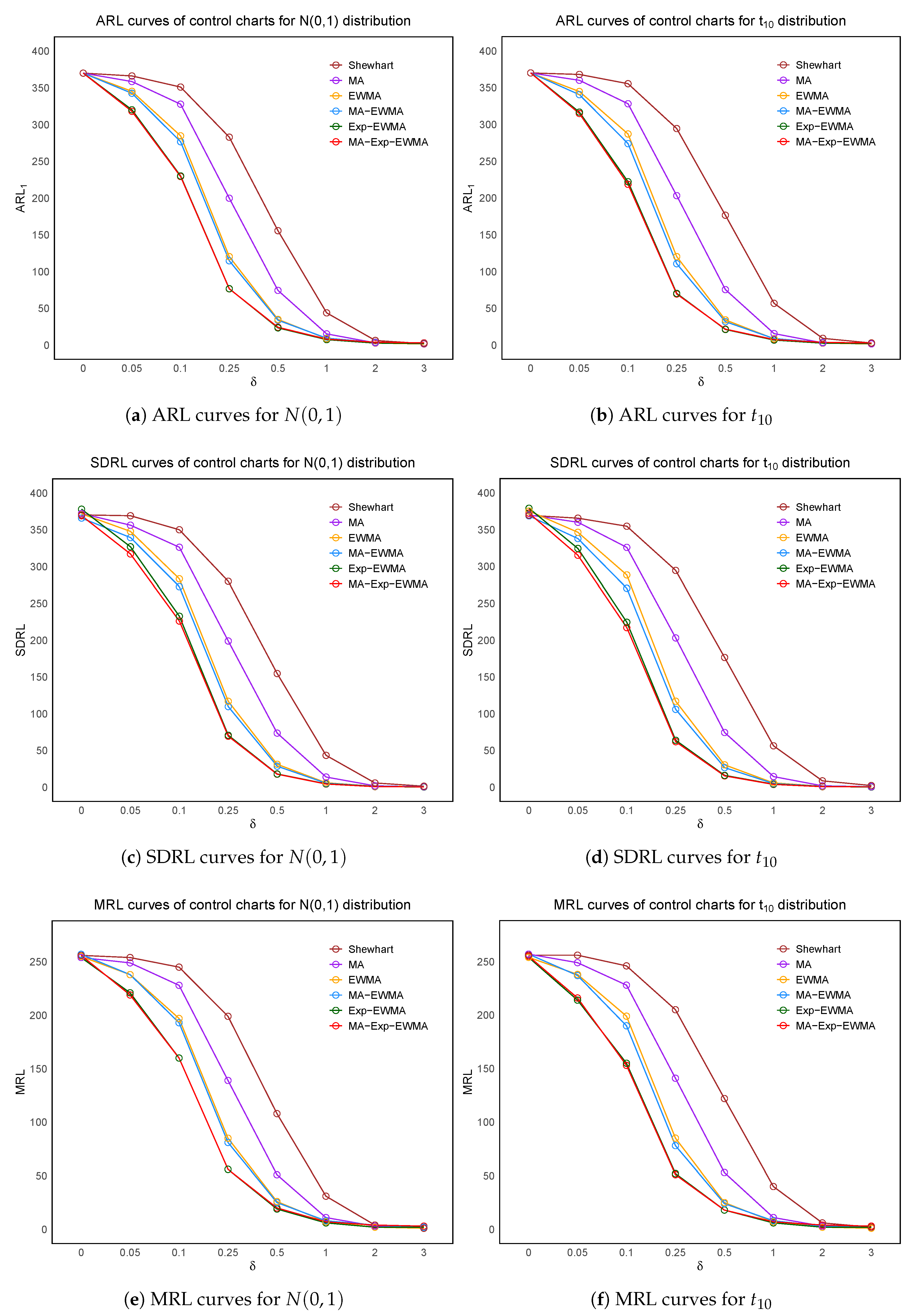
In this section, symmetric distributions are considered using the standard normal $N(0,1)$ and the $t_{10}$ distribution. The performance of various control charts is evaluated across different levels of shift $\left|\delta \right|$. Simulation results are summarized in

Table 13. Simulation result of $AR{L}_1$, SDRL, and $MRL$ for $N(0,1)$ distribution. The highlighted bold numbers represent the best results under the same shift.

	Shewhart			MA			EWMA			MA-EWMA			Exp-EWMA			MA-Exp-EWMA
Shift($\mathbf{\delta }$)	ARL	SDRL	MRL	ARL	SDRL	MRL	ARL	SDRL	MRL	ARL	SDRL	MRL	ARL	SDRL	MRL	ARL	SDRL	MRL
0.00	370.17	370.23	256	370.13	372.05	254	370.33	371.73	255	370.29	365.90	257	370.09	377.98	254	369.61	369.13	256
±0.05	366.20	369.08	254	358.56	356.22	249	345.26	347.79	238	342.64	339.37	238	320.11	326.82	221	318.09	317.08	219
±0.10	351.06	350.00	245	327.75	326.19	228	284.70	283.33	197	276.66	272.70	193	230.12	232.63	160	229.36	226.10	160
±0.25	282.89	279.98	199	199.82	198.96	139	120.39	116.92	85	114.70	109.69	81	76.74	70.70	56	76.57	69.42	56
±0.50	155.66	154.68	108	74.42	73.62	51	35.00	31.23	26	33.88	28.64	25	23.43	18.02	19	24.24	17.73	20
±1.00	43.87	43.36	31	15.28	13.86	11	8.80	6.09	7	9.41	5.47	8	7.43	4.63	6	8.15	4.34	7
±2.00	6.29	5.78	4	3.04	1.89	3	2.72	1.41	2	3.67	1.23	4	2.71	1.04	2	3.91	0.82	4
±3.00	2.00	1.41	1	1.58	0.70	1	1.53	0.67	1	2.34	0.74	2	2.06	0.26	2	3.06	0.52	3

and

Table 14. Simulation result of $AR{L}_1$, SDRL, and $MRL$ for $t_{10}$ distribution. The highlighted bold numbers represent the best results under the same shift.

	Shewhart			MA			EWMA			MA-EWMA			Exp-EWMA			MA-Exp-EWMA
Shift($\mathbf{\delta }$)	ARL	SDRL	MRL	ARL	SDRL	MRL	ARL	SDRL	MRL	ARL	SDRL	MRL	ARL	SDRL	MRL	ARL	SDRL	MRL
$0.00$	370.28	369.43	256.0	369.97	369.98	257.0	369.86	375.34	254.0	369.54	368.67	257.0	369.75	379.04	254.0	369.22	372.41	255.0
$\pm 0.05$	367.97	365.59	256.0	360.0	360.02	249.0	344.74	346.37	238.0	340.49	337.85	237.0	316.75	324.37	214.0	314.89	315.18	216.0
$\pm 0.10$	355.37	354.62	246.0	328.11	325.84	228.0	287.02	288.44	199.0	273.89	270.4	190.0	222.1	224.38	155.0	218.56	217.04	153.0
$\pm 0.25$	294.38	294.55	205.0	203.19	203.04	141.0	120.31	116.97	85.0	110.63	105.87	78.0	70.25	63.82	52.0	69.45	61.9	51.0
$\pm 0.50$	176.54	176.48	122.0	75.47	74.42	53.0	34.21	30.41	25.0	31.84	26.67	24.0	21.25	16.08	18.0	21.67	15.43	18.0
$\pm 1.00$	56.77	56.3	40.0	15.62	14.46	11.0	8.57	5.87	7.0	8.82	4.98	8.0	6.81	4.12	6.0	7.51	3.8	7.0
$\pm 2.00$	9.18	8.67	6.0	3.03	1.9	3.0	2.66	1.37	2.0	3.49	1.22	3.0	2.61	0.94	2.0	3.75	0.77	4.0
$\pm 3.00$	2.82	2.26	2.0	1.63	0.71	2.0	1.56	0.67	1.0	2.25	0.79	2.0	2.02	0.28	2.0	2.93	0.58	3.0

. These results are discussed below in terms of three key metrics: $AR{L}_1$, SDRL, and MRL.

From the results, under small shifts ($\left|\delta \right|\le 0.25$), the proposed MA-Exp-EWMA chart exhibits the best performance in both $AR{L}_1$ and SDRL, offering the shortest average detection time and the most stable variation. This advantage is consistent across both symmetric distributions, confirming its strength in early detection of small shifts.

For moderate shifts ($0.25<\left|\delta \right|\le 2$), MA-Exp-EWMA continues to lead in SDRL, indicating sustained stability. However, its $AR{L}_1$ becomes slightly less optimal than that of Exp-EWMA, suggesting that Exp-EWMA may detect medium shifts slightly faster. Still, MA-Exp-EWMA remains more stable overall.

When shifts are large ($\left|\delta \right|=3$), the EWMA control chart achieves the lowest $AR{L}_1$, indicating the fastest alarm, while Exp-EWMA exhibits the lowest SDRL, reflecting high detection stability. In this case, although MA-Exp-EWMA is slightly outperformed, it still demonstrates reasonable detection speed and excellent stability, making it a practical choice across the full range of shift magnitudes.

Regarding MRL, MA-Exp-EWMA often holds an advantage for small to moderate shifts, with only a slight drop under large shifts compared to some other methods. Overall, the MA-Exp-EWMA control chart shows strong and consistent performance under symmetric distributions, especially suited for early detection applications such as process monitoring. Its comprehensive performance is also visualized in Figure 1.

4.4.2. Exponential and Gamma Distributions

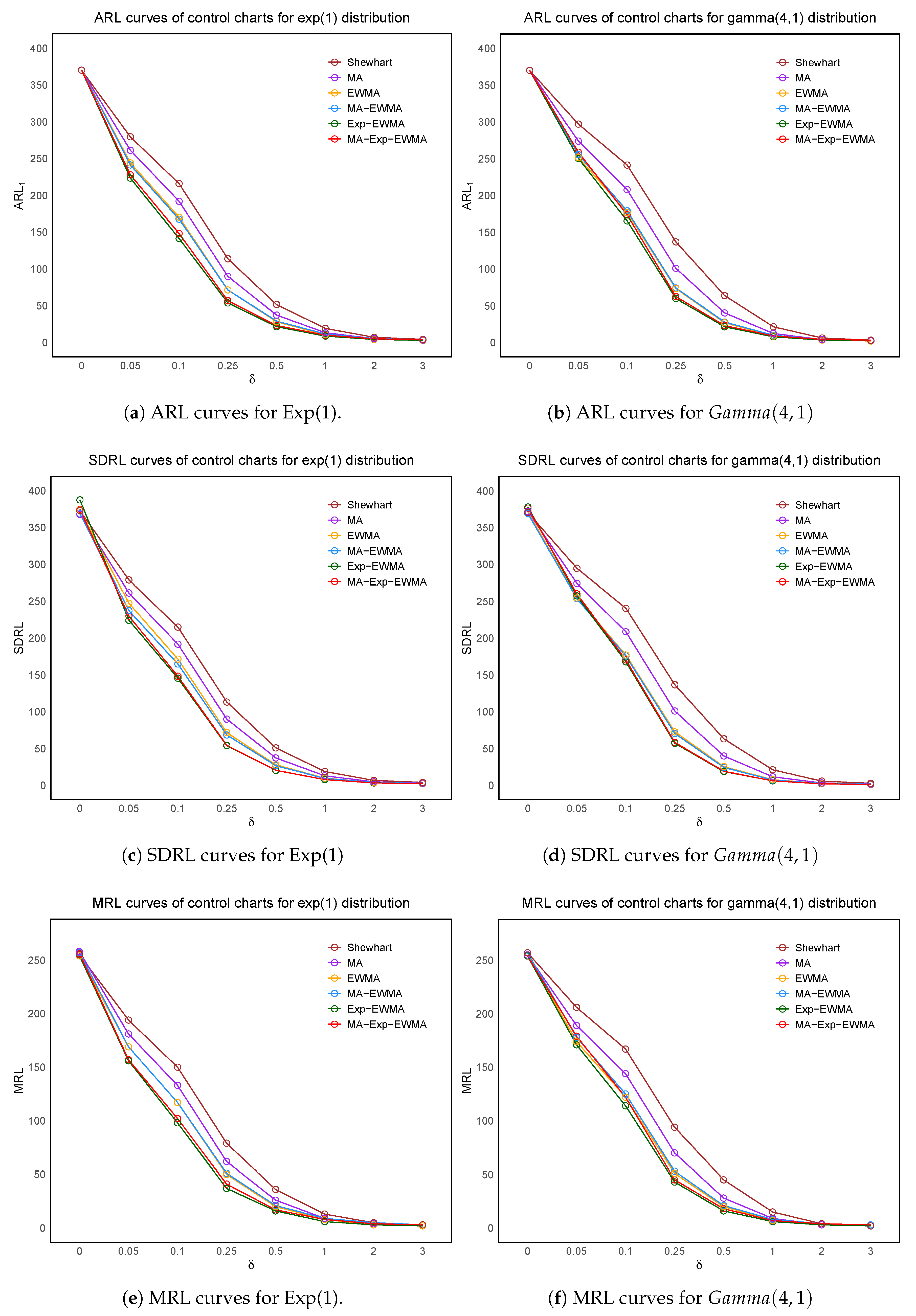
In this section, we analyze commonly encountered asymmetric distributions by evaluating the performance of control charts under the exponential distribution $Exp\left(1\right)$ and the gamma distribution $Gamma(4,1)$, across various shift magnitudes $\left|\delta \right|$. Simulation results are summarized in

Table 15. Simulation result of $AR{L}_1$, SDRL, and $MRL$ for $Exp\left(1\right)$ distribution. The highlighted bold numbers represent the best results under the same shift.

	Shewhart			MA			EWMA			MA-EWMA			Exp-EWMA			MA-Exp-EWMA
Shift($\mathbf{\delta }$)	ARL	SDRL	MRL	ARL	SDRL	MRL	ARL	SDRL	MRL	ARL	SDRL	MRL	ARL	SDRL	MRL	ARL	SDRL	MRL
$0.00$	369.96	372.84	255.0	369.97	367.74	258.0	369.89	373.63	254.0	370.0	368.59	257.0	370.3	387.46	245.0	370.57	374.45	256.0
$\pm 0.05$	279.5	278.78	194.0	261.24	261.25	181.0	244.07	247.38	169.0	241.31	237.34	169.0	223.41	224.28	156.0	227.91	229.9	157.0
$\pm 0.10$	215.85	214.94	150.0	191.93	191.75	133.0	170.34	171.5	117.0	167.64	164.86	117.0	141.37	145.53	98.0	148.04	148.19	102.0
$\pm 0.25$	113.86	113.14	79.0	89.93	89.85	62.0	71.5	71.63	50.0	71.49	68.39	51.0	53.83	53.86	37.0	56.83	54.24	41.0
$\pm 0.50$	51.57	50.86	36.0	37.31	37.22	26.0	28.24	27.83	20.0	29.14	26.69	21.0	21.56	20.36	16.0	23.2	20.43	17.0
$\pm 1.00$	19.25	18.76	13.0	13.36	12.88	9.0	10.53	9.68	8.0	11.56	9.36	9.0	8.77	7.71	6.0	9.99	7.7	8.0
$\pm 2.00$	7.16	6.68	5.0	5.31	4.74	4.0	4.58	3.9	3.0	5.41	3.9	5.0	4.2	3.31	3.0	5.13	3.22	4.0
$\pm 3.00$	4.38	3.85	3.0	3.43	2.86	3.0	3.09	2.47	2.0	3.74	2.6	3.0	2.99	2.06	2.0	3.82	2.13	3.0

and

Table 16. Simulation result of $AR{L}_1$, SDRL, and $MRL$ for $Gamma(4,1)$ distribution. The highlighted bold numbers represent the best results under the same shift.

	Shewhart			MA			EWMA			MA-EWMA			Exp-EWMA			MA-Exp-EWMA
Shift($\mathbf{\delta }$)	ARL	SDRL	MRL	ARL	SDRL	MRL	ARL	SDRL	MRL	ARL	SDRL	MRL	ARL	SDRL	MRL	ARL	SDRL	MRL
$0.00$	369.99	370.53	257.0	369.97	372.0	255.0	369.97	371.4	255.0	370.01	368.93	257.0	370.41	378.03	254.0	369.77	376.5	254.0
$\pm 0.05$	297.01	294.74	206.0	273.85	274.29	189.0	251.52	254.71	174.0	255.6	253.66	178.0	250.4	257.43	171.0	258.76	260.17	179.0
$\pm 0.10$	241.31	240.61	167.0	207.84	208.79	144.0	176.66	177.15	122.0	179.07	175.77	125.0	165.51	167.87	114.0	173.67	170.5	122.0
$\pm 0.25$	136.9	136.68	94.0	100.96	100.97	70.0	73.38	72.72	51.0	74.25	70.3	53.0	59.88	57.13	43.0	62.5	58.26	45.0
$\pm 0.50$	63.87	63.18	45.0	40.32	39.89	28.0	26.95	25.36	20.0	27.87	24.37	21.0	21.46	18.76	16.0	23.09	19.11	18.0
$\pm 1.00$	21.47	21.07	15.0	12.38	11.58	9.0	8.93	7.58	7.0	9.94	7.18	8.0	7.83	6.09	6.0	8.99	6.04	7.0
$\pm 2.00$	6.21	5.69	4.0	4.01	3.25	3.0	3.4	2.51	3.0	4.26	2.5	4.0	3.37	2.09	3.0	4.36	1.99	4.0
$\pm 3.00$	3.25	2.69	2.0	2.4	1.71	2.0	2.19	1.45	2.0	2.81	1.6	3.0	2.4	1.12	2.0	3.27	1.17	3.0

, and are discussed below using three key indicators—$AR{L}_1$, SDRL, and MRL.

Overall, across all shift levels, the Exp-EWMA control chart demonstrates the best performance in most scenarios in terms of $AR{L}_1$, SDRL, and MRL, indicating both fast and stable detection capabilities. The MA-Exp-EWMA control chart, in contrast, outperforms other methods in SDRL only at shift levels $\left|\delta \right|=1$ and $\left|\delta \right|=2$, suggesting that it provides relatively stable detection under moderate shift conditions.

Although MA-Exp-EWMA is not the top-performing method under very small or very large shifts—and generally lags in the MRL metric—it still maintains reasonable stability across most settings. In particular, it exhibits favorable performance under moderate shifts in asymmetric data. Thus, this method retains practical potential and application value when dealing with asymmetric data characterized by moderate shifts and stable variance. The overall results are illustrated in Figure 2.

4.4.3. Overview of Simulation Comparisons

Simulation results show that the proposed MA-Exp-EWMA control chart performs consistently well for symmetric distributions (e.g., normal and t), offering advantages in both detection speed ($AR{L}_1$) and stability (SDRL), indicating strong practical applicability.

For highly skewed distributions (e.g., exponential and gamma), the Exp-EWMA control chart generally achieves the best results, especially under large shifts. Although MA-Exp-EWMA excels in SDRL under moderate shifts, it performs less favorably in MRL and under extreme conditions.

In practice, real-world data often deviate from idealized distributions and rarely exhibit extreme skewness. The MA-Exp-EWMA control chart balances sensitivity and smoothness, enabling prompt response to early shifts and stable detection across a range of symmetric and moderately skewed data. Its superior SDRL further highlights robustness against variability.

Thus, excluding highly skewed scenarios, the MA-Exp-EWMA control chart is a flexible and reliable choice for applications requiring both accuracy and consistency.

5. Applications

This section analyzes two real-world datasets with time-evolving characteristics to verify the applicability and effectiveness of the proposed control chart methods. The parameter settings are fixed at $w=3,\lambda =0.2,a=0.75,c=0$, with the control limit L determined using Algorithm 1 in Section 4.1. These settings ensure an in-control average run length of approximately $AR{L}_0\approx 370$, enabling fair comparisons across all control charts.

Six control charts are applied: Shewhart, MA, EWMA, MA-EWMA, Exp-EWMA, and the proposed MA-Exp-EWMA. Their ability and timing in detecting shifts are compared to demonstrate the effectiveness of the proposed control chart.

This section proceeds by introducing the background and source of each dataset, explaining the monitoring objectives, and analyzing the data using all control chart methods. The shift detection times are then detailed, followed by a performance comparison to highlight the superior trend detection capability of the MA-Exp-EWMA control chart.

To align with the simulation phase and ensure comparability, all control charts adopt control limits L derived under the standard normal distribution $N(0,1)$. This choice is justified as the classical literature (e.g., Montgomery (2013) [17], Qiu (2014) [18]) confirms normal-based limits remain robust for data without strong skewness or heavy tails. Furthermore, deriving L individually introduces variability, undermining comparability, and studies (e.g., Ryan, (2011) [19]) show their continued effectiveness for slow shifts even with slight non-normality. Thus, normal-based control limits are adopted for fairness, robustness, and consistency.

5.1. Gold Price Analysis

Gold has long been regarded as an inflation-hedging and safe-haven asset, with prices influenced by global economic conditions and market sentiment, often fluctuating significantly during major events. For this study, monthly averages of gold spot prices in USD per ounce, covering the period from January 1978 to December 2024, were obtained from the World Gold Council’s Gold Spot Prices & Market History database (https://www.gold.org/goldhub/data/gold-prices, accessed on 4 May 2025). Over this period, the mean price was 779.9973, with a standard deviation of 576.1790. The dataset provides monthly, quarterly, and annual averages, with historical values available since 1978.

This time series exhibits stable periods followed by substantial volatility, making it suitable for testing the proposed control chart’s trend detection ability. To establish a stable reference, data from 1978 to 2007 were used as the baseline, as this period is relatively stable in terms of price movement. After 2007, however, the global economy experienced severe turbulence due to the 2008 financial crisis, leading to a surge in gold prices driven by increased demand for safe-haven assets. This structural shift provides a clear breakpoint for validating the trend detection capabilities of different control charts.

Figure 3 presents the results of applying six control charts—Shewhart, MA, EWMA, MA-EWMA, Exp-EWMA, and the proposed MA-Exp-EWMA—to the gold price data. Dates are shown in year.month format (e.g., 2024.03 = March 2024). These control charts signal the upward trend in gold prices at different time points: the Shewhart in March 2024, the MA in December 2010, the EWMA in September 2009, the MA-EWMA in July 2008, the Exp-EWMA in March 2008, and the proposed MA-Exp-EWMA detected the shift earliest in February 2008.

Figure 4 summarizes the results of all methods on the gold price data, clearly demonstrating the advantage of the MA-Exp-EWMA control chart in detecting trend shifts. Its ability to identify price deviations more quickly than other methods makes it valuable for early warning, financial risk management, and investment strategy adjustments.

5.2. GISS Surface Temperature Analysis

Changes in surface temperature are a key indicator of climate change, making trend monitoring critical as global warming gains attention. For this study, monthly global surface temperature anomaly data (land–ocean combined) from January 1951 to December 2024 were obtained from NASA’s Goddard Institute for Space Studies (GISS) GISTEMP version 4 (https://data.giss.nasa.gov/gistemp/, accessed on 4 May 2025). Over this period, the mean anomaly was 0.3394, with a standard deviation of 0.3775. The dataset is updated monthly and is based on multiple sources, including GHCN v4 for land stations and ERSST v5 for ocean regions. Values are expressed as deviations from the 1951–1980 baseline, with positive values indicating above-average and negative values indicating below-average temperatures.

The baseline period 1951–1980 is regarded as a relatively stable climatic phase. However, since the 1980s, anthropogenic greenhouse gas emissions have contributed to a systematic rise in global temperatures, leading to sustained warming, increased variability, and a greater frequency of extreme weather events. This long-term structural shift provides a suitable dataset for evaluating the performance of the proposed control chart in detecting gradual trends.

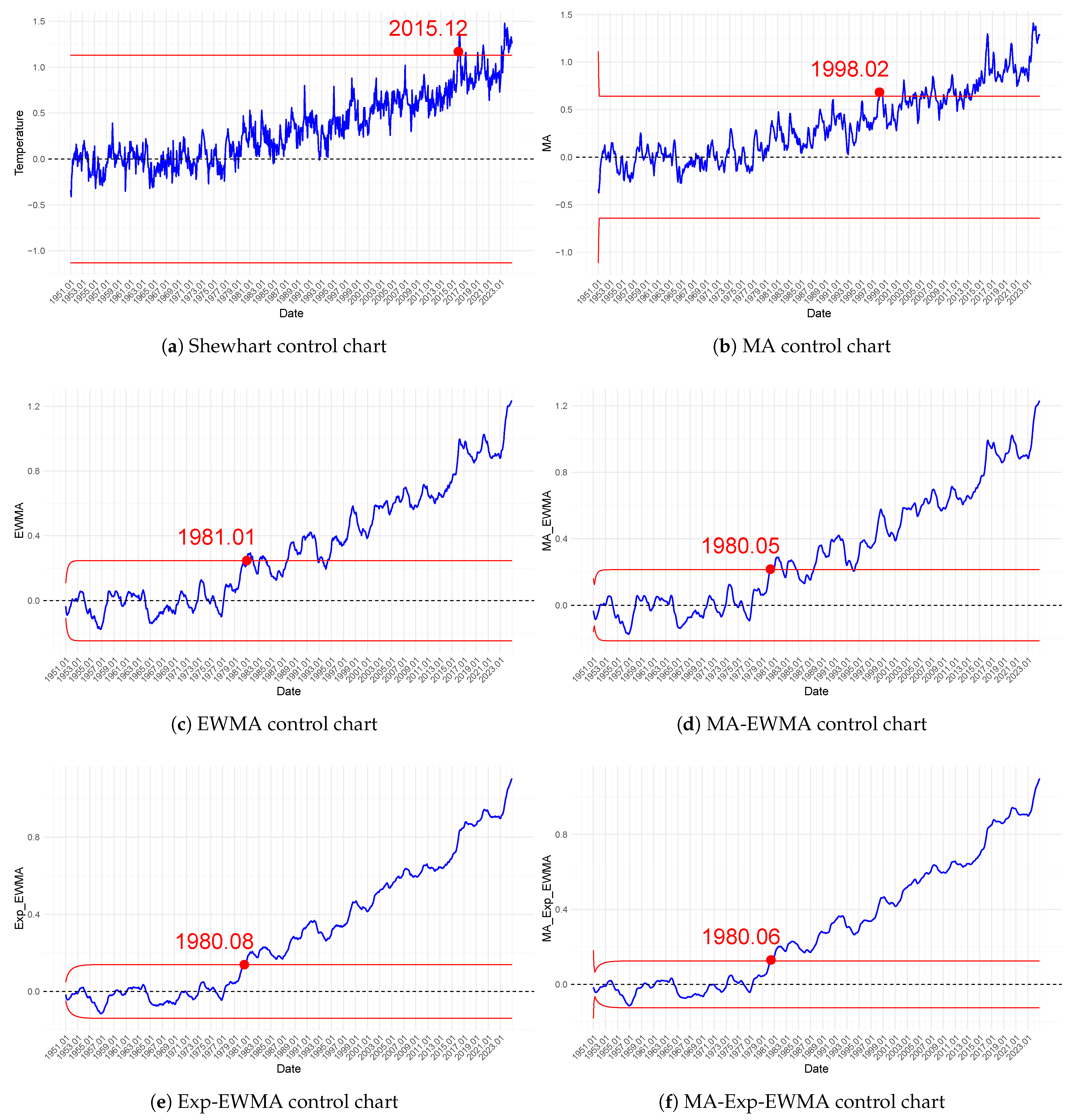
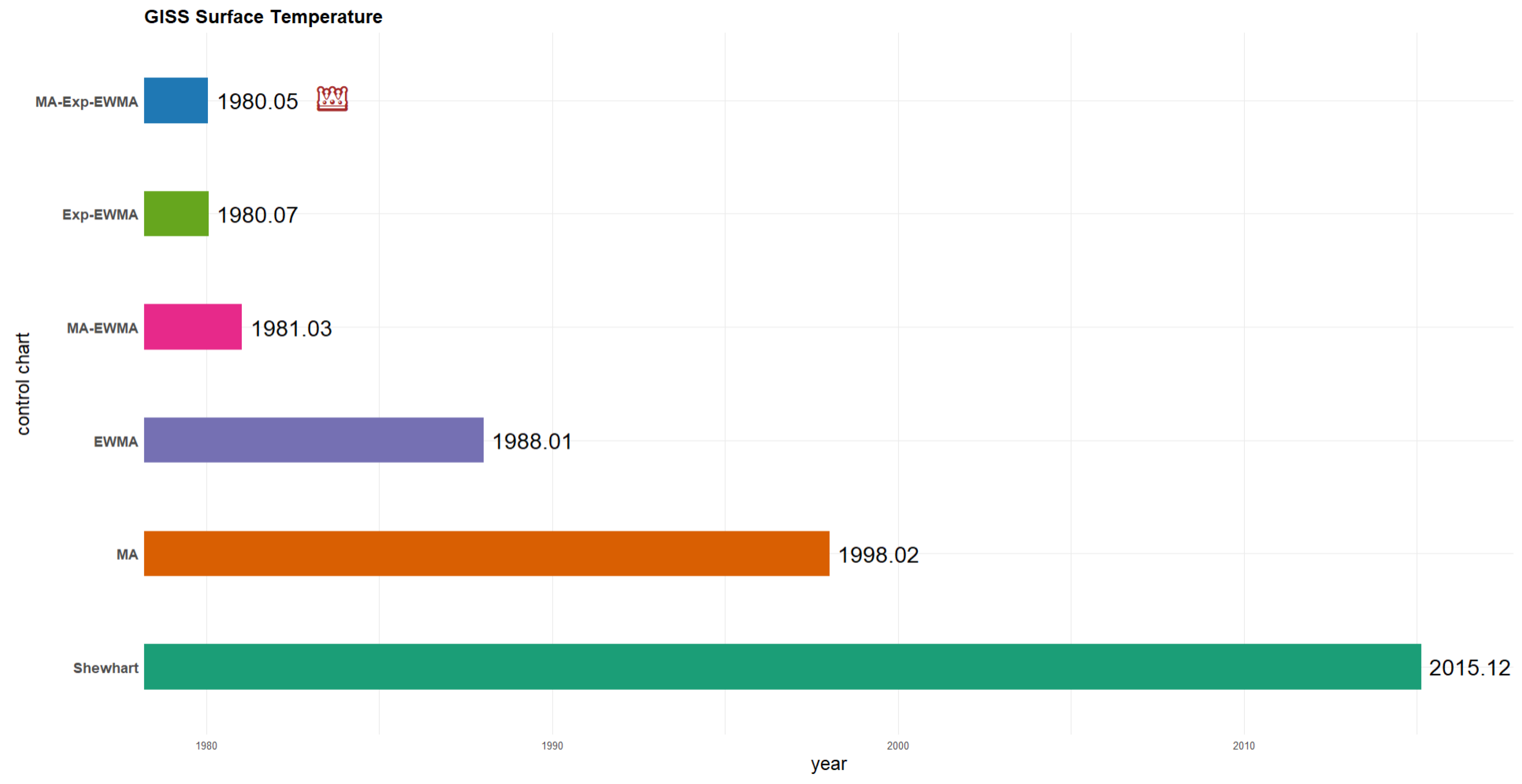
Figure 5 presents the results from six control charts applied to the GISS data: Shewhart, MA, EWMA, MA-EWMA, Exp-EWMA, and the proposed MA-Exp-EWMA. These control charts detected the upward trend in surface temperature at various time points: Shewhart in December 2015, MA in February 1998, EWMA in January 1988, MA-EWMA in March 1981, Exp-EWMA in July 1980, and MA-Exp-EWMA the earliest in May 1980.

Figure 6 summarizes the results, showing that MA-Exp-EWMA issued the earliest warning, highlighting its superior sensitivity and responsiveness. This suggests that, for time series like surface temperature—marked by a long-term stable baseline followed by gradual change—MA-Exp-EWMA is a more efficient and powerful tool. It enables early detection of trend shifts and enhances the timeliness and foresight of climate risk management.

6. Conclusions

In the current data-driven industrial environment, the timeliness and sensitivity of quality monitoring methods are increasingly important. Although traditional control charts are effective in managing stable processes, they often face limitations in detection efficiency and robustness when identifying trending variations or small shifts. Therefore, the development of a control chart that achieves both rapid responsiveness and false alarm control has become a crucial issue in the field of statistical process monitoring.

This study introduces a novel control chart—the MA-Exp-EWMA control chart—constru- cted based on the frameworks of MA-EWMA and Exp-EWMA control charts. It integrates the smoothing property of the MA and the time-varying weighting mechanism of the exponentially weighted approach, aiming to balance stability and sensitivity. Simulation results indicate that the proposed method performs well under symmetric and moderately skewed distributions, offering advantages in terms of detection speed ($AR{L}_1$) and stability (SDRL). Although its performance under extremely skewed distributions is slightly lower than that of the Exp-EWMA control chart, the overall results remain competitive. This method is especially suitable for monitoring processes with nearly symmetric distributions and small magnitude shifts.

In addition, real-world applications further confirm the practical effectiveness of the proposed method. In time series data such as gold prices and global surface temperatures, which exhibit trending variation, the MA-Exp-EWMA control chart is able to signal process shifts earlier than other methods, demonstrating high sensitivity and prompt detection capability.

The proposed MA-Exp-EWMA chart advances control chart design in several important ways. First, by integrating a Moving Average with exponential smoothing, it overcomes the limitations of static weighting and fixed smoothing methods, offering a more adaptive approach. Second, this hybrid structure enhances responsiveness not only to gradual shifts but also to sudden changes, while retaining robustness when applied to non-standard data structures such as autocorrelated or non-normal processes. Third, the chart provides improved timeliness and accuracy in process quality monitoring, which is especially beneficial in critical or variable environments where early and reliable detection is essential. Together, these features extend the theoretical foundations of hybrid control charts and represent a step forward in practical monitoring applications, thereby positioning the MA-Exp-EWMA as an innovative contribution beyond a simple methodological extension.

Our proposed MA-Exp-EWMA chart contributes to this line of research by integrating the advantages of MA and Exp-EWMA. Similar to recent innovations such as the Tukey-modified EWMA–MA chart (Talordphop et al., 2022) [16], the extended EWMA chart (Karoon et al., 2025 [20]), the EWMA-DMA chart (Taboran and Sukparungsee, 2023 [21]), and the exponentiated EWMA chart (Alevizakos et al., 2024 [12]), our approach highlights the ongoing evolution of control chart designs aimed at improving small-shift detection.

To summarize, the MA-Exp-EWMA control chart demonstrates consistent performance in simulation studies and provides early warning capability in practical applications. It is expected to be widely applicable to various tasks involving variation monitoring and trend detection, and serves as an important statistical tool that combines robustness and sensitivity.

References

1. Shewhart, W.A. Economic Control of Quality of Manufactured Product; D. Van Nostrand Company, Inc.: New York, NY, USA, 1931. [Google Scholar]
2. Shewhart, W.A. Statistical Method from the Viewpoint of Quality Control; The Graduate School, The Department of Agriculture: Washington, DC, USA, 1939. [Google Scholar]
3. Page, E.S. Cumulative sum charts. Technometrics 1961, 3, 1–9. [Google Scholar] [CrossRef]
4. Roberts, S.W. A comparison of some control chart procedures. Technometrics 1970, 12, 717–732. [Google Scholar] [CrossRef]
5. Xie, M.; Goh, T.N.; Ranjan, P. Some effective control chart procedures for monitoring process mean and variability. Int. J. Prod. Res. 2000, 38, 3971–3986. [Google Scholar]
6. Paichit, P.; Peerajit, W. The average run length for continuous distribution process mean shift detection on a modified EWMA control chart. Asia-Pac. J. Sci. Technol. 2022, 27, 1–13. [Google Scholar]
7. Talordphop, K.; Areepong, Y.; Sukparungsee, S. An empirical assessment of Tukey combined extended exponentially weighted moving average control chart. AIMS Math. 2025, 10, 3945–3960. [Google Scholar] [CrossRef]
8. Makaew, S.; Areepong, Y.; Sukparungsee, S. Average Run Length in TEWMA Control Charts: Analytical Solutions for AR (p) Processes and Real Data Applications. Comput. Model. Eng. Sci. 2025, 143, 1617–1634. [Google Scholar] [CrossRef]
9. Roberts, S.W. Control chart tests based on geometric moving averages. Technometrics 1959, 1, 239–250. [Google Scholar] [CrossRef]
10. Khoo, M.B. A moving average control chart for monitoring the fraction non-conforming. Qual. Reliab. Eng. Int. 2004, 20, 617–635. [Google Scholar] [CrossRef]
11. Taboran, R.; Sukparungsee, S.; Areepong, Y. Mixed moving average-exponentially weighted moving average control charts for monitoring of parameter change. In Proceeding of the International MultiConference of Engineers and Computer Scientists, Hong Kong, China, 13–15 March 2019; pp. 13–15. [Google Scholar]
12. Alevizakos, V.; Chatterjee, A.; Chatterjee, K.; Koukouvinos, C. The exponentiated exponentially weighted moving average control chart. Stat. Pap. 2024, 65, 3853–3891. [Google Scholar] [CrossRef]
13. Duncan, A.J. Quality Control and Industrial Statistics, 5th ed.; Irwin: Homewood, IL, USA, 1986. [Google Scholar]
14. Tang, T.-H. A Study on the Ma-Gwma Control Chart for Detecting Small Shifts. Master’s Thesis, National Chung Hsing University, Taichung, Taiwan, 2024. [Google Scholar]
15. Zou, C.; Tsung, F. A multivariate sign ewma control chart. Technometrics 2011, 53, 362–375. [Google Scholar] [CrossRef]
16. Talordphop, K.; Sukparungsee, S.; Areepong, Y. Performance of new nonparametric Tukey modified exponentially weighted moving average—Moving average control chart. PLoS ONE 2022, 17, e0275260. [Google Scholar] [CrossRef]
17. Montgomery, D.C. Introduction to Statistical Quality Control, 7th ed.; Wiley: Hoboken, NJ, USA, 2013. [Google Scholar]
18. Qiu, P. Introduction to Statistical Process Control; Chapman and Hall/CRC: Boca Raton, FL, USA, 2014. [Google Scholar]
19. Ryan, T.P. Statistical Methods for Quality Improvement, 3rd ed.; Wiley: Hoboken, NJ, USA, 2011; pp. 291–305. [Google Scholar]
20. Karoon, K.; Areepong, Y. The efficiency of the new extended EWMA control chart for detecting changes under an autoregressive model and its application. Symmetry 2025, 17, 104. [Google Scholar] [CrossRef]
21. Taboran, R.; Sukparungsee, S. On designing of a new EWMA-DMA control chart for detecting mean shifts and its application. Thail. Stat. 2023, 21, 148–164. [Google Scholar]
Figure 1. Control chart performance—symmetric.
Mathematics 13 03049 g001
Figure 2. Control chart performance—skew.
Mathematics 13 03049 g002
Figure 3. Results of gold price analysis using different control charts.
Mathematics 13 03049 g003
Figure 4. Comparison of control chart results for gold price analysis.
Mathematics 13 03049 g004
Figure 5. Result of GISS surface temperature analysis.
Mathematics 13 03049 g005
Figure 6. Comparison of control chart results for GISS surface temperature analysis.
Mathematics 13 03049 g006