Abstract
Nonlinear complex systems exhibit emergent behavior, sensitivity to initial conditions, and rich dynamics arising from interactions among their components. A classical example of such a system is the Troesch problem—a nonlinear boundary value problem with wide applications in physics and engineering. In this work, we investigate and compare two distinct approaches to solving this problem: the Differential Transform Method (DTM), representing an analytical–symbolic technique, and Physics-Informed Neural Networks (PINNs), a neural computation framework inspired by physical system dynamics. The DTM yields a continuous form of the approximate solution, enabling detailed analysis of the system’s dynamics and error control, whereas PINNs, once trained, offer flexible estimation at any point in the domain, embedding the physical model into an adaptive learning process. We evaluate both methods in terms of accuracy, stability, and computational efficiency, with particular focus on their ability to capture key features of nonlinear complex systems. The results demonstrate the potential of combining symbolic and neural approaches in studying emergent dynamics in nonlinear systems.
Keywords:
physical-informed neural network; differential transform method; Troesch problem; nonlinear dynamics; boundary value problems MSC:
34; 65; 65L10; 68; 68T07; 68T20
1. Introduction
Troesch’s problem is closely related to mass and heat transfer phenomena. It serves as a benchmark model for challenging nonlinear differential equations, analogous to those encountered in continuum physics. Specifically, Troesch’s problem models transport through semipermeable membranes, diffusion with reactivity, or nonlinear behaviors in conductive processes—such as in plasma reactors or biological membranes.
It arises in contexts involving a balance between nonlinear diffusion and reaction, typically under Dirichlet boundary conditions. The nonlinearity may stem from equations describing electric field penetration, temperature gradients, or chemical concentration differences. In physical applications, the problem can represent diffusion models in semiconductors, heat conduction with nonlinear temperature dependence, mass transport through reactive biological membranes, or electric field modeling in plasmas.
In recent decades, there has been an intensive development of analytical methods for solving ordinary differential equations (ODEs) and partial differential equations (PDEs), particularly in the context of nonlinear models. One of the effective and widely used techniques in this area is the Differential Transform Method (DTM)—an analytical method based on series transformations (most commonly the Maclaurin series). Unlike methods such as the Homotopy Perturbation Method (HPM) [1,2] or the Adomian Decomposition Method [3,4], the DTM does not require prior linearization or discretization of equations. As a result, it is naturally suited for solving complex, strongly nonlinear problems or those difficult to address numerically. The DTM can be applied to the analysis of equations and systems of operator equations, including but not limited to ordinary differential equations, partial differential equations, integral equations or their systems [5,6,7], dynamic systems modeling physical, biological, and engineering processes, and boundary and initial value problems [7,8].
The DTM allows us to transform a given problem into a system of recurrence equations for the coefficients of a power series. This approach enables us to obtain analytical solutions that maintain the continuity and differentiability of the approximate solution. Often, just a few initial terms of the expansion yield high-quality approximations, which makes the DTM computationally efficient. In many cases, the method even allows us to find the exact solution. An additional advantage of the method is its relatively simple implementation in computer-aided symbolic computation environments, such as the Mathematica computational platform used in this work, which has a wide range of applicability in various engineering problems [9,10,11].
In recent years, machine learning-based techniques have been playing an increasingly important role in computer simulations and mathematical modeling. One possible approach is the use of neural networks to solve initial boundary value problems. An example of such networks are Physics-Informed Neural Networks (PINNs). The advantages of this type of approach include mesh independence, low requirements for mathematical transformations, and the ability—once the model is trained—to instantly obtain results for any points in the domain without the need for recomputation. Some of the earliest and most important works in this field are the papers by Raissi [12,13,14,15]. These works describe PINNs in the context of solving forward and inverse problems of differential equations. They present the idea behind using neural networks in this way. The authors of [13] focus on a review of PINNs, various variants of such networks, and their applications to different types of problems and outline different directions of development. It is worth mentioning several works where PINNs have been applied in various domains. For example, ref. [16] presents the use of PINNs for modeling biological and epidemiological dynamical systems. The authors consider a system of ordinary differential equations and seek an inverse solution involving parameter estimation of the model. Another interesting article is [17], in which the authors use PINN-type neural networks for predicting 3D soft tissue dynamics from 2D imaging. An example of using PINNs in engineering problems is the paper [18], which considers the heat transfer equation. The predictions of the trained PINN were validated in several 1D and 2D heat transfer cases by comparison with FE results. It was shown that both a standard neural network (NN) and a PINN accurately reproduced the results of the finite element method during training. However, only the PINN with appropriately selected features was able to grasp the physical principles governing the problem and predict correct results even outside the range of the training data. More information on the applications of PINNs can be found in the articles [19,20,21,22].
In this paper, we focus on solving the Troesch problem. To this end, we use two fundamentally different methods: the DTM and PINNs. Section 2 describes the problem to be solved—a second-order ordinary differential equation. Section 3 and Section 4 are devoted to the descriptions of both methods—the DTM first, followed by PINNs. These sections present the main ideas behind each method. Section 5 describes the results obtained for the Troesch problem using the DTM and PINNs. A comparison of both methods is also provided. Finally, Section 6 presents the conclusions drawn from the research.
2. Problem Statement
In this study, we consider a boundary value problem defined by the following equation along with its associated conditions:
where . The above equation is known as the Troesch problem. Due to its strong nonlinearity, this problem is particularly challenging to solve numerically, especially when . A distinctive feature of this equation is the rapid increase in nonlinearity as the parameter increases, which leads to numerical difficulties. In particular, the solution becomes increasingly steep as x approaches 1. The high stiffness of this differential equation can make many standard numerical methods unstable. For methods based on domain discretization, extremely fine meshes may be required to obtain reliable results.
The Troesch equation arises in the context of modeling various physical phenomena, including the study of plasma confinement under radiation pressure [23,24], as well as in the analysis of transport processes in gas-porous electrodes [25,26,27].
3. The DTM in Practice: Solving a Stiff Nonlinear Equation
In this work a function f that can be expanded into a Taylor series around a fixed point is referred to as the original. A special case of this expansion is the Maclaurin series, which arises when . In the following discussion, we will focus exclusively on functions that meet the conditions of being originals in the above sense and will make use of the Maclaurin series.
In the adopted context, the notion of a Taylor series is understood in a broader sense than in traditional definitions. Assuming that the function f is an original, it is possible to express the variable mapping in the form
which—under the assumption of a unique expansion—allows us to associate with each original a unique transformation in the form of a function :
As a result, a function that is an original can be written as
In the process of solving a given mathematical problem, it is often possible to use known expansions of elementary functions as well as the properties of the transformation itself, which reduces the problem to purely algebraic operations. Although the literature on the Differential Transform Method (DTM) describes a broad range of its properties, in this work, we will limit ourselves to presenting only those necessary for solving the problem under consideration. In what follows, we assume that the variable x belongs to the domain of the function f, which satisfies the conditions required for an original.
Property 1.
If the function f is of the form , then
Property 2.
If the function f is of the form , then
Property 3.
If the function f is of the form , , then
Property 4.
If the function f is of the form , , , then
4. Application of PINNs to a Stiff Boundary Problem
Neural networks have for several years been a powerful tool for solving a wide range of problems, such as image analysis, speech recognition, and others. The PINN-type network is designed to address forward and inverse problems based on various types of equations, including differential, integral, and integro-differential equations [7,28,29,30,31]. The use of neural networks for this class of problems is a relatively recent approach and fundamentally different from classical numerical methods.
The core idea behind Physics-Informed Neural Networks (PINNs) is the integration of physical laws into the deep learning model training process. During model training, the loss function incorporates the underlying physics, i.e., the governing equations along with the corresponding initial and boundary conditions. Unlike many traditional numerical methods, the PINN approach does not require meshing or domain discretization. This is made possible through a computational technique known as automatic differentiation, which enables the accurate computation of derivatives of composite functions based on elementary mathematical operations and the chain rule.
The structure of a PINN-type network typically consists of two essential components: a neural network (most commonly a fully connected feedforward network) and a physics-informed loss function. The loss function accounts for the approximation errors of the differential equation solution, initial and boundary conditions, and any additional data (e.g., measurements required for solving an inverse problem). A general schematic of a PINN architecture for forward problems is presented in Figure 1.
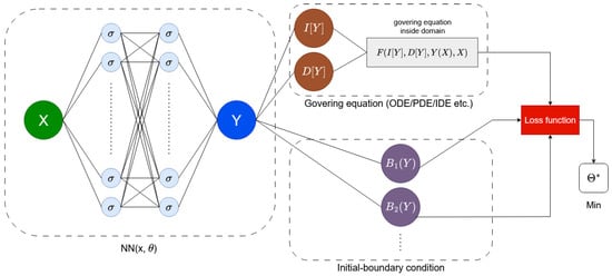
Figure 1.
PINN-type scheme for forward problems.
The input to the neural network (denoted as X in Figure 1) consists of the coordinates of points from the domain of the equation, while the network’s output represents the approximate value of the solution at the given points (denoted as Y in the figure). The diagram also illustrates blocks corresponding to the governing equation and the initial boundary conditions. The symbols I, D, and F denote, respectively, the integral operator, the differential operator, and the function defining the equation.
In the case of inverse problems (not shown in the diagram), additional data may also be considered (e.g., observations or measurements). The loss function accounts for the approximation errors of the equation and the initial boundary conditions:
where denotes the approximation errors within the domain, corresponds to the errors associated with the initial and boundary conditions, and , are the weighting coefficients.
For the Troesch problem, we adopted a loss function composed solely of the approximation errors within the domain:
where M denotes the number of training (or collocation) points randomly sampled from the domain. In this case, the operator F is defined as follows:
For the boundary conditions, we applied a technique known as a hard boundary condition. This involves embedding the boundary conditions directly into the structure of the trial solution instead of imposing them softly by adding a penalty term to the loss function. In practice, this is performed by transforming the output of the neural network through a function that enforces the boundary conditions. In the considered case, this function takes the form
where denotes the output of the neural network with parameters . The function denotes the approximation of the solution, obtained from the output of the neural network and constructed to exactly satisfy the boundary conditions. It is easy to verify that this construction satisfies the boundary conditions exactly: and . As a result, the boundary conditions are satisfied exactly rather than approximately during the model training. Furthermore, this approach accelerates the learning process. It is also worth noting that the PINN framework focuses on training a model. Once the model is trained, it can provide the unknown function values at any point in the domain without the need to recompute the solution. In contrast, classical grid-based numerical methods require recomputation whenever the grid is changed.
5. Results and Discussion
In this section, we compare the solutions to the Troesch problem obtained using two different methods: the DTM and PINNs. The former allows obtaining the solution in the form of a continuous function. The latter, namely PINNs, is a relatively new approach in which information about the differential equation is incorporated into the training of the neural network, and the results are obtained in a discrete form.
5.1. Results Obtained from DTM
In order to decompose the problem (1) into algebraic dependencies, we use the relations (2)–(5), whereby the equation in question is rewritten, for the purpose of the solution, in the form , where
with , . For , we then obtain
and since from the condition we have , it follows from Equation (10), knowing that , that . Unfortunately, we do not know the value of (since the boundary conditions of problem (1) do not include a condition for ), and so, for the purpose of the solution, we introduce a temporary assumption , where is an unknown constant.
For example, for we obtain
and hence ; for we obtain
and thus ; for we obtain
and hence
Therefore, if we aim to construct a degree-5 polynomial that serves as an approximate solution to problem (1), we obtain
in which the unknown parameter s appears. The value of this parameter will be determined for a fixed value of , using the boundary condition , i.e., by solving the equation with respect to the unknown s. In this case (with ), the parameter s takes the value , and the polynomial takes the form
We now compare the solution values obtained using the DTM with the exact values of for . The predicted values for are summarized in Table 1, Table 2 and Table 3. For , the DTM solutions show excellent agreement with the exact values, with very small errors observed throughout the domain, even for lower-order approximations. The accuracy remains high for , with deviations decreasing steadily as n increases. In the more nonlinear case of , the errors become more pronounced, especially as the value of x increases. For instance, at , the error at reaches approximately 0.263, corresponding to a relative error of about 172.78%. This highlights the slower convergence rate of the DTM in highly nonlinear regimes. Nevertheless, the method still captures the overall behavior of the solution well, and accuracy improves significantly with increasing n, particularly for smaller values of x.

Table 1.
Solution values obtained using DTM for compared with exact values .
Table 2.
Solution values obtained using DTM for compared with exact values .
Table 3.
Solution values obtained using DTM for compared with exact values .
The error graphs shown in Figure 2, Figure 3 and Figure 4 reveal distinct patterns in how the accuracy of the DTM evolves with both the degree of nonlinearity and the position within the domain. For all values of , errors are minimal near and increase monotonically with x, highlighting that the method performs best close to the initial point and gradually loses precision towards . This growth in error with respect to x becomes more pronounced as increases. In the linear case (), errors remain uniformly low and change slowly across x, while for , the increase is more noticeable but still controlled. In contrast, for , the rate of error escalation with x is steep, with a relatively sharp increase beyond , indicating a strong sensitivity to domain position under high nonlinearity. Furthermore, while increasing n reduces error at all x, the improvement is more significant in regions with smaller x, suggesting that the DTM converges more rapidly in the early part of the domain and struggles to maintain accuracy near the boundary in nonlinear cases. This increase in error across the domain shows a key weakness of the DTM in nonlinear problems and suggests that using higher-order approximations may be necessary to maintain consistent accuracy.
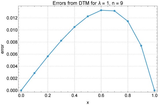
Figure 2.
DTM method errors for and .
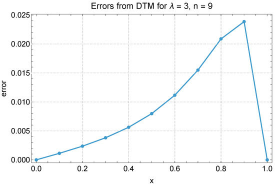
Figure 3.
DTM method errors for and .
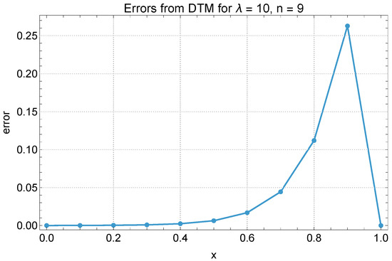
Figure 4.
DTM method errors for and .
5.2. Results Obtained from PINN
At the outset, it should be emphasized that the Troesch problem considered in this study is known for its strong nonlinearity and stiffness, particularly for large values of (), which makes it challenging to solve using classical methods as well as Physics-Informed Neural Networks (PINNs).
After a preliminary analysis of the model’s hyperparameters, the following configuration was established:
- The neural network consisted of three hidden layers, each containing 10 neurons;
- The training was performed using the Adam optimizer with a learning rate of ;
- The number of training points was set to 50.
Figure 5 presents solutions obtained with PINNs for different values of the parameter . The larger the value of the parameter , the more nonlinear the solution becomes, and the inflection point of the curve is closer to . Higher values of also make Equation (1) more difficult to solve.
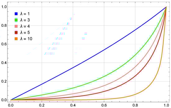
Figure 5.
Solutions obtained using PINN for different values of .
We now compare the solution values obtained using PINNs with the exact values taken from the paper [4] for . The results of this comparison can be found in Table 4 and Table 5. Figure 6, Figure 7 and Figure 8 show the error distribution over the entire domain for . In each case, the errors were small, with particularly good results obtained for the case . In the most computationally challenging case (), the approximation results are also very good, with errors not exceeding . From the error distribution plots, it can also be observed that the maximum errors occurred for x close to the inflection point; e.g., in the case of , the maximum error is reached at approximately .
Table 4.
Comparison of exact values of and PINN approximations for and .
Table 5.
Comparison of exact values of and PINN approximations for .
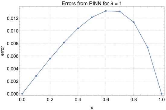
Figure 6.
PINN method errors for .
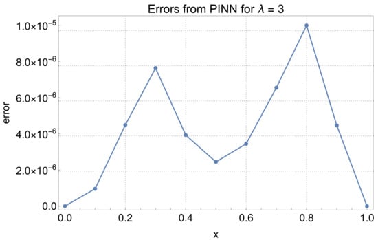
Figure 7.
PINN method errors for .
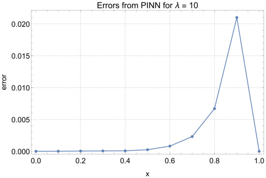
Figure 8.
PINN method errors for .
5.3. DTM vs. PINN Results Comparison
A direct comparison between the results obtained using the DTM and PINN methods for reveals notable differences in performance, especially as the degree of nonlinearity increases. For the linear case (), both methods yield almost identical results, with very small and evenly distributed errors across the domain. This indicates that both approaches are equally effective in handling linear problems. For , the accuracy of PINNs remains consistently high, with error values remaining below throughout the domain. In contrast, DTM errors begin to increase more noticeably with increasing x, although the method still captures the solution trend reasonably well. The distinction becomes even more pronounced for , where the PINNs continue to produce accurate approximations, with the maximum error staying below 0.021. Meanwhile, the DTM solution exhibits a significant increase in error, especially in the latter half of the domain, reaching 0.263 at . This indicates a decline in the DTM’s effectiveness under strong nonlinearity, unless much higher-order expansions are used. Overall, PINNs demonstrate superior stability and accuracy across all situations, particularly excelling in highly nonlinear scenarios where the DTM struggles to maintain precision without increasing computational cost (Figure 9, Figure 10 and Figure 11).
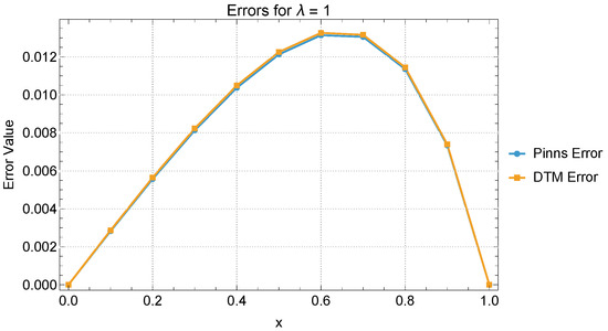
Figure 9.
PINN and DTM error comparison for .
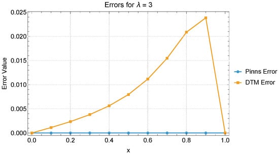
Figure 10.
PINN and DTM error comparison for .
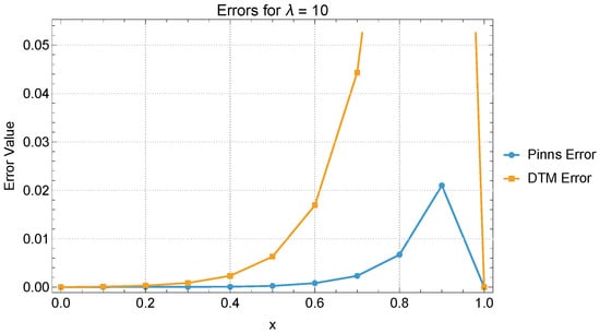
Figure 11.
PINN and DTM error comparison for .
6. Conclusions
This work focuses on presenting two different numerical methods: PINNs (Physics-Informed Neural Networks) and the DTM (Differential Transform Method). These methods were used to solve the Troesch problem, which consists of a nonlinear differential equation with boundary conditions. The approaches described in this paper are completely different. In the case of the DTM, the solution is obtained in the form of a polynomial, while the PINN method is based on neural networks and provides results in a discrete form. This article demonstrates the effectiveness of both methods. A comparison of the results showed that both methods perform well for small values of the parameter , but for larger values, the PINN method performs significantly better.
For , both methods produced very accurate and similar results. At , PINNs still maintained high accuracy, while the DTM began to show increasing errors in the second half of the domain. The biggest differences appear for , where PINNs preserved good precision and the DTM returned large errors, especially towards the end of the domain. It can therefore be concluded that PINNs are a more stable and accurate method, especially for strongly nonlinear problems, where the DTM requires much higher computational effort to achieve similar accuracy.
Author Contributions
Conceptualization, R.B., M.P., J.B. and M.C.; methodology, J.B., M.C., C.N. and G.C.; software, R.B., M.P., J.B. and M.C.; validation, C.N. and G.C.; investigation, R.B., M.P., J.B., M.C., C.N. and G.C.; writing—original draft preparation, R.B., J.B. and M.C.; writing—review and editing, R.B., J.B. and M.C. All authors have read and agreed to the published version of the manuscript.
Funding
This research received no external funding.
Institutional Review Board Statement
Not applicable.
Informed Consent Statement
Not applicable.
Data Availability Statement
The datasets generated and/or analyzed during the current study are available from the corresponding author upon reasonable request.
Conflicts of Interest
The authors declare no conflicts of interest. The funders had no role in the design of the study; in the collection, analyses, or interpretation of data; in the writing of the manuscript; or in the decision to publish the results.
References
- Grzymkowski, R.; Hetmaniok, E.; Slota, D. Application of the homotopy perturbation method for calculation of the temperature distribution in the cast-mould heterogeneous domain. J. Achiev. Mater. Manuf. Eng. 2010, 43, 299. [Google Scholar]
- He, J.H. An elementary introduction to the homotopy perturbation method. Comput. Math. Appl. 2009, 57, 410–412. [Google Scholar] [CrossRef]
- Adomian, G. Solving Frontier Problems of Physics: The Decomposition Method; Springer Science & Business Media: Berlin/Heidelberg, Germany, 2013; Volume 60. [Google Scholar]
- Pleszczyński, M.; Kaczmarek, K.; Słota, D. Application of a Hybrid of the Different Transform Method and Adomian Decomposition Method Algorithms to Solve the Troesch Problem. Mathematics 2024, 12, 3858. [Google Scholar] [CrossRef]
- Abazari, R.; Ganji, M. Extended two-dimensional DTM and its application on nonlinear PDEs with proportional delay. Int. J. Comput. Math. 2011, 88, 1749–1762. [Google Scholar] [CrossRef]
- Brociek, R.; Pleszczyński, M. Comparison of selected numerical methods for solving integro-differential equations with the Cauchy kernel. Symmetry 2024, 16, 233. [Google Scholar] [CrossRef]
- Brociek, R.; Pleszczyński, M. Differential Transform Method (DTM) and Physics-Informed Neural Networks (PINNs) in Solving Integral–Algebraic Equation Systems. Symmetry 2024, 16, 1619. [Google Scholar] [CrossRef]
- Abazari, R.; Abazari, M. Numerical simulation of generalized Hirota–Satsuma coupled KdV equation by RDTM and comparison with DTM. Commun. Nonlinear Sci. Numer. Simul. 2012, 17, 619–629. [Google Scholar] [CrossRef]
- Lynch, S. Dynamical Systems with Applications Using Mathematica; Springer: Berlin/Heidelberg, Germany, 2007. [Google Scholar]
- Sitek, G.; Pleszczyński, M. Inferring About the Average Value of Audit Errors from Sequential Ratio Tests. Entropy 2024, 26, 998. [Google Scholar] [CrossRef]
- Wolfram, S. The MATHEMATICA® Book, Version 4; Cambridge University Press: Cambridge, UK, 1999. [Google Scholar]
- Raissi, M.; Perdikaris, P.; Karniadakis, G.E. Physics-informed neural networks: A deep learning framework for solving forward and inverse problems involving nonlinear partial differential equations. J. Comput. Phys. 2019, 378, 686–707. [Google Scholar] [CrossRef]
- Cuomo, S.; Schiano Di Cola, V.; Giampaolo, F.; Rozza, G.; Raissi, M.; Piccialli, F. Scientific Machine Learning Through Physics–Informed Neural Networks: Where We Are and What’s Next. J. Sci. Comput. 2022, 92, 88. [Google Scholar] [CrossRef]
- Raissi, M.; Perdikaris, P.; Karniadakis, G.E. Physics Informed Deep Learning (Part I): Data-driven Solutions of Nonlinear Partial Differential Equations. arXiv 2017, arXiv:1711.10561. [Google Scholar] [CrossRef]
- Raissi, M.; Perdikaris, P.; Karniadakis, G.E. Physics Informed Deep Learning (Part II): Data-driven Discovery of Nonlinear Partial Differential Equations. arXiv 2017, arXiv:1711.10566. [Google Scholar] [CrossRef]
- Farea, A.; Yli-Harja, O.; Emmert-Streib, F. Using Physics-Informed Neural Networks for Modeling Biological and Epidemiological Dynamical Systems. Mathematics 2025, 13, 1664. [Google Scholar] [CrossRef]
- Movahhedi, M.; Liu, X.; Geng, B.; Fan, J.; Zhang, Z.; Ma, J.; Luo, X. Predicting 3D Soft Tissue Dynamics from 2D Imaging Using Physics-Informed Neural Networks. Commun. Biol. 2023, 6, 541. [Google Scholar] [CrossRef] [PubMed]
- Zobeiry, N.; Humfeld, K.D. A physics-informed machine learning approach for solving heat transfer equation in advanced manufacturing and engineering applications. Eng. Appl. Artif. Intell. 2021, 101, 104232. [Google Scholar] [CrossRef]
- Ren, Z.; Zhou, S.; Liu, D.; Liu, Q. Physics-Informed Neural Networks: A Review of Methodological Evolution, Theoretical Foundations, and Interdisciplinary Frontiers Toward Next-Generation Scientific Computing. Appl. Sci. 2025, 15, 8092. [Google Scholar] [CrossRef]
- Lu, Z.; Zhang, J.; Zhu, X. High-Accuracy Parallel Neural Networks with Hard Constraints for a Mixed Stokes/Darcy Model. Entropy 2025, 27, 275. [Google Scholar] [CrossRef]
- Li, S.; Feng, X. Dynamic Weight Strategy of Physics-Informed Neural Networks for the 2D Navier–Stokes Equations. Entropy 2022, 24, 1254. [Google Scholar] [CrossRef]
- Trahan, C.; Loveland, M.; Dent, S. Quantum Physics-Informed Neural Networks. Entropy 2024, 26, 649. [Google Scholar] [CrossRef]
- Feng, X.; Mei, L.; He, G. An efficient algorithm for solving Troesch’s problem. Appl. Math. Comput. 2007, 189, 500–507. [Google Scholar] [CrossRef]
- Weibel, E.S.; Landshoff, R. The plasma in magnetic field. In Proceedings of the a Symposium on Magneto Hydrodynamics; Stanford University Press: Stanford, CA, USA, 1958; pp. 60–67. [Google Scholar]
- Gidaspow, D.; Baker, B.S. A model for discharge of storage batteries. J. Electrochem. Soc. 1973, 120, 1005. [Google Scholar] [CrossRef]
- Markin, V.; Chernenko, A.; Chizmadehev, Y.; Chirkov, Y.G. Aspects of the theory of gas porous electrodes. In Fuel Cells: Their Electrochemical Kinetics; Springer: New York, NY, USA, 1966; pp. 22–33. [Google Scholar]
- Vazquez-Leal, H.; Khan, Y.; Fernandez-Anaya, G.; Herrera-May, A.; Sarmiento-Reyes, A.; Filobello-Nino, U.; Jimenez-Fernandez, V.M.; Pereyra-Diaz, D. A general solution for Troesch’s problem. Math. Probl. Eng. 2012, 2012, 208375. [Google Scholar] [CrossRef]
- Bararnia, H.; Esmaeilpour, M. On the application of physics informed neural networks (PINN) to solve boundary layer thermal-fluid problems. Int. Commun. Heat Mass Transf. 2022, 132, 105890. [Google Scholar] [CrossRef]
- Lee, S.; Popovics, J. Applications of physics-informed neural networks for property characterization of complex materials. RILEM Tech. Lett. 2023, 7, 178–188. [Google Scholar] [CrossRef]
- Hu, H.; Qi, L.; Chao, X. Physics-informed Neural Networks (PINN) for computational solid mechanics: Numerical frameworks and applications. Thin-Walled Struct. 2024, 205, 112495. [Google Scholar] [CrossRef]
- Brociek, R.; Pleszczyński, M. Differential Transform Method and Neural Network for Solving Variational Calculus Problems. Mathematics 2024, 12, 2182. [Google Scholar] [CrossRef]
Disclaimer/Publisher’s Note: The statements, opinions and data contained in all publications are solely those of the individual author(s) and contributor(s) and not of MDPI and/or the editor(s). MDPI and/or the editor(s) disclaim responsibility for any injury to people or property resulting from any ideas, methods, instructions or products referred to in the content. |
© 2025 by the authors. Licensee MDPI, Basel, Switzerland. This article is an open access article distributed under the terms and conditions of the Creative Commons Attribution (CC BY) license (https://creativecommons.org/licenses/by/4.0/).