Article

An Improved Frank–Wolfe Algorithm to Solve the Tactical Investment Portfolio Optimization Problem

1
Master of Mathematics Study Program, Department of Mathematics, Faculty of Mathematics and Natural Sciences, Universitas Padjadjaran, Bandung 45363, Indonesia
2
Department of Mathematics, Faculty of Mathematics and Natural Sciences, Universitas Padjadjaran, Bandung 45363, Indonesia
*
Author to whom correspondence should be addressed.
Mathematics 2025, 13(18), 3038; https://doi.org/10.3390/math13183038
Submission received: 13 August 2025 / Revised: 9 September 2025 / Accepted: 18 September 2025 / Published: 20 September 2025
(This article belongs to the Section D2: Operations Research and Fuzzy Decision Making)

Abstract

Quadratic programming (QP) formulations are widely used in optimal investment portfolio selection, a central problem in financial decision-making. In practice, asset allocation decisions operate at two interconnected levels: the strategic level, which allocates the budget across major asset classes, and the tactical level, which distributes the allocation within each class to individual securities or instruments. This study evaluates the Frank–Wolfe (FW) algorithm as a computationally alternative to a QP formulation implemented in CVXPY and solved using OSQP (CVXPY–OSQP solver) for tactical investment portfolio optimization. By iteratively solving a linear approximation of the convex objective function, FW offers a distinct approach to portfolio construction. A comparative analysis was conducted using a tactical portfolio model with a small number of stock assets, assessing solution similarity, computational running time, and memory usage. The results demonstrate a clear trade-off between the two methods. While FW can produce portfolio weights closely matching those of the CVXPY–OSQP solver at lower and feasible target returns, its solutions differ at higher returns near the limits of the feasible set. However, FW consistently achieved shorter execution times and lower memory consumption. This study quantifies the trade-offs between accuracy and efficiency and identifies opportunities to improve FW’s accuracy through adaptive iteration strategies under more challenging optimization conditions.

1. Introduction

An investment portfolio is a collection of various types of assets owned by an investor with the goal of achieving optimal returns at a controlled level of risk [1]. Optimal portfolio selection is a critical task for investors, with the Markowitz model serving as a fundamental framework in modern investment theory since its introduction in 1952 [2]. This model provides a mathematical approach to efficiently allocate assets to maximize returns while managing risk. Effective investment decisions require a deep understanding of the risk and return characteristics of each asset, as well as how their interaction shapes overall portfolio performance [3]. The main challenge is to determine the optimal allocation proportion for various financial instruments to achieve a combination with the minimum possible risk and maximum return [4]. Decisions in this context typically occur at both strategic (allocation across major investment categories) and tactical (allocation to specific securities) levels [5]. The strategic allocation of funds among different asset classes plays a crucial role in maximizing expected returns that align with an investor’s risk tolerance [6].
Asset allocation decisions in an investment portfolio are divided into two distinct but interconnected levels. At the strategic level, the investment budget is allocated among major asset classes such as stocks, bonds, and real estate [7,8]. Decisions at this level are long-term and consider overall investment objectives and macroeconomic views [9]. At the tactical level, the budget determined for each asset class is allocated to individual securities or specific investment instruments within it [5,7]. The problem of asset allocation at both the strategic and tactical levels is formulated as a quadratic programming (QP) problem [5,10]. This QP formulation arises because the objective function, which involves the variance and covariance of the portfolio (as a measure of risk), is quadratic in the asset weights, while the constraints are linear. The QP problem in the context of a portfolio is a subclass of convex programming (CP) problems because the asset covariance matrix is positive semidefinite [11].
In the context of investment decision-making, utilizing such algorithms allows for efficient exploration of the trade-off between return and risk while handling practical constraints like transaction costs, cardinality limits, or minimum investment thresholds [12]. The underlying convex formulation ensures that local optima are also global, thereby providing strong theoretical guarantees [13]. Distributed and decentralized variants of these optimization frameworks, such as those based on the Alternating Direction Method of Multipliers (ADMM), further enhance computational efficiency in large portfolio systems or multi-agent financial environments [14]. As highlighted by Clark [15] and Dom [16], the integration of advanced optimization techniques not only improves solution accuracy but also enhances portfolio robustness, especially in high-dimensional or highly constrained scenarios. While strategic decisions set the overall allocation among major asset classes, tactical allocation focuses on optimizing specific securities within each class. This study specifically addresses the tactical level, where computational efficiency is crucial due to the larger number of individual assets involved. As tactical allocation models often involve hundreds or even thousands of securities, computational efficiency becomes a central concern. Therefore, this study is designed not only to evaluate solution quality and convergence on small portfolios but also to systematically analyze scalability as problem size increases, providing insights into practical large-scale implementations.
To efficiently solve convex portfolio optimization problems, especially those involving large-scale datasets and constraints, first-order methods are often preferred due to their scalability and computational tractability [14,17]. One such method is the Frank-Wolfe algorithm, which is particularly well-suited for constrained convex optimization where projection operations are computationally expensive [18]. The Frank-Wolfe algorithm is a relevant algorithm for solving convex optimization problems with linear constraints [19]. The algorithm operates iteratively by using a linear approximation of the convex objective function to determine an improving direction within the feasible set, solving a linear programming (LP) subproblem in each iteration, followed by a line search [20]. Frank-Wolfe can handle quadratic objective functions, as found in the Markowitz portfolio model [10], by linearizing the objective function at each iteration [18,21]. The positive semidefinite nature of the asset variance and covariance matrix ensures the convexity of the objective function [7,11], which is a crucial property for guaranteeing the algorithm’s convergence to a global optimum.
Prior research has explored various aspects of portfolio optimization and the application of the Frank-Wolfe algorithm, highlighting its versatility in addressing different challenges. The Frank-Wolfe algorithm, first introduced by Frank and Wolfe (1956) [19], operates iteratively by using a linear approximation of the convex objective function to determine an improving direction within the feasible set, solving a linear programming (LP) problem in each iteration, followed by a line search [20]. This approach allows the algorithm to handle quadratic objective functions, as found in Markowitz’s model, by linearizing the objective function at each iteration, thereby maintaining an LP structure [11,12,13]. The positive semi-definite property of the covariance matrix in portfolio models ensures the convexity of the objective function, which is crucial for the algorithm’s convergence to a global optimum [7]. Studies have leveraged the algorithm in diverse frameworks, from branch-and-bound methods for problems with integer constraints [22,23] to methods for solving sparse portfolio selection problems [24], and its application extends to decentralized optimization for multi-agent systems [25].
The algorithm’s relevance is further reinforced by its adaptability to complex and modern challenges. Thang et al. (2022) studied its use for online convex optimization, explicitly citing stock portfolio management as a key real-world application [26]. Dahik et al. (2022) expanded the algorithm’s scope by proposing a Frank-Wolfe-type heuristic to evaluate the duality gap in robust shortest-path problems under ellipsoidal uncertainty [27], an optimization challenge that bears a structural resemblance to robust portfolio optimization. Recent work by Kumacheva and Novgorodtcev (2024) also utilized a Frank-Wolfe-type framework to address time inconsistency in portfolio management, integrating classical performance measures with extremal risk metrics [28]. Additionally, the algorithm’s applicability has been demonstrated in other domains, such as a budgeted influencer marketing problem that was framed as a form of portfolio optimization [29].
Previous studies highlighted specific advantages of the Frank-Wolfe algorithm. Chen et al. (2020) proved that Frank-Wolfe naturally generates sparse portfolio solutions, with an average of less than 15% active assets, due to its ability to select extreme points from the feasible set [30]. This finding is supported by Di Lorenzo et al. (2012) who showed that the Frank-Wolfe algorithm can achieve a 30% faster runtime compared to the interior-point method for a 50-asset portfolio [24]. In addition, regarding convergence and efficiency, Buchheim et al. (2018) established that the Frank-Wolfe algorithm achieves a convergence rate of O ( 1 / k ) for mean-variance problems with integer constraints [23], while Lacoste-Julien and Jaggi (2015) proved that the algorithm can achieve linear convergence when the covariance matrix is strongly convex [31]. While prior studies have demonstrated the effectiveness of quadratic programming solvers in portfolio optimization, few have systematically compared their computational performance with first-order methods such as the Frank-Wolfe algorithm, particularly in realistic tactical allocation settings involving hundreds of assets. This study addresses this gap by evaluating both approaches across different problem scales, using runtime, memory usage, and solution quality as key performance metrics. Beyond solution quality and convergence, computational performance was assessed through execution time and peak memory usage, both of which are critical for practical deployment in large-scale portfolio systems.
Despite the widespread use of QP solvers in portfolio optimization, there is limited empirical research comparing their computational performance with first-order algorithms such as Frank-Wolfe in the context of tactical asset allocation. This study addresses this gap by evaluating and comparing the performance of the Frank-Wolfe algorithm and direct QP solving based on runtime, memory usage, and solution quality. The findings aim to provide practical insights for investors and policymakers in selecting computationally efficient tools for optimal portfolio construction.
A systematic literature review (SLR) was conducted to analyze the novelty of this study, following the guidelines of the Preferred Reporting Items for Systematic Reviews and Meta-Analyses (PRISMA) to ensure a transparent and reliable approach to identifying, screening, and synthesizing relevant studies [32,33]. The review utilized Python-based packages to analyze trends, relationships, and insights within the research landscape, evaluating metadata, thematic mapping, and keyword co-occurrence patterns.
The initial step involved a comprehensive search using specific keyword combinations. The use of all three keywords (“Robust Optimization,” “Portfolio,” and “Frank-Wolfe”) yielded only a single article, which indicated a significant research gap in integrating these three concepts. The selection process continued through several stages, as depicted in the PRISMA flowchart in Figure 1. Of the nine articles initially identified, seven articles met the inclusion criteria after a rigorous screening of titles, abstracts, and full texts.
A review of the state-of-the-art of these seven selected articles, summarized in Table 1, clarifies the specific contribution of this research. While many studies apply various methods to address parameter uncertainty, such as Wasserstein distance [34,35] and robust optimization frameworks [27,36], there is a significant research gap in the application of the Frank-Wolfe (FW) algorithm for tactical investment portfolio optimization. Studies that use the FW algorithm typically apply it in different contexts. For example, some apply it to non-financial problems [29] or to mean-risk optimization [23]. Similarly, other portfolio studies use different solving methods like Monte Carlo simulation combined with Linear Programming [36] or various forms of gradient descent [37].
This study fills a crucial gap in the literature by integrating the improved Frank-Wolfe algorithm to solve a tactical investment portfolio optimization problem under market uncertainty. The core contribution lies in its solving method: it leverages the FW algorithm’s ability to efficiently handle the non-linear objective function by breaking it down into an iterative process that relies on first-order information and solving linear subproblems (LPs) at each step. This approach is highly suitable for large-scale, convex problems, providing an efficient alternative to traditional methods that may struggle with computational complexity in high dimensions.
The Frank-Wolfe algorithm’s suitability for this task is further reinforced by its structure. It approximates the quadratic objective function with a linear one, transforming the problem into a series of solvable linear programs (LPs). This sequential approach provides a framework for addressing more complex challenges. This linear structure is particularly advantageous for future research in robust optimization. It is established in the literature that uncertainty sets can often be modeled using polyhedral constraints, which are linear. By relying on a linear programming subproblem, the Frank-Wolfe framework is well-suited to handle these uncertainty sets, making it a flexible tool for solving robust optimization problems.
This study contributes by providing a direct, empirical, and quantitative comparative analysis of the Frank-Wolfe algorithm against a modern QP solver (CVXPY-OSQP). The trade-offs between solution accuracy and computational efficiency are systematically quantified, thereby providing insights for practitioners on the most suitable algorithm for large-scale, convex problems.

2. Materials and Methods

2.1. Dataset and Preprocessing

The empirical analysis in this study employs a benchmark dataset originally presented in AIMMS Optimization Modeling by Bisschop (Chapter 18, p.212) [7]. This dataset has been widely used in the optimization literature for educational and benchmarking purposes, as it provides a compact yet realistic basis for testing portfolio selection algorithms. It consists of historical weekly closing prices for five Dutch stocks: Royal Dutch (RD), Akzo Nobel (AKZ), KLM (KLM), Philips (PHI), and Unilever (UN). The observation period spans 51 consecutive weeks, from August 1997 to August 1998, yielding a total of 51 price points for each asset. Weekly returns were computed as r t = ( P t P t 1 ) / P t 1 , where P t is the price at week t, with all scenarios assigned an equal probability p ( r t ) = 1 / 51 .
The choice of this relatively short time horizon and small set of assets follows the convention in the benchmark problem as formulated in [7]. While it does not represent the full breadth of market conditions, this dataset is particularly suited for methodological studies, as it allows results to be easily reproduced and compared across different optimization approaches. In practice, the weekly frequency also reflects a realistic decision-making horizon for tactical asset allocation, while the one-year window ensures that seasonal effects are captured without excessive noise from long-term structural shifts.
Based on the historical returns, the expected weekly returns m for the five assets were determined as [ 0.28 % , 0.33 % , 0.40 % , 0.30 % , 0.55 % ] respectively. The covariance matrix, central to the portfolio variance calculation (see Section 2.2), was derived from the deviations d t j = r t j m j . Statistics description of the dataset is summarized in Table 2.
A noteworthy observation from this dataset is that Royal Dutch (RD), despite exhibiting a negative expected return, contributes to stabilizing low-risk portfolios due to its relatively low volatility. This counterintuitive result aligns with the principles of variance minimization, where assets with low correlation or low individual volatility can be beneficial to the portfolio, even if their expected return is not the highest.

2.2. Tactical Investment Portfolio Model Formulation

An investment portfolio represents a strategic allocation of capital across financial assets to achieve predefined financial objectives [3]. The primary goal is to maximize expected returns for a given level of acceptable risk [2], while secondary objectives may include wealth accumulation, liability funding, or capital preservation [38]. Diversification is a cornerstone of portfolio management, achieved by allocating investments across assets with imperfect correlations to reduce risk without sacrificing returns [39]. Modern studies continue to explore diversification efficacy across various market regimes and asset classes. This study focuses on equity assets, which offer high return potential but substantial volatility. The interplay between stock correlations and volatility is critical [40,41], as returns are influenced by microeconomic and macroeconomic factors [42].
Portfolio optimization follows a hierarchical decision-making process involving two main stages. First, strategic allocation involves the budget allocation across broad investment categories, such as equities or bonds. Second, tactical allocation refines this by focusing on security-specific selection within each designated category [5,7]. Let x j denote the fraction of the budget invested in category j. In the strategic model, the portfolio variance (risk) is minimized subject to a target return M:
min Var j r j x j
subject to
j m j x j M
j x j = 1
x j 0 j
where r j is the return of category j and m j = E [ r j ] is its expected value.
The mathematical derivation of portfolio variance starts from the definition of variance for a random variable X, V a r [ X ] = E [ ( X E [ X ] ) 2 ] . By using the properties of the expectation operator, the portfolio variance can be expressed in terms of covariances:
Var j R j x j = E j R j x j E j R j x j 2 = E j R j x j j x j E [ R j ] 2 = E j x j ( R j E [ R j ] ) 2 = E j k x j x k ( R j E [ R j ] ) ( R k E [ R k ] ) = j k x j x k E ( R j E [ R j ] ) ( R k E [ R k ] ) = j k x j x k Cov [ R j , R k ]
This quadratic objective function, combined with linear constraints, means the model is classified as a quadratic programming (QP) problem. The objective function is convex because the covariance matrix is, by definition, positive semidefinite, which ensures that any optimal solution found is a global optimum.
The tactical investment portfolio model extends the strategic framework by directly estimating variance from observed returns. Consider T historical scenarios (time periods), where each scenario t has a vector of returns r t = ( r t 1 , , r t N ) for N securities, and an associated probability p ( r t ) (typically p ( r t ) = 1 / T ). In this context, the portfolio variance is reformulated using scenarios, as a computationally efficient alternative when the number of securities (N) is much larger than the number of scenarios (T).
The derivation of the scenario-based variance starts from the definition of expectation as the weighted sum of outcomes across scenarios:
Var j R j x j = E j x j ( R j E [ R j ] ) 2 = t p ( r t ) j x j ( r t j E [ R j ] ) 2
Let d t = r t m be the deviation from expected returns m = ( m 1 , , m N ) T . A new auxiliary variable was introduced, y t , to represent the portfolio deviation for each scenario t: y t = j d t j x j . The problem can be formulated as a QP model with a more compact objective function:
min t p ( r t ) y t 2
subject to
j d t j x j = y t t ,
j m j x j M ,
j x j = 1 ,
x j 0 j .
This formulation is mathematically equivalent to the strategic model. The number of nonlinear terms ( y t 2 ) is significantly smaller than the number of terms in the covariance matrix ( x j x k ), which greatly reduces the repetitive calculation required by optimization solvers, thus making it computationally more efficient for large-scale tactical problems.
This model can be expressed compactly in matrix form. Define the Deviation Matrix D R T × N as:
D = d 11 d 12 d 1 N d 21 d 22 d 2 N d T 1 d T 2 d T N , where d t j = r t j m j .
The Probability Matrix P R T × T is a diagonal matrix and the portfolio vector x R N :
P = diag ( p ) = p ( r 1 ) 0 0 0 p ( r 2 ) 0 0 0 p ( r T ) , p = p ( r 1 ) p ( r 2 ) p ( r T ) , x = x 1 x 2 x N .
With these definitions, the objective function can be written as:
min ( Dx ) T P ( Dx ) = min x T ( D T P D ) x ,
and the constraints become:
m T x M , 1 T x = 1 , x 0 .
Having established the convex quadratic programming formulation of the tactical investment portfolio model in (7), the Frank-Wolfe algorithm turned out to be an efficient solver. The algorithm’s ability to leverage linear approximations of the quadratic objective makes it particularly suited for large-scale portfolio problems, where traditional QP methods may face computational bottlenecks. In the following section, the adaptation of Frank-Wolfe was detailed to our model, highlighting its convergence guarantees and operational advantages in handling the constraints derived in (2), (3), and (4).

2.3. Frank-Wolfe Algorithm

This section elaborates on the Frank-Wolfe (FW) algorithm, outlining its fundamental principles, iterative procedure, advantages, and its specific applicability to tactical investment portfolio optimization.
The Frank-Wolfe (FW) algorithm [19], also known as the conditional gradient method, is a sequential linear approximation technique designed for solving convex optimization problems subject to linear constraints [20]. This iterative method linearizes the objective function at each step and then solves a linear program (LP) to identify a feasible descent direction. This approach is particularly efficient for large-scale problems where direct projections onto the feasible set would be computationally expensive [23].
Consider a general convex optimization problem of the form:
min x f ( x ) s . t . Ax b , x 0 ,
where f ( x ) is a convex and differentiable function, and the feasible set S = { x Ax b , x 0 } is assumed to be compact.
The algorithm proceeds iteratively as follows. At iteration k, the process begins with a linear approximation of the objective function f ( x ) around the current point x ( k ) [43]. This first-order Taylor expansion is given by:
f ( x ) f ( x ( k ) ) + f ( x ( k ) ) ( x x ( k ) ) .
Minimizing this approximation over the feasible set S reduces to solving a linear program:
min x S f ( x ( k ) ) x = j = 1 n c j x j ,
where c j = f ( x ( k ) ) / x j . The solution to this linear program, denoted as x LP ( k ) , defines a feasible descent direction d ( k ) = x LP ( k ) x ( k ) . The next iterate x ( k + 1 ) is then determined as a convex combination of x ( k ) and x LP ( k ) :
x ( k + 1 ) = x ( k ) + t k ( x LP ( k ) x ( k ) ) , t k [ 0 , 1 ] .
The optimal step size t k is found by performing a one-dimensional line search to minimize the objective function along the identified direction:
min t k [ 0 , 1 ] f x ( k ) + t k d ( k ) .
For quadratic objective functions, this line search often has a closed-form solution, simplifying the computation of t k . The algorithm continues this iterative process until a predefined convergence criterion is met, such as the change in x or the duality gap falling below a specified tolerance ϵ [44]. The iterative procedure for the Frank-Wolfe algorithm can be summarized as Algorithm 1:
Algorithm 1 Frank-Wolfe Algorithm.
Require: Convex objective f ( x ) , feasible set S , tolerance ϵ > 0
1:
Initialize feasible point x ( 0 )
2:
for   k = 0 , 1 , 2 ,  do
3:
   Compute gradient f ( x ( k ) )
4:
   Solve LP subproblem to find s ( k ) : s ( k ) = arg min s S f ( x ( k ) ) s
5:
   Compute optimal step size t k via line search (Equation (20))
6:
   Update iterate: x ( k + 1 ) = x ( k ) + t k ( s ( k ) x ( k ) )
7:
   if  x ( k + 1 ) x ( k ) ϵ  then
8:
     break
9:
   end if
10:
end forreturn Approximate solution x = x ( k + 1 )
The FW algorithm offers several key advantages. It boasts computational efficiency by avoiding complex projection operations, instead leveraging highly optimized simplex methods for solving the LP subproblems [20]. Furthermore, it naturally tends to produce sparse solutions, which can be beneficial in applications such as portfolio optimization where a limited number of active assets might be preferred [45]. Its low memory usage, particularly when compared to certain interior-point QP solvers, also contributes to its evaluation for large-dimensional problems.
Algorithm 1 inherent ability to handle quadratic objectives effectively, as derived in Equation (14), by converting them into a series of linear programming subproblems makes it particularly well-suited for tactical investment portfolio optimization. Its iterative structure seamlessly aligns with the standard portfolio constraints such as the target return ( m x M ) and the budget constraint ( 1 x = 1 ), while its strong convergence guarantees ensure reliable and accurate solutions for financial decision-making under these conditions.

2.4. Computational Procedure

The computational procedure in this study was designed to balance numerical accuracy, algorithmic interpretability, and reproducibility, which are critical aspects in financial optimization research [11,46]. All experiments were implemented using Python 3.9 and utilized standard scientific computing libraries widely accepted in the research community for numerical optimization and data analysis [47].
The computational procedure in this study was carefully designed to address two complementary objectives: (i) a detailed examination of solution quality and convergence behavior on small-to-moderate portfolio sizes, and (ii) a scalability analysis to evaluate computational performance as the number of assets increases substantially. Such design is consistent with best practices in computational optimization and financial research [48,49].

2.4.1. Problem Formulation and Constraints

The portfolio optimization problem follows a classical mean-variance structure (1)–(4), formulated as a quadratic programming (QP) problem [2]. As described in Equation (23) where D P represents the portfolio weights, D T P is the covariance matrix of asset returns, R is the expected return vector, and  μ is the target return. This formulation reflects a standard minimum-variance allocation with a budget constraint, non-negativity, and a lower bound on portfolio return, consistent with practical tactical allocation settings [50,51]. Two solvers were implemented:
  • A benchmark QP solver using SciPy’s minimize, which serves as a convex baseline with reliable convergence.
  • A Frank-Wolfe (FW) implementation, which iteratively solves a linear subproblem at each step, avoiding expensive projections and making it suitable for large-scale problems [31]. The Frank-Wolfe algorithm solves at each iteration in Equation (25), where f ( x k ) = 2 Σ x k , subject to the same set of linear constraints as above.
In our implementation, the step-size γ k was determined using an exact line search strategy, exploiting the quadratic structure of the objective function. The optimal step-size is given in closed form as Equation (30), where s is the solution to the linear subproblem. This approach ensures efficient computation and strong convergence properties, particularly for large-scale instances. It was consistently applied across all experiments to maintain stability and comparability of results.

2.4.2. Experimental Setup and Scalability Design

Real-world data were used for the small-scale analysis, while synthetic data were generated for scalability experiments to systematically control problem size and ensure reproducibility. The experiments were divided into two phases:
  • Small-scale (using data at Section 2.1): This phase provides detailed insights into solution behavior, including risk-return characteristics, and weight vector consistency. These small cases are computationally tractable and allow fine-grained diagnostics, such as visualizing efficient frontiers and comparing FW and QP results at the portfolio level.
  • Scalability analysis ( n {10, 20, 50, 100, 150, 200, 250, 300, 350, 400, 450, 500, 550, 600, 650, 700, 750, 800, 850, 900, 950, 1000, 1100, 1200, 1300, 1400, 1500}): This phase systematically increases the problem size to emulate realistic tactical allocation scenarios with hundreds or even thousands of assets. Here, the focus shifts to computational metrics such as runtime, memory usage, and relative optimality gap. This design demonstrating how FW and QP performance diverge as n grows.
For each n, synthetic covariance matrices were generated by symmetrizing random matrices and adding a scaled identity term to ensure positive definiteness. Expected return vectors R were drawn from a uniform distribution in [ 0.01 , 0.2 ] . The target return μ was randomly sampled from the interval [ min ( R ) + 0.01 , max ( R ) 0.01 ] , ensuring feasibility while representing diverse market conditions. Controlled random seeds were applied to maintain reproducibility across trials [51].

2.4.3. Computational Environment and Solver Settings

The algorithms were implemented in Python 3.9 using standard libraries widely used in computational finance and optimization research [47]. NumPy was used for matrix operations, Pandas for data handling, and SciPy for optimization routines. The FW subproblem was solved via scipy.optimize.linprog. Timing was measured using Python’s time module, and peak memory usage was tracked with the tracemalloc library.
The QP solver employed strict stopping tolerances with tol = 10 8 and a maximum of 1000 iterations. The FW algorithm used max_iter = 100 with a convergence tolerance of 10 3 unless otherwise stated. These parameters were chosen to balance convergence accuracy with computational cost. Sensitivity tests confirmed that tighter tolerances did not materially alter portfolio weights but significantly increased runtime, especially at larger n.
Simulations were executed on a standard CPU environment (Intel Core i5-1135G7, 8GB RAM) without GPU acceleration or parallelization to ensure direct comparison of algorithm efficiency.

2.4.4. Evaluation Metrics

To comprehensively compare the FW algorithm and the QP benchmark, multiple evaluation metrics were defined, capturing both portfolio quality and computational performance [50,52]:
  • Portfolio Return ( R x ) and Portfolio Risk ( x Σ x ): These assess the financial trade-off achieved by each method. Separate plots were generated for Return vs. Number of Assets and Risk vs. Number of Assets to clearly illustrate scaling effects.
  • Execution Time (seconds): Measured wall-clock time for the complete optimization process. This highlights computational efficiency and how each algorithm scales with problem size.
  • Memory Usage (KB): Captured peak memory demand during optimization, a critical factor for large-scale implementations.
  • Relative Optimality Gap: The relative optimality gap was computed to assess the accuracy of the FW solution relative to the QP solver, defined as:
    Gap = f ( x F W ) f ( x Q P ) | f ( x Q P ) | ,
    where f ( x ) = x Σ x . This measures how closely FW approximates the QP optimum.
For the small-scale analysis, additional diagnostics included:
  • Efficient Frontier Plots: Comparing portfolios from FW and QP across a range of target returns.
  • Weight Vector Distance: Calculating the Kullback-Leibler divergence:
    D KL ( x F W x Q P ) = i x i F W ln x i F W x i Q P ,
    where x F W and x Q P are assumed to be weight vectors with non-negative components summing to one [53]. This measure captures how one portfolio allocation diverges from the other.
This comprehensive evaluation assesses both the accuracy and computational feasibility of FW in realistic tactical allocation contexts. It also provides direct evidence of how trade-offs evolve as the dimensionality of the portfolio grows.
Beyond raw performance metrics, statistical testing was incorporated to validate whether observed differences between the FW and QP solvers are significant. In particular, the Wilcoxon signed-rank test was employed to compare paired samples of execution time and memory usage across problem sizes. This non-parametric test is robust against violations of normality assumptions, making it appropriate for computational performance data [54].
To assess potential randomness or systematic variation in solver performance, runs tests (Wald–Wolfowitz runs test) were applied to the sequences of execution time and memory usage. These tests examine whether the observed performance sequence is consistent with randomness or exhibits patterns that could indicate deterministic bias or hardware-level irregularities. Detecting such patterns is important in optimization experiments, where subtle performance biases may go unnoticed without explicit statistical checks.

3. Results and Discussion

3.1. Solving the Tactical Investment Portfolio Model with the Frank-Wolfe Algorithm

The tactical investment portfolio model, as defined in Section 2.2 (specifically Equation (7) and its matrix form in Equations (14) and (15), represents a quadratic optimization problem. The objective is to minimize portfolio variance, subject to constraints on target return, budget allocation, and non-negativity of asset weights.
In compact matrix notation, the objective function is to minimize x D P D x , as shown in Equation (14). Here, D R T × N is the deviation matrix ( d t j = r t j m j ), P R T × T is the diagonal probability matrix ( P t t = p ( r t ) = 1 T ), and  m R N is the vector of expected returns. The feasible set S is defined by constraints, including the budget constraint ( 1 x = 1 ), non-negativity ( x 0 ), and the target return constraint ( m x μ ).
The Frank-Wolfe algorithm applies an iterative process of objective function linearization, subproblem solving, and closed-form step size determination to solve this convex portfolio optimization problem. At iteration k, the quadratic objective function,
f ( x ) = x D P D x ,
is approximated using a first-order Taylor expansion around the current iterate x k . Its gradient is given by:
f ( x k ) = 2 D P D x k .
Minimizing this linear approximation over the feasible set S leads to a linear programming (LP) subproblem:
min s S f ( x k ) s .
The solution s k provides the new search point in the feasible region. At iteration k, the step size t k [ 0 , 1 ] was sought that minimizes the objective function along the search direction d k = s k x k :
min t [ 0 , 1 ] f ( x k + t d k ) .
Substituting f ( x ) = x Q x , with  Q = D P D , yields:
f ( x k + t d k ) = ( x k + t d k ) Q ( x k + t d k ) .
Expanding the quadratic form:
f ( x k + t d k ) = x k Q x k + 2 t d k Q x k + t 2 d k Q d k .
This is a convex quadratic function in t. Differentiating with respect to t and setting the derivative to zero:
d d t f ( x k + t d k ) = 2 d k Q x k + 2 t d k Q d k = 0 .
Solving for t gives the unconstrained minimizer:
t k = ( s k x k ) f ( x k ) 2 ( s k x k ) Q ( s k x k ) .
Finally, the step size is projected onto the feasible interval:
t k = max 0 , min ( 1 , t k ) .
This closed-form solution avoids an iterative line search and significantly reduces computational cost per iteration. The next iterate is then updated as:
x k + 1 = x k + t k ( s k x k ) .
The algorithm terminates when the duality gap
g k = ( s k x k ) f ( x k )
falls below a predefined tolerance ϵ , ensuring convergence. The overall iterative procedure for applying the Frank-Wolfe algorithm to tactical investment portfolio optimization is summarized in Algorithm 2.
Algorithm 2 An Improved Frank–Wolfe Algorithm to Solve the Tactical Investment Portfolio Optimization Problem.
Require: Deviation matrix D , probability matrix P , target return μ , tolerance ϵ , maximum iterations K.
1:
Compute covariance matrix Σ = D P D .
2:
Initialize feasible point x ( 0 ) (e.g., x ( 0 ) = [ 1 / N , , 1 / N ] ).
3:
for   k = 0 , 1 , 2 , , K  do
4:
   Compute gradient: f ( x ( k ) ) = 2 Σ x ( k ) .
5:
   Solve the LP subproblem to obtain s ( k ) :
s ( k ) = arg min s f ( x ( k ) ) s       s . t . m s μ , 1 s = 1 , s 0 .
6:
   Compute descent direction: d ( k ) = s ( k ) x ( k ) .
7:
   Compute step size (exact line search for quadratic objective):
t k = max 0 , min 1 , d ( k ) f ( x ( k ) ) 2 d ( k ) Σ d ( k ) .
8:
   Update iterate: x ( k + 1 ) = x ( k ) + t k d ( k ) .
9:
   Compute duality gap: g k = d ( k ) f ( x ( k ) ) .
10:
   if  g k < ϵ  then
11:
     break
12:
   end if
13:
return Optimal portfolio allocation x = x ( k + 1 ) .
In the computational implementation, the linear programming subproblem (Equation (25)) was solved using scipy.optimize.linprog, which employs efficient methods such as the simplex algorithm. The inequality constraint m s μ was transformed into the standard LP form of less-than-or-equal-to by multiplying by 1 , yielding m s μ . For the line search (Equation (32)), scipy.optimize.minimize_scalar was utilized with the specified bounds t [ 0 , 1 ] . The computational complexity of each Frank-Wolfe iteration is primarily dominated by the matrix-vector multiplication involved in calculating the gradient ( D P D x k ) and solving the linear programming subproblem.

3.2. Computational Performance and Scalability Analysis

This section presents a direct comparison of the Frank-Wolfe (FW) algorithm’s performance against the CVXPY–OSQP solver, focusing on the defined metrics: portfolio weights similarity, computational running time, and memory usage. To provide a comprehensive overview of the numerical experiments, Table 3 and Table 4 summarize the outcomes of the Frank–Wolfe (FW) algorithm and the quadratic programming (QP) solver across all tested portfolio sizes.
The tabulated results show that FW closely replicates the QP solver’s return and risk values across a wide range of problem sizes, with only minor deviations emerging at high dimensions. From a computational perspective, FW consistently requires less memory and scales more smoothly in runtime, while QP exhibits increasing computational burden and reaches the imposed 200-second limit in several large-scale instances. The relative gap values further indicate that FW remains highly accurate in most cases, confirming its potential as a practical alternative to exact QP solvers in large-scale portfolio optimization.

3.2.1. Portfolio Weights and Efficient Frontier Similarity

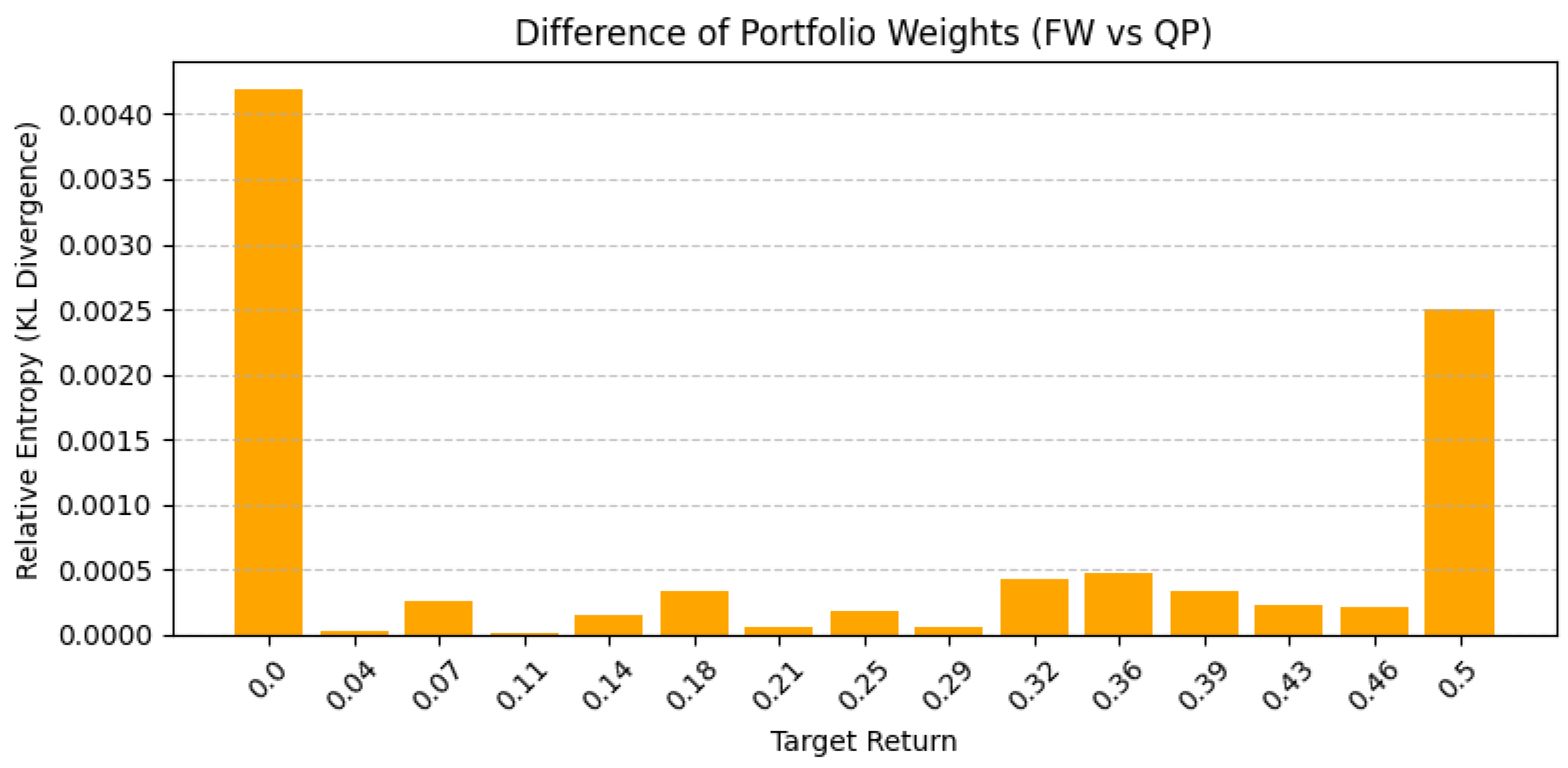
The numerical results presented in Table 5 summarize the portfolio variances and the relative entropy between the weight vectors obtained from both methods across a range of target returns. Relative entropy, also known as the Kullback–Leibler divergence, is used to measure the similarity between the two portfolio weight distributions, where a value of zero indicates identical distributions.
As shown in Table 5, the portfolio variances generated by the Frank-Wolfe algorithm are virtually identical to those produced by the CVXPY–OSQP solver across all target returns. Similarly, the relative entropy values are extremely small, generally very close to zero. This indicates that the weight distributions produced by the two methods are nearly indistinguishable, confirming that the Frank-Wolfe algorithm converges to the same optimal solution as the QP solver under the tested conditions.
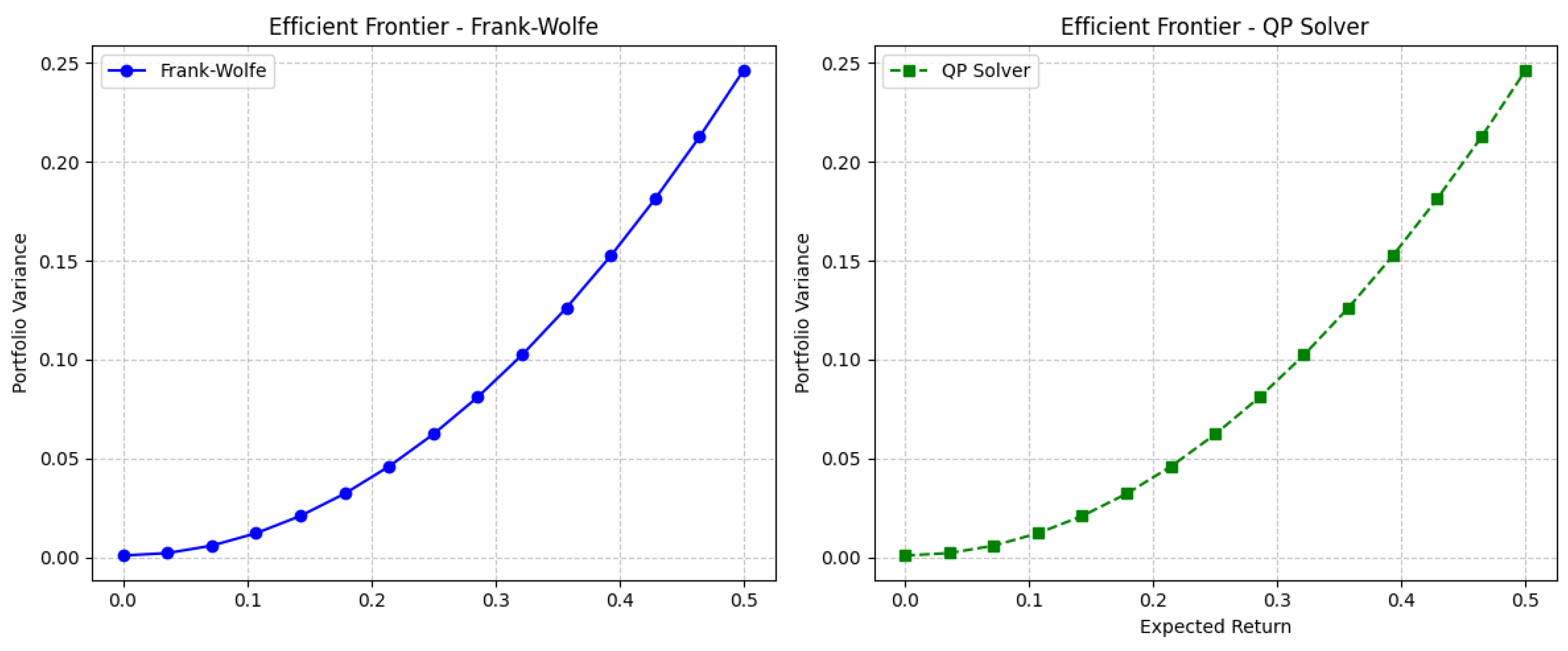
Figure 2 illustrates this similarity, where the efficient frontiers of both methods completely overlap. The absence of any visible divergence between the two curves visually confirms the equivalence of their solutions.
The use of relative entropy instead of Euclidean distance provides a more appropriate metric for comparing the portfolio weights, as it accounts for the probabilistic nature of the weights. Since the portfolio weights must sum to one and are non-negative, relative entropy captures even minor proportional differences in the distributions. In this case, the near-zero values indicate that both methods assign practically identical weights to each asset at every target return level.
As seen in Figure 3, the relative entropy remains consistently close to zero across the entire range of target returns, with the highest observed value being only 0.0042. This further supports the conclusion that the Frank-Wolfe algorithm effectively mirrors the optimal weight allocations found by the QP solver.
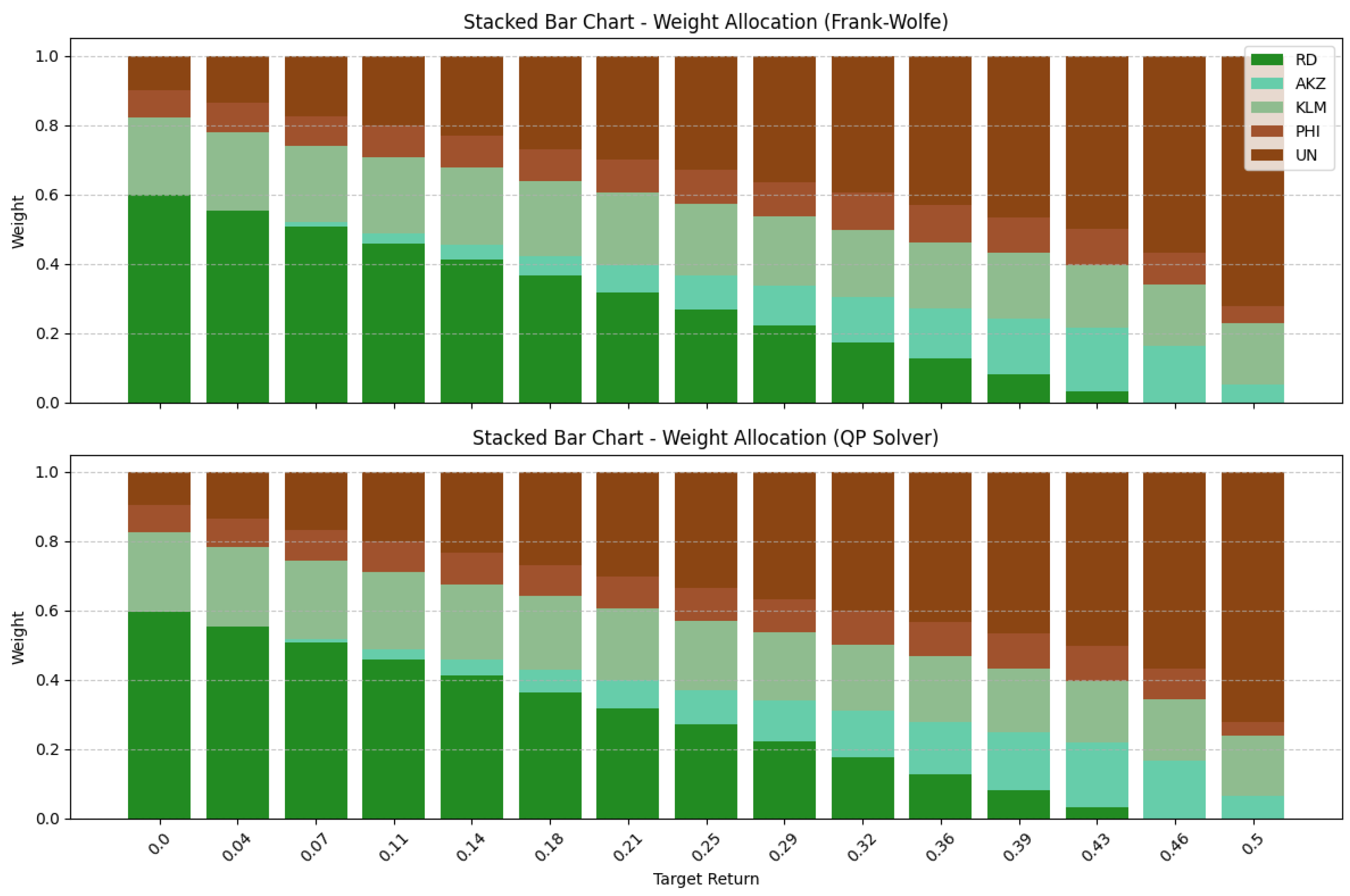
Furthermore, the individual portfolio weight trajectories, as shown in Figure 4, demonstrate virtually identical allocation patterns for each asset between the two methods. Assets such as Royal Dutch (RD) and Unilever (UN) follow the same shifting allocation patterns as target return increases, with other assets like AKZ, KLM, and PHI acting as diversifiers.
In summary, both the quantitative metrics and graphical visualizations confirm that the Frank-Wolfe algorithm, when properly implemented, can accurately replicate the solutions produced by the QP solver. The efficient frontier, portfolio variances, and weight allocations are indistinguishable between the two approaches. This demonstrates that Frank-Wolfe offers a computationally efficient alternative without sacrificing accuracy for small-scale problems.
These findings establish a solid foundation for extending the analysis to larger asset universes. While the five-asset case confirms accuracy, practical tactical allocation problems often involve hundreds or even thousands of assets. Therefore, in the following section, the scalability of both algorithms as n increases was examined, assessing how computational time, accuracy, and portfolio characteristics evolve as the problem dimension grows.

3.2.2. Portfolio Return and Risk Scaling

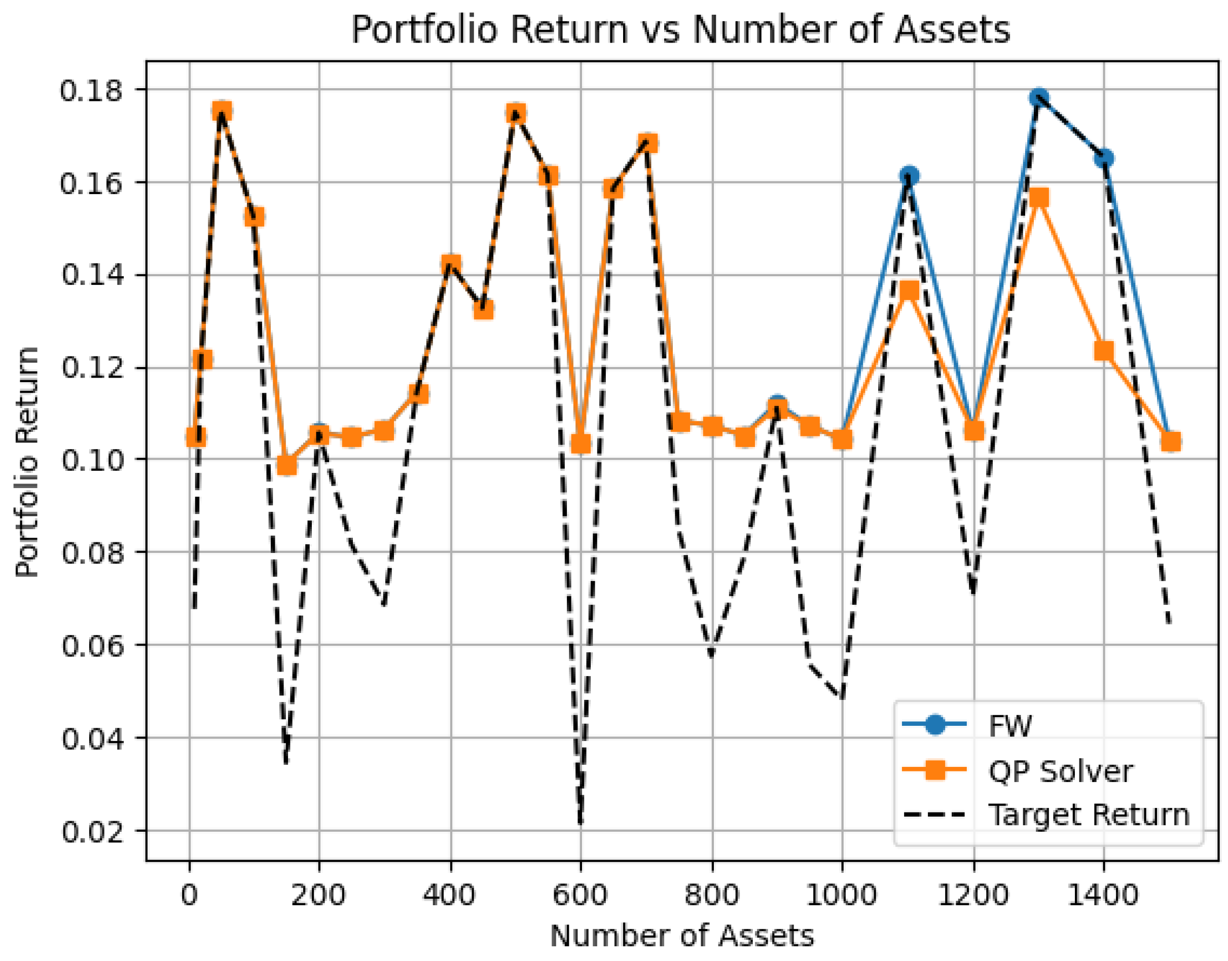
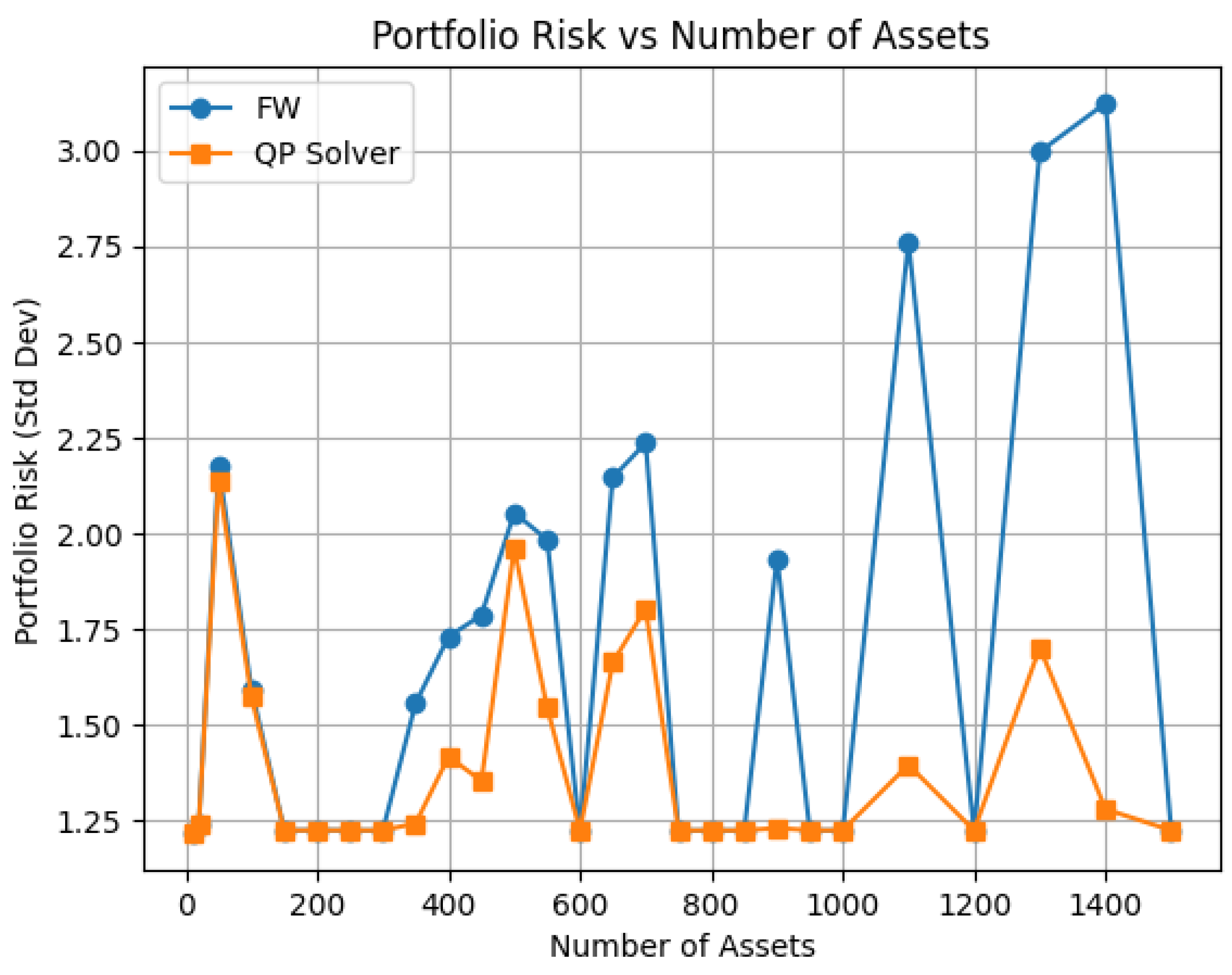
Figure 5 and Figure 6 along with Table 3 present how portfolio return and portfolio risk evolve as the number of assets increases for both FW and QP solvers. For small to moderate numbers of assets ( n 250 ), FW and QP produce virtually identical results, with overlapping curves for both return and risk. This confirms the consistency of FW with the exact QP solution in these settings.
As n grows beyond 300, slight deviations begin to emerge, especially in the highest return targets. At extremely large scales ( n > 900 ), the divergence becomes more pronounced for certain instances, indicating that while FW remains accurate for most cases, its iterative approximation can occasionally yield suboptimal solutions when the problem size is very high or when the target return is extreme. Despite this, the overall patterns of return and risk remain aligned, and the differences are negligible for typical portfolio allocation use cases.
Table 3 summarizes the return and risk comparison for selected problem sizes. Notably, the deviation observed for n = 1500 at the highest target return illustrates the first sign of instability, even though it remains within acceptable practical limits.
The nearly identical performance of FW and QP for small to medium asset universes reinforces the earlier findings from the five-asset case study, where the relative entropy between the weight distributions was effectively zero. This indicates that FW maintains accuracy while scaling to substantially larger problem sizes, making it a reliable approximation method for practical applications.

3.2.3. Execution Time Analysis

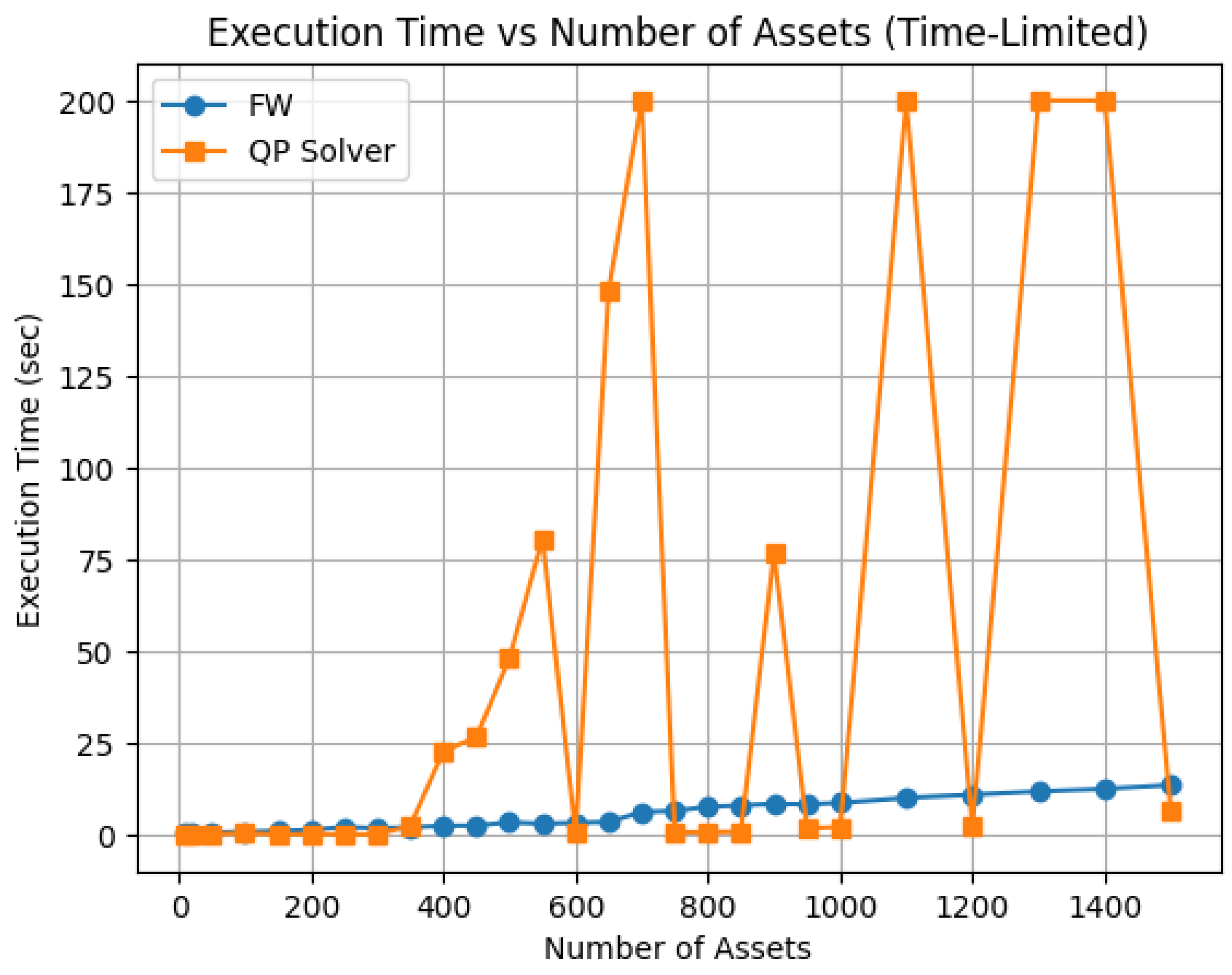
Figure 7 and Table 4 illustrate the computational time scaling behavior of both algorithms. For small problem sizes ( n 50 ), the QP solver is extremely fast due to the use of direct methods. However, as n grows, the computational burden of QP increases sharply, exhibiting near-exponential growth beyond n = 500 . Several large-scale instances reached the 200-second time limit, indicating severe scalability constraints.
In contrast, FW demonstrates a much slower growth rate in execution time. Even at n = 1500 , FW remained well within the time limit, with total runtime increasing smoothly as n grows. At n = 900 , FW is approximately 20 times faster than QP (4.32 s vs. 85.90 s), highlighting its scalability advantage. Table 4 shows execution times for the same subset of problem sizes.
The performance difference becomes stark at n > 900 , where FW maintains tractability while QP struggles. This indicates that FW’s iterative nature is better suited for very high-dimensional optimization compared to the direct matrix factorization methods used in QP.

3.2.4. Memory Usage Analysis

Figure 8 and Table 4 present the memory footprint comparison. FW shows a gradual, nearly linear increase in memory usage as the number of assets increases, as it primarily needs to store the gradient and a linear subproblem at each iteration. In contrast, QP requires storing dense Hessian matrices and other internal solver structures, causing memory to grow disproportionately.
For n > 500 , QP’s memory consumption escalates rapidly, exceeding 100,000 KB at n = 1500 . At this scale, QP uses nearly 8 times more memory than FW, making it unsuitable for constrained environments. FW remains consistently lightweight, reinforcing its suitability for cloud-based or embedded systems.
Note that peak memory numbers exhibit some run-to-run variability due to OS-level allocation behavior and solver internals, but the overall trend is clear. FW remains lightweight (tens of MB at largest n) while QP can require an order of magnitude more memory on many large instances.

3.2.5. Statistical Test for Execution Time and Memory Usage of FW and QP Solver

Table 6 summarizes the results of the runs test and Wilcoxon signed-rank test. The runs test assesses randomness in the sequences of execution time and memory usage, while the Wilcoxon test evaluates paired differences between FW and QP. To clarify the statistical hypotheses, the following null and alternative hypotheses were tested:
  • Runs Test
    H 0 : The sequence of observations is random.
    H 1 : The sequence of observations is not random (systematic trend).
  • Wilcoxon Signed-Rank Test
    H 0 : There is no difference in the paired distributions.
    H 1 : There is a systematic difference in the paired distributions.
The runs test rejects H 0 for FW’s runtime and memory usage ( p < 0.001 ), indicating that these metrics follow a clear increasing trend with problem size, while H 0 cannot be rejected for QP runtime ( p = 0.550 ), suggesting random-like fluctuations. For memory usage, both FW and QP exhibit systematic non-random growth.
Regarding efficiency, the Wilcoxon signed-rank test does not reject H 0 for execution time ( p = 0.348 ), implying no significant paired difference between FW and QP runtimes. However, for memory usage, H 0 is rejected ( p < 0.001 ), with a mean difference of 36,196 KB and a median difference of 21,340 KB. This confirms that FW consistently requires significantly less memory than QP, and that this result is due to systematic behavior rather than random variation.
The runs test indicates that FW’s runtime and memory usage grow with clear patterns as the problem size increases, while QP shows a random-like runtime progression but a strong memory trend. The Wilcoxon test confirms that FW requires significantly less memory than QP (mean difference = 36,196 KB, median difference = 21,340 KB, p < 0.001 ). The consistently negative differences indicate that FW’s memory footprint is systematically smaller across problem sizes, not due to random fluctuation.

3.2.6. Relative Gap Analysis

The relative optimality gap between FW and QP, shown in Figure 9, measures the deviation of FW’s solution from the exact QP optimum. Table 4 summarizes this for selected n values. For smaller problem sizes ( n 300 ), the gap is effectively zero, indicating an excellent approximation.
As n increases beyond 900, sporadic spikes appear in the gap, particularly at n = 1100 and n = 1500 . The maximum observed gap of 1.85% occurs at n = 1500 with the highest return target. In practice, this deviation remains acceptable, as typical industry tolerances for portfolio allocation are within the 2–5% range [2].
The combination of near-zero gaps for moderate sizes and rare, small spikes at extreme sizes demonstrates that FW maintains strong approximation quality across a wide range of portfolio configurations.
These results reveal a trade-off between computational efficiency and exactness. FW achieves substantial time and memory savings while maintaining excellent accuracy for most practical cases. For portfolios with up to 500 assets, FW matches QP almost perfectly. At very high dimensions, minor deviations may occur, especially under extreme return targets, but they remain within acceptable tolerances.

4. Conclusions

This study evaluated the performance of the Frank–Wolfe (FW) algorithm as an alternative to quadratic programming (QP) solved using the CVXPY–OSQP solver for tactical portfolio optimization. The evaluation focused on three key dimensions: solution similarity, computational runtime, and memory usage, across a range of portfolio sizes ( n = 50 to n = 1500 ) and varying target return levels.
The results demonstrate that FW closely replicates the QP solutions for small to moderate problem sizes. In the five-asset case study, portfolio variances and weight allocations from FW were virtually identical to those of the QP solver, confirmed by near-zero relative entropy values (Figure 3). This indicates that FW converges to the same optimal solutions under low-dimensional settings, making it an accurate substitute for exact quadratic solvers at these scales.
As the number of assets increases, FW continues to track QP closely up to approximately n = 500 . Beyond this point, slight deviations emerge, particularly at extreme target returns near the boundary of the feasible set. For very large portfolios ( n > 900 ), the differences become more visible. The maximum relative optimality gap observed was 1.85% at n = 1500 (Table 4). This suggests that while FW remains highly accurate for most practical cases, some degradation occurs under challenging high-dimensional scenarios with aggressive return targets.
From a computational perspective, FW exhibited substantial advantages. The execution time of FW scaled smoothly and predictably, remaining well below the imposed 200-s time limit even at the largest problem size tested ( n = 1500 ). In contrast, QP’s runtime increased sharply, exceeding the limit at n 1300 (Table 4, Figure 7). For example, at n = 900 , FW was roughly 20 times faster than QP (4.32 s vs. 85.90 s). This scaling behavior highlights FW’s suitability for large-scale applications where direct quadratic solvers become computationally infeasible.
Memory usage patterns reinforce this conclusion. FW’s memory footprint grew nearly linearly with n, reflecting its need to store only the gradient and a small set of linear subproblem structures. Conversely, QP’s memory demand rose disproportionately, driven by the storage of dense Hessian matrices and factorization structures. At n = 1500 , QP required over 150,000 KB, compared to just 17,713 KB for FW (Table 4). This eight-fold difference suggests that FW is particularly advantageous for deployment in resource-constrained environments, such as cloud computing platforms or embedded systems.
From a statistical perspective, formal non-parametric tests further reinforced these findings. The runs test indicated that FW’s execution time and memory usage follow non-random, structured growth patterns (Table 6), consistent with the smooth scalability trends observed in Figure 7 and Figure 8. By contrast, QP’s runtime exhibited random variation across scales, while its memory usage also showed non-random escalation, aligning with the solver’s increasing reliance on dense matrix factorizations.
The Wilcoxon signed-rank test revealed no statistically significant difference in execution times between FW and QP ( p = 0.348 ), despite FW’s smoother scaling behavior. However, the test confirmed a highly significant difference in memory consumption ( p < 0.001 ), with FW requiring systematically less memory across all problem sizes. The negative mean difference ( 36,196 KB) and median difference ( 21,340 KB) indicate that FW consistently consumed tens of megabytes less memory than QP. This statistical evidence substantiates the computational results, showing that FW’s lightweight memory requirements are not incidental but a robust property of the algorithm’s iterative structure.
Overall, the analysis quantifies a clear trade-off between precision and scalability. QP remains the gold standard for exactness, consistently delivering perfectly converged solutions across all scenarios. However, its computational and memory costs grow prohibitively at high dimensions. FW, on the other hand, offers dramatic gains in speed and memory efficiency while maintaining near-identical results for small to medium problem sizes and tolerable deviations for very large-scale cases. This balance makes FW an appealing alternative for tactical allocation tasks involving hundreds or thousands of assets, especially when fast, approximate solutions are sufficient.
Future research could explore adaptive or dynamic stopping criteria to improve solution quality without compromising efficiency. Additionally, extending the comparison to even larger portfolios and to robust optimization frameworks would provide deeper insights into FW’s performance under uncertainty. Given the observed advantages in speed and memory usage, FW holds strong potential for integration into real-time large-scale portfolio optimization systems.

Author Contributions

Conceptualization, D.P.S., D.C. and S.S.; methodology, D.P.S., D.C. and S.S.; software, D.P.S.; validation, D.P.S.; formal analysis, D.P.S.; investigation, D.P.S., D.C. and S.S.; resources, D.C. and S.S.; data curation, D.P.S., D.C. and S.S.; writing—original draft preparation, D.P.S., D.C. and S.S.; writing—review and editing, D.P.S., D.C. and S.S.; visualization, D.P.S.; supervision, D.C. and S.S.; project administration, D.C.; funding acquisition, D.C. All authors have read and agreed to the published version of the manuscript.

Funding

This research is supported by Universitas Padjadjaran Research Grant under Beasiswa Unggulan Pascasarjana Padjadjaran (Padjadjaran Excellence Fast Track Scholarship) entitled “Robust Optimization Model For Portfolio InvestmentWeight Using Frank-Wolfe Algorithm” with contract number 5086/UN6.3.1/PT.00/2024.

Data Availability Statement

The original data presented in the study are openly available in the following Google Colaboratory notebook at https://colab.research.google.com/drive/12DL9N0VL6cD3J10xn7zph-mdnDkviyNF?usp=sharing (accessed on 20 August 2025).

Acknowledgments

The authors are grateful to the Directorate of Research, Hilirization, and Community Engagement (DRHPM) of Universitas Padjadjaran for providing relevant support.

Conflicts of Interest

The authors declare no conflicts of interest.

References

  1. Sharpe, W.F. Capital asset prices: A theory of market equilibrium under conditions of risk. J. Financ. 1964, 19, 425–442. [Google Scholar] [CrossRef]
  2. Markowitz, H. Portfolio selection. J. Financ. 1952, 7, 77–91. [Google Scholar] [CrossRef]
  3. Bodie, Z.; Kane, A.; Marcus, A.J. Essentials of Investments, 12th ed.; McGraw-Hill Education: New York, NY, USA, 2018; Available online: https://www.mheducation.com/highered/product/Essentials-of-Investments-Bodie.html (accessed on 20 August 2025).
  4. Fabozzi, F.J.; Gupta, F.; Markowitz, H.M. The Theory and Practice of Investment Management, 2nd ed.; John Wiley & Sons: New York, NY, USA, 2010; Available online: https://www.wiley.com/en-us/The+Theory+and+Practice+of+Investment+Management%3A+Asset+Allocation%2C+Valuation%2C+Portfolio+Construction%2C+and+Strategies%2C+2nd+Edition-p-9780470929902 (accessed on 20 August 2025).
  5. Reilly, F.K. Investment Analysis and Portfolio Management; The Dryden Press: Orlando, FL, USA, 1989; Available online: https://www.researchgate.net/publication/31745765_Investment_Analysis_and_Portfolio_Management_FK_Reilly_KC_Brown (accessed on 20 August 2025).
  6. Elton, E.J.; Gruber, M.J.; Brown, S.J.; Goetzmann, W.N. Modern Portfolio Theory and Investment Analysis, 9th ed.; John Wiley & Sons: New York, NY, USA, 2014; Available online: https://www.wiley.com/en-us/Modern+Portfolio+Theory+and+Investment+Analysis%2C+9th+Edition-p-9781118469941 (accessed on 20 August 2025).
  7. Bisschop, J. AIMMS Optimization Modeling, Rev. ed.; John Wiley & Sons: New York, NY, 2021; Available online: https://documentation.aimms.com/_downloads/AIMMS_modeling.pdf (accessed on 20 August 2025).
  8. Blitz, D.; Hanauer, M.X.; Vidojevic, M. Global factor premiums. J. Portf. Manag. 2020, 46, 73–85. [Google Scholar] [CrossRef]
  9. Rompotis, G.G. Tactical asset allocation based on business cycle regimes. Int. J. Financ. Stud. 2020, 8, 45. [Google Scholar] [CrossRef]
  10. Markowitz, H.M. Portfolio Selection: Efficient Diversification of Investments; John Wiley & Sons: New York, NY, USA, 1959; Available online: https://www.wiley.com/en-us/Portfolio+Selection%3A+Efficient+Diversification+of+Investments%2C+2nd+Edition-p-9781557861085 (accessed on 20 August 2025).
  11. Boyd, S.; Vandenberghe, L. Convex Optimization; Cambridge University Press: Cambridge, UK, 2004; Available online: https://www.cambridge.org/highereducation/books/convex-optimization/17D2FAA54F641A2F62C7CCD01DFA97C4 (accessed on 20 August 2025).
  12. Lobo, M.S.; Vandenberghe, L.; Boyd, S.; Lebret, H. Applications of second-order cone programming. Linear Algebra Its Appl. 1998, 284, 193–228. [Google Scholar] [CrossRef]
  13. Bubeck, S. Convex optimization: Algorithms and complexity. Found. Trends Mach. Learn. 2015, 8, 231–357. [Google Scholar] [CrossRef]
  14. Boyd, S.; Parikh, N.; Chu, E.; Peleato, B.; Eckstein, J. Distributed optimization and statistical learning via the alternating direction method of multipliers. Found. Trends Mach. Learn. 2011, 3, 1–122. [Google Scholar] [CrossRef]
  15. Clark, E. Portfolio selection: A review. In Handbook of Key Global Financial Markets, Institutions, and Infrastructure; Elsevier: Amsterdam, The Netherlands, 2012; pp. 137–144. [Google Scholar] [CrossRef]
  16. Dom, M.S.; Howard, C.; Jansen, M.; Lohre, H. Beyond GMV: The relevance of covariance matrix estimation for risk-based portfolio construction. Quant. Financ. 2025, 25, 403–419. [Google Scholar] [CrossRef]
  17. Nesterov, Y. Lectures on Convex Optimization, 2nd ed.; Springer: Cham, Switzerland, 2018. [Google Scholar] [CrossRef]
  18. Lan, G.; Romeijn, E.; Zhou, Z. Conditional gradient methods for convex optimization with general affine and nonlinear constraints. SIAM J. Optim. 2021, 31, 2307–2339. [Google Scholar] [CrossRef]
  19. Frank, M.; Wolfe, P. An algorithm for quadratic programming. Nav. Res. Logist. Q. 1956, 3, 95–110. [Google Scholar] [CrossRef]
  20. Hillier, F.S.; Lieberman, G.J. Introduction to Operations Research, 7th ed.; McGraw Hill: New York, NY, USA, 2013; Available online: https://www.mheducation.com/highered/product/Introduction-to-Operations-Research-Hillier.html (accessed on 20 August 2025).
  21. Luenberger, D.G.; Ye, Y. Linear and Nonlinear Programming, 3rd ed.; Springer: New York, NY, USA, 2008; Available online: https://link.springer.com/book/10.1007/978-3-030-85450-8 (accessed on 20 August 2025).
  22. Ben-Ameur, H.; Saoud, M.; Zghal, S. Robust portfolio optimization with integer constraints and uncertain constraint coefficients. Eur. J. Oper. Res. 2020, 281, 177–191. [Google Scholar] [CrossRef]
  23. Buchheim, C.; De Santis, M.; Rinaldi, F.; Trieu, L. A Frank–Wolfe based branch-and-bound algorithm for mean-risk optimization. J. Glob. Optim. 2018, 70, 625–644. [Google Scholar] [CrossRef]
  24. Di Lorenzo, D.; Liuzzi, G.; Rinaldi, F.; Schoen, F.; Sciandrone, M. A concave optimization-based approach. Optim. Methods Softw. 2012, 27, 983–1000. [Google Scholar] [CrossRef]
  25. Wai, H.T.; Lafond, J.; Scaglione, A.; Moulines, E. Decentralized Frank-Wolfe algorithm for convex and nonconvex problems. Autom. Control 2017, 62, 5522–5537. [Google Scholar] [CrossRef]
  26. Thang, N.K.; Srivastava, S.; Tuan, H.D. Decentralized online Frank-Wolfe for portfolio management. IEEE Trans. Signal Process. 2022, 70, 1234–1247. [Google Scholar] [CrossRef]
  27. Dahik, C.A.; Al Masry, Z.; Chrétien, S.; Nicod, J.-M.; Rabehasaina, L. An SDP dual relaxation for the robust shortest-path problem with ellipsoidal uncertainty: Pierra’s decomposition method and a new primal Frank-Wolfe-type heuristics for duality gap evaluation. Mathematics 2022, 10, 4009. [Google Scholar] [CrossRef]
  28. Kumacheva, S.; Novgorodtcev, V. On the gradient method in one portfolio management problem. Mathematics 2024, 12, 3086. [Google Scholar] [CrossRef]
  29. Lopez-Dawn, R.; Giovanidis, A. Optimal influencer marketing campaign. IEEE Trans. Netw. Sci. Eng. 2023, 10, 1015–1031. [Google Scholar] [CrossRef]
  30. Chen, X.; Ge, D.; Wang, Z.; Ye, Y. Complexity of Frank-Wolfe methods for sparse portfolio selection. Oper. Res. 2020, 68, 682–695. [Google Scholar] [CrossRef]
  31. Lacoste-Julien, S.; Jaggi, M. On the global linear convergence of Frank-Wolfe optimization variants. In Advances in Neural Information Processing Systems; Curran Associates, Inc.: Red Hook, NY, USA, 2015; Volume 28, Available online: https://www.research-collection.ethz.ch/handle/20.500.11850/110467 (accessed on 20 August 2025).
  32. Firdaniza, F.; Ruchjana, B.N.; Chaerani, D.; Radianti, J. Information diffusion model in Twitter: A systematic literature review. Information 2021, 13, 13. [Google Scholar] [CrossRef]
  33. Moher, D.; Shamseer, L.; Clarke, M.; Ghersi, D.; Liberati, A.; Petticrew, M.; Shekelle, P.; Stewart, L.A.; PRISMA-P Group. Preferred reporting items for systematic review and meta-analysis protocols (PRISMA-P) 2015 statement. Syst. Rev. 2015, 4, 1. [Google Scholar] [CrossRef]
  34. Du, N.; Liu, Y.; Liu, Y. A new data-driven distributionally robust portfolio Optimization method based on Wasserstein ambiguity set. J. Optim. Theory Appl. 2021, 9, 3174–3194. [Google Scholar] [CrossRef]
  35. Jaimungal, S.; Pesenti, S.M.; Wang, Y.S.; Tatsat, H. Robust risk-aware reinforcement learning. SIAM J. Financ. Math. 2022, 13, 213–226. [Google Scholar] [CrossRef]
  36. Adhikari, R.; Putnam, K.J.; Panta, H. Robust Optimization-based commodity portfolio performance. Int. J. Financ. Stud. 2020, 8, 54. [Google Scholar] [CrossRef]
  37. Esteban-Pérez, A.; Morales, J.M. Distributionally robust stochastic programs with side information based on trimmings. Math. Program. 2022, 195, 1069–1105. [Google Scholar] [CrossRef]
  38. Statman, M. Finance for Normal People: How Investors and Markets Behave; Oxford University Press: Oxford, UK, 2017; Available online: https://global.oup.com/academic/product/finance-for-normal-people-9780190057121 (accessed on 20 August 2025).
  39. Hoang, T.M. Minimum variance portfolio in ASEAN-6 stock markets diversification: A Vietnamese perspective. Cogent Bus. Manag. 2022, 9, 2062909. [Google Scholar] [CrossRef]
  40. Aslanidis, N.; Christiansen, M.; Teresi, A. Correlation dynamics and portfolio diversification benefits. Int. Rev. Financ. Anal. 2016, 45, 177–186. [Google Scholar] [CrossRef]
  41. Fama, E.F.; French, K.R. A five-factor asset pricing model. J. Financ. Econ. 2015, 116, 1–22. [Google Scholar] [CrossRef]
  42. Chordia, T.; Goyal, A.; Sarno, L. Global market integration and the cross-section of expected returns. J. Financ. Econ. 2017, 123, 109–128. [Google Scholar] [CrossRef]
  43. Freund, R.M.; Grigas, P.; Mazumder, R. An extended Frank-Wolfe method with “in-face” directions, and its application to low-rank matrix completion. SIAM J. Optim. 2017, 27, 319–346. [Google Scholar] [CrossRef]
  44. Pokutta, S. The Frank-Wolfe algorithm: A short introduction. Jahresber. Der Dtsch. Math.-Ver. 2023, 126, 3–35. [Google Scholar] [CrossRef]
  45. Bomze, I.M.; Rinaldi, F.; Zeffiro, D. Frank–Wolfe and friends: A journey into projection-free first-order optimization methods. 4OR 2021, 19, 313–345. [Google Scholar] [CrossRef]
  46. Nocedal, J.; Wright, S.J. Numerical Optimization; Springer: New York, NY, USA, 2006; Available online: https://www.ime.unicamp.br/~pulino/MT404/TextosOnline/NocedalJ.pdf (accessed on 20 August 2025).
  47. Virtanen, P.; Gommers, R.; Oliphant, T.E.; Haberland, M.; Reddy, T.; Cournapeau, D.; van Mulbregt, P. SciPy 1.0: Fundamental algorithms for scientific computing in Python. Nat. Methods 2020, 17, 261–272. [Google Scholar] [CrossRef]
  48. Ben-Tal, A.; El Ghaoui, L.; Nemirovski, A. Robust Optimization; Princeton University Press: Princeton, NJ, USA, 2009; Available online: https://press.princeton.edu/books/hardcover/9780691143682/robust-optimization (accessed on 20 August 2025).
  49. Zhao, Z.; Ledoit, O.; Jiang, H. Risk Reduction and Efficiency Increase in Large Portfolios: Leverage and Shrinkage; Working Paper; University of Zurich, Department of Economics: Zürich, Switzerland, 2020. [Google Scholar] [CrossRef]
  50. Fabozzi, F.J.; Kolm, P.N.; Pachamanova, D.A.; Focardi, S.M. (Eds.) Robust Portfolio: Optimization and Management; John Wiley & Sons: Hoboken, NJ, USA, 2012. [Google Scholar] [CrossRef]
  51. Tütüncü, R.; Koenig, M. Robust asset allocation. Ann. Oper. Res. 2004, 132, 157–187. [Google Scholar] [CrossRef]
  52. Gorissen, B.L.; Yanıkoğlu, İ.; den Hertog, D. A practical guide to robust optimization. Omega 2015, 53, 124–137. [Google Scholar] [CrossRef]
  53. Mercurio, P.J.; Wu, Y.; Xie, H. Portfolio optimization for binary options based on relative entropy. Entropy 2020, 22, 752. [Google Scholar] [CrossRef]
  54. Hollander, M.; Wolfe, D.A.; Chicken, E. Nonparametric Statistical Methods, 3rd ed.; Wiley: Hoboken, NJ, USA, 2015. [Google Scholar] [CrossRef]
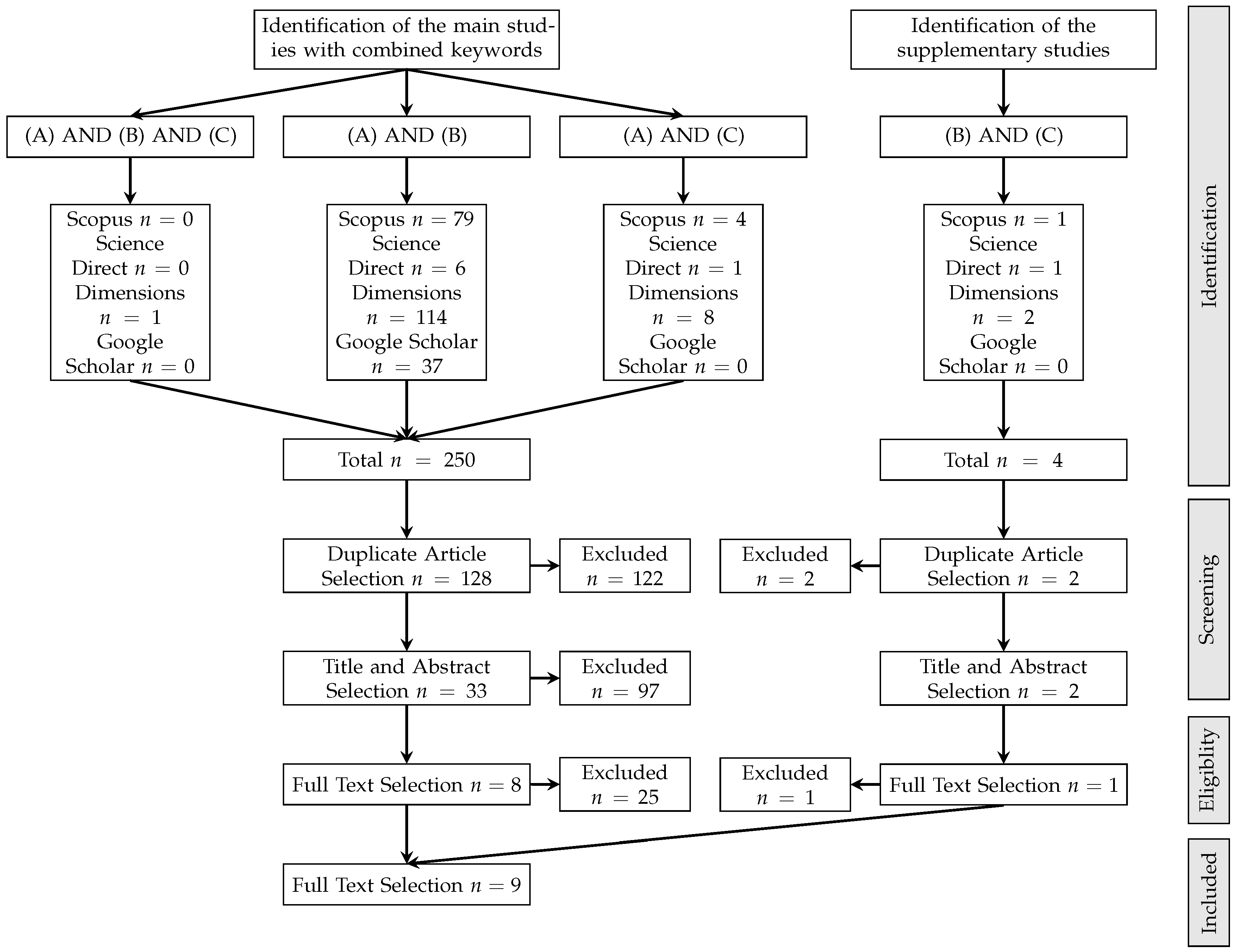
Figure 1. PRISMA Flowchart of the Systematic Literature Review Process.
Mathematics 13 03038 g001
Figure 2. Efficient Frontier Comparison: Frank-Wolfe vs. CVXPY–OSQP Solver.
Mathematics 13 03038 g002
Figure 3. Relative Entropy between Frank-Wolfe and QP Portfolio Weights.
Mathematics 13 03038 g003
Figure 4. Stacked Bar Chart of Portfolio Weight Allocation.
Mathematics 13 03038 g004
Figure 5. Portfolio Return vs. Number of Assets for FW and QP.
Mathematics 13 03038 g005
Figure 6. Portfolio Risk vs. Number of Assets for FW and QP.
Mathematics 13 03038 g006
Figure 7. Execution Time vs. Number of Assets (Time-Limited to 200 s).
Mathematics 13 03038 g007
Figure 8. Memory Usage vs. Number of Assets for FW and QP.
Mathematics 13 03038 g008
Figure 9. Relative Optimality Gap vs. Number of Assets.
Mathematics 13 03038 g009
Table 1. Summary of State-of-the-Art of the Selected Articles.
AuthorMethod/TechniquePUIPTIFWSM
[35]Uses a robust reinforcement learning approach with a Wasserstein-distance-based uncertainty set and policy gradient optimization.---Policy Gradient
[34]Reformulates bounded convex programming for robust optimization problems using a Wasserstein uncertainty set.---Bounded Convex Programming
[36]Utilizes Monte Carlo simulation-based robust optimization and mean-variance (MV) and conditional value-at-risk (CVaR) frameworks.--Simulation & LP
[37]Transforms partial mass transport problems using a pruning set and Wasserstein metric for distributional robust
optimization.
---Gradient Descent
[29]The Frank-Wolfe algorithm is applied to a convex optimization problem for influencer marketing with budget constraints.app.--LP
[27]Proposes a Frank-Wolfe-based heuristic for a robust discrete optimization problem under ellipsoidal uncertainty.--Heuristics & LP
[23]Frank-Wolfe-based algorithm and branch-and-bound method for mean-risk optimization.app.-Branch-and-Bound & LP
This
research
An Improved Frank–Wolfe Algorithm to Solve the Tactical Investment Portfolio Optimization Problemapp.First-Order & LP
Parameter Uncertainty (PU), Applicable (app.), Investment Portfolio Model (IP), Tactical Investment Portfolio (TI), Frank-Wolfe Algorithm (FW), Solving Method (SM). ✓: The feature/technique is present or used. -: The feature/technique is not present or used.
Table 2. Key Statistical Parameters of Five Dutch Stocks.
StockExpected Return ( m j )Standard Deviation ( σ j )
Royal Dutch (RD) 0.28 % 3.68 %
Akzo Nobel (AKZ) 0.33 % 3.45 %
KLM (KLM) 0.40 % 4.12 %
Philips (PHI) 0.30 % 4.21 %
Unilever (UN) 0.55 % 2.99 %
Table 3. Target Return, Portfolio Return, and Risk for FW and QP Solver.
nTargetFW ReturnQP Solver ReturnFW RiskQP Solver Risk
100.06760.10500.10501.21841.2184
200.12180.12180.12181.24311.2428
500.17520.17520.17522.17612.1379
1000.15240.15260.15231.59391.5733
1500.03440.09890.09891.22481.2248
2000.10560.10560.10551.22561.2250
2500.08150.10470.10471.22491.2250
3000.06850.10640.10641.22471.2247
3500.11440.11440.11431.55701.2432
4000.14220.14220.14211.73041.4172
4500.13250.13270.13241.78651.3542
5000.17480.17480.17482.05411.9599
5500.16150.16150.16141.98391.5460
6000.02130.10330.10331.22461.2246
6500.15840.15840.15832.14581.6631
7000.16850.16850.16822.23641.8040
7500.08470.10820.10821.22451.2245
8000.05740.10710.10721.22491.2249
8500.07860.10500.10511.22461.2246
9000.11100.11200.11101.93451.2307
9500.05550.10710.10711.22491.2249
10000.04790.10420.10421.22501.2250
11000.16120.16120.13672.76021.3959
12000.07040.10600.10601.22471.2247
13000.17820.17820.15652.99661.7024
14000.16510.16510.12343.12321.2801
15000.06440.10400.10401.22471.2247
Table 4. Execution Time, Memory Usage, and Relative Optimality Gap for FW and QP Solver.
nFW Time (s)QP Solver Time (s)FW Memory (KB)QP Solver Memory (KB)FW Relative
100.31900.003711,36020 2.73 × 10 7
200.37260.01582047 4.56 × 10 4
500.47080.067931216 3.61 × 10 2
1000.73510.374494800 2.64 × 10 2
1500.97210.01711961751 1.72 × 10 5
2001.22640.10733383076 9.19 × 10 4
2502.03970.03075174282 2.41 × 10 5
3001.70360.04707366133 1.93 × 10 5
3501.97302.35749959273 5.69 × 10 1
4002.373022.6763129212,081 4.91 × 10 1
4502.445926.5000162815,260 7.40 × 10 1
5003.338848.0849200418,810 9.84 × 10 2
5502.953280.5970241822,731 6.47 × 10 1
6003.21010.2577287124,211 3.46 × 10 6
6503.4351148.3290336431,688 6.65 × 10 1
7006.0909200.000 *389636,721 5.37 × 10 1
7506.43290.5636446637,731 3.30 × 10 6
8007.56500.6130507542,903 2.46 × 10 6
8507.92790.7248572448,406 2.92 × 10 6
9008.372976.8084641360,570 1.47 × 10 0
9508.25041.6698713960,408 7.15 × 10 7
10008.62432.0124790566,908 2.45 × 10 7
11009.9757200.000 *955590,367 2.78 × 10 0
120010.84562.207111,36096,247 4.46 × 10 7
130011.7348200.000 *13,322126,112 2.13 × 10 0
140012.4362200.000 *15,440146,211 4.83 × 10 0
150013.48646.611417,714150,216 1.85 × 10 7
* Reached imposed 200-second time limit.
Table 5. Comparison of Portfolio Variances and Relative Entropy of Weights.
Target ReturnVariance FWVariance QPRelative Entropy
0.00000.00080.00080.0042
0.03570.00210.00210.0000
0.07140.00580.00580.0003
0.10710.01210.01210.0000
0.14290.02090.02090.0001
0.17860.03210.03210.0003
0.21430.04590.04590.0001
0.25000.06220.06220.0002
0.28570.08100.08100.0001
0.32140.10230.10230.0004
0.35710.12610.12610.0005
0.39290.15240.15240.0003
0.42860.18120.18120.0002
0.46430.21250.21250.0002
0.50000.24640.24640.0025
Table 6. Summary of Statistical Test Results for FW and QP.
TestMetricMethodp-ValueInterpretation
Runs TestFW Time z = 4.904 <0.001Non-random trend
Runs TestFW Memory z = 4.493 <0.001Non-random trend
Runs TestQP Time z = 0.597 0.550 Random trend
Runs TestQP Memory z = 4.892 <0.001Non-random trend
WilcoxonExecution Time W = 149.0 0.348 No significant difference
WilcoxonMemory Usage W = 10.0 <0.001FW uses significantly less memory
Disclaimer/Publisher’s Note: The statements, opinions and data contained in all publications are solely those of the individual author(s) and contributor(s) and not of MDPI and/or the editor(s). MDPI and/or the editor(s) disclaim responsibility for any injury to people or property resulting from any ideas, methods, instructions or products referred to in the content.