Toward Optimal Multi-Agent Robot and Lift Schedules via Boolean Satisfiability

Abstract

As a multirobot system grows in its number of agents, contention over shared resources poses a more significant risk of deadlock and operational deficiencies. When integrating with buildings, one of the most common pieces of equipment that robots have to use is the lift (elevator). This work focuses on exploring different Anytime Constraint Programming techniques for finding time-optimal schedules across multiple robots and lifts. The choice of which lift each robot uses to complete its task has a noticeable impact on the makespan of the system. This work explores a Time-Ordered-based approach and a Time-Expansion Graph-based approach. The Time-Expansion Graph-based approach is found to outperform the Time-Ordered-based approach. This is because the Time-Expansion Graph method has immediate access to more comprehensive information. Additionally, this paper shows that, in some cases, applying such an optimization can considerably reduce the makespan.

1. Introduction

When deploying Multi-Agent Systems, robots may need to interact with resources around them, such as lifts, chargers, and work cells. The problem of planning robot task schedules that account for conflict-free utilization of such resources is NP-hard [1].

Previous work [2] proposed an approach to resource sharing between multiple robotic agents. The algorithm relied on encoding total ordering and optimizing a relaxed version of the problem. By trying different combinations, it was possible to gather more information. This allowed for the generation of a feasible schedule or a proof that a certain schedule was impossible.

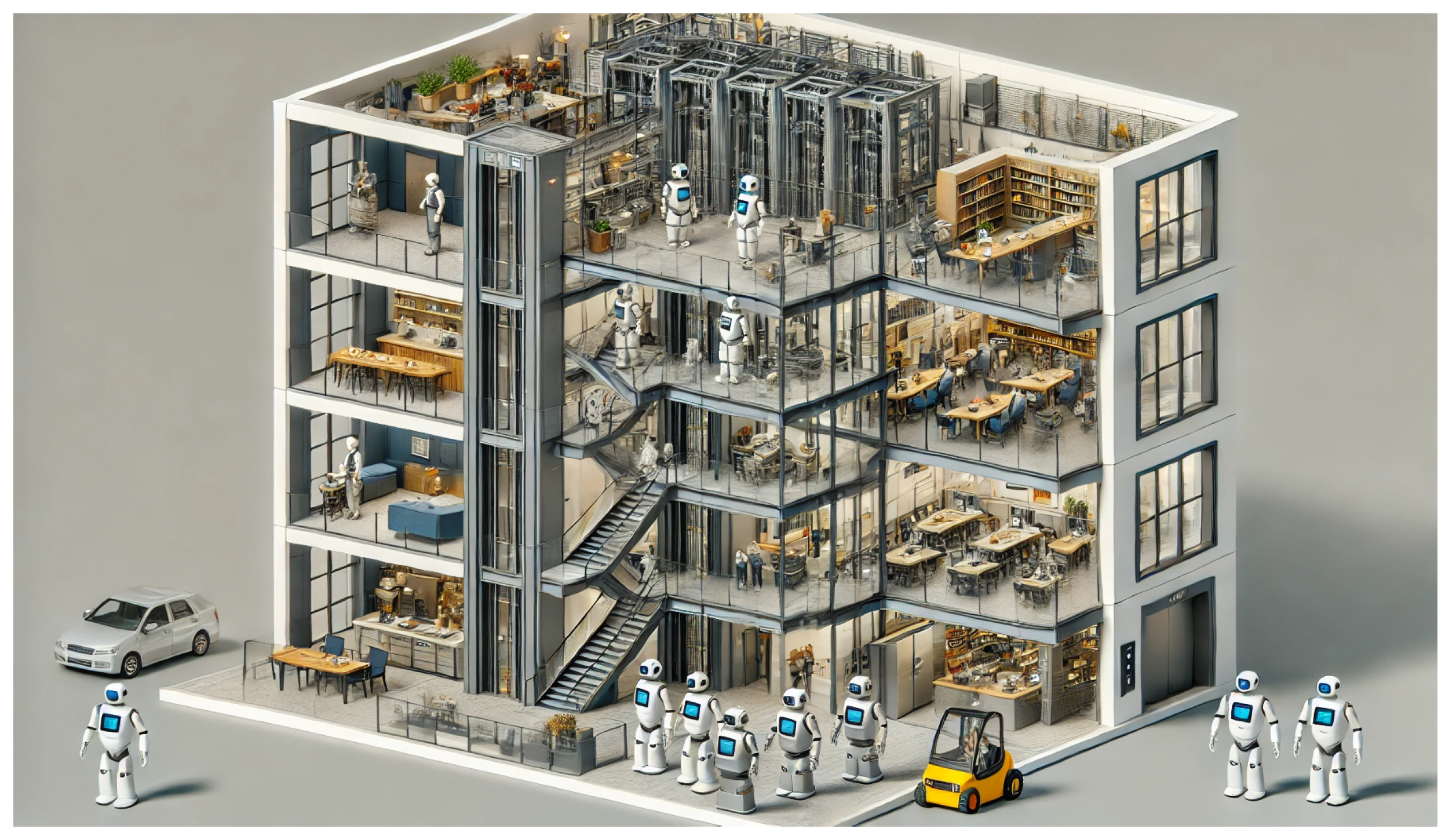
That work encoded the order as a strict total order into the SAT Conjunctive Normal Form (CNF) formulation and used that to solve the resource-ordering problem, relying on individual alternatives that have different costs independent of time. This paper applies similar ideas to the problem of scheduling the use of lifts (elevators) by autonomous agents. The aim is to create a lift schedule for robots and lifts that optimizes the total time spent. This problem frequently appears when robots are deployed in large facilities. For example, in a hospital, a robotic cart might be transporting dirty laundry from one area to another floor, while another robot delivers food to the wards. The building may have multiple lifts as shown in Figure 1. The use of lifts can become a crucial bottleneck for operations when the lifts are outnumbered by the robots that need to use them.

To address this kind of problem, it is necessary to extend the SAT-based encoding. This work builds on the formulation in [2], which is described in Section 4.2. It is also necessary to address the state-dependent nature of the resources. For example, if a lift drops a robot off at the 8th floor and then picks another robot up on the 9th floor, the process will be much faster than if it had to travel from the 9th to the 20th floor for the next pickup. This constraint is described in Section Adopting This Notation for the Lift-Optimization Problem.

This paper also shows a way to solve the resource-allocation problem using Time-Expansion Graphs (TEGs). The findings indicate that the TEG-based approach is better at finding optimality, while the Time-Ordered Encoding is better at finding feasibility. Finally, it is shown that optimal solutions reduce the makespan over other greedy strategies.

2. Related Work

Multirobot systems are increasingly deployed in the real world. The robotics community has developed a wide variety of tools to address these challenges. Much has been written on multi-agent path planning [3], task allocation [1], localization, and exploration [4]. As these systems are moved into the real world, ad hoc resource contention becomes an increasingly pressing issue [2]. Queuing systems have been proposed as a method of resolving such scenarios. Queuing systems are fundamental for successful robotic fleet management in unstructured environments [5]. However, spending too much time in queues is undesirable. The entire field of operations research is dedicated to studying how we can scale such operations [6]. Various methods exist to ensure that we obtain good enough quality solutions. For simple tasks without timing information or complex dependencies, it is possible to use the Khun–Munkres algorithm, which optimally solves these task assignments in $O\left(n^3\right)$ time [7]. However, in many cases, we are interested in a scenario where there are complex inter-dependencies of resources. This often turns such optimizations into NP-hard problems.

A variety of methods exist to solve such constraint-scheduling problems. While approaches like Mixed Integer Linear Programming (MILP) [8], often solved with commercial tools like Gurobi [9], are powerful for finding optimal solutions, and Reinforcement Learning (RL) [10] offers a way to learn scheduling policies, this work focuses on SAT-based approaches that can function as Anytime Algorithms [11]. An Anytime Algorithm can be stopped at any point to yield a valid, albeit potentially suboptimal, solution. This is a critical feature for real-world robotic systems, where a good-enough schedule delivered quickly is often preferable to a perfect schedule that takes too long to compute. Other methods like Ant Colony Optimization (ACO) and Genetic Algorithms (GA) can also produce good solutions, but they provide no optimality guarantees [12]. In contrast, the SAT-based methods explored here allow for a systematic search for optimality that can be truncated at any time. The focus of this work is to compare two different SAT-based anytime encodings, the Time-Expansion Graph and Time-Ordered methods, to understand their trade-offs. Constraint programming, using libraries like Google’s OR-Tools [13], was chosen for this work due to its ease of extension and its natural fit for modeling the logical constraints inherent in such multi-agent problems [14]. Within constraint programming, there are multiple ways of encoding resource-allocation problems. One commonly used method involves using Time-Expansion Graphs [3]. These have been used in compilation-based Multi-Agent Path Finding solvers [3]. An example of a Time-Expansion Graph that expresses lift usage can be seen in Figure 2a. To apply Time-Expansion Graphs to the lift-utilization problem, every lift will have to have a variable for every robot using a lift at every time step. Additionally, expressing task dependencies in the Time-Expansion Graph-based approach requires a large number of clauses, as rules must be enforced at every time step. In contrast, the Time-Ordered formulation can be expressed more efficiently because it does not need these time-discretized variables (see Figure 2b) [2].

3. Problem Statement

Given n robots that need to travel between floors and l lifts to transport them, the problem is to find a schedule that minimizes the makespan for all robot tasks. It is assumed that a lift can only service one robot at a time. This is a reasonable assumption as although multirobot lift rides could be possible, they are still challenging to achieve as coordinating the movement of robots entering and exiting the lift is a challenge. Even the single robot case is quite challenging from a motion planning and perception perspective [15].

3.1. Problem Analysis

This problem can be shown to be NP-hard by reducing it to the multiple Traveling-Salesman Problem (mTSP), where each robot is a city and each lift is a salesman. The mTSP is a known NP-hard problem [16].

3.2. Definitions

This work follows the same convention as established in [2]. The key idea here is that agents may request one of a given number of resources. Each resource may have an associated cost. For example, a robot may request access to a different floor via a lift.

• Each request can be defined as $R_i$.
• A request has n alternatives $R_i\left(j\right)=(s_{i,j},l_{i,j},r_{i,j},d_{i,j},c_{i,j}\left(t\right))$ where $s_{i,j},l_{i,j},d_{i,j}\in \mathbb{R}$. Each alternative is made of a start time s, a latest start time l, a  resource r, a cost $c\left(t\right)$ and a duration d.
• An alternative $R_i\left(j\right)$ cannot co-exist with alternative $R_k\left(m\right)$ if it shares the same resource (i.e., $r_{i,j}=r_{k,m}$) and the earliest end time of $R_i\left(j\right)$ is greater than the latest start time of $R_k\left(m\right)$

For makespan optimization, $c_{i,j}\left(t\right)$ is defined as $t_{i,j}$, where t is the time at which the reservation for the resource ends.

Adopting This Notation for the Lift-Optimization Problem

For the lift-optimization problem, it is assumed that there are n robots and m lifts. Every robot has a start point and a target point. There is an additional travel time from the start point to the lift and from the lift to the destination. This is encoded such that each robot makes one request $R_i$, with an alternative $R_i\left(j\right)$ for every lift. $R_i\left(j\right)$ is defined as $(s_{i,j},l_{i,j},r_{i,j},d_{i,j})$ where $j\in [1,\dots ,n]$ with the following parameters:

• $s_{i,j}$—The earliest start time is estimated by an A* search from the start point to the lift in question.
• $l_{i,j}$—The latest start time. Usually ∞, unless there is a deadline, in which case this would be the time given by the deadline minus A* from the lift in question to the target floor plus the duration it would take for the robot to use the lift.
• $r_{i,j}$—The lift in question.
• $d_{i,j}$—The duration for which the robot holds the lift. Often a function of the number of floors that the lift must traverse. For instance, if the robot needs to go from the 1st floor to the 10th floor and that takes 60 s, then this would be 60. Likewise, if the robot needs to go from the first to the second floor and that takes 20 s, this would be 20.

Notice that $c_{i,j}\left(t\right)$ is not defined, as this would just be the end time. This still does not fully capture the problem. It is necessary to find some way of defining the transition times between alternatives. For this, a transition matrix M is introduced. Each element $M_{(i,j),(k,m)}$ contains the cost of selecting alternative $R_i\left(j\right)$ after $R_k\left(m\right)$. If robot i requests lift j from the 7th floor to the 10th floor and robot k requests the same lift from the 11th floor to the 20th floor, then $M_{(i,j),(k,j)}$ would be the time to go between the 10th and 11th floors. This transition matrix can be precomputed in polynomial time. This matrix would then represent the constraint that there must be a minimum time gap of $M_{(i,j)(k,j)}$ between the start of $R_i\left(j\right)$ and $R_k\left(m\right)$.

Now that the time it will take for the robot to reach the destination floor has been encoded in the problem specification, the final destination must also be encoded. One way of doing this is that for every alternative, the lifts can request the robot’s time by treating the robot as a resource. The start time can be encoded into M for each of the reservations. In order to make things tractable, the lift will make a request $R_{k,m}$ for every alternative provided by the robot. $R_{k,m}$ will consist of two alternatives. The first is for the robot $R_{k,m}\left(0\right)$ in question that requests the lift, and the second is for a phantom resource $R_{k,m}\left(1\right)$. This phantom resource represents the fact that the robot does not have enough time to reach its destination or cannot be assigned. An additional constraint is added such that if and only if $R_k\left(m\right)$ is awarded, then $R_{k,m}\left(0\right)$ must be awarded.

4. Constraint Programming (CP) Algorithms for Solving the Robot Lift-Scheduling Problem

In this section, two constraint programming algorithms described to solve the robot lift-scheduling problem are described. The first is based on the notion of a Time-Expansion Graph and the second is based on the Time-Ordered Encoding.

4.1. Time-Expansion Graph Approach

As described earlier, Time-Expansion Graphs use discrete time steps to plan complex decision processes, defining a new decision variable for every time step. The Time-Expansion Graph approach to modeling this problem involved the following decision variables:

• A decision variable $x_{i,j,t}$ that means request i alternative j is being serviced at time t. (I.E at time t, $R_i\left(j\right)$ is being served)

Figure 3 demonstrates some of the constraints. Algorithm 1 provides a procedural overview of how the complete SAT formula is generated. The specific constraints are detailed below.

4.1.1. Resource Mutex Constraint

The simplest way of describing this is that at any point in time a resource may only service one request. This is shown in Figure 3 by (d) and can be formally described as: At any time t if $x_{i,j,t}$ and $x_{k,m,t}$ share the same resource, then $(\neg x_{i,j,t}\vee \neg x_{k,m,t})$ must hold.

4.1.2. Request Mutex

This is not described in Figure 3. However, it falls out of our original problem definition in Section Adopting This Notation for the Lift-Optimization Problem. Given a request $R_k$ only one alternative $R_k\left(j\right)$ can be satisfied. In CNF, this can be written as: “At any time t, for all $x_{k,j,t}$ and $x_{k,m,t}$ where $j=m$, $(\neg x_{k,j,t}\vee \neg x_{k,m,t})$ must hold”.

Algorithm 1 Time-Expansion Graph Constraint Generation

1: Input: Robots R, Lifts L, Time Horizon $T_{max}$ 2: Output: SAT Formula F 3: $F\leftarrow \mathrm{empty}\mathrm{formula}$ 4: procedure GenerateConstraints 5:     for all request $r\in R$ do  ▹Assignment Condition: Each request must be served 6:         $C\leftarrow \mathrm{empty}\mathrm{clause}$ 7:         for all alternative a of r do 8:             for all $t\in [0,T_{max}]$ do 9:                $C\leftarrow C\vee x_{r,a,t}$ 10:            end for 11:         end for 12:         $F\leftarrow F\wedge C$ 13:     end for 14:     for all lift $l\in L$ do      ▹ Resource Mutex: One robot per lift at any time 15:         for all $t\in [0,T_{max}]$ do 16:            for all pair of requests $(r_i,r_j)$ using l do 17:                $F\leftarrow F\wedge (\neg x_{r_i,l,t}\vee \neg x_{r_j,l,t})$ 18:            end for 19:         end for 20:     end for 21:     for all request $r\in R$ do         ▹Duration & Min-Gap Constraints 22:         for all alternative a of r with duration d do 23:            for all $t\in [1,T_{max}-d]$ do 24:                $is\_start\leftarrow (\neg x_{r,a,t-1}\wedge x_{r,a,t})$ 25:                $duration\_clause\leftarrow {\bigwedge }_{k=1}^d{x}_{r,a,t+k}$ 26:                $F\leftarrow F\wedge (is\_start\Rightarrow duration\_clause)$ 27:                for all other request $r^{\prime }\ne r$ using same lift as a do 28:                    $a^{\prime }\leftarrow$ alternative for $r^{\prime }$ using same lift 29:                    $gap\leftarrow M_{(r,a),(r^{\prime },a^{\prime })}$ 30:                    $mingap\_clause\leftarrow {\bigwedge }_{k=0}^{gap}\neg x_{r^{\prime },a^{\prime },t+d+k}$ 31:                    $F\leftarrow F\wedge (is\_start\Rightarrow mingap\_clause)$ 32:                end for 33:            end for 34:         end for 35:     end for 36: end procedure 37: return F

4.1.3. Assignment Condition

At least one alternative within a request must be satisfied. This can be written in CNF as (1).

$$\underset{m,t}{\bigvee }{x}_{k,m,t}$$

(1)

4.1.4. Duration Constraint

This constraint comes from the duration an alternative takes, i.e., $d_{k,j}$. As shown in Figure 3 (b), if we start at time (a), then we must mark the equivalent of $d_{k,j}$ time steps calculated based on the lift travel time between the start and destination floors. This can be expressed as the Boolean formula in (2).

$$(\neg x_{k,j,t-1}\wedge x_{k,j,t})\Rightarrow (x_{k,j,t+1}\wedge x_{k,j,t+2}\dots .\wedge x_{k,j,t+d_{k,j}})$$

(2)

4.1.5. Min-Gap Constraints

In Figure 3, this is shown by (c). Essentially, the travel time between the floor where the last robot was dropped off and where the next robot is picked up needs to be accounted for. This is expressed in $M_{(k,j)(m,n)}$. This results in a Boolean formula given in (3).

$$(\neg x_{k,j,t-1}\wedge x_{k,j,t})\Rightarrow (\neg x_{m,n,t+d_{k,j}}\wedge \neg x_{m,n,t+d_{k,j}+1}\dots .\wedge \neg x_{m,n,t+dur+M_{(k,j),(m,n)}})$$

(3)

A SAT instance is created with the above constraints up to a certain number of time steps. For example, a random walk could be used if no upper bound is set to estimate the time it would take to solve these instances. This would indicate if the solution is solvable in t seconds.

4.2. Time-Ordered Resource Allocation

The Time-Ordered approach in [2] suggests using total ordering constraints to estimate the order. Rather than immediately solving the whole problem, it tries to solve a relaxed version of the problem. The total ordering constraints are reproduced in the following section.

Let $x_{i,j}$ be the fact that $R_i\left(j\right)$ is assigned. The constraints (4) and (5) are added, which require that at least every reservation is granted.

$$(x_{i,0}\vee x_{i,1}\vee x_{i,2}\dots \vee x_{i,n})$$

(4)

$$\underset{j,k}{\bigwedge }(\neg x_{i,j}\vee \neg x_{i,k}),\mathrm{where}j<k$$

(5)

The ordering is also encoded using the strict ordering encoding described in the same paper. Let $X_{ijkm}$ be the fact that $x_{ij}$ is after $x_{km}$. Then, the anti-symmetry (6), transitivity (7) and connectedness (8) constraints are added:

$$\neg x_{ij}\vee \neg x_{km}\vee \neg X_{ijkm}\vee \neg X_{kmij}$$

(6)

$$\neg X_{ijkm}\vee \neg X_{kmnl}\vee X_{ijnl}$$

(7)

$$\neg x_{ij}\vee \neg x_{km}\vee X_{ijkm}\vee X_{kmij}$$

(8)

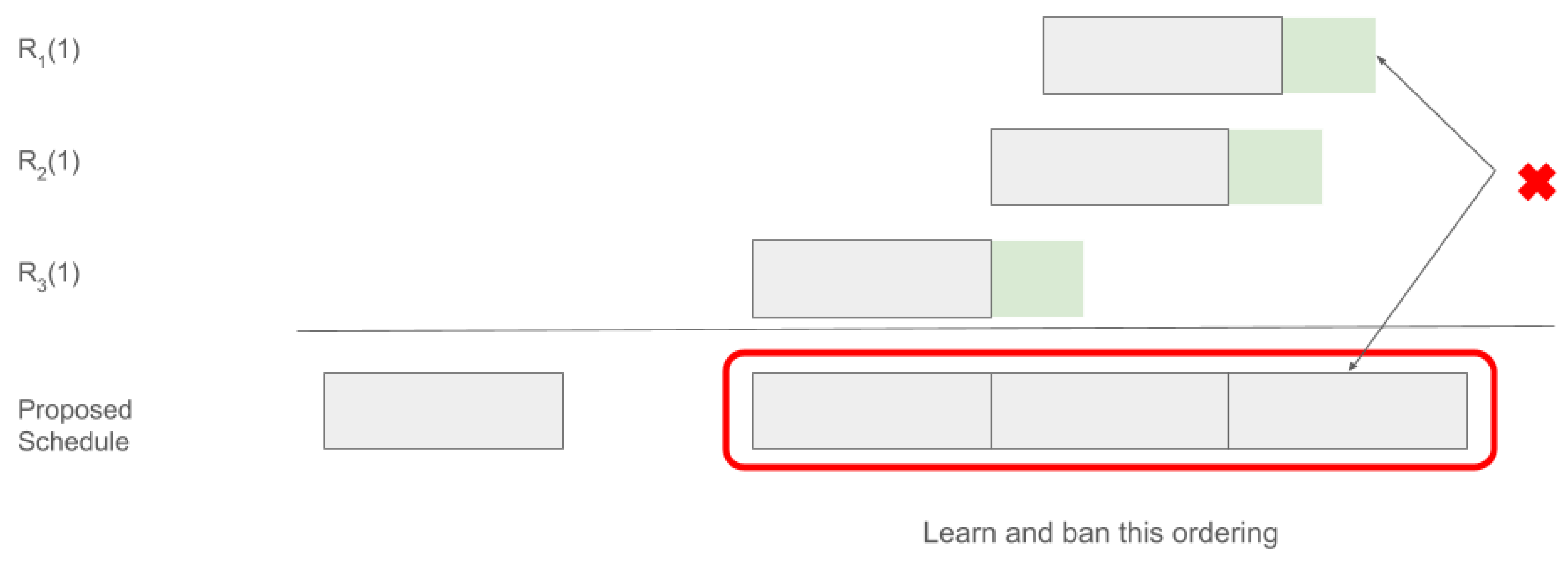
These constraints, when combined with the clause learning described in the previous paper, are sufficient for determining if a set of options is feasible. The method for clause learning is outlined in Algorithm 2. To  better understand how this works, suppose there is an order given by the constraint solver. To check if this order works, a schedule is constructed using a topological sort. In the event that the order does not work, a conflict arises, like the one shown in Figure 4. When this happens, it is learned that this given suborder does not work well. Backtracking can be done by simply looking at what caused the deadline for the last item to be exceeded. For instance, in Figure 4, $R_2\left(1\right)$ causes $R_1\left(1\right)$ to be pushed beyond its constraints. This can be seen as a reason to backtrack. It can be concluded that it is not possible to award both $R_2\left(1\right)$ and $R_1\left(1\right)$ in the same resource. This is essentially the group of reservations that cannot be awarded together. That constraint is added back into the solver and the process continues. The minimum time gap constraint is simply added to this backtracking process.

Algorithm 2 Conflict detection and clause learning for Resource Ordering

let $G(V,E)$ be the graph formed where V is the set of all the $x_{ij}$ assigned to be true and in resource $r\ast$, and  E is the set of all true $X_{ijkm}$. sorted_assignment ← topological_sort(G) schedule $\leftarrow \left\{\right\}$ banned_clauses $\leftarrow \left\{\right\}$ for all i in sorted_assignment.len() do     $s_i=$ sorted_assignment[i].earliest_start     $l_i=$ sorted_assignment[i].latest_start     if $s_i>$ schedule.last.end_time() then         schedule.insert_at($s_i$, sorted_assignment[i])     else if $l_i>$ schedule.last.end_time() then         $t\leftarrow$ schedule.last.end_time()         schedule.insert_at(t, sorted_assignment[i])     else         banned_clause ← ban_order()         banned_clauses.push(banned_clause)     end if end for return banned_clauses

4.3. Optimization with CP-SAT

Optimizing with CP-SAT can be done incrementally. One of the simplest ways to do this is by shrinking the time window [3]. This can be done for both the time-ordering method and the Time-Expansion Graph-based approach. Additionally, if only 2×-suboptimality is of interest, the windows can be shrunk more aggressively using a divide-by-two scale instead of incremental shrinking. The shrinking-time window-based approach guarantees an optimal makespan but may not guarantee an optimal sum of costs. Additionally, optimizing for the makespan of a single snapshot of problems does not guarantee that the makespan is optimized on a lifelong basis. With regard to this, the Time-Ordered formulation will inherently optimize the amount of time spent within every resource, as the algorithm will try to allocate the earliest free slot to the next item within a given resource while retaining a specific ordering. On the other hand, while the Time-Expansion Graph method guarantees the shortest makespan across all resources, individual resources may not necessarily have the shortest makespans. This is because a simple rectangular time window shrinking scheme is used. Within a resource, it may be further possible to optimize time by maintaining order and adhering to constraints in linear time.

5. Benchmarks

This section focuses on two primary benchmarks. The first assesses the impact of ignoring lift schedules on the performance of multirobot fleets: How does neglecting lift scheduling affect fleet behavior? The second evaluates scalability: Which approach, Time-Expansion Graph or Time-Ordered Encoding, scales better?

For the first benchmark, the optimal solutions are compared against a random walk approach. As expected, random walks are significantly slower than optimized solvers. However, the observed improvements are based on synthetic benchmarks, which are easier to control and generalize. Real-world benchmarks are more challenging, as results depend heavily on specific use cases, workloads, and environmental factors. This limitation highlights the importance of tailoring lift-scheduling optimizations to particular scenarios.

All benchmarks were performed on a 24-core AMD EPYC 7B12 processor with 96 GB of RAM running on Google Cloud in a single thread. The solver was written in Rust and used the Varisat SAT solver [17] under the hood. The source code for the solver is available on GitHub and integrated into the “rmf-reservation” library here: https://github.com/open-rmf/rmf_reservation (accessed on 3 September 2025).

5.1. Lift and Robot Models

Lift models tend to vary in speed. The fastest elevators in the world can travel at 9 ms⁻¹ [18], while a domestic elevator may travel at 0.15 ms⁻¹ [19]. In this benchmark, a model is used in which going from one floor to another has a constant speed of 15 s. Models for lifts in particularly tall buildings may need to account for acceleration when covering a large number of floors. It should be possible to model acceleration simply by tweaking the transition matrix M.

The robots are modeled as having a uniform distribution of travel times. While in reality robot arrival times are likely to have fixed modalities as pickups and drop-offs, since the optimization takes place over a short time, a uniform random distribution with travel times of up to 5 min is assumed. This is reasonable as the optimization is for a snapshot of a certain point in time. Robot arrival times in a building can vary depending on the distance traveled.

5.2. Solution Optimality

The first key question is “How necessary is optimizing lift allocation?” Using a simplified model, it was observed that optimizing lift schedules significantly improves performance compared to random allocation. For example:

• With 10 robots and 4 lifts, the improvement ranged from 4× to 8× faster.
• With 15 robots and 6 lifts, the upper bound increased to 6×.
• For 25 robots, performance gains exceeded 10×, with improvements continuing as robot density increased.

These results, while promising, are limited by the synthetic nature of the benchmarks. Real-world scenarios, influenced by specific tasks, robot capabilities, and environmental constraints, may yield different outcomes. This underscores the importance of further testing in operational settings to validate these findings.

5.3. Real-World Inspired Benchmark

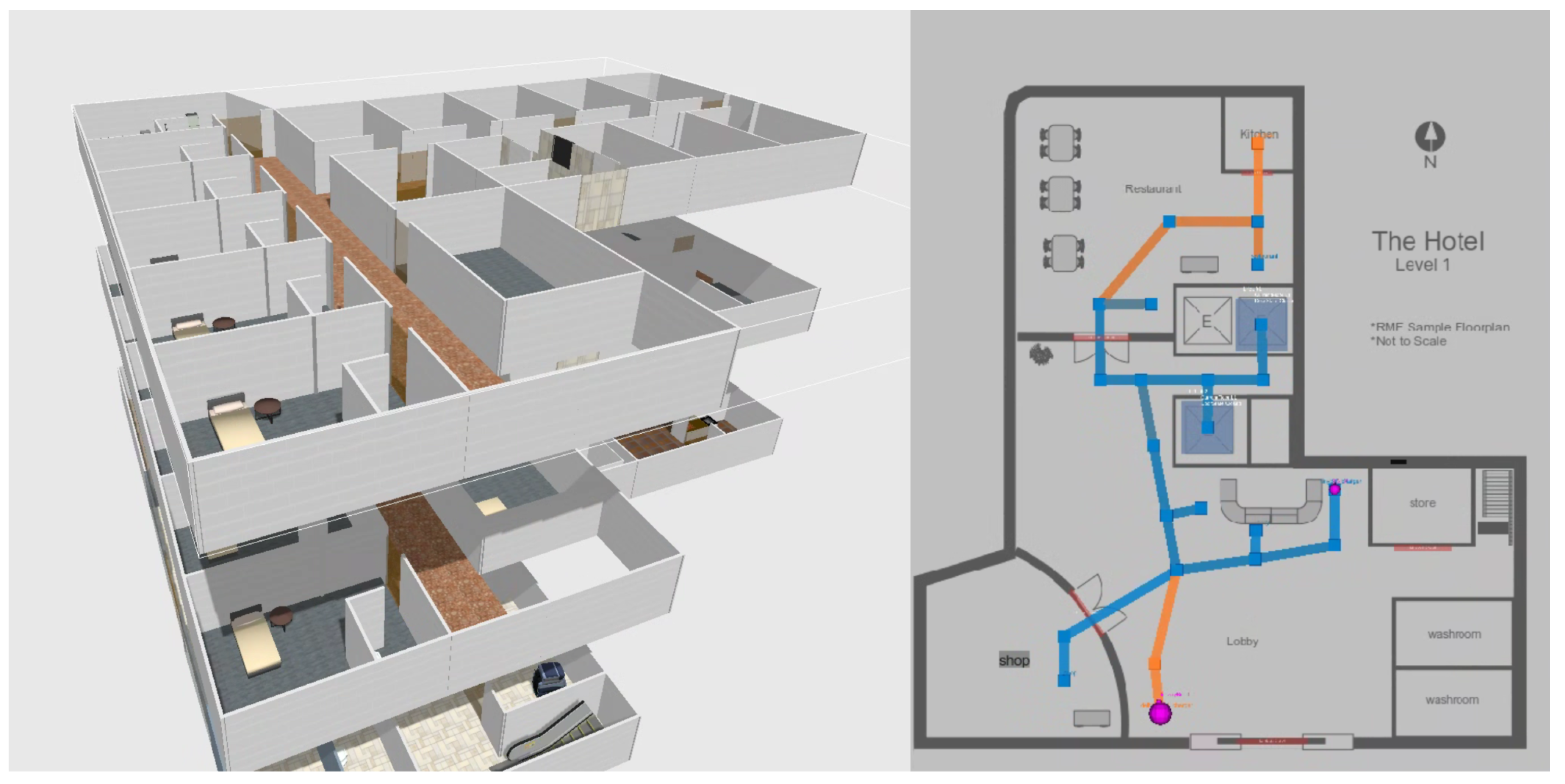
To study the effects of lift optimization, we use two demo worlds from Open-RMF [20]. The first, the hotel world (see Figure 5), features a single lift lobby with two lifts. This configuration mirrors a real-world scenario where lifts are located in close proximity, and thus the choice of a specific lift has a minimal effect on total travel time.

The second demo world is the hospital world (See Figure 6), which contains two distinct lift lobbies, each with 2 lifts. This environment is designed to highlight how selecting the appropriate lift lobby can lead to a substantial difference in task completion time. The higher number of lifts means that it is easy to simply allocate every robot to the unused lift, making the optimization easier.

The benchmarks involve spawning robots at various starting points determined by the navigation graph. Robots are randomly assigned a set of end points. This reflects a real world use-case where robots may be performing multi-drop off deliveries. For the purpose of optimality, we just relied on the Time-Ordered approach to compute optimal travel times.

5.4. Solution Optimality for Real World Benchmarks

The results of the real-world inspired benchmarks are presented in

Table 1. Hotel Scenarios: There are two lifts in a common lobby.

Scenario	Travel Time According to Greedy Algorithm (s)	Optimal Travel Time According to SAT (s)	Speed Up
Hotel-4-1	105	65	1.61×
Hotel-4-2	150	67	2.23×
Hotel-4-3	150	45	3.33×
Hotel-4-4	135	59	2.28×
Hotel-4-5	150	57	2.63×
Hotel-5-1	165	78	2.11×
Hotel-5-2	165	93	1.77×
Hotel-5-3	120	62	1.93×
Hotel-5-4	165	38	4.34×
Hotel-5-5	195	77	2.53×
Hotel-7-1	255	130	1.96×
Hotel-7-2	195	95	2.05×
Hotel-7-3	225	104	2.16×
Hotel-7-4	240	94	2.55×
Hotel-7-5	300	124	2.42×

and

Table 2. Hospital Scenarios: Four lifts are spread across two lobbies.

Scenario	Travel Time According to Greedy Algorithm (s)	Optimal Travel Time According to SAT (s)	Speed Up
Hospital-4-1	60	48	1.25×
Hospital-4-2	76	63	1.43×
Hospital-4-3	90	79	1.13×
Hospital-4-4	70	49	1.42×
Hospital-4-5	60	44	1.36×
Hospital-5-2	120	84	1.42×
Hospital-5-3	90	84	1.07×
Hospital-5-4	90	77	1.17×
Hospital-7-1	180	78	2.30×
Hospital-7-2	150	82	1.82×
Hospital-7-3	90	61	1.47×
Hospital-7-4	120	120	1.00×
Hospital-7-5	150	114	1.32×

. The scenarios are labeled `Environment-X-Y’, where `X’ denotes the number of robots and `Y’ is the trial number for that configuration. These tables compare the makespan of schedules generated by a greedy first-come-first-served algorithm against the optimal schedules found by the SAT-based approach.

In the Hotel scenario (Table 1), where two lifts share a common lobby, the SAT-based optimization yields significant improvements, with speedups ranging from 1.61× to 4.34×. On average, the optimal schedule is more than twice as fast as the greedy approach. This highlights the importance of intelligent sequencing, even when the choice of lift has minimal impact on travel time.

The Hospital scenario (Table 2) presents a different challenge, with four lifts spread across two lobbies. Here, the speedups are more modest, ranging from 1.00× (no improvement) to 2.30×. The availability of more lifts in separate lobbies means that the greedy algorithm can often make a locally optimal choice that is reasonably effective, reducing the performance gap. However, the SAT-based approach still consistently finds an equal or better solution, demonstrating its value in identifying globally optimal schedules that a greedy algorithm would miss, especially as the number of agents increases (e.g., scenario Hospital-7-1).

5.5. Time to Solve

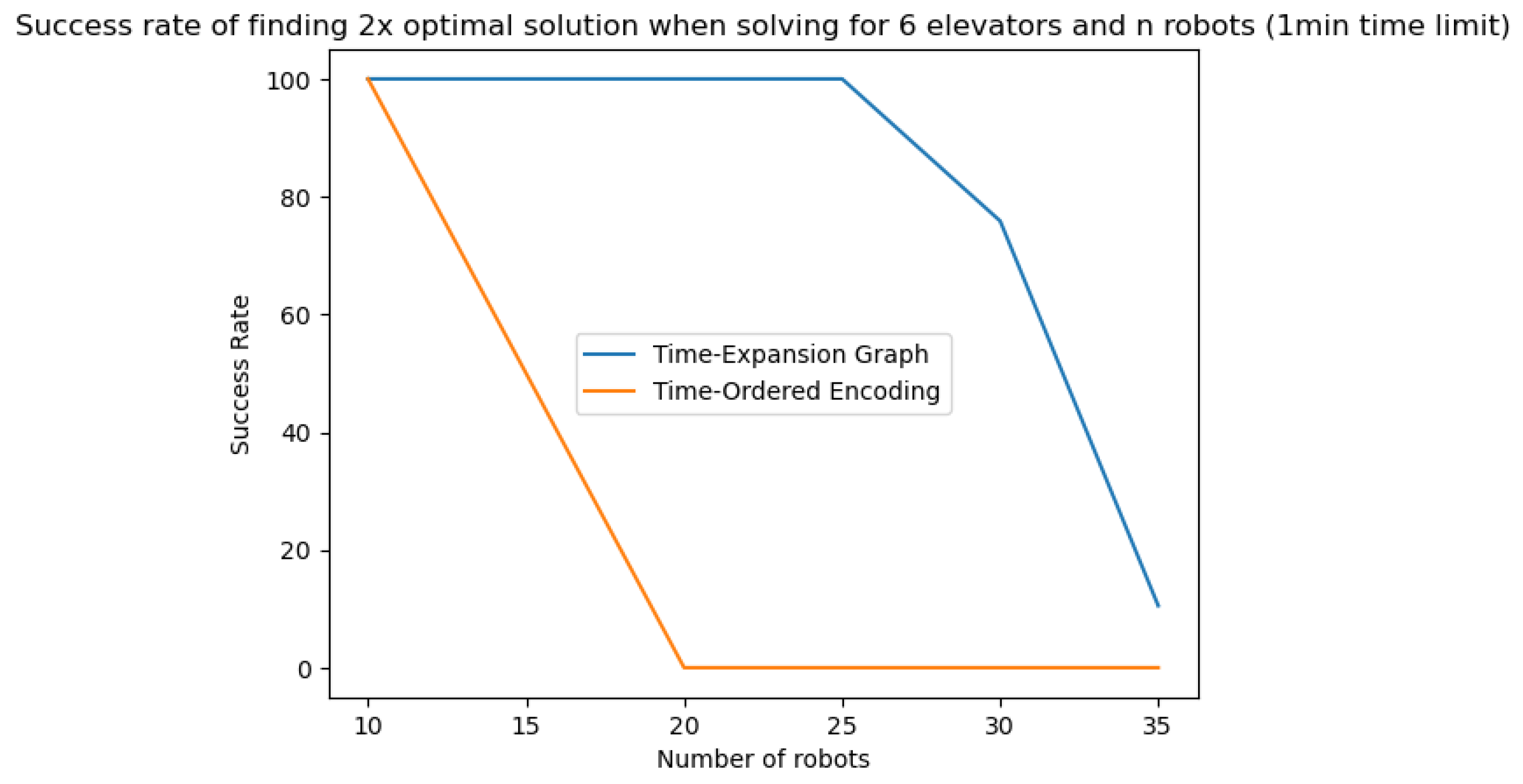
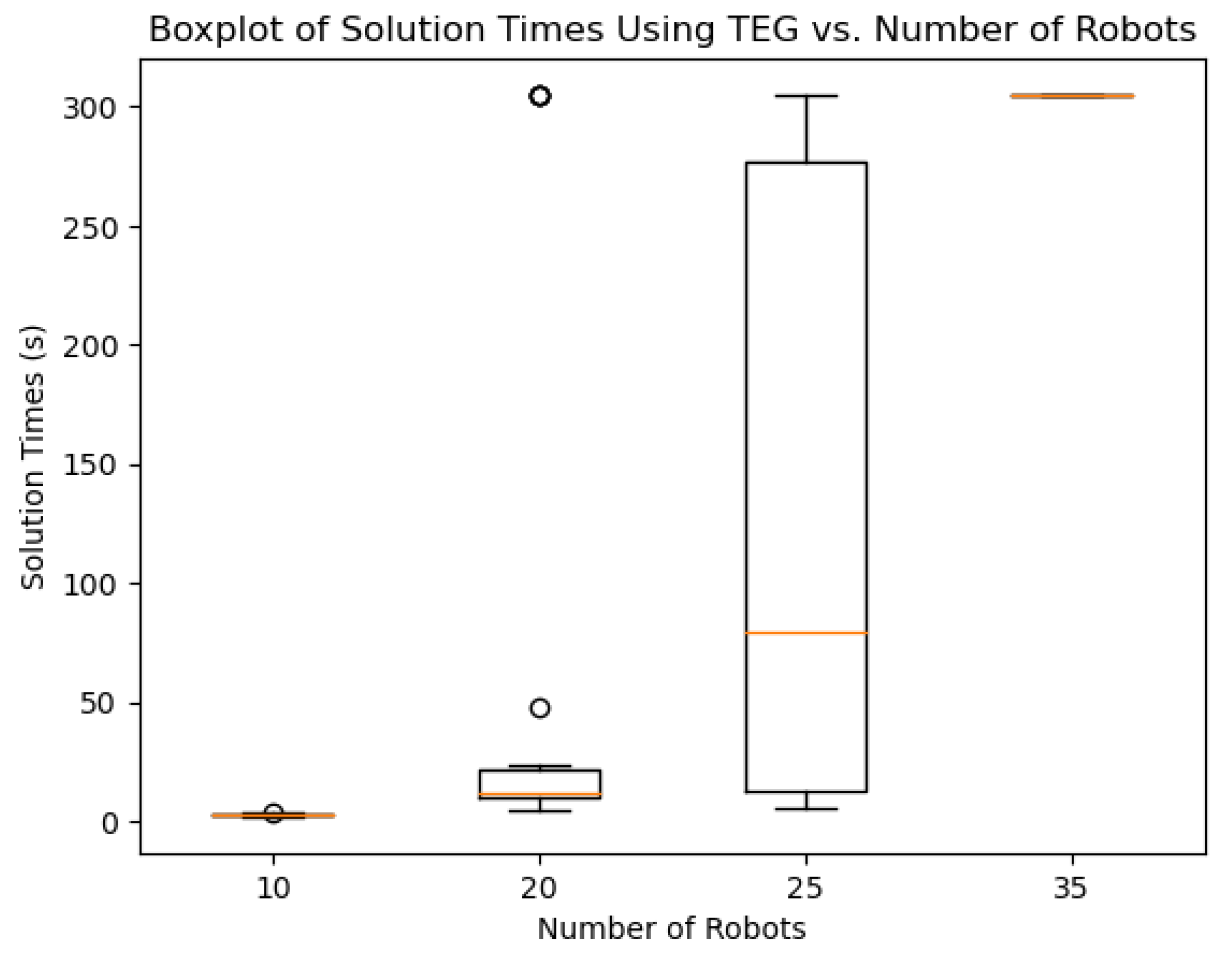
The time-optimal and 2×-suboptimal algorithms are compared using both Time-Expansion Graphs and Time-Ordered Resource Allocations. Initial benchmarks show that Time-Expansion Graphs can significantly outperform the Time-Ordered formulation for problems of medium size (see Figure 7). As the problems become larger, both Time-Expansion Graphs and Time-Ordered formulations struggle to cope with the scaling. As seen in Figure 7, when there are more than 25 simultaneous lift requests, it was found that the Time-Expansion Graph struggles with the encoding stage, as the encoding may take well over 30 s. 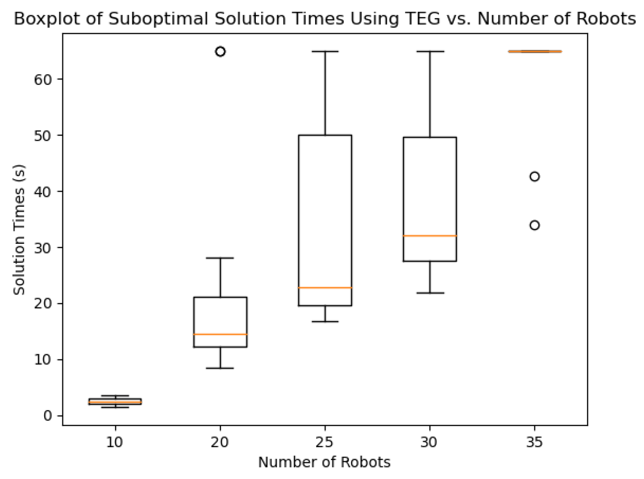The amount of time it takes to solve the problem may exceed the time savings proposed by the Time-Expansion Graph when 25 or more robots are involved (as shown in Figure 8). One way to mitigate this is to use 2× suboptimal solutions. This can lead to a significant speed up simply by tweaking the way the solver window is shrunk. If Figure 8 is compared to Figure 9, it is found that the amount of time taken to solve medium-sized instances is reduced by a factor of 5.

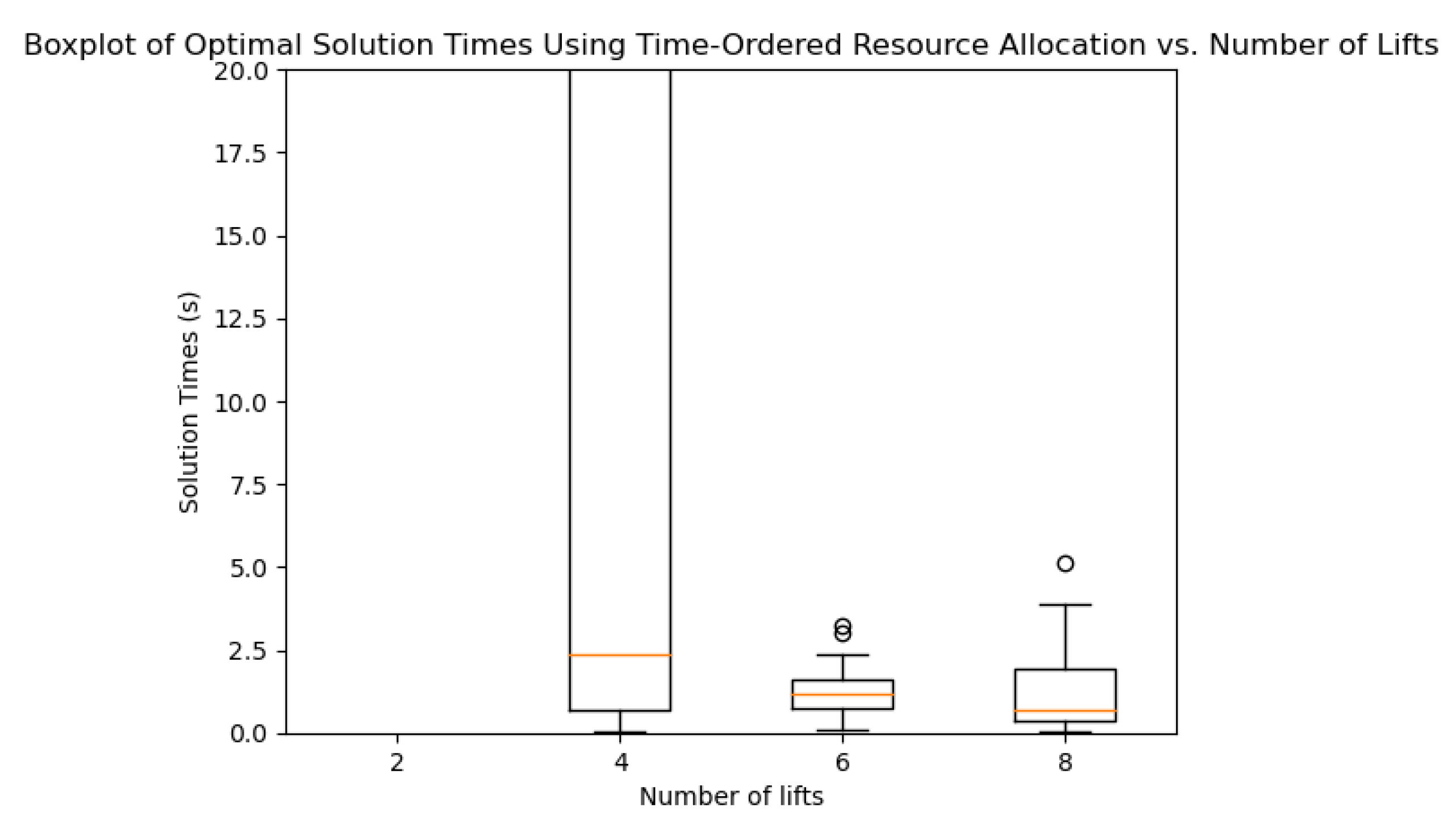
It is worth noting that the vast majority of runtime for the Time-Ordered Encoding was spent learning what did not work. Perhaps finding a way to “warm start” the solver with known impossible combinations may further improve performance. It may even be possible to exploit multi-core architectures to accelerate this, as discovering combinations of alternatives that do not work is an embarrassingly parallel problem. 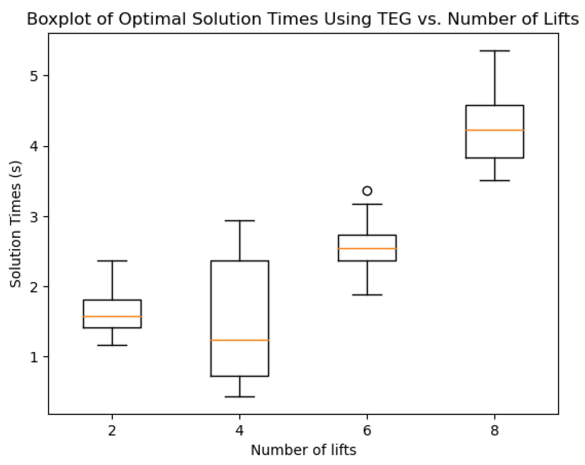Comparing Figure 10 and Figure 11, it is found that the behavior of Time-Expansion Graphs and the Time-Ordered Encoding are complementary to each other. As the number of lifts increases, Time-Expansion Graphs takes more time. This is expected, as the number of clauses increases greatly. As the number of lifts increases, the minimum time of $M_{(k,m)(n,l)}$ and encoding associated min-gap constraints takes up a significant amount of time. The opposite is found to be true for Time-Ordered Resource encoding. In fact, when there are more lifts, it is found that the performance of Time-Ordered Resource encoding improves.

6. Discussion

The results highlight a clear trade-off between the Time-Expansion Graph-based approach and the Time-Ordered approach. As shown in [2], the Time-Ordered approach is efficient in obtaining feasible solutions; however, the Time-Expansion Graph-based method is faster at obtaining optimal solutions. For the case of the lift-allocation problem, the latter is often more important than the former, as there is more interest in optimizing lift allocations. This suggests that Time-Expansion Graphs may be the better-suited method for the optimal lift-allocation problem. The superior performance of the Time-Expansion Graph approach can be attributed to its explicit representation of time, which is crucial in a tightly constrained problem like lift scheduling. The Time-Ordered method, while effective for feasibility, struggles to efficiently navigate the vast search space of possible orderings to find a time-optimal solution.

The real-world-inspired benchmarks further underscore this point. In both the Hotel and Hospital scenarios, the SAT-based solver consistently finds better schedules than the greedy approach. The results also indicate an upward trend in the performance gap as the number of simultaneous tasks increases. While these benchmarks are limited to seven tasks, this is primarily due to the prohibitive computation time required to find guaranteed optimal solutions for larger problems, as shown in our scalability analysis. This highlights a key trade-off: while the benefits of optimal scheduling become more pronounced with complexity, the computational cost also rises. For instance, if the number of robots simultaneously requesting lifts is less than the number of available lifts, a simple greedy heuristic or an assignment algorithm like Kuhn-Munkres may suffice. However, as the number of agents exceeds the number of resources, the method presented here becomes critical for avoiding significant bottlenecks.

The findings also have implications for real-world applications. In facilities like hospitals and hotels where lifts are a regular part of the workflow, it has been shown that lifts do form an important bottleneck. Thus, optimizing a robot’s usage of lifts will eventually become necessary. However, the solve times for larger problems indicate that there is a practical limit to the number of agents that can be scheduled in real-time using an optimal approach. For larger-scale deployments, the 2× sub-optimal solutions offer a practical compromise between performance and computational cost.

6.1. Handling Priorities and Dynamic Events

The proposed constraint programming framework can be extended to address dynamic, real-world operational challenges, such as task prioritization and resource malfunctions. The way this is done is independent of the underlying optimization method.

6.1.1. Handling Resource Outages

Since every request $R_i$ must be completed, a $R_{\mathrm{shutdown}}$ request can be created for the lift that is not in service with the appropriate parameters. The request should contain only one alternative. For every lift outage, a separate request $R_{\mathrm{shutdown}}$ would have to be created.

6.1.2. Handling Priorities

Priorities can also be handled in a similar way. Rather than processing all requests at once, the solver first handles the highest priority requests and then incrementally adds lower priority ones. It is important to note that the iterative shrinking window for optimization is only performed once the lowest-priority task is confirmed to be feasible.

7. Conclusions and Future Work

Two methods have been proposed to solve the optimal lift-scheduling problem. Additionally, it has been shown that 2× sub-optimal solutions can be found in a fraction of the time that is being optimized for via TEGs using a shrinking time window-based scheme. Suboptimal use of lifts can slow down the system, the exact amount depends on the frequency at which a robot uses a lift. While the methods described here work for small to medium deployments, there is still work to be done with regards to scaling. Several potential paths exist. First, the computation of potentially bad combinations in the Time-Ordered resource encoding can be parallelized. Second, the optimal solver can be used as a data generation tool to train a machine learning model. By generating a large dataset of complex scheduling problems and their optimal solutions, a learned heuristic could be developed to provide near-optimal schedules in real-time, bridging the gap between formal methods and the demands of dynamic, real-world environments. Finally, using a shrinking time window with incremental reduction may not be the best way to perform CP-Optimization. The potential use of binary search could be explored to reduce the number of times the Time-Expansion Graph-based method needs to call the SAT solver.

A key simplification in our model is the assumption that each lift carries only one robot at a time. Extending the framework to handle shared rides, while highly relevant for real-world efficiency, introduces significant scheduling complexity and is considered out of scope for this paper. In addition, in service settings such as hospitals, coordinating shared rides is challenging due to factors like intermittent network connectivity in lifts and unknown space constraints. This remains a complex problem that is a valuable direction for future investigation. Other constraints are also relevant, such as capacity constraints (e.g., a limited number of emergency parking spots on every floor) and spatial congestion, where each lift has a limit on how many robots can queue for it at one time.

Ultimately, the goal is to develop more generalized and user-friendly scheduling frameworks, paving the way for the seamless and efficient integration of autonomous systems into complex, human-centric environments.

References

- Gerkey, B.P.; Matarić, M.J. A formal analysis and taxonomy of task allocation in multi-robot systems. Int. J. Robot. Res. 2004, 23, 939–954. [Google Scholar] [CrossRef]
- Chakravarty, A.; Grey, M.; Muthugala, V.; Mohan, R. Time-Ordered Ad-hoc Resource Sharing For Independent Robotic Agents. In Proceedings of the 2024 IEEE/RSJ International Conference on Intelligent Robots and Systems (IROS), Abu Dhabhi, United Arab Emirates, 14–18 October 2024; pp. 879–888. [Google Scholar]
- Surynek, P.; Felner, A.; Stern, R.; Boyarski, E. Efficient SAT approach to multi-agent path finding under the sum of costs objective. In ECAI 2016; IOS Press: Amsterdam, The Netherlands, 2016; pp. 810–818. [Google Scholar]
- Dharmadhikari, M.; Nguyen, H.; Mascarich, F.; Khedekar, N.; Alexis, K. Autonomous Cave Exploration using Aerial Robots. In Proceedings of the 2021 International Conference on Unmanned Aircraft Systems (ICUAS), Athens, Greece, 15–18 June 2021; pp. 942–949. [Google Scholar] [CrossRef]
- Chakravarty, A. Open-RMF and the Challenge of Resource Contention in Large-Scale Robot Fleets. In Proceedings of the ROSCON, Odense, Denmark, 21–23 October 2024. [Google Scholar]
- Cook, W. In Pursuit of the Traveling Salesman: Mathematics at the Limits of Computation; Princeton University Press: Princeton, NJ, USA, 2014. [Google Scholar]
- Munkres, J. Algorithms for the assignment and transportation problems. J. Soc. Ind. Appl. Math. 1957, 5, 32–38. [Google Scholar] [CrossRef]
- Kondili, E.; Pantelides, C.C.; Sargent, R.W. A general algorithm for short-term scheduling of batch operations—I. MILP formulation. Comput. Chem. Eng. 1993, 17, 211–227. [Google Scholar] [CrossRef]
- Gurobi Optimization, LLC. Gurobi Optimizer Reference Manual; Gurobi Optimization, LLC.: Beaverton, Oregon, 2023. [Google Scholar]
- Dai, W.; Bidwai, A.; Sartoretti, G. Dynamic Coalition Formation and Routing for Multirobot Task Allocation via Reinforcement Learning. In Proceedings of the 2024 IEEE International Conference on Robotics and Automation (ICRA), Yokohama, Japan, 13–17 May 2024; pp. 16567–16573. [Google Scholar]
- Grass, J.; Zilberstein, S. Anytime algorithm development tools. SIGART Bull. 1996, 7, 20–27. [Google Scholar] [CrossRef]
- Shelkamy, M.; Elias, C.M.; Mahfouz, D.M.; Shehata, O.M. Comparative Analysis of Various Optimization Techniques for Solving Multi-Robot Task Allocation Problem. In Proceedings of the 2020 2nd Novel Intelligent and Leading Emerging Sciences Conference (NILES), Giza, Egypt, 24–26 October 2020; pp. 538–543. [Google Scholar] [CrossRef]
- Perron, L.; Furnon, V. OR-Tools (v9.12) [Software]. Google. 17 February 2025. Available online: https://developers.google.com/optimization/ (accessed on 3 September 2025).
- Vilím, P.; Laborie, P.; Shaw, P. Failure-directed search for constraint-based scheduling. In Proceedings of the Integration of AI and OR Techniques in Constraint Programming: 12th International Conference, CPAIOR 2015, Barcelona, Spain, 18–22 May 2015; Springer: Berlin/Heidelberg, Germany, 2015. Proceedings 12. pp. 437–453. [Google Scholar]
- Schulze, P.R.; Müller, S.; Müller, T.; Gross, H.M. On realizing autonomous transport services in multi story buildings with doors and elevators. Front. Robot. AI 2025, 12, 1546894. [Google Scholar] [CrossRef] [PubMed]
- Bektas, T. The multiple traveling salesman problem: An overview of formulations and solution procedures. Omega 2006, 34, 209–219. [Google Scholar] [CrossRef]
- Harder, J. Varisat. 2019. Available online: https://github.com/jix/varisat (accessed on 1 January 2025).
- The World’s 5 Fastest Elevators|Simplex|Simplex Elevators Australia|Lifting the Standard—simplexelevators.com.au. Available online: https://simplexelevators.com.au/2023/01/10/the-5-fastest-elevators-in-the-world/ (accessed on 11 December 2024).
- What Is the Speed of a Domestic Lift?—swiftlifts.com. Available online: https://swiftlifts.com/sg/swift-faq/what-is-the-speed-of-a-domestic-lift/ (accessed on 11 December 2024).
- OpenRMF Team. RMF Demos. Available online: https://github.com/open-rmf/rmf_demos (accessed on 3 September 2025).
Figure 1.
Fictional representation of the problem being solved: When multiple robots share the same set of lifts within a facility (generated by DALL-E).
Figure 2.
Comparison between Time-Expansion Graphs (a) and Time-Ordered Encoding (b), in Time-Expansion Graphs decision variable represent each agent at each time where as in the Time-Ordered Encoding, decision variable determine the order of resource usage.
Figure 3.
An example of what the decision variables mean and some of the constraints. (a) is the start of an awarded reservation, (b) shows the minimum number of time steps for the resource to be held (duration constraint) and (c) shows the duration for which other reservations must also be blocked because we awarded (a). This is calculated by the amount of time it takes for the floor where request 2 starts to be reached from the floor where request 1 drops the robot off (min-gap constraint). (d) demonstrates the resource mutex constraint—only one request can be serviced at a time.
Figure 4.
An example scenario in which backtracking is necessary. Here, three robots are trying to book the same resource. The green color indicates the latest end time for the reservations. In this case, having both and is not viable (as shown by the sequence of reservations in the red box overshooting the end of the green region in ).
Figure 5.
Hotel demo world taken from the Open-RMF demo maps. This world is used as an example of a real-world inspired benchmark. In the demo there are 3 floors: A lobby, and two hotel floors. This is an example of where choice of lift does not affect travel times; however, ift sequencing is still crucial for efficient pickup and drop-off [
20].
Figure 6.
Hospital demo world: Here, there are four lifts but the two lift lobbies are at two ends of the building [
Figure 7.
Success rate of Time-Expansion Graph vs. Time-Ordered Encoding: Here, the Time-Expansion Graph is found to scale to 25 simultaneous requests and 6 lifts without performance loss while the Time-Ordered scheme falls off very quickly.
Figure 8.
Time taken to find optimal solution using Time-Expansion Graph for 6 lifts. For each boxplot 50 samples were taken. The 35 robots size was unsolvable in the 5 min time-limit given. Box plot has the standard notation: The box represents the interquartile range, the horizontal line marks the median, the whiskers mark the minimum and maximum excluding outliers.
Figure 9.
2× Suboptimal solve times for the same scenarios as in
Figure 8. For each boxplot 50 samples were taken. The 35 robots size was unsolvable in the 5 min time-limit given. Box plot has the standard notation: The box represents the interquartile range, the horizontal line marks the median, the whiskers mark the minimum and maximum excluding outliers.
Figure 10.
Time-Expansion Graph solve times vs number of lifts in seconds. For each boxplot 50 samples were taken. Box plot has the standard notation: The box represents the inter-quartile range, the horizontal line marks the median, the whiskers mark the minimum and maximum excluding outliers.
Figure 11.
Time-Ordered Encoding optimal solve times vs number of lifts in seconds. For each box-plot 50 samples were taken. In each scenario there were 25 robots simultaneously requesting the same lift. Box plot has the standard notation: The box represents the inter-quartile range, the horizontal line marks the median, the whiskers mark the minimum and maximum excluding outliers. The case for 2 lifts exceeded the time limit for solving, while the upper end for 4 was at 80 s. The plot is scaled down, as it would be very hard to see the upper end of the spectrum for 6 lifts and 8 lifts otherwise.