Article

Vision-AQ: Explainable Multi-Modal Deep Learning for Air Pollution Classification in Smart Cities

1
Department of AI and Software, Gachon University, Seongnam-si 13120, Gyeonggi-do, Republic of Korea
2
Department of Creative Technologies, Air University, Islamabad 44000, Pakistan
*
Author to whom correspondence should be addressed.
Mathematics 2025, 13(18), 3017; https://doi.org/10.3390/math13183017
Submission received: 19 August 2025 / Revised: 10 September 2025 / Accepted: 16 September 2025 / Published: 18 September 2025
(This article belongs to the Special Issue Explainable and Trustworthy AI Models for Data Analytics)

Abstract

Accurate air quality prediction (AQP) is crucial for safeguarding public health and guiding smart city management. However, reliable assessment remains challenging due to complex emission patterns, meteorological variability, and chemical interactions, compounded by the limited coverage of ground-based monitoring networks. To address this gap, we propose Vision-AQ (Visual Integrated Operational Network for Air Quality), a novel multi-modal deep learning framework that classifies Air Quality Index (AQI) levels by integrating environmental imagery with pollutant data. Vision-AQ employs a dual-input neural architecture: (1) a pre-trained ResNet50 convolutional neural network (CNN) that extracts high-level features from city-scale environmental photographs in India and Nepal, capturing haze, smog, and visibility patterns, and (2) a multi-layer perceptron (MLP) that processes tabular sensor data, including PM 2.5 , PM 10 , and AQI values. The fused representations are passed to a classifier to predict six AQI categories. Trained on a comprehensive dataset, the model achieves strong predictive performance with high accuracy, precision, recall and F1-score of 99%, with 23.7 million parameters. To ensure interpretability, we use Grad-CAM visualization to highlights the model’s reliance on meaningful atmospheric features, confirming its explainability. The results demonstrate that Vision-AQ is a reliable, scalable, and cost-effective approach for localized AQI classification, offering the potential to augment conventional monitoring networks and enable more granular air quality management in urban South Asia.

1. Introduction

One of the most significant hazards to modern humans’ health worldwide is air pollution. By the World Health Organization (WHO), up to 7 million premature deaths occur each year as a result of the poor air that 99% of the world’s population breathes. Smart cities represent a novel approach to contemporary urban planning based on the use of human resources, cutting-edge technology, and cooperative sharing of data insights to improve the quality of life [1]. The idea of smart cities represents a source of optimism for an environmentally friendly environment as people in cities shift from one stage to the next. The principle of an smart city is a highly interconnected system where infrastructure, services, and innovations collaborate to raise people’s living standards [2]. Monitoring of air pollution is the foundation and fundamental requirement of environmental sustainability of smart city [3,4]. The quality of the air we breathe affects both our mental and physical health and therefore serves as essential for living [5]. Key air pollutants are fine particulate matter ( PM 2.5 ), ozone ( O 3 ), particulate matter ( PM 10 ), and nitrogen dioxide ( NO 2 ), which pose severe risks to the human respiratory and cardiovascular systems, also accelerating climate change and disturbing the ecological balance [6]. PM 2.5 is substantially smaller than PM 10 and other forms of airborne particles [7,8]. The human hair, with a diameter of 50–70 microns ( μ m), is significantly larger than both PM 2.5 and PM 10 particles [9]. Whereas PM 2.5 particles, consisting of compounds based on carbon and metallic substances caused by combustion, are smaller than 2.5 μ m in diameter, PM 2.5 particulates, which include pollen, dust, and molds, are less than 10 μ m [10].
Primary sources of air pollutants are CO, NO, SO 2 , NO 3 , PM 10 , and PM 2.5 globally. These pollutants are produced directly by industries, transportation, and animal husbandry, among other sources. While secondary pollutants, like O 3 , enter the atmosphere as a result of primary pollutants’ chemical interactions, air quality issues are aggravated. Active monitoring is required for legislation to regulate emissions, to protect human health, and to maintain the environment in a way that supports human well-being.
The development of technology to forecast region-wide air quality in the potential for smart city development opened up novel opportunities for visual-based (image-based) pollutants in the air control and surveillance, ranging from statistical models to modern Artificial Intelligence (AI) models [11]. CNN, AlexNet, LetNet, VGG-16, and ResNet-50 are frequently used to accurately forecast PM 2.5 and PM 10 levels using images in a smart city [12,13,14,15,16]. Real-time insight and preemptive steps to reduce air pollution are made possible by image-based categorization and air quality surveillance, which support the idea of an environment friendly smart city [17]. The significance of smart cities has grown in response to the environmental problems facing the world. Smart cities are able to track and enhance the quality of the air by using AI advancements in PM 2.5 predictions. The level of concentration of PM 2.5 levels in the metropolitan area of Kolkata is predicted by a researcher in the most recent study using a variety of ML models and statistical approaches, including XGBoost models, ridge regression, lasso regression, k-nearest neighbor (KNN), support vector regression (SVR), random forest (RF) regression, and decision trees. The XGBoost model continues to be the best-performing model, with improved linearity between observations and predictions. According to the study, the concentrations have shown significant seasonal variations in the PM 2.5 variables’ forecasting [18].
Zhou et al. [19] highlight the importance of accurately classifying air pollution and associated public health risks through the application of mathematical methods. We propose a novel, explainable multi-modal DL framework, the Vision-AQ, to bridge this data gap. Our approach moves beyond single-source analysis by synergistically fusing two distinct data modalities: (1) the qualitative, contextual features from ground-level environmental images and (2) the quantitative, precise measurements from corresponding pollutant label data. Vision-AQ is a dual-branch architecture, where a CNN interprets the visual information. At the same time, a parallel MLP processes the tabular label, and by combining these streams, the model learns a holistic representation of the atmospheric state to classify the local AQI accurately. In this study, we go beyond simply accuracy metrics and emphasis on model interpretability, and employ state-of-the-art explainable AI (XAI) techniques of Grad-CAM to dissect the model’s decision-making process, to verify that Vision-AQ is learning from logical environmental features, and to quantify the influence of each pollutant on its final prediction. Vision-AQ is explainable, multi-modal approach which is highly accurate and provides a transparent and trustworthy framework for augmenting sparse networks, paving the way for more granular and accessible air quality monitoring in the smart cities of the future. Air quality monitoring in rapidly urbanizing regions of South Asia, led by India, is critically hampered by a reliance on sparse and expensive networks of ground-based sensor stations [20].
Although the area has progressed due to the methods mentioned, there is still a significant lack of study at the border of explainability and multimodality [21]. Currently, AI-based studies use uni-modal data, depending solely on data from sensors, satellites, and ground visuals [22], and ignore the potential of integrating various distinct data sources. the combination of precise, quantitative info from a sensor with richer, contextual data from a visual outcome results in a more accurate and reliable prediction than either source alone [23]. The fusing of ground-level images with in-situ sensor readings is still an evolving and fascinating concerns with several recent research efforts have started investigating multi-modal fusion by integrating satellite and ground information [24]. Moreover, a requirement for explanation based on decisions with reliability is critical currently AI usage are more frequently in high-stakes environmental and public health applications [25,26]. Model outputs that lack justification are less likely to be trusted by scientists and policymakers. The field of XAI offers tools like Grad-CAM to peer inside the “black box,” but their application in environmental sensing is still not widespread.
Our research addresses the challenge of fusing two distinct yet complementary data modalities: the rich contextual information contained in ground-level environmental photographs and the precise quantitative measurements obtained from monitoring stations. The central problem is to design an intelligent system that can learn the complex non-linear relationships between visual cues such as haze and visibility and the corresponding pollutant concentrations. This must be achieved in a transparent and explainable manner to ensure that the resulting predictions are both trustworthy and interpretable. In this Study we address these gaps directly with Vision-AQ a multi-modal framework that explicitly fuses visual and label data. Crucially, by integrating XAI techniques throughout evaluation to ensure model is accurate, transparent, and interpretable, thereby building a foundation for more trustworthy AI in environmental science. With the objective of to design, develop, and evaluate Vision-AQ, an explainable multi-modal DL framework that classifies AQI by integrating ground-level environmental imagery with corresponding pollutant data to incorporates state-of-the-art explainable AI techniques to analyze the model’s decision-making process and verify that it generates distinct and separable clusters for different AQI categories. In addition, the study validates Vision-AQ as a practical approach to supplement sparse monitoring networks, providing a pathway toward more granular, accessible, and cost-effective air quality information in regions where data availability is limited.

2. Literature Review

2.1. Evolution of AQI

The progression of air quality monitoring (AQM) has followed a noteworthy trajectory, achieving key milestones motivated by the necessity to safeguard public health and the environment from the detrimental impacts of urban air pollution. Predicting air pollution has emerged as a critical component in the advancement of smart cities, presenting challenges that require immediate attention [27]. One of the core difficulties in accurate forecasting lies in the fluctuating nature of meteorological parameters, particularly wind speed and direction, which significantly influence pollutant dispersion. These factors are inherently dynamic, exhibiting continuous variation over time [28]. Over the years, the strategy for managing and observing air quality has evolved from addressing individual pollution events reactively to adopting a more proactive, integrated methodology supported by empirical research and technological innovations. Legislative responses to severe pollution episodes, such as the London Smog of 1952, led to pivotal policies like the UK’s Clean Air Act of 1956, which played a formative role in shaping early AQM practices [29]. Similarly, the United States began federal involvement in air quality regulation with the 1955 Air Pollution Control Act [30], eventually culminating in the Clean Air Act of 1970. This legislation laid the groundwork for a comprehensive framework to monitor, regulate, and enforce national ambient air quality standards [31].

2.2. Traditional and Sensor-Based AQM

The cornerstone of global AQM traditionally started from networks of fixed, ground-based monitoring stations covered in the study of [32]. Stations deployed by the Environmental Protection Agency (EPA) from governmental bodies to provide highly accurate, reference-grade measurements of criteria pollutants such as PM 2.5 , PM 10 , NO 2 , and O 3 . Data extracted from these stations are considered the gold standard and used for the calculation of the official AQI, as the basis for public health advisories and environmental policy [33]. The significant capital investment and operational costs associated with these stations lead to their sparse geographical distribution, creating vast areas in the developing nations and rural regions where there are no real-time air quality data [34]. Low-cost sensor (LCS) network devices have proliferated in recent years as a solution to this spatial gap, providing an affordable way to boost monitoring density, which includes individuals in the gathering of data [35]. However, promising for hyperlocal monitoring, sensor drift, cross-sensitivity to environmental factors like humidity, and the requirement for frequent co-location calibration against reference monitors to ensure data reliability are some of the significant issues that LCS networks frequently face [36].
Traditional AQM relies primarily on ground-based reference stations, which use high-precision instruments such as beta-attenuation monitors (BAM), tapered element oscillating microbalances (TEOM), and gas chromatography analyzers which provide accurate pollutant concentration measurements, but they are costly, energy-intensive, and geographically sparse [37]. which limit spatial coverage constrains their effectiveness in capturing localized pollution patterns, especially in developing regions. In response, LCS networks have emerged, providing scalable alternatives that allow denser deployments across cities in the PurpleAir, AirVisual, and Clarity sensor networks. While these sensors enhance coverage and enable community-driven monitoring, they suffer from calibration drift, environmental sensitivity, and limited long-term reliability [38]. but their growing adoption has enabled real-time urban monitoring and early-warning systems. These approaches laid the foundation for integrating IoT-based solutions into modern smart city infrastructures.

2.3. Satellite-Based Remote Sensing for Air Quality

Satellite remote sensing on a macro scale is a powerful tool for monitoring air pollution [34]. Satellite-based instruments such as MODIS (Moderate Resolution Imaging Spectroradiometer) and TROPOMI (Tropospheric Monitoring Instrument) measure Aerosol Optical Depth (AOD), which is statistically correlated with ground-level PM 2.5 concentrations [39]. In this approach, unparalleled global coverage becomes instrumental in understanding transboundary pollution and long-term exposure trends. However, this method has inherent limitations. Including that their spatial resolution is too coarse for intra-city analysis, and measurements were obstructed by cloud cover. Most importantly, their column-integrated measure of aerosols, and then converting to ground-level concentrations, required a complex modeling that introduces its uncertainties [40]. MODIS (Moderate Resolution Imaging Spectroradiometer), MISR (Multi-angle Imaging Spectroradiometer), and OMI (Ozone Monitoring Instrument) have been widely used to estimate aerosol optical depth (AOD), which serves as a proxy for surface-level particulate concentrations. These remote sensing methods enable long-term trend analysis, transboundary pollution tracking, and global exposure assessment [41]. satellite observations face challenges in temporal resolution, cloud interference, and limited vertical sensitivity. While daily global coverage is possible, the spatial resolution (1–10 km) often remains too coarse to inform localized interventions in urban neighborhoods. Recent work has improved estimation accuracy using ML models that fuse AOD with meteorological and ground-based measurements [42]. Still, the gap between satellite-derived data and fine-grained urban AQM persists, motivating alternative approaches.

2.4. Image-Based Air Pollution Estimation: Visual Sensing

A recent innovative approach, which involves leveraging the vast number of images captured daily from ground-level sources, including surveillance cameras, social media, and also personal devices, to visual cues in these images, such as atmospheric visibility, sky color, and image texture, is affected by the concentration of airborne particulate matter. Early research in this domain focused on deriving physical metrics from images. For example, research works by [43] used image processing techniques to estimate visibility distance correlated with PM 2.5 levels by using physical models. While effective, these methods are sensitive to image quality and lighting conditions for intelligent transportation systems. With the advent of artificial intelligence (AI), especially DL, research moved towards Convolutional Neural Networks (CNNs) to learn from the complex, non-linear relationship between extracted features from outside images and pollution levels directly [44]. Models like Air-CNN by [45], Deep-AIR by [46], and other custom architectures are trained on large datasets of outdoor images paired with sensor readings, using a hybrid CNN-LSTM. Structure to capture the spatio-temporal features. These studies have successfully demonstrated that CNNs can learn to see pollution and often outperform traditional image processing methods. Nonetheless, much of the available literature views the algorithm as a “black box,” emphasizing prediction accuracy without revealing the indicators that the model uses to form its conclusions [47,48,49].
With Visual sensing methods leverage consumer-grade devices such as CCTV, smartphones, and low-cost cameras to estimate air pollution levels which rely on detecting haze, light scattering, and color attenuation in images, which correlate with PM 2.5 and PM 10 concentrations. in a study DL models have been applied to extract atmospheric features from urban photos to predict pollutant levels with reasonable accuracy at low cost [50]. Compared to sensors and satellites, image-based methods provide ultra-localized information, as cameras can be easily deployed across dense areas. they also serve as complementary data streams for multimodal AI frameworks. still challenges remain, including lighting variations, occlusions, weather effects like rain, fog, which need for large annotated datasets. Despite these hurdles, visual sensing represents a promising low-cost, scalable alternative that bridges the gap between sparse monitoring stations and coarse satellite imagery.
Table 1 presents the classification of air quality based on selected pollutants, specifically AQI, PM 2.5 , and PM 10 , using the dataset employed in this study. The categories Good, Moderate, Unhealthy for Sensitive Groups, Unhealthy, Very Unhealthy, and Severe are adopted from the US EPA AQI guidelines of 2012 [51]. US EPA updated the upper limit of PM 2.5 for the “Good” category from 12 µg/m3 to 9 µg/m3 in 2023. However, since our dataset is labeled according to the earlier standard of both US EPA and Central Pollution Control Board (CPCB) [20,52], we also retained these definitions to ensure consistency with the source data. the AQI and pollutant concentrations in dataset is a as hourly measurements, which is directly associated with the corresponding image samples.
Our focus is on AQI, PM 2.5 , and PM 10 concentrations of air pollution parameters from the Table 1. While the dataset includes a broader range of pollutants such as O 3 , CO, SO 2 , and NO 2 , PM 2.5 and PM 10 are recognized as the most critical particulate matter indicators directly linked to respiratory and cardiovascular health risks. AQI serves as an aggregated measure that reflects overall air pollution levels and public health impact. By concentrating on these selected parameters, the analysis is streamlined to the most relevant factors affecting air quality and human health, enabling clearer insights and more targeted pollution mitigation strategies.

3. Methodology

This study proposes and evaluates Vision-AQ, an explainable multi-modal DL framework for air quality classification. Methodology is structured into four key phases: (1) data acquisition and pre-processing, (2) the Vision-AQ model architecture, (3) a two-stage training and fine-tuning strategy, and (4) a framework for performance evaluation and model interpretability.
For a visual understanding of the dataset, we print the sample images from each class are shown in Figure 1 which illustrate visibility and sky color varying in all six classes. to validate the class distribution in the dataset, we also examined representative images from each AQI category, as presented in Figure 1. These samples demonstrate the visual differences across Good, Moderate, Unhealthy, and Severe conditions, which form the basis for the classification task. where each row corresponds to a different AQI class. These samples highlight the progressive visual degradation of air quality as pollution levels increase.

3.1. Exploratory Data Analysis

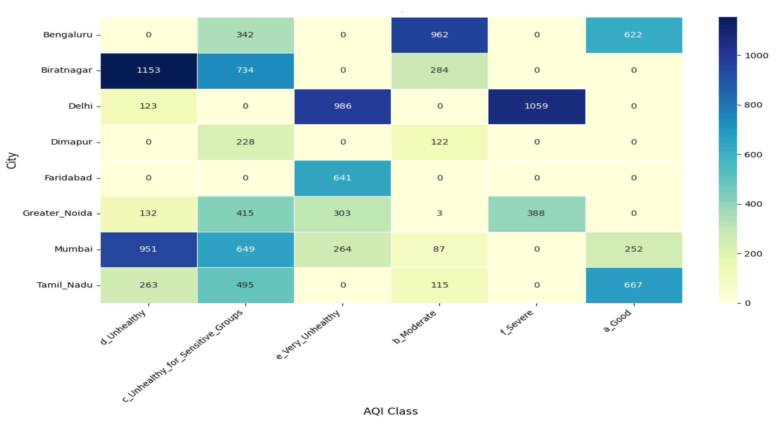
Figure 1 shows the Exploratory Data Analysis (EDA) of the Vision-AQ Dataset. In contrast, Figure 2 shows the distribution of images across each city and AQI class, revealing a significant concentration of data in specific categories for cities like Delhi and Bengaluru.
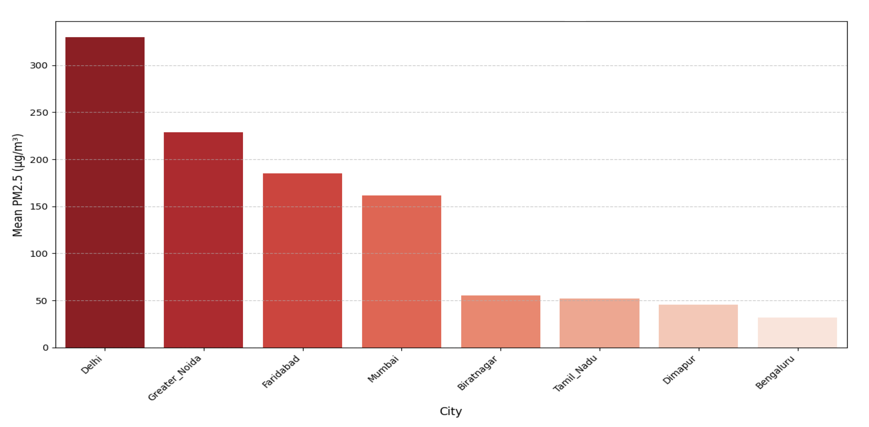
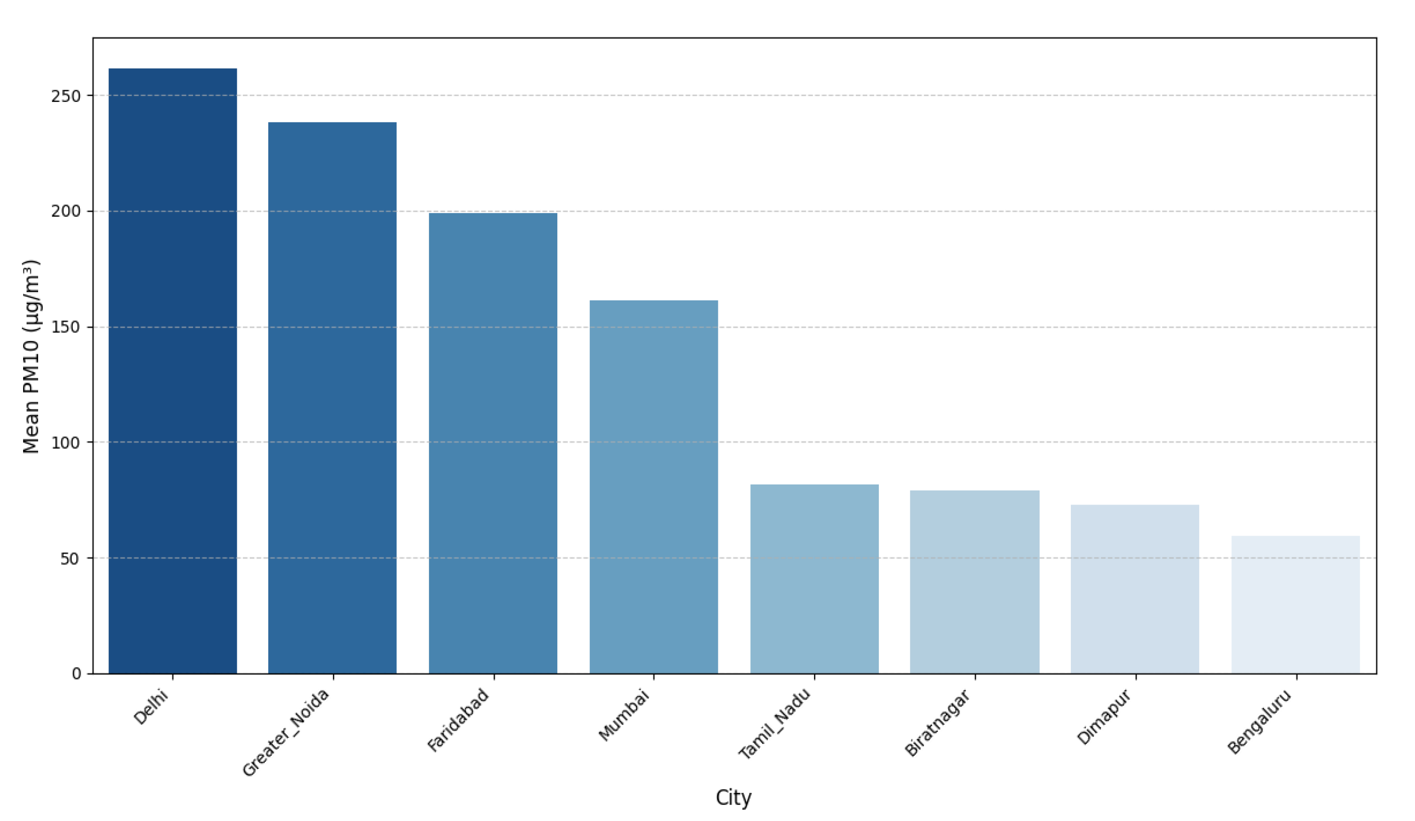
Figure 3 and Figure 4 rank the cities by their mean of PM 2.5 and PM 10 concentrations, highlighting the wide variance in pollution levels across the study region.

3.2. Data Acquisition and Pre-Processing

We used a publicly available Dataset, which is a collection of unique visual and quantitative environmental data of the Air Pollution Image Dataset from 7 cities in India and one city in Nepal, as reported by [53]. Multiple-scene 12,240 Images Figure 1, pre-categorized into six standard AQI classes (Good, Moderate, Unhealthy for Sensitive Groups, Unhealthy, Very Unhealthy, and Hazardous) given in Table 1. The corresponding tabular time-series data collected from the Central Pollution Control Board (CPCB) contain measurements of pollutants, including AQI, PM 2.5 , PM 10 , O 3 , CO, SO 2 and NO 2 .
We used AQI, PM 2.5 , and PM 10 in this study by linking each image to a relevant entry in the corresponding city based on its AQI class label. In the final dataset, each sample consists of an image associated with a tabular feature vector, and a label of ground-truth for each class. We split the dataset into training and testing into 80% and 20% respectively.
The two data modalities were pre-processed independently: In image pre-processing, all images were resized to a uniform dimension of 224 × 224 pixels and normalized by using the standard pre-processing function for the ResNet50 architecture. In the Tabular Pre-processing, features are scaled and transformed to have a mean of 0 and a standard deviation of 1, given in Equation (1).
z = x μ σ
Figure 5 illustrates the number of images available for each of the six AQI classes across the different cities in the dataset. shows the distribution of image samples across different cities and AQI classes. represents the seven cities, with the number of images available for each AQI class. corresponds to a specific AQI class: a_Good for a Low pollution, which is safe air quality. b_Moderate—is Acceptable air quality but pose risks for sensitive individuals.c_Unhealthy for Sensitive Groups which carry Risk increases for vulnerable groups including children, elderly, patients.d_Unhealthy—Hazardous for the general population. e_Very Unhealthy is Health warnings of emergency conditions and f_Severe is Extremely hazardous, emergency-level pollution. also illustrate that Delhi has the largest share of images in the Very Unhealthy and Severe categories, indicating critical air pollution. This distribution highlights significant city-level differences in AQI classes, emphasizing the imbalance of pollution levels across all cities and motivating the need for robust classification models.

3.3. The Vision-AQ Model Architecture

The Vision-AQ is a dual-branch multi-modal designed to fuse visual information from ground-level images with quantitative data synergistically. The architecture, as depicted in Figure 6, consists of two parallel processing streams that converge at a fusion point before making a final classification.
The primary role of the Image Branch is to act as the “eyes” of the model, extracting high-level visual features relevant to air quality. It utilizes a pre-trained ResNet50 model, with its weights initialized from ImageNet, as a powerful feature extractor. The input image 224   ×   224   ×   3 pixels passes through the convolutional base of the ResNet50. The resulting multi-dimensional feature map is then spatially summarized by a Global Average Pooling (GAP) layer.
V c = 1 H × W i = 1 H j = 1 W F i j c
For each feature map, the Global Average Pooling (GAP) layer calculates the mean of all spatial elements ( H × W ) . A single value V c is produced as described in Equation (2), where F i j c denotes the activation at spatial position ( i , j ) in channel c of the compact feature vector V image . The output of the GAP layer is then fed into a Dense layer to generate a compact Image Feature Vector, which is subsequently passed through another Dense layer to obtain a 64-dimensional representation of the image’s visual content. This representation encapsulates the salient visual information of the scene.
In the tabular branch, we use a Multi-Layer Perceptron (MLP) to process the scaled data. MLP consists of three sequential Dense layers with 64, 32, and 16 neurons, each employing the Rectified Linear Unit (ReLU) activation function defined in Equation (3). This produces a 16-dimensional feature vector capable of capturing non-linear relationships in complex patterns.
f ( x ) = max ( 0 , x )
The feature vectors from both branches, V image and V tabular , are concatenated at a fusion layer to form a single multi-modal representation:
V fused = V image V tabular
Here, ⊕ denotes the concatenation operation. The fused vector V fused is then passed through a Dense layer with 64 neurons and a ReLU activation function, followed by a Dropout layer with a rate of 0.5 for regularization. The final Dense layer employs a softmax activation function to produce a probability distribution over the K AQI classes. For a given output vector z, the probability of the i-th class is defined as:
σ ( z ) i = e z i j = 1 K e z j , i = 1 , , K
As shown in Table 2, the Vision-AQ model contains 13.9 million trainable parameters, while 23.6 million parameters are frozen from the ResNet50 backbone.

3.4. Training and Fine-Tuning Strategy

The Vision-AQ model is trained using the Adam optimizer to minimize the categorical cross-entropy loss function L, defined in Equation (6).
L ( y , y ^ ) = i = 1 K y i log ( y ^ i )
This loss function measures the dissimilarity between the true one-hot encoded label vector y and the model’s predicted probability distribution y ^ across all K classes.
The training process is conducted in two stages. In the first stage, feature extraction is performed with the ResNet50 backbone frozen, and only the newly added Dense layers are trained for 15 epochs. In the second stage, the model is fine-tuned by restoring the best weights, lowering the learning rate to 1 × 10 5 , and continuing training for an additional 10 epochs. This fine-tuning allows the specialized visual feature extractors to adapt subtly to the specific patterns of atmospheric haze and visibility present in the dataset. To prevent overfitting, Early Stopping and ModelCheckpoint callbacks are employed throughout training.

3.5. Grad-CAM

Gradient-weighted Class Activation Mapping (Grad-CAM) is a powerful explainable AI technique used to produce visual explanations for the decisions made by convolutional neural networks (CNNs) by generating heatmaps. Its primary purpose is to overcome the “black box” nature of deep learning models by highlighting the specific regions in an input image that are most important for a given prediction.
The Grad-CAM heatmap for a target class c is defined as in Equation (7):
L c Grad-CAM = ReLU k α c k A k
where A k is the k-th feature map in the final convolutional layer, and α c k is the gradient-based weight representing the importance of the k-th feature map for the target class c. The weight α c k is computed by global average pooling the gradients of the class score Y c with respect to the feature map A k . The term k α c k A k represents the weighted sum of all feature maps, and applying the ReLU function ensures that only the features positively influencing the target class are visualized.

4. Results

We present the performance of our proposed Vision-AQ model by analyzing its ability to predict air quality using different sources of data during training and validation In this section, as well as by applying XAI techniques to interpret its decision-making process for human understanding. The evaluation is structured to provide a comprehensive perspective on three key aspects: (i) the model’s generalization capability when applied to unseen test data, (ii) the effectiveness of its convergence during optimization, and (iii) the transparency and reliability of its predictions when examined through interpretable methods. By jointly considering performance metrics and interpretability analyses, this section not only demonstrates the predictive strength of Vision-AQ—through accuracy, precision, recall, and AUC scores—but also highlights the trustworthiness of its outputs. Such dual emphasis on performance and interpretability is critical for ensuring real-world applicability, as air quality monitoring systems must not only produce accurate results but also provide insights that can be validated and trusted by domain experts, policymakers, and the public.

4.1. Training Performance

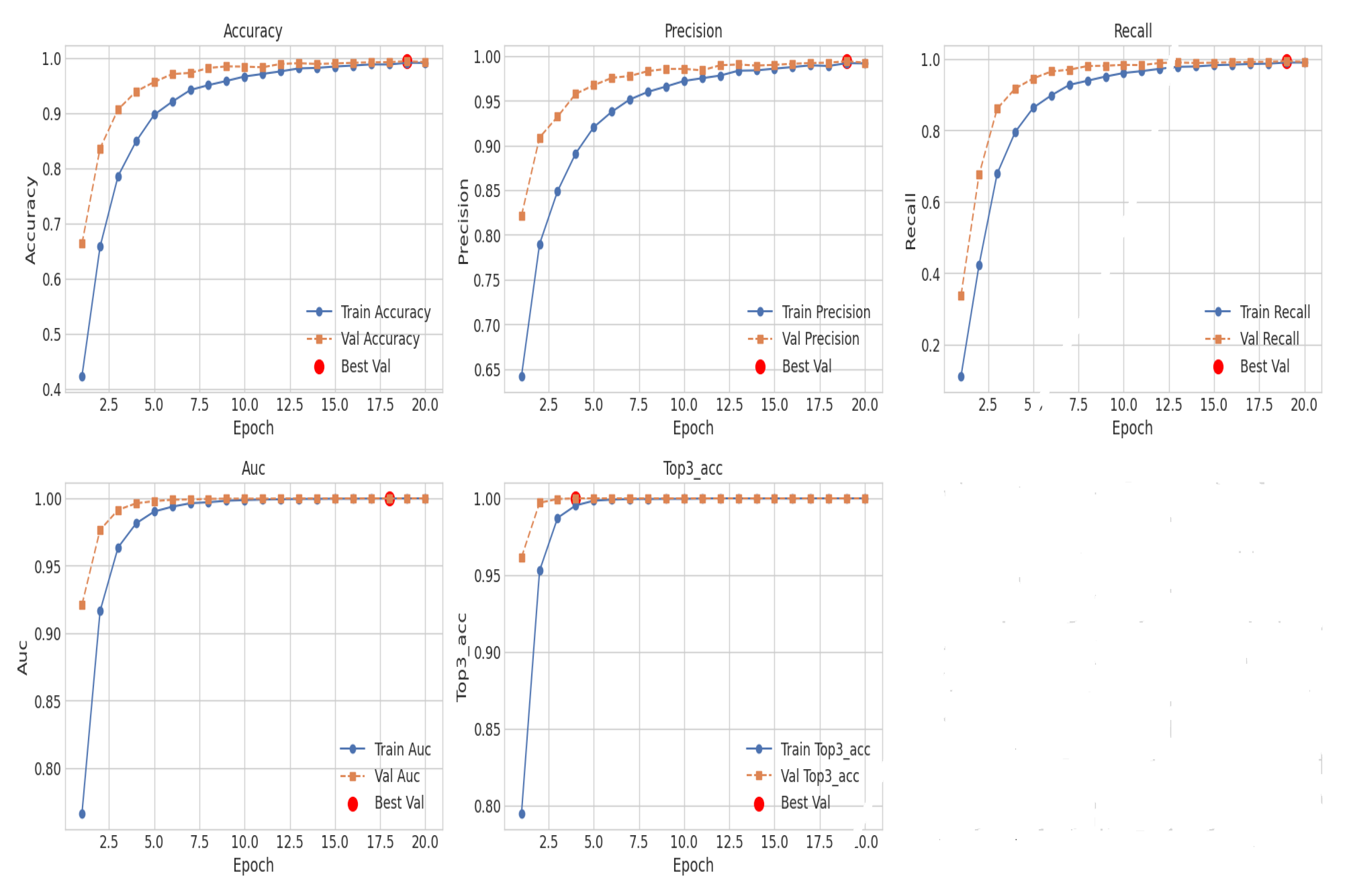
Vision-AQ model trained for 20 iterations. We monitored the performance metrics which illustrated in the training history of model and plots in Figure 7, which show the Accuracy, Precision, Recall, AUC, and Top-3 Accuracy for both the training and testing sets. The red marker indicates the point of best performance on the testing set.

4.2. Evaluation Metrics

The model’s performance is assessed by using a suite of standard classification metrics, including accuracy, given in Equation (8), precision by Equation (9), recall by Equation (10), F1-score by Equation (11), and a confusion matrix by Equation (12). Beyond performance, we also employed a comprehensive explainability framework to ensure the model’s decisions are transparent and trustworthy.
Recall = T P + T N T P + T N + F P + F N
Precision = T P T P + F P
Recall = T P T P + F N
F 1 - Score = 2 · Precision × Recall Precision + Recall
Confusion Matrix = T P F P F N T N
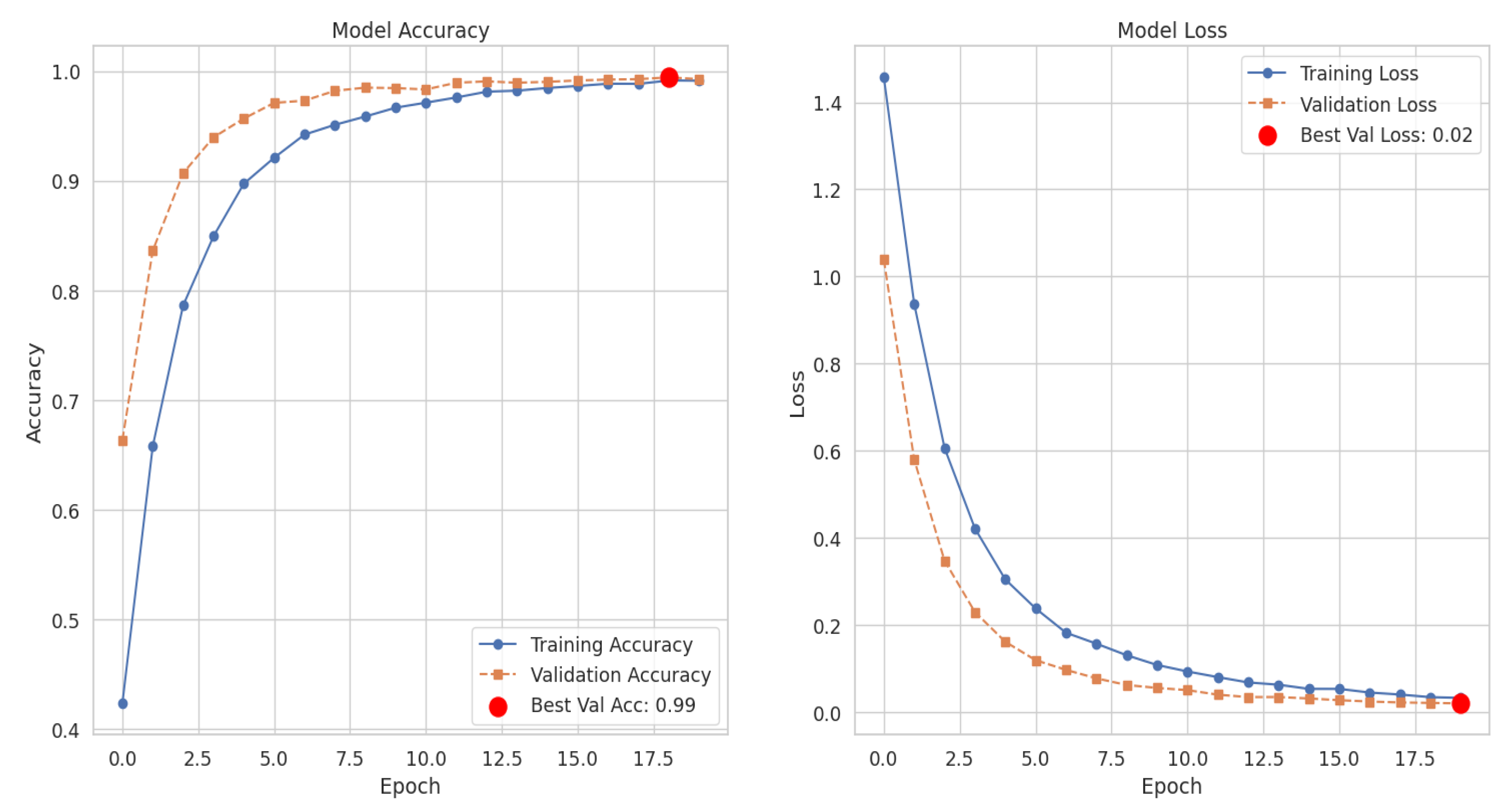
Learning curves. Figure 7 and Figure 8 show convergence in the first epochs, with all metrics, including accuracy, precision, and recall, increasing to optimal values. Training and testing curves track each other closely, indicating the model generalizes well to unseen data without significant overfitting. We use Early Stopping and Model Checkpoint, call backs to ensure that the model with the lowest testing loss is to be saved for final evaluation. The Vision-AQ model achieves the best testing accuracy, with similarly high performance across all monitored metrics.
Figure 8 Vision-AQ achieves the best testing accuracy of 99% and reaches the best testing loss of 0.02. The convergence of the curves demonstrates effective learning and good generalization. testing set, comprising 2448 image-tabular pairs in the test data set. The detailed per-class performance is given in the Classification Report in Table 3 of the Vision-AQ model.
Our Proposed Vision-AQ model demonstrates outstanding performance with an overall weighted average F1-score of 0.99 shown in the classification report in Table 3. Critically, the model achieves perfect precision and recall scores across all six AQI categories, from ’Good’ to ’Severe’. Performance indicates that the model is highly effective at distinguishing between different pollution levels.

4.3. Interpreting Predictions

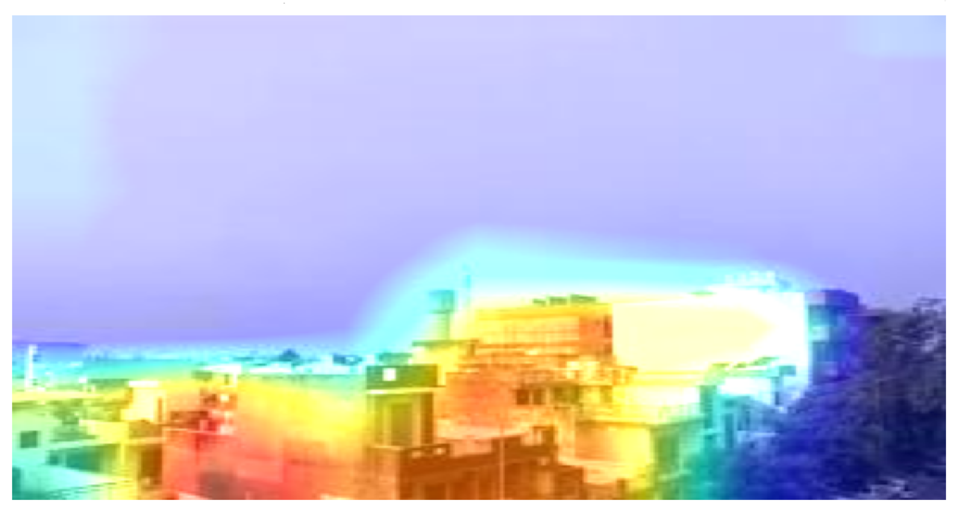
Figure 9 presents a Grad-CAM heatmap for an image correctly classified as Very Unhealthy. The activation map highlights yellow atmospheric haze and the obscured visibility of buildings in the background, with red regions indicating dense areas. This provides strong evidence that the CNN has learned to associate visual cues of aerosol scattering and reduced clarity with poor air quality, confirming that the model is focusing on relevant features for classification.
Figure 10 visualizes a misclassification where the image is labeled as Unhealthy for Sensitive Groups but mispredicted as Moderate. Grad-CAM highlights the areas that influenced the decision, showing attention on the brightly lit rooftop water tank and the clear blue sky rather than the subtle haze. This demonstrates that, under challenging conditions with mixed visual signals, the model can be distracted by salient but irrelevant features. Together, Figure 9 and Figure 10 illustrates that Grad-CAM provides interpretability by revealing the regions that contribute to both correct predictions and errors.

5. Discussion

Our proposed framework, Vision-AQ, demonstrates the strong potential of multi-modal deep learning for environmental sensing by achieving exceptional accuracy in AQI classification while also providing transparent, interpretable insights into its decision-making process. This section highlights the implications of our findings, situates them within existing literature, acknowledges the study’s limitations, and outlines future directions. The achieved F1-score of 0.99 underscores the effectiveness of our data fusion strategy, which integrates visual and tabular modalities. Unlike traditional approaches that analyze environmental data in isolation, Vision-AQ confirms that combining ground-level imagery with pollutant measurements yields a more holistic and robust understanding of air quality. Visual data captures contextual cues such as haze and reduced visibility, while quantitative sensor data anchors predictions in physical reality, reducing the risk of miss-classification.
A key contribution of this study is its emphasis on explainability. While the high predictive performance is noteworthy, the Grad-CAM visualizations provide deeper value by revealing that the model attends to scientifically relevant atmospheric features—such as smog and the obscuring of distant objects—when identifying poor air quality. This elevates the model from a “black box” to a trustworthy system whose logic can be validated. Our analysis of miss classifications further strengthens this contribution. Error visualizations revealed that the model occasionally focused on salient but irrelevant objects, providing a road-map for targeted improvements. For example, augmenting the dataset with more diverse lighting and environmental conditions could mitigate these weaknesses. The success of Vision-AQ has important implications for air quality management (AQM) in rapidly urbanizing regions. The framework demonstrates the feasibility of building dense networks of virtual sensors by leveraging low-cost, ubiquitous camera infrastructure to supplement expensive and sparsely distributed official monitoring stations. Such an approach could enable.
  • Real-time public health alerts via mobile applications.
  • Dynamic pollution maps to help citizens avoid hotspots.
  • Evidence-based urban planning informed by high-resolution environmental data.
Despite its strengths, this study has several limitations. The model was trained primarily on data from India and Nepal, and further evaluation is needed across diverse regions with varying meteorological and pollutant profiles. Additionally, the linkage between images and tabular data was constrained by broader AQI classes rather than precise timestamps, limiting opportunities for temporal modeling. Future research should expand the dataset to include more geographically diverse and temporally synchronized data. We also suggest in future work to deploy Vision-AQ in real-time to investigate advance data fusion methods and enhance robustness. We also acknowledge in limitation that PM 2.5 , PM 10 has direct optical manifestation in environmental imagery, as particles strongly influence light scattering and visibility. This is why the visual branch of Vision-AQ is most sensitive to particulate-driven pollution patterns such as haze and smog. However, the multi-modal design also incorporates tabular sensor data, which includes pollutants such as CO, SO 2 , and NO x in addition to PM 2.5 . While gases alone not produce strong visual cues detectable by the CNN, their concentrations are captured through the sensor-based MLP branch of our model. The fusion of visual and tabular features ensures that scenarios with low particulate levels but elevated gaseous pollutants are still appropriately classified. We clarify, that the visual pathway of Vision-AQ is not valid in invisible gases without PM 2.5 .

6. Conclusions

This study introduced Vision-AQ, an explainable multi-modal deep learning framework for air quality classification that integrates environmental imagery with pollutant data. The model achieved outstanding performance, with an F1-score of 0.99, and provided interpretable insights through Grad-CAM visualization, confirming its reliance on meaningful atmospheric features such as haze and reduced visibility. By combining the contextual richness of visual inputs with the precision of sensor data, Vision-AQ demonstrated the advantages of multi-modal data fusion over traditional single-modality approaches.
The framework offers a cost-effective and scalable solution for air quality monitoring, with potential applications in real-time public health alerts, pollution mapping, and urban policy support. While current assessment is limited to South Asian cities, future work will extend to diverse geographic regions, incorporate temporal modeling, and explore advanced fusion techniques. Ultimately, Vision-AQ represents a significant step toward explainable AI-driven environmental monitoring for smart cities.

Author Contributions

Conceptualization, F.M.; methodology, F.M.; software, F.M.; validation, S.U.R.; formal analysis, F.M.; investigation, S.U.R.; resources, A.C.; data curation, F.M.; writing—original draft preparation, F.M.; writing—review and editing, S.U.R. and A.C.; visualization, S.U.R.; supervision, A.C.; project administration, A.C.; funding acquisition, A.C. All authors have read and agreed to the published version of the manuscript.

Funding

This research was supported by a grant of the Korea Health Technology R&D Project through the Korea Health Industry Development Institute (KHIDI), funded by the Ministry of Health & Welfare, Republic of Korea (grant number: HI22C0646) and supported by the National Institute of Health (NIH) research project in South Korea (project No. 2024ER080300).

Data Availability Statement

The dataset we use in our study is publicly available at https://www.kaggle.com/datasets/adarshrouniyar/air-pollution-image-dataset-from-india-and-nepal (accessed on 1 October 2024).

Conflicts of Interest

The authors declare no conflict of interest.

References

  1. Zhao, L.; Li, Z.; Qu, L. A novel machine learning-based artificial intelligence method for predicting the air pollution index PM2.5. J. Clean. Prod. 2024, 468, 143042. [Google Scholar] [CrossRef]
  2. Dewage, P.M.; Wijeratne, L.O.; Yu, X.; Iqbal, M.; Balagopal, G.; Waczak, J.; Fernando, A.; Lary, M.D.; Ruwali, S.; Lary, D.J. Providing Fine Temporal and Spatial Resolution Analyses of Airborne Particulate Matter Utilizing Complimentary In Situ IoT Sensor Network and Remote Sensing Approaches. Remote Sens. 2024, 16, 2454. [Google Scholar] [CrossRef]
  3. Chakma, A.; Vizena, B.; Cao, T.; Lin, J.; Zhang, J. Image-based air quality analysis using deep convolutional neural network. In Proceedings of the 2017 IEEE International Conference on Image Processing (ICIP), Beijing, China, 17–20 September 2017; pp. 3949–3952. [Google Scholar]
  4. Essamlali, I.; Nhaila, H.; El Khaili, M. Supervised Machine Learning Approaches for Predicting Key Pollutants and for the Sustainable Enhancement of Urban Air Quality: A Systematic Review. Sustainability 2024, 16, 976. [Google Scholar] [CrossRef]
  5. Ćurić, M.; Zafirovski, O.; Spiridonov, V. Air quality and health. In Essentials of Medical Meteorology; Springer: Berlin/Heidelberg, Germany, 2021; pp. 143–182. [Google Scholar]
  6. Bayazid, A.B.; Jeong, S.A.; Azam, S.; Oh, S.H.; Lim, B.O. Neuroprotective effects of fermented blueberry and black rice against particulate matter 2.5 μm-induced inflammation in vitro and in vivo. Drug Chem. Toxicol. 2025, 48, 16–26. [Google Scholar] [CrossRef]
  7. Tang, Q.; Zhang, M.; Yu, L.; Deng, K.; Mao, H.; Hu, J.; Wang, C. Seasonal Dynamics of Microbial Communities in PM2.5 and PM10 from a Pig Barn. Animals 2025, 15, 1116. [Google Scholar] [CrossRef] [PubMed]
  8. Obodoeze, F.C.; Nwabueze, C.A.; Akaneme, S.A. Monitoring and prediction of PM2.5 pollution for a smart city. Int. J. Adv. Eng. Res. Sci 2021, 6, 181–185. [Google Scholar]
  9. Tham, H.P.; Yip, K.Y.; Aitipamula, S.; Mothe, S.R.; Zhao, W.; Choong, P.S.; Benetti, A.A.; Gan, W.E.; Leong, F.Y.; Thoniyot, P.; et al. Influence of particle parameters on deposition onto healthy and damaged human hair. Int. J. Cosmet. Sci. 2025, 47, 58–72. [Google Scholar] [CrossRef]
  10. Chauhan, A. Environmental Pollution and Management; Techsar Pvt. Ltd.: New Delhi, India, 2025. [Google Scholar]
  11. Mago, N.; Mittal, M.; Bhimavarapu, U.; Battineni, G. Optimized outdoor parking system for smart cities using advanced saliency detection method and hybrid features extraction model. J. Taibah Univ. Sci. 2022, 16, 401–414. [Google Scholar] [CrossRef]
  12. Huang, C.J.; Kuo, P.H. A deep CNN-LSTM model for particulate matter (PM2.5) forecasting in smart cities. Sensors 2018, 18, 2220. [Google Scholar] [CrossRef] [PubMed]
  13. Song, S.; Lam, J.C.; Han, Y.; Li, V.O. ResNet-LSTM for Real-Time PM2.5 and PM10 Estimation Using Sequential Smartphone Images. IEEE Access 2020, 8, 220069–220082. [Google Scholar] [CrossRef]
  14. Chen, S.; Kan, G.; Li, J.; Liang, K.; Hong, Y. Investigating China’s Urban Air Quality Using Big Data, Information Theory, and Machine Learning. Pol. J. Environ. Stud. 2018, 27, 565–578. [Google Scholar] [CrossRef] [PubMed]
  15. Bekkar, A.; Hssina, B.; Douzi, S.; Douzi, K. Air-pollution prediction in smart city, deep learning approach. J. Big Data 2021, 8, 161. [Google Scholar] [CrossRef]
  16. Njaime, M.; Abdallah, F.; Snoussi, H.; Akl, J.; Chaaban, K.; Omrani, H. Transfer learning based solution for air quality prediction in smart cities using multimodal data. Int. J. Environ. Sci. Technol. 2025, 22, 1297–1312. [Google Scholar] [CrossRef]
  17. Siddique, M.A.; Naseer, E.; Usama, M.; Basit, A. Estimation of Surface-Level NO2 Using Satellite Remote Sensing and Machine Learning: A review. IEEE Geosci. Remote Sens. Mag. 2024, 12, 8–34. [Google Scholar] [CrossRef]
  18. Mondal, S.; Adhikary, A.S.; Dutta, A.; Bhardwaj, R.; Dey, S. Utilizing Machine Learning for air pollution prediction, comprehensive impact assessment, and effective solutions in Kolkata, India. Results Earth Sci. 2024, 2, 100030. [Google Scholar] [CrossRef]
  19. Zhou, S.; Wang, W.; Zhu, L.; Qiao, Q.; Kang, Y. Deep-learning architecture for PM2.5 concentration prediction: A review. Environ. Sci. Ecotechnol. 2024, 21, 100400. [Google Scholar] [CrossRef]
  20. Chelani, A.; Rao, C.C.; Phadke, K.; Hasan, M. Formation of an air quality index in India. Int. J. Environ. Stud. 2002, 59, 331–342. [Google Scholar] [CrossRef]
  21. Holzinger, A.; Malle, B.; Saranti, A.; Pfeifer, B. Towards multi-modal causability with graph neural networks enabling information fusion for explainable AI. Inf. Fusion 2021, 71, 28–37. [Google Scholar] [CrossRef]
  22. Zhang, S.; Li, Y.; Mei, S. Exploring uni-modal feature learning on entities and relations for remote sensing cross-modal text-image retrieval. IEEE Trans. Geosci. Remote Sens. 2023, 61, 1–17. [Google Scholar] [CrossRef]
  23. Sagl, G.; Resch, B.; Blaschke, T. Contextual sensing: Integrating contextual information with human and technical geo-sensor information for smart cities. Sensors 2015, 15, 17013–17035. [Google Scholar] [CrossRef]
  24. Wang, S.; Mei, L.; Liu, R.; Jiang, W.; Yin, Z.; Deng, X.; He, T. Multi-modal fusion sensing: A comprehensive review of millimeter-wave radar and its integration with other modalities. IEEE Commun. Surv. Tutor. 2024, 27, 322–352. [Google Scholar] [CrossRef]
  25. Rai, A. Explainable AI: From black box to glass box. J. Acad. Mark. Sci. 2020, 48, 137–141. [Google Scholar] [CrossRef]
  26. Kumar, M.; Khan, L.; Choi, A. RAMHA: A Hybrid Social Text-Based Transformer with Adapter for Mental Health Emotion Classification. Mathematics 2025, 13, 2918. [Google Scholar] [CrossRef]
  27. Lauriks, T.; Longo, R.; Baetens, D.; Derudi, M.; Parente, A.; Bellemans, A.; Van Beeck, J.; Denys, S. Application of improved CFD modeling for prediction and mitigation of traffic-related air pollution hotspots in a realistic urban street. Atmos. Environ. 2021, 246, 118127. [Google Scholar] [CrossRef]
  28. Zhang, L.; Liu, Y.; Zhao, F. Important meteorological variables for statistical long-term air quality prediction in eastern China. Theor. Appl. Climatol. 2018, 134, 25–36. [Google Scholar] [CrossRef]
  29. Ashby, L.; Anderson, M. Studies in the politics of environmental protection: The historical roots of the British Clean Air Act, 1956: II. The appeal to public opinion over domestic smoke, 1880–1892. Interdiscip. Sci. Rev. 1977, 2, 9–26. [Google Scholar] [CrossRef]
  30. Stern, A.C.; Professor, E. History of air pollution legislation in the United States. J. Air Pollut. Control Assoc. 1982, 32, 44–61. [Google Scholar] [CrossRef] [PubMed]
  31. Schmalensee, R.; Stavins, R.N. Policy evolution under the clean air act. J. Econ. Perspect. 2019, 33, 27–50. [Google Scholar] [CrossRef]
  32. Snyder, H.R. Major depressive disorder is associated with broad impairments on neuropsychological measures of executive function: A meta-analysis and review. Psychol. Bull. 2013, 139, 81. [Google Scholar] [CrossRef]
  33. Dillon, L.; Sellers, C.; Underhill, V.; Shapiro, N.; Ohayon, J.L.; Sullivan, M.; Brown, P.; Harrison, J.; Wylie, S.; EPA Under Siege Writing Group. The Environmental Protection Agency in the early Trump administration: Prelude to regulatory capture. Am. J. Public Health 2018, 108, S89–S94. [Google Scholar] [CrossRef]
  34. Gupta, P.; Christopher, S.A.; Wang, J.; Gehrig, R.; Lee, Y.; Kumar, N. Satellite remote sensing of particulate matter and air quality assessment over global cities. Atmos. Environ. 2006, 40, 5880–5892. [Google Scholar] [CrossRef]
  35. Morawska, L.; Thai, P.K.; Liu, X.; Asumadu-Sakyi, A.; Ayoko, G.; Bartonova, A.; Bedini, A.; Chai, F.; Christensen, B.; Dunbabin, M.; et al. Applications of low-cost sensing technologies for air quality monitoring and exposure assessment: How far have they gone? Environ. Int. 2018, 116, 286–299. [Google Scholar] [CrossRef]
  36. Karagulian, F.; Temimi, M.; Ghebreyesus, D.; Weston, M.; Kondapalli, N.K.; Valappil, V.K.; Aldababesh, A.; Lyapustin, A.; Chaouch, N.; Al Hammadi, F.; et al. Analysis of a severe dust storm and its impact on air quality conditions using WRF-Chem modeling, satellite imagery, and ground observations. Air Qual. Atmos. Health 2019, 12, 453–470. [Google Scholar] [CrossRef]
  37. Northam, A.E. Development and Evaluation of a Model to Correct Tapered Element Oscillating Microbalance (TEOM) Readings of PM2.5 in Chullora, Sydney. Ph.D. Thesis, University of Wollongong, Wollongong, Australia, 2017. [Google Scholar]
  38. Trujillo, C. Evaluation of Sensor-Based Air Monitoring Networks in the US and Globally: Guidance for Urban Networks. Master’s Thesis, University of Illinois at Chicago, Chicago, IL, USA, 2025. [Google Scholar]
  39. Van Donkelaar, A.; Martin, R.V.; Brauer, M.; Kahn, R.; Levy, R.; Verduzco, C.; Villeneuve, P.J. Global estimates of ambient fine particulate matter concentrations from satellite-based aerosol optical depth: Development and application. Environ. Health Perspect. 2010, 118, 847–855. [Google Scholar] [CrossRef] [PubMed]
  40. Barnaba, F.; Putaud, J.P.; Gruening, C.; dell’Acqua, A.; Dos Santos, S. Annual cycle in co-located in situ, total-column, and height-resolved aerosol observations in the Po Valley (Italy): Implications for ground-level particulate matter mass concentration estimation from remote sensing. J. Geophys. Res. Atmos. 2010, 115. [Google Scholar] [CrossRef]
  41. Li, J. Pollution trends in China from 2000 to 2017: A multi-sensor view from space. Remote Sens. 2020, 12, 208. [Google Scholar] [CrossRef]
  42. Yu, X.; Wong, M.S.; Nazeer, M.; Li, Z.; Kwok, C.Y.T. A novel algorithm for full-coverage daily aerosol optical depth retrievals using machine learning-based reconstruction technique. Atmos. Environ. 2024, 318, 120216. [Google Scholar] [CrossRef]
  43. Liu, C.; Tsow, F.; Zou, Y.; Tao, N. Particle pollution estimation based on image analysis. PLoS ONE 2016, 11, e0145955. [Google Scholar] [CrossRef]
  44. Wan, H.; Xu, R.; Zhang, M.; Cai, Y.; Li, J.; Shen, X. A novel model for water quality prediction caused by non-point sources pollution based on deep learning and feature extraction methods. J. Hydrol. 2022, 612, 128081. [Google Scholar] [CrossRef]
  45. Zhou, C.; Zhou, C.; Zhu, H.; Liu, T. AIR-CNN: A lightweight automatic image rectification CNN used for barrel distortion. Meas. Sci. Technol. 2024, 35, 045402. [Google Scholar] [CrossRef]
  46. Zhang, Q.; Han, Y.; Li, V.O.; Lam, J.C. Deep-AIR: A hybrid CNN-LSTM framework for fine-grained air pollution estimation and forecast in metropolitan cities. IEEE Access 2022, 10, 55818–55841. [Google Scholar] [CrossRef]
  47. Zhang, C.; Yan, J.; Li, C.; Rui, X.; Liu, L.; Bie, R. On estimating air pollution from photos using convolutional neural network. In Proceedings of the 24th ACM international conference on Multimedia, Amsterdam, The Netherlands, 15–19 October 2016; pp. 297–301. [Google Scholar]
  48. Chen, H.; Chen, A.; Xu, L.; Xie, H.; Qiao, H.; Lin, Q.; Cai, K. A deep learning CNN architecture applied in smart near-infrared analysis of water pollution for agricultural irrigation resources. Agric. Water Manag. 2020, 240, 106303. [Google Scholar] [CrossRef]
  49. Ahmed, N.; Islam, M.N.; Tuba, A.S.; Mahdy, M.; Sujauddin, M. Solving visual pollution with deep learning: A new nexus in environmental management. J. Environ. Manag. 2019, 248, 109253. [Google Scholar] [CrossRef] [PubMed]
  50. Ahmed, M.; Shen, Y.; Ahmed, M.; Xiao, Z.; Cheng, P.; Ali, N.; Ghaffar, A.; Ali, S. AQE-Net: A deep learning model for estimating air quality of Karachi city from mobile images. Remote Sens. 2022, 14, 5732. [Google Scholar] [CrossRef]
  51. Bishoi, B.; Prakash, A.; Jain, V. A comparative study of air quality index based on factor analysis and US-EPA methods for an urban environment. Aerosol Air Qual. Res. 2009, 9, 1–17. [Google Scholar] [CrossRef]
  52. Bhawan, P.; Nagar, E.A. Central pollution control board. Cent. Pollut. Control Board New Delhi India Tech. Rep. 2020, 20–21. [Google Scholar]
  53. Rouniyar, A.; Utomo, S.; John, A.; Hsiung, P.A. Air Pollution Image Dataset from India and Nepal; Kaggle: San Francisco, CA, USA, 2023. [Google Scholar]
Figure 1. Representative sample images from the dataset.
Mathematics 13 03017 g001
Figure 2. Image count distribution by city and AQI class.
Mathematics 13 03017 g002
Figure 3. Average PM 2.5 concentration by city.
Mathematics 13 03017 g003
Figure 4. Average PM 10 concentration by city.
Mathematics 13 03017 g004
Figure 5. Image data distribution of AQI classes across cities.
Mathematics 13 03017 g005
Figure 6. Vision-AQ model architecture for air quality classification and visual interpretation.
Mathematics 13 03017 g006
Figure 7. Vision-AQ training metrics over epochs.
Mathematics 13 03017 g007
Figure 8. ViSION-AQ training and Testing history.
Mathematics 13 03017 g008
Figure 9. Grad-CAM for a correct prediction. The heatmap shows the model focusing on atmospheric haze to correctly identify the scene as ’Very Unhealthy’.
Mathematics 13 03017 g009
Figure 10. Grad-CAM for a Mi-classification. true label was un-healthy for sensitive group but model incorrectly predicts as ‘Moderate’ and focus on the clear sky and a bright object, overlook the subtle atmospheric haze.
Mathematics 13 03017 g010
Table 1. Classification of air quality based on selected pollutants of AQI, PM 2.5 and PM 10 from a comprehensive dataset.
Label ClassAQI PM 2.5 ( μ g/m 3 ) PM 10 ( μ g/m 3 )
Good0–500–120–54
Moderate51–10012.1–35.455–154
Unhealthy for Sensitive Groups101–15035.5–55.4155–254
Unhealthy151–20055.5–150.4255–354
Very Unhealthy201–300150.5–250.4355–424
Severe>300>250.4>424
Table 2. Model architecture summary of Vision-AQ.
Layer BlockDescriptionOutput ShapeParams
Inputs
image_inputImage input (224 × 224 × 3)(None, 224, 224, 3)0
tabular_inputSensor input (3 features)(None, 3)0
Image Branch
resnet50CNN base (frozen)(None, 7, 7, 2048)0
global_avg_poolFeature pooling(None, 2048)0
image_featuresDense layer (64-dim)(None, 64)131,136
Tabular Branch
MLP Layers64 → 32 → 16(None, 16)2800
Fusion & Classifier
feature_fusionConcat (image+tabular)(None, 80)0
classifier_denseDense (64)(None, 64)5184
classifier_dropoutDropout (0.5)(None, 64)0
outputDense (6, Softmax)(None, 6)390
Total Params:23,733,510
Trainable:139,510
Non-trainable:23,594,000
Table 3. Classification report of air quality category prediction.
ClassPrecisionRecallF1-ScoreSupport
a_Good0.990.970.98308
b_Moderate0.970.990.98315
c_Unhealthy_for_Sensitive_Groups1.001.001.00573
d_Unhealthy1.001.001.00524
e_Very_Unhealthy1.001.001.00439
f_Severe0.991.001.00289
Accuracy0.992448
Macro Avg0.990.990.992448
Weighted Avg0.990.990.992448
Disclaimer/Publisher’s Note: The statements, opinions and data contained in all publications are solely those of the individual author(s) and contributor(s) and not of MDPI and/or the editor(s). MDPI and/or the editor(s) disclaim responsibility for any injury to people or property resulting from any ideas, methods, instructions or products referred to in the content.