Extremely Optimal Graph Research for Network Reliability

Abstract

Network reliability refers to a probabilistic measure of a network system’s ability to maintain its intended service functionality within a specified time interval and under given operating conditions. Let $\Omega (n,m)$ be the set of all simple two-terminal networks on n vertices and m edges. If each edge operates independently with the same fixed probability $p\in [0,1]$, then the two-terminal reliability, denoted by $R_2(G,P))$, is the probability that there exists a path between two target vertices s and t. For a given number of vertices n and edges m, there are some graphs within $\Omega (n,m)$ that have higher reliability than others, and these are known as extremely optimal graphs. In this work, we determine the sets of extremely optimal graphs in two classes of two-terminal network with sizes $m={\displaystyle \frac{n(n-1))}{2}}-2$ and $m={\displaystyle \frac{n(n-1))}{2}}-3$, consisting of 2 and 5 networks, respectively. Moreover, we identify one class of graphs obtained by deleting some edges among non-target vertices in the complete two-terminal graph, and we count the number of graphs of this class with size ${\displaystyle \frac{n(n-1)}{2}}-\lfloor {\displaystyle \frac{n-2}{2}}\rfloor \le m\le {\displaystyle \frac{n(n-1))}{2}}-1$ by applying the Pólya counting principle.

1. Introduction

Network reliability refers to the probability that a network system maintains connectivity between specified nodes under given conditions, typically modeled using probabilistic graph theory that accounts for random failures of edges or nodes [1]. Primary evaluation approaches include exact analytical methods based on minimal path/cut sets, Monte Carlo simulation for large-scale networks, and graph-theoretical methods that identify optimal network configurations through extremal theory. This research provides a theoretical foundation for fault-tolerant network design and has significant application value in fields such as communication networks and distributed systems.

In the study of an optimal network based on extremal theory, the exploration of extremely optimal graphs holds significant theoretical value and application prospects. These graph structures can achieve the theoretical limits of network reliability under given constraints, providing benchmark references for the performance upper bounds in network design. Currently, research in this field remains in its infancy, having extremely limited existing results. The available literature focuses primarily on all-terminal reliability scenarios, which investigate the properties of extremal graphs that ensure connectivity among all the nodes in a network. However, there is a notable lack of systematic research on two-terminal reliability scenarios, which is a more practically valuable context in engineering applications. By advancing the study of extremely optimal graphs in two-terminal networks, this research will propel the expansion of network reliability theory from all-connected scenarios to more targeted point-to-point connectivity scenarios, carrying substantial academic innovation value and engineering application significance.

Let $G=\left(V\right(G),E(G\left)\right)$ be a two-terminal graph, where $V\left(G\right)$ is the vertex set and $E\left(G\right)$ is the edge set. An $st$-path set in the two terminal graph G is a set of edges in $E\left(G\right)$ that contains a path from the vertices s to t. In this work, we are only concerned with simple graphs. In fact, determining exact values for the size of an $st$-path set is a difficult problem [2,3].

The above model—a two-terminal graph—can be applied to observe the two-terminal reliability of a network. If each edge of such a graph operates independently with the same fixed probability $p\in [0,1]$, the two-terminal reliability, denoted by $R_2(G,P))$, is the probability that there exists a path between the target vertices. Much of the work in this field focuses on identifying bounds on the coefficients of two-terminal reliability polynomials [4,5,6]. A two-terminal graph $G\in \Omega (n,m)$ is said to be uniformly most reliable or uniformly optimal in $\Omega (n,m)$, if $R_2(G,p)\ge R_2(H,p)$ for all $p\in [0,1]$ and all H in $\Omega (n,m)$. However, a uniformly optimal graph does not always exist [7]. The problem of graph reliability is then considered from another perspective [8] by asking whether we can find an extremely optimal graph set in which the reliability of any other graph is less than that of each graph in this set for all $p\in [0,1]$. We must consider the existence of a uniformly optimal graph and the determination of an extremely optimal graph set. If such a graph exists, then it is clearly the only graph contained in the corresponding extremely optimal graph set. Much similar research has been performed [9,10,11,12,13].

For all-terminal graphs, Zhao [8] proved that when $n\ge 8$ was even, the cardinalities of the extremely optimal graph set for the graph family $\Omega (n,{\displaystyle \frac{n(n-1))}{2}}-{\displaystyle \frac{n+2}{2}})$ and $\Omega (n,{\displaystyle \frac{n(n-1))}{2}}-{\displaystyle \frac{n+4}{2}})$ were 2 and 6, respectively, and when $n\ge 8$ was odd, the cardinality of the extremely optimal graph set for the graph family $\Omega (n,{\displaystyle \frac{n(n-1))}{2}}-{\displaystyle \frac{n+3}{2}})$ was 4. In the case of two-terminal graphs, their extremely optimal graphs are different from those of all-terminal graphs. Two-terminal graphs have been used in real-world applications such as transportation networks [14,15,16,17], but there are few results on this topic.

In [18], the authors determined the uniformly optimal graph of the two-terminal network $\Omega (n,{\displaystyle \frac{n(n-1))}{2}}-1)$ and proved that, when ${\displaystyle \frac{n(n-1)}{2}}-\lfloor {\displaystyle \frac{n-2}{2}}\rfloor \le m\le {\displaystyle \frac{n(n-1))}{2}}-4$, there was no uniformly optimal graph in the corresponding network. In this work, we expand the study to extremely optimal graphs with the same conditions as above. In other words, utilizing the related theory of two-terminal graphs, extremely optimal graph sets are found for the cases of $m={\displaystyle \frac{n(n-1))}{2}}-2$ and $m={\displaystyle \frac{n(n-1))}{2}}-3$. Moreover, we determine a type of graph obtained by deleting some edges among non-target vertices in the complete two-terminal graph, and we apply the Pólya counting principle to count the number of graphs in this class with size ${\displaystyle \frac{n(n-1)}{2}}-12\le m\le {\displaystyle \frac{n(n-1))}{2}}-1$.

This study of extremely optimal networks provides novel theoretical perspectives and optimization pathways for the analysis of network reliability. These graph structures exhibit optimal reliability characteristics under specific constraints, enabling researchers to circumvent the challenge of seeking “universally optimal solutions”. By analyzing the topological properties of extremely optimal graphs, we can not only uncover the intrinsic principles of highly reliable networks but also develop actionable optimization frameworks for practical network design. Through rigorous mathematical proofs and extensive numerical experiments, this research systematically establishes the evaluation criteria and construction methods for extremely optimal graphs. The findings have significant guiding value for engineering practices such as survivability design in communication networks and redundancy configuration in power systems, particularly to improve the resilience of critical infrastructure against random failures and targeted attacks.

2. Existence of the Extremely Optimal Network

For any simple graph G with n vertices and m edges, the two-terminal reliability polynomial can be defined as

$$R_2(G,p)=\sum _{i=1}^m{N}_i{p}^i{(1-p)}^{m-i}$$

(1)

where $N_i$ is the number of $st$-path sets with size i in G for each $i\in \{1,2,\cdots ,m\}$, and $p\in [0,1]$ is the probability that its edges operate independently.

Definition 1

([8]). Let n and m be positive integers. If there are graphs $G_1,G_2,\cdots ,G_a$, such that $R\left(G_i,p\right)\ge R(G,p)$, for each $1\le i\le a$ and all G in $\Omega (n,m)$, then $G_1,G_2,\cdots ,G_a$ is an extremely optimal graph set of $\Omega (n,m)$.

For simplicity, if the graphs $G,H\in \Omega (n,m)$ satisfy $R(G,p)>R(H,p)$, then denote this by $G\succ H$.

Definition 2

([18]). Let $n\ge 4$ and $m={\displaystyle \frac{n(n-1))}{2}}-1$ be positive integers.

1 

Define $X_n$ as the two-terminal graph on n vertices and m edges with vertex set $V\left(X_n\right)=\left\{s=x_1,x_2,\cdots ,x_n=t\right\}$, and edge set $E\left(X_n\right)=\left\{x_i{x}_j:1\le i<j\le n\right\}\setminus \left\{st\right\}$;

2 

Define $Y_n$ as the two-terminal graph on n vertices and m edges with vertex set $V\left(Y_n\right)=\left\{s=y_1,y_2,\cdots ,y_n=t\right\}$, and edge set $E\left(Y_n\right)=\left\{y_i{y}_j:1\le i<j\le n\right\}\setminus \left\{s{y}_2\right\}$;

3 

Define $Z_n$ as the two-terminal graph on n vertices and m edges with vertex set $V\left(Z_n\right)=\left\{s=z_1,z_2,\cdots ,z_n=t\right\}$, and edge set $E\left(Z_n\right)=\left\{z_i{z}_j:1\le i<j\le n\right\}\setminus \left\{z_2{z}_3\right\}$.

The above three graphs are shown in Figure 1, where the red edges represent the deleted edges, and the blue edges represent the independently operable edges, and the Figure 2, Figure 3, Figure A1 and Figure A2 in the following text represent the same meaning. Furthermore, the pseudo-code for the algorithm of network two-terminal reliability is provided in Appendix A.

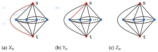
Figure 1. Graphs $X_n$, $Y_n$, and $Z_n$.

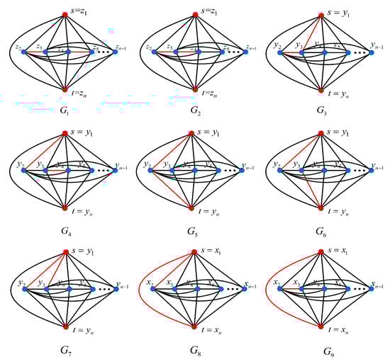
Figure 2. All cases of graph family $\Omega (n,{\displaystyle \frac{n(n-1))}{2}}-2)$.

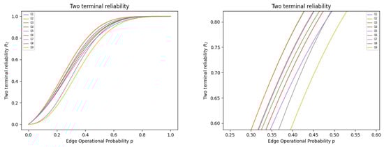
Figure 3. In the figure, the one on the left shows Two-terminal reliabilities for graphs $G_1,G_2,\cdots G_9$ in the case of $n=6,m=13$; the one on the right represents its partial enlargement of the left one.

As previously noted, when removing two or three edges from a complete graph, there is no uniformly optimal graph in the graph family $\Omega (n,m)$ [5]. Based on the above case, the existence of the extremely optimal graphs and the determination of the minimal extremely optimal graph set will be considered as follows.

Theorem 1

([18]). Let $n\ge 8$ and $2\le r\le \lfloor {\displaystyle \frac{n(n-1))}{2}}\rfloor$ be positive integers. If $m={\displaystyle \frac{n(n-1))}{2}}-r$, then there is no uniformly most reliable two-terminal graph in $\Omega (n,m)$.

To determine the existence of an extremely optimal graph in a graph family $\Omega (n,m)$ is mainly to analyze the reliability of graphs globally on the interval $[0,1]$. The reliability of each graph in the extremely optimal graph set is greater than that of any other graph in the same graph family. Later, we analyze the extremely optimal graph sets of two graph families with $m={\displaystyle \frac{n(n-1))}{2}}-2$ and $m={\displaystyle \frac{n(n-1))}{2}}-3$.

Now, we classify all graphs into $\Omega (n,m)$ according to three types:

• In an $X_n$-type graph, the edge $st$ and the other $r-1$ edges are deleted;
• In a $Y_n$-type graph, the r edges between the target vertex and non-target vertices are deleted;
• In a $Z_n$-type graph, the r edges between the non-target vertices are deleted.

Theorem 2.

Let $n\ge 6$ be a positive integer and $m={\displaystyle \frac{n(n-1))}{2}}-2$. Then there are two extremely optimal graphs in $\Omega (n,m)$.

Proof of Theorem 2.

We can construct all the non-isomorphic subgraphs obtained by removing two edges from an n-order complete two-terminal graph, as shown in Figure 2. Based on the above classification, we have the following: $Z_n$-type graphs contain $G_1$ and $G_2$; $Y_n$-type graphs contain $G_3$, $G_4$, $G_5$, $G_6$, and $G_7$; $X_n$-type graphs contain $G_8$ and $G_9$.

To prove that a $Z_n$-type graph is more reliable than any one of the $X_n$-type and $Y_n$-type graphs, we show that there are more $st$-path sets with size $k(1\le k\le m)$ in $Z_n$-type graphs than in $X_n$-type graphs and $Y_n$-type graphs by constructing an injection from the $st$-path sets of size k in $X_n$-type and $Y_n$-type graphs to the $st$-path sets of size k in a $Z_n$-type graph. Thus, we consider the following two cases.

Case 1. A $Z_n$-type graph is more reliable than an $X_n$-type graph. Without loss of generality, we prove that $G_1\succ G_8$.

Let $V\left(X_n\right)=V\left(G_8\right)$, $E\left(X_n\right)=E\left(G_8\right)$, $V\left(Z_n\right)=V\left(G_1\right)$, and $E\left(Z_n\right)=E\left(G_1\right)$. Now construct an injection ${\phi }_1$ from the $st$-path sets of size k in $X_n$ to the $st$-path sets of size k in $Z_n$. Let P be the $st$-path sets of size k in $X_n$. The following two sub-cases are considered.

Subcase 1.1. Suppose P does not contain an edge $x_4{x}_5$. Then set ${\phi }_1\left(P\right)=\left\{z_i{z}_j\right|x_i{x}_j\in P\}$. Note that the image is an $st$-path set in $Z_n$ with the same size as P that does not contain edge $st$.

Subcase 1.2. Suppose P contains edge $x_4{x}_5$. Then define ${\phi }_1\left(P\right)=\left\{z_i{z}_j\right|x_i{x}_j\in P\}\bigcup \left\{st\right\}\setminus \left\{z_4{z}_5\right\}$. Note that the image is an $st$-path set in $Z_n$ with the same size as P that contains edge $st$, which is distinct from that in subcase 1.1.

Then ${\phi }_1$ is an injection and there are at least as many $st$-path sets in $Z_n$ as in $X_n$. Thus is uniformly more reliable than $X_n$, i.e., $G_1\succ G_8$. Similarly, $G_i\succ G_j$, $i=1,2$ and $j=8,9$.

Case 2. A $Z_n$-type graphs is more reliable than a $Y_n$-type graph. Without loss of generality, we can prove that $G_2\succ G_3$.

Let $V\left(Y_n\right)=V\left(G_3\right)$, $E\left(Y_n\right)=E\left(G_3\right)$, $V\left(Z_n\right)=V\left(G_2\right)$ and $E\left(Z_n\right)=E\left(G_2\right)$. We construct a mapping ${\phi }_2$ from an $st$-path sets of k in $Y_n$ to an $st$-path sets of k in $Z_n$. Let P be an $st$-path sets of size $1\le k\le m$ in $Y_n$. We discuss four sub-cases.

Subcase 2.1. Suppose $P\setminus \left\{y_3{y}_4\right\}$ does not contain edge $y_3{y}_4$. Then let ${\phi }_2\left(P\right)=\left\{z_i{z}_j\right|y_i{y}_j\in P\}$. The image is an $st$-path sets in $Z_n$ with the same size as P, which does not contain edge $s{z}_3$.

Subcase 2.2. Suppose P contains edge $y_3{y}_4$ and $P\setminus \left\{y_3{y}_4\right\}$ is still an $st$-path sets. Then define ${\phi }_2\left(P\right)=\left\{z_i{z}_j\right|y_i{y}_j\in P\}\cup \left\{s{z}_3\right\}\setminus \left\{z_3{z}_4\right\}$. The image is an $st$-path sets in $Z_n$ with the same size as P which contains edge $s{z}_3$. We can see that ${\phi }_2\left(P\right)\setminus \left\{s{z}_3\right\}$ is still an $st$-path sets.

Subcase 2.3. Suppose P contains edge $y_3{y}_4$ and $P\setminus \left\{y_3{y}_4\right\}$ is not an $st$-path sets but it is a $y_{3}t$-path-set. Then define ${\phi }_2\left(P\right)=\left\{z_i{z}_j\right|y_i{y}_j\in P\}\cup \left\{s{z}_3\right\}\setminus \left\{z_3{z}_4\right\}$. Note that the image is an $st$-path sets in $Z_n$ with the same size as P, which contains the edge $s{z}_3$. Evidently, ${\phi }_2\left(P\right)\setminus \left\{s{z}_3\right\}$ is not an $st$-path sets which is distinct from any one of the images in subcase 2.2.

Subcase 2.4. Now suppose P contains edge $y_3{y}_4$, $P\setminus \left\{y_3{y}_4\right\}$ is not an $st$-path sets and it is also not a $y_{3}t$-path-set. Then define

${\phi }_2\left(P\right)=\left\{z_i{z}_j\right|2\le i\le j\le n,y_i{y}_j\in P\}\cup \left\{z_4{z}_j\right|s{y}_j\in P\}\cup \left\{s{z}_3\right\}\setminus \left\{z_3{z}_4\right\}$.

Note that ${\phi }_2\left(P\right)$ has the same size as P, which is completely disjoint from the image described in subcase 2.3. Since the mapping ${\phi }_2$ defined in both of these two cases yields disjoint $st$-path sets of $Z_n$, it is an injection. Then, there are at least as many $st$-path sets of size k in $Z_n$ as in $Y_n$, and $Z_n$ is uniformly more reliable than $Y_n$. That is, $G_2\succ G_3$.

Similarly, $G_i\succ G_j$, $i=1,2$ and $j=3,4,5,6,7$.

Thus, we find that graphs $G_1$ and $G_2$ are uniformly more reliable than other graphs in $\Omega (n,{\displaystyle \frac{n(n-1))}{2}}-2)$, which are just the $Z_n$-type graphs.    □

In Figure 3, we plot the two-terminal reliabilities for graphs $G_1,G_2,\cdots G_9$ in the case of $n=6,m=13$.

In Figure 3, we clearly see that the curves corresponding to $G_1$ and $G_2$ are at the top. Furthermore, we consider the case of removing three edges from a complete two-terminal graph, which will appear as more non-isomorphic subgraphs. However, the extremely optimal graphs can still be found in the same way. Therefore, we obtain Theorem 3.

Theorem 3.

Let $n\ge 8$ be a positive integer and $m={\displaystyle \frac{n(n-1))}{2}}-3$. Then there are five extremely optimal graphs in $\Omega (n,m)$.

Proof of Theorem 3.

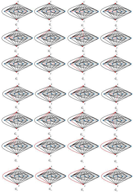
All the non-isomorphic graphs obtained by removing three edges from an n-order complete two-terminal graph can be constructed, as shown in Figure 4. We have:

Figure 4. All cases of graph family $\Omega (n,{\displaystyle \frac{n(n-1))}{2}}-3)$.

$Z_n$-type graphs containing $G_1$, $G_2$, $G_3$, $G_4$,$G_5$;

$Y_n$-type graphs containing $G_6$–$G_{21}$;

$X_n$-type graphs containing $G_{22}$–$G_{28}$.

We can also construct two injections from the $st$-path sets of size k $(1\le k\le m)$ in $X_n$-type and $Y_n$-type graphs to $st$-path sets of size k in $Z_n$-type graphs.

Case 1. A $Z_n$-type graph is more reliable than an $X_n$-type graph. Without loss of generality, we prove that $G_3\succ G_{22}$.

Let $V\left(X_n\right)=V\left(G_{22}\right)$, $E\left(X_n\right)=E\left(G_{22}\right)$, $V\left(Z_n\right)=V\left(G_3\right)$ and $E\left(Z_n\right)=E\left(G_3\right)$. We construct an injection ${\theta }_1$ from an $st$-path sets of size k in $X_n$ to the $st$-path sets of size k in $Z_n$. Let Q be the $st$-path sets of size k in $X_n$. We consider two subcases.

Subcase 1.1. Suppose Q does not contain edge $x_4{x}_5$. Then let ${\theta }_1\left(Q\right)=\left\{z_i{z}_j\right|x_i{x}_j\in Q\}$. Note that the image is an $st$-path sets in $Z_n$ with the same size as Q, which does not contain edge $st$.

Subcase 1.2. Suppose Q contains edge $x_4{x}_5$. Then define ${\theta }_1\left(Q\right)=\left\{z_i{z}_j\right|x_i{x}_j\in Q\}\cup \left\{st\right\}\setminus \left\{z_4{z}_5\right\}$. The image is an $st$-path sets in $Z_n$ with the same size as Q, which contains the edge $st$. Thus, the image is distinct from those in subcase 1.1.

Then ${\theta }_1$ is an injection and there are at least as many $st$-path sets in $Z_n$ as in $X_n$. Thus, $Z_n$ is uniformly more reliable than $X_n$, i.e., $G_3\succ G_{22}$. We can prove the following results analogous to the proof of Theorem 2. It holds that $G_i\succ G_j$, $i=1,2,4,5$ and $j=23,24,\cdots ,28$.

Case 2. A $Z_n$-type graph is more reliable than a $Y_n$-type graph. In this case, without loss of generality, we prove that $G_4\succ G_7$.

Let $V\left(Y_n\right)=V\left(G_7\right)$, $E\left(Y_n\right)=E\left(G_7\right)$, $V\left(Z_n\right)=V\left(G_4\right)$, and $E\left(Z_n\right)=E\left(G_4\right)$. We construct a mapping ${\theta }_2$ from an $st$-path set of k in $Y_n$ to an $st$-path set of k in $Z_n$. Let Q be the $st$-path set of size $1⩽k⩽m$ in $Y_n$. We discuss four sub-cases.

Subcase 2.1. Suppose Q does not contain edge $y_4{y}_5$. Then let ${\theta }_2\left(Q\right)=\left\{z_i{z}_j\right|y_i{y}_j\in Q\}$. Note that the image is the $st$-path set in $Z_n$ with the same size as Q, which does not contain edge $s{z}_4$.

Subcase 2.2. Suppose Q contains edge $y_4{y}_5$, and $Q\setminus \left\{y_4{y}_5\right\}$ is still an $st$-path set. Then define ${\theta }_2\left(Q\right)=\left\{z_i{z}_j\right|y_i{y}_j\in Q\}\cup \left\{s{z}_4\right\}\setminus \left\{z_4{z}_5\right\}$. The corresponding image is the $st$-path set in $Z_n$ with the same size as Q, which contains edge $s{z}_4$. We can see that ${\theta }_2\left(Q\right)\setminus \left\{s{z}_4\right\}$ is still an $st$-path set.

Subcase 2.3. Suppose Q contains edge $y_4{y}_5$ and that $P\setminus \left\{y_4{y}_5\right\}$ is not an $st$-path set, but it is a $y_{4}t$-path-set. Then define ${\theta }_2\left(Q\right)=\left\{z_i{z}_j\right|y_i{y}_j\in Q\}\cup \left\{s{z}_4\right\}\setminus \left\{z_4{z}_5\right\}$. Note that the image consists of the $st$-path sets in $Z_n$, with the same size as Q, which contain the edge $s{z}_4$, but ${\theta }_2\left(Q\right)\setminus \left\{s{z}_4\right\}$ is not an $st$-path set, which is distinct from the image in subcase 2.2.

Subcase 2.4. Now suppose Q contains edge $y_4{y}_5$, and $P\setminus \left\{y_4{y}_5\right\}$ is not an $st$-path set and it is not a $y_{4}t$-path-set. Then define

${\theta }_2\left(Q\right)=\left\{z_i{z}_j\right|2\le i<j\le n,y_i{y}_j\in Q\}\cup \left\{z_5{z}_j\right|s{y}_j\in Q\}\cup \left\{s{z}_4\right\}\setminus \left\{z_4{z}_5\right\}$.

Note that ${\theta }_2\left(Q\right)$ has the same size as Q, and it is completely disjoint from the image described in subcase 2.3.

In each of the above four subcases, ${\theta }_2$ yields disjoint $st$-path sets of $Z_n$. Then the mapping is an injection. There are at least as many $st$-path sets of size k in $Z_n$ as in $Y_n$, and hence $Z_n$ is uniformly more reliable than $Y_n$, i.e., $G_4\succ G_7$. We can similarly prove that $G_i\succ G_j$, $i=1,2,3,5$, and $j=6,8,9,\cdots ,21$.

In summary, we can find that graphs $G_1$, $G_2$, $G_3$, $G_4$, and $G_5$ are uniformly more reliable than other graphs, constitute the minimum extremely optimal graph set in the graph family $\Omega (n,{\displaystyle \frac{n(n-1)}{2}}-3)$, and are exactly the $Z_n$-type graphs.    □

For better visualization, in Figure 5 we plot two-terminal reliabilities for the graphs $G_1,G_2,\cdots G_{28}$ in the case of $n=8,m=25$.

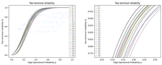
Figure 5. The left figure shows the two-terminal reliability curve for graphs $G_1,G_2,\cdots G_{28}$ in the case of $n=8$, $m=25$, while the right figure represents its partial enlargement.

Referring to Theorems 2 and 3, it is evident that $Z_n$-type graphs exhibit higher uniform reliability than the other two types of graph in $\Omega (n,m)$, as more edges are deleted. Moreover, we can find that the number of extremely optimal graphs in their corresponding graph classes is constant as n keeps increasing.

3. The Number of Extremely Optimal Networks

It is easy to see that a $Z_n$-type graph is formed by deleting r($1\le r\le ⌊{\displaystyle \frac{n-2}{2}}⌋$) edges among non-target vertices for the complete two-terminal graph $K_n$, which is equivalent to the simple graph obtained by deleting any r edges in the complete graph $K_{n-2}$ with $n-2$ non-target vertices.

Let N be the number of non-isomorphic subgraphs of the complete two-terminal graph $K_n$. We can visualize the relationship between r and N in logarithmic coordinates and fit the corresponding curves, as shown in Figure 6. Then we can see that, as the parameter r increases, the number of non-isomorphic subgraphs N grows exponentially. This work aims to reduce the search range for more reliable graphs. Then it is sufficient to count the number of a specific type of graphs, i.e., $Z_n$-type graphs. In the following, we apply the Pólya counting principle to count the parameter N by deleting the edges of $1\le r\le 12$.

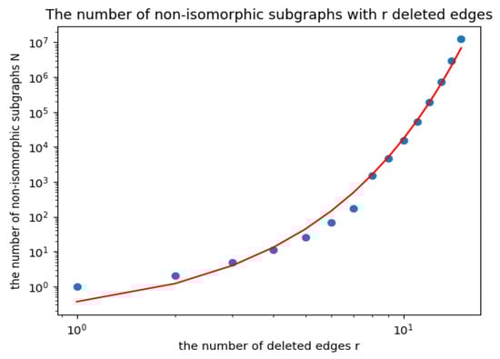
Figure 6. The relationship between r and N in logarithmic coordinates and their curve fitting.

Lemma 1.

(Pólya theorem for generating function type) Let n objects be colored with m colors $b_1,b_2,\cdots ,b_m$ and n objects to form a permutation group $G=\{a_1,a_2,\cdots ,a_g\}$, where $a_i=1^{k_{i_1}}{2}^{k_{i_2}}{3}^{k_{i_3}}\cdots n^{k_{i_n}}$ and $k_{i_j}$ denotes the number of rotations of j order in the permutation $a_i$. Then the Pólya theorem for generating function type is as follows.

$$P={\displaystyle \frac{1}{\left|G\right|}}\left[{\sum _{i=1}^g\prod _{j=1}^n\left({b_1}^j+{b_2}^j+\cdots +{b_m}^j\right)}^{k_{i_j}}\right],$$

(2)

where the coefficients of ${b_1}^{k_1}{b_2}^{k_2}\cdots {b_m}^{k_m}$ indicate the numbers of coloring schemes in which there are $k_i$ objects with color $b_i$, $1\le i\le m$.

If the edges of $K_n$ are colored by two colors $b_1$ and $b_2$, then the number of different schemes is the number of its spanning subgraphs, which is equivalent to enumeration polynomials in the Pólya theorem in the case of $b_1=r=x,b_2=b=1$.

Next, we calculate the number of $Z_n$-type graphs as deleting 2 and 3 edges and take complete two-terminal graphs of order 8 as an example. Clearly, we only need to calculate the number of spanning subgraphs of $K_6$ (See Figure 7 and Table 1).

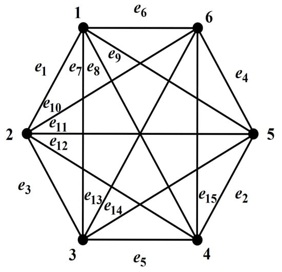
Figure 7. $K_6$.

Table 1. Enumeration of non-isomorphic subgraphs of $K_6$.

Group ${\mathit{S}}_6$	Permutation of the Corresponding Edges	Number	Type
$\left(1\right)\left(2\right)\left(3\right)\left(4\right)\left(5\right)\left(6\right)$	e	1	$1^{15}$
$\left(135\right)\left(246\right)$	$\left(e_1{e}_5{e}_4\right)\left(e_2{e}_6{e}_3\right)\left(e_7{e}_{14}{e}_9\right)\left(e_8{e}_{13}{e}_{11}\right)\left(e_{10}{e}_{12}{e}_{15}\right)$	40	$3^5$
$\left(12\right)\left(36\right)\left(45\right)$	$\left(e_3{e}_6\right)\left(e_4{e}_5\right)\left(e_7{e}_{10}\right)\left(e_8{e}_{11}\right)\left(e_9{e}_{12}\right)\left(e_{14}{e}_{15}\right)$	15	$1^3{2}^6$
$\left(12\right)\left(3\right)\left(4\right)\left(5\right)\left(6\right)$	$\left(e_3{e}_7\right)\left(e_6{e}_{10}\right)\left(e_8{e}_{12}\right)\left(e_9{e}_{11}\right)$	15	$1^7{2}^4$
$\left(1234\right)\left(5\right)\left(6\right)$	$\left(e_1{e}_3{e}_5{e}_8\right)\left(e_2{e}_9{e}_{11}{e}_{14}\right)\left(e_4\right)\left(e_6{e}_{10}{e}_{13}{e}_{15}\right)\left(e_7{e}_{12}\right)$	90	$1^1{2}^1{4}^3$
$\left(123\right)\left(4\right)\left(5\right)\left(6\right)$	$\left(e_1{e}_3{e}_7\right)\left(e_5{e}_8{e}_{12}\right)\left(e_6{e}_{10}{e}_{13}\right)\left(e_9{e}_{11}{e}_{14}\right)\left(e_{15}\right)$	40	$1^3{3}^4$
$\left(12345\right)\left(6\right)$	$\left(e_1{e}_3{e}_5{e}_2{e}_9\right)\left(e_4{e}_6{e}_{10}{e}_{13}{e}_{15}\right)\left(e_7{e}_{12}{e}_{14}{e}_8{e}_{11}\right)$	144	$5^3$
$\left(1\right)\left(23\right)\left(456\right)$	$\left(e_1{e}_7\right)\left(e_2{e}_4{e}_{15}\right)\left(e_5{e}_{11}{e}_{13}{e}_{12}{e}_{14}{e}_{10}\right)\left(e_6{e}_8{e}_9\right)$	120	$1^1{2}^1{3}^2{6}^1$
$\left(12\right)\left(3456\right)$	$\left(e_2{e}_4{e}_{13}{e}_5\right)\left(e_3{e}_8{e}_{11}{e}_6\right)\left(e_7{e}_{12}{e}_9{e}_{10}\right)\left(e_{14}{e}_{15}\right)$	90	$1^1{2}^1{4}^3$
$\left(123456\right)$	$\left(e_1{e}_3{e}_5{e}_2{e}_4{e}_6\right)\left(e_7{e}_{12}{e}_{14}{e}_{15}{e}_9{e}_{10}\right)\left(e_8{e}_{11}{e}_{13}\right)$	120	$3^1{6}^2$
$\left(13\right)\left(2\right)\left(46\right)\left(5\right)$	$\left(e_1{e}_3\right)\left(e_2{e}_4\right)\left(e_5{e}_6\right)\left(e_8{e}_{13}\right)\left(e_9{e}_{14}\right)\left(e_{10}{e}_{12}\right)$	45	$1^3{2}^6$

As $n=6,7,8$, if $b_1=r=x,b_2=b=1$, then

$\begin{array}{cc}\hfill P_6\left(x\right)& ={\displaystyle \frac{1}{720}}[{(x+1)}^{15}+40{(x^3+1)}^5+15{(x+1)}^3{(x^2+1)}^6+15{(x+1)}^7{(x^2+1)}^4+\hfill \\ & 90(x+1)(x^2+1){(x^4+1)}^3+40{(x+1)}^3{(x^3+1)}^4+144{(x^5+1)}^3+120(x+1)\hfill \\ & (x^2+1){(x^3+1)}^2(x^6+1)+90(x+1)(x^2+1){(x^4+1)}^3+120{(x^3+1)}^3\hfill \\ & {(x^6+1)}^2]\hfill \\ & =1+x+2x^2+5x^3+9x^4+15x^5+21x^6+24x^7+24x^8+21x^9+15x^{10}+9x^{11}\hfill \\ & +5x^{12}+2x^{13}+x^{14}+x^{15}\hfill \end{array}$

Similarly, we have

$\begin{array}{cc}\hfill P_7\left(x\right)& =1+x+2x^2+5x^3+10x^4+21x^5+41x^6+65x^7+97x^8+131x^9+148x^{10}+\hfill \\ & 148x^{11}+131x^{12}+97x^{13}+65x^{14}+41x^{15}+21x^{16}+10x^{17}+5x^{18}+2x^{19}+x^{20}+\hfill \\ & x^{21},\hfill \end{array}$

$\begin{array}{cc}\hfill P_8\left(x\right)& =1+x+2x^2+5x^3+11x^4+24x^5+56x^6+115x^7+221x^8+402x^9+663x^{10}+\hfill \\ & 980x^{11}+1312x^{12}+1557x^{13}+1646x^{14}+1557x^{15}+1312x^{16}+980x^{17}+663x^{18}+\hfill \\ & 402x^{19}+221x^{20}+115x^{21}+56x^{22}+24x^{23}+11x^{24}+5x^{25}+2x^{26}+x^{27}+x^{28}.\hfill \end{array}$

We see that the coefficients of the terms with exponents 2 and 3 are 2 and 5, respectively, which is consistent with Theorems 2 and 3. Table 2 gives the number of $Z_n$-type graphs for $1\le r\le 12$. Additionally, we provide pseudo-code for Pólya’s counting principle in Appendix A (See Algorithm A2).

Table 2. The number of the $Z_n$-type graphs for $1\le r\le 12$.

r	1	2	3	4	5	6	7	8	9	10	11	12
N	1	2	5	11	26	68	177	1476	4613	15,216	52,944	193,367

From the above, the determination of extremely optimal graphs is useful to find consistently more reliable graphs in the same graph family. From Table 2, we see that the number of $Z_n$-type graphs shows exponential growth as r increases.

However, for any r, there is a minimal subset of extremely optimal graphs, which is included in the set of the corresponding $Z_n$-type graphs.

4. Conclusions

The study of extremely optimal networks holds unique value for network reliability optimization. These special network structures reveal the theoretical upper bounds of reliability under resource constraints, providing benchmark references for practical network design. By analyzing the topological characteristics of extremal graphs, critical vulnerability points in networks can be identified to guide targeted reinforcement. This research avoids the computational complexity challenges inherent in traditional reliability analysis, offering new perspectives for evaluating reliability in large-scale network systems, with significant application potential in data center networks and IoT scenarios, etc.

In this paper, we studied the locally most reliable graphs in two special two-terminal graph families in which there are no uniformly optimal graphs. In particular, $Z_n$-type graphs are uniformly more reliable than $X_n$- and $Y_n$-type graphs under the same conditions. By classifying and comparing graphs, we proved the existence of an extremely optimal graph set, which plays an important role in constructing the most reliable graphs. Furthermore, the Pólya counting theorem was used to enumerate the number of $Z_n$-type graphs, which provided quantifiable design principles and optimization pathways for building highly robust networks. Its value extends beyond improving communication efficiency and resource utilization.

References

- Colbourn, C.J. The Combinatorics of Network Reliability; Oxford University Press: Oxford, UK, 1987. [Google Scholar]
- Brown, J.; Cox, D. Nonexistence of optimal graphs for all terminal reliability. Networks 2013, 63, 146–153. [Google Scholar] [CrossRef]
- Kelmans, A.K. On graphs with randomly deleted edges. Acta. Math. Acad. Sci. Hung. 1981, 37, 77–88. [Google Scholar] [CrossRef]
- Brecht, T.B.; Colbourn, C.J. Lower bounds on the two-terminal network reliability. Discrete Appl. Math. 1998, 21, 185–198. [Google Scholar] [CrossRef]
- Harms, D.D.; Colbourn, C.J. Renormalization of two-terminal reliability. Networks 1993, 23, 289–297. [Google Scholar] [CrossRef]
- Van Slyke, R.M.; Frank, H. Network reliability analysis: Part I. Networks 1972, 1, 279–290. [Google Scholar] [CrossRef]
- Myrvold, W.; Cheung, K.H.; Page, L.B.; Perry, J.E. Uniformly-most reliable networks do not always exist. Networks 1991, 21, 417–429. [Google Scholar] [CrossRef]
- Zhao, H.X. Research on Subgraph Polynomials and Reliability of Networks. Doctoral Dissertation, Northwestern Polytechnical University, Xi’an, China, 2004. [Google Scholar]
- Bauer, D.; Boesch, F.; Suffel, C.; Tindell, R. Combinatorial optimization problems in the analysis and design of probabilistic networks. Networks 1985, 15, 257–271. [Google Scholar] [CrossRef]
- Boesch, F.T.; Li, X.; Suffel, C. On the existence of uniformly optimal networks. Networks 1991, 21, 181–194. [Google Scholar] [CrossRef]
- Byer, O.D. Two path extremal graphs and an application to a Ramsey-type problem. Discrete Math. 1999, 196, 51–64. [Google Scholar] [CrossRef][Green Version]
- Romero, P. Uniformly optimally reliable graphs: A survey. Networks 2021, 80, 466–481. [Google Scholar] [CrossRef]
- Gross, D.; Saccoman, J.T. Uniformly optimal graphs. Networks 1998, 31, 217–225. [Google Scholar] [CrossRef]
- Shao, F.M.; Zhao, L.C. Optimal design improving a communication networks reliability. Microelectron Reliab. 1997, 37, 591–595. [Google Scholar] [CrossRef]
- Bobylev, D.A.; Borovskikh, L.P. A universal converter for the parameters of multicomponent two-terminal networks. Autom. Remote Control 2016, 77, 1649–1655. [Google Scholar] [CrossRef]
- Bai, G.; Zuo, M.J.; Tian, Z. Search for all d-MPs for all d levels in multistate two-terminal networks. Reliab. Eng. Syst. Saf. 2015, 142, 300–309. [Google Scholar] [CrossRef]
- Ibe, A.O.; Cory, B.J. Traveling Wave-based Fault Locator for Two and Three Terminal Networks. IEEE Trans. Power Syst. 1986, 1, 283–288. [Google Scholar] [CrossRef]
- Bertrand, H.; Goff, O.; Graves, G.; Sun, M. On uniformly most reliable two-terminal graphs. Networks 2018, 72, 200–216. [Google Scholar] [CrossRef]
Disclaimer/Publisher’s Note: The statements, opinions and data contained in all publications are solely those of the individual author(s) and contributor(s) and not of MDPI and/or the editor(s). MDPI and/or the editor(s) disclaim responsibility for any injury to people or property resulting from any ideas, methods, instructions or products referred to in the content. |
© 2025 by the authors. Licensee MDPI, Basel, Switzerland. This article is an open access article distributed under the terms and conditions of the Creative Commons Attribution (CC BY) license (https://creativecommons.org/licenses/by/4.0/).