Abstract
The generalized extreme value (GEV) distribution has been extensively applied in predicting extreme events across diverse fields, enabling accurate estimation of extreme quantiles of maxima. Although the mean and variance of the GEV can be expressed as functions of its parameters, a reparameterization that directly uses the mean and standard deviation as parameters provides interpretative advantages. This is particularly useful in regression-based models, as it allows a more straightforward interpretation of how covariates influence the mean and the standard deviation of the data. The proposed models are estimated within the Bayesian framework, assuming normal prior distributions for the regression coefficients. In this work, we introduce a reparameterization of the GEV distribution in terms of the mean and standard deviation, and apply it to minimum humidity data from the northeast region of Brazil. The results highlight the benefits of the proposed methodology, demonstrating clearer interpretability and practical relevance for extreme value modeling, where the influence of seasonal and locality variables on the mean and variance of minimum humidity can be accurately assessed.
Keywords:
Bayesian inference; extreme value theory; generalized extreme value distribution; mean and standard deviation modelling; parameterization MSC:
62F15; 62G32
1. Introduction
In recent decades, the need to study and predict extreme events has increased substantially. To address this demand, extreme value theory has emerged, offering more specific and sophisticated models capable of handling a wide range of problems. Several studies, such as [1,2], argue that climate change has intensified the occurrence of extreme events, leading to a noticeable rise in their frequency and impact over the years.
In recent decades, the study and prediction of extreme events have become increasingly relevant, given their impacts on society, the environment, and the economy. Extreme value theory has emerged as a key framework to address this challenge, providing specific and robust models that can be adapted to different types of problems. Several works, such as [1,2], point out that climate change has intensified the frequency and severity of extreme events, reinforcing the importance of accurate statistical modeling. Within this context, developing methodologies that improve both the estimation and interpretation of extremes is crucial, especially in applications where understanding the effect of covariates on the mean and variability of the data is essential, such as in climate studies and socioeconomic analyses.
According to [3], low humidity values can compromise photosynthesis and dry matter production, thereby affecting leaf area growth and impairing stomatal conductance. Beyond agricultural impacts, in order to characterize the levels of humidity that may pose risks to health and society, the Center for Meteorological and Climatic Research Applied to Agriculture (Cepagri) developed a psychometric scale. This scale assists authorities in determining the level of concern associated with a given humidity condition and supports decision-making for mitigating the effects of critically low humidity. Table 1 presents the classification established by this scale.

Table 1.
Psychrometric scale of air humidity criticality levels.
Studying the behavior of extreme low humidity is of great importance, as it enables authorities to adopt preventive measures and reduce the impacts that such events impose on society. Within extreme value theory, one of the most widely applied approaches is the analysis of block maxima. This method consists of dividing the data into blocks of size n and modeling the distribution of the maximum within each block. According to [4,5], regardless of the distribution of the observations within the block, the distribution of the block maxima converges to the generalized extreme value (GEV) distribution, with the cdf given by
defined on the set , where is the location parameter, is the scale parameter, and is the shape parameter. The parameter determines the tail weight of the distribution; when positive, it indicates that the data exhibit a heavy tail, suggesting a higher frequency of extreme values. Thus, for , the expression given for the cumulative distribution function is valid for , while for it is valid for . In the first case, at the lower end-point, it equals 0; in the second case, at the upper end-point, it equals 1. For , the expression given for the cdf is formally undefined and is replaced by the result obtained by taking the limit as . The sub-families of distributions defined by and correspond, respectively, to the Gumbel, Fréchet, and Weibull families of distributions. The probability density function (pdf) corresponding to (1) is
The values of the extreme quantiles of the block maxima distribution can then be obtained by inverting Equation (1), given by
where . Since it has a closed-form expression, quantile estimates can be obtained by substituting the parameter estimates into Equation (3). In extreme value analysis, the quantile is commonly referred to as the return level associated with the return period , and is interpreted as the value expected to be exceeded at least once within that period. This information provides a direct measure of the risk of an extreme event for the variable under study, allowing authorities and stakeholders to evaluate potential impacts and plan appropriate preventive measures.
The expected mean and variance associated with (1) are given by (for )
and
where is the Gamma function. In practice, is frequently assumed to be lower than 0.5, and the distribution has finite mean and variance. These measures are extremely important to measure the central tendency and variability of the GEV distribution.
Regression Models on Mean and Dispersion Parameters
Regression models are typically constructed to model the mean and/or dispersion of a distribution. In this context, the authors in ref. [6] proposed new parameterizations for the Birnbaum–Saunders distribution. One of them allows us to rely the Birnbaum–Saunders distribution on the mean. Recently, the authors in ref. [7] discussed a version of the inverse Gaussian model parameterized in terms of the mean and variance. Refs. [8,9,10] proposed new parameterizations of the inverse gamma beta prime and Pareto distributions in terms of a mean and a precision parameter. The authors also proposed the regression models based on their parameterizations of these distributions. Recently, the authors in refs. [11,12] extended the usual mean gamma and beta regression models using a general and unified parameterization of these distributions that is indexed by some central tendency measure, such as median, mode, arithmetic mean, geometric mean or harmonic mean, and a concentration parameter.
However, these mentioned models consider a regression structure only on the mean or on the mean and a dispersion parameter (but not variance). The interpretation of the dispersion parameter is only possible for fixed values of the mean. Hence, in all the models cited above, the variance is not explicitly modeled in terms of the explanatory variables. The authors in ref. [13] proposed a new parameterization for the beta distribution in terms of mean and variance for modeling bounded data. The authors in ref. [14] developed the novel parameterized IGPS class of distributions in terms of the mean and variance parameters.
In the context of extreme values, the authors in ref. [15] performed a reparameterization in the Generalized Pareto distribution as a function of the mean and dispersion of excesses, applied to maximum and minimum temperature data in the United States and Brazil, providing a direct interpretation of how geographic covariates, such as latitude, altitude, and month of the year, influence the mean and variance of minimum temperature. These covariates may also affect other environmental variables, such as minimum humidity, which serves as the focus of the present study. However, in spite of all these studies, not much attention has been paid to parameterizations of the three parameter GEV distribution that differ from those originally proposed by [4,5] based on the extreme events. The authors in ref. [16] considered quantile regression models to the maxima using the GEV distribution, considering a dynamic regression structure. In this way, it was possible to identify the direct effect of the covariates on the extreme quantiles of the observations. In this study, we adopt an approach in which the primary focus is to quantify the effect of covariates on the mean and variance.
Despite the superior properties of the GEV, its location, shape, and scale parameters do not directly correspond to the mean and dispersion, which complicates the interpretation of regression models specified using the GEV. Nevertheless, to the best of our knowledge, a regression model incorporating a structure for separate mean and variance parameters, similar to the normal regression model, has not yet been considered in the literature for modeling extreme values. The parameters of regression models for the mean and standard deviation are more readily interpretable than those of the location, shape, and scale parameters.
Thus, in this paper, we propose a novel parameterization of the GEV distribution in terms of the mean and standard deviation. In the context of minimum humidity data, it is important not only to capture the average value, which characterizes the central tendency of the distribution, but also to understand the variability and dispersion of the observations. Under this reparameterization, we introduce a regression framework that allows a separate regression structure for both the mean and the standard deviation parameters. In the proposed model, variations in the standard deviation can be directly interpreted in terms of changes in the explanatory variables. Parameter estimation is carried out within the Bayesian paradigm, providing a coherent probabilistic framework for uncertainty quantification and inference.
The rest of this study is organized as follows: Section 2 will present the proposed GEV distribution, reparameterized as a function of the mean and standard deviation. A structure of regression models for the parameters of this new model will also be presented. The Bayesian inference procedure is presented in Section 3. Section 4 presents an application of the proposed distribution, which consists in minimum humidity data in cities in the northeast region of Brazil. Section 5 presents the main conclusions of this work.
2. Regression Models Based on the Parametrization of the GEV Distribution by Its Mean and Standard Deviation
In this section, motivated by the need to directly estimate the expected value and variance of the extreme value distribution, we propose a reparameterized version of the GEV distribution in which the mean and standard deviation serve as parameters. Consider the parameterization where and are, respectively, the mean and variance of the GEV distribution given in (4) and (5) and written by
Let . Then we can write and in terms of , , and as follows:
By expressing the parameters and in terms of the mean and variance , and substituting these expressions into the cumulative distribution function in (1), the resulting reparameterized GEV distribution functions, for are given by
The density is obtained by differentiating the function (7), as follows:
For , the expression given for the cumulative distribution function is valid for , while for , it is valid for .
We use the notation to indicate that X is a random variable following a reparameterized GEV with mean and standard deviation parameter . Given that the arguments of the gamma function must be strictly positive, it is necessary to impose the condition on the shape parameter to ensure the existence of both the mean and the variance. We note that this parameterization was not proposed in the statistical literature.
Figure 1 illustrates the density curve of the proposed distribution in different scenarios. Increasing makes the curve the same, slightly shifted to the right, while increasing makes the curve flatter, and the mode value decreases.
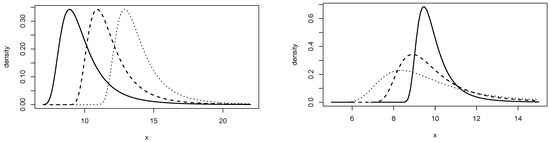
Figure 1.
Density of RGEV distribution in different scenarios. (Left): , , and varying in 10 (full), 12 (dashed), and 14 (dotted). (Right): , , and varying in 1 (full), 2 (dashed), and 3 (dotted).
Similarly, the quantile function can be written by inverting the cumulative distribution function in (7), and (for )
Regression Structure on the RGEV Parameters
Now, let be n independent random variables, where each , , follows the pdf given in (8). In order to introduce a regression structure in the RGEV parameters, we assume that
where , , and are vectors of unknown regression coefficients, which are assumed to be functionally independent, , , and , with , , , and are the linear predictors, and , , and are observations on , and m known-regressors, for . Furthermore, we assume that the covariate matrices , and have rank , and m, respectively.
Considering the parameter space of the RGEV distribution, the link function can be written as follows:
The proposed link functions are similar to those used in [16]. Since we use the canonical link function for , the coefficients represent the increase in the mean associated with a one-unit increase in the covariate. For , a one-unit increase in the covariate corresponds to an increase of in the logarithm of the standard deviation. In this reparametrization, for the parameter, in order to ensure the finiteness of the mean and variance, we shall impose the constraint in the inference procedure presented in the next section.
3. Bayesian Inference to the Proposed Model
3.1. Prior and Posterior Distribution
Considering a sample with distribution function, as in (7), the likelihood function is given by
For the proposed model, as the parameters are the values associated with each of the parameters, we will propose normal distributions for these parameters considering vague priors for them. In this way, we have that the priors for the parameters of the reparameterized GEV distribution will be defined as follows: and for ; and for ; and for , with . Note that the intercept represents the value of the parameter when all covariates are equal to zero; that is, it would be the value of the parameter if there was no regression structure. Furthermore, the intercepts have a normal distribution, whose mean is a value that represents the magnitude of the data that will be analyzed and may vary according to the application.
Assuming independent prior distributions for the coefficients in each predictor, their respective joint prior densities are expressed as
with .
As there is not much information on the true values of the parameters, a very common case in Bayesian inference, the prior distributions are chosen in such a way that they represent this lack of knowledge; in other words, the scale and location hyperparameters are normally adopted with high variance.
Using the prior distributions described in the previous section and the likelihood given in (9), the posterior joint density is proportional to
When examining the posterior distribution, it does not correspond to the analytical form of any standard distribution. Consequently, closed-form expressions for point and interval estimators of the parameters are not available, thereby requiring the use of numerical approximation techniques. In this study, Markov Chain Monte Carlo (MCMC) methods were employed [17].
3.2. MCMC Algorithm
Considering the posterior distribution in (10), the parameters of the RGEV distribution are sampled using the Metropolis–Hastings algorithm in blocks. In this scheme, the values of each of the three parameters are updated as separate blocks: in the first block, we sample , in the second block, , and in the third block, . The procedure for sampling the regression parameters follows a similar approach to that proposed by [18,19], and can be summarized as follows:
At the s-th iteration, the chains of the parameters move to step according to the following scheme:
- SamplingFor each , , sample from . The proposed vector together with does not yield a positive likelihood function in (9), so a new is sampled from . When the condition is satisfied, update with probability , where
- SamplingFor each , , sample from . The proposed vector together with does not yield a positive likelihood function in (9), so a new is sampled from . When the condition is satisfied, update with probability , where
- SamplingFor each , , sample from . The proposed vector together with does not yield a positive likelihood function in (9), so a new is sampled from . When the condition is satisfied, update with probability , where
The algorithm was implemented using the R statistical software [20], version 4.3. A total of 40,000 MCMC iterations were run, of which the first 10,000 were discarded as burn-in. From the remaining 30,000 iterations, every 100th draw was retained to form the posterior sample. Convergence of the algorithm was assessed by running two parallel chains with different initial values [17].
4. Applications to Real Data
The analyzed database consists of monthly minimum humidity in 109 monitoring stations in the northeast region of Brazil. As is standard in the analysis of extreme values, particularly when employing the Generalized Extreme Value (GEV) distribution, the modeling is typically performed on block maxima rather than minima. In order to analyze minimum humidity, we apply a transformation of the form , such that the maxima of the transformed variable x correspond to the minima of the original humidity values. Estimates of the mean and lower quantiles in the original scale can then be obtained by applying the inverse transformation.
For the choice of the covariates of the parameters , and , as we have 109 monitoring stations spread over a large region of the map, we consider that latitude () and altitude () may influence humidity. We used the standardized measures of these two variables in order to avoid distortions arising from differences in magnitude between the covariates. The mean and standard deviation of latitude were 8.64 and 3.63, respectively. For altitude, the mean and standard deviation were 284.49 and 236.33, respectively. Another location variable that can have a major influence on humidity is distance from the ocean. Cities close to the ocean have higher humidity levels and cities farther away are not affected by the sea. Thus, we define a binary variable () where the distance from the city to the coast is less than k kilometers, and otherwise.
To determine which value of the k cut-off point would be suitable for classifying the city as close to or far from the ocean, a graphical analysis of the dispersion of humidity in cities by distance was performed. Figure 2 shows the graph with the humidity for the months of January and July. From the graph, we can see that cities up to 25 km away from the sea have similar behavior, with higher humidity. Cities with more than 25 km of distance have behavior with lower humidity. Thus, we consider a suitable cut-off point to define the variable .
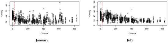
Figure 2.
Scatter plot of humidity in cities according to distance from the sea (in quilometers).
In addition to the effect of the geographic location of the city, as the minimum humidity levels were collected on a monthly basis, another covariate to be considered in this analysis is the effect of the month of the year, which can typically be captured using trigonometric functions, as was done, for example, in [18]. Thus, we also consider the covariates and , where m is the month.
Table 2 shows the estimation of model parameters, with respective 95% credibility intervals (CIs). Regarding the mean , when analyzing , it is noted that it is not significant, indicating that latitude does not influence the mean humidity. For the , the presence of significant and positive correlation is noted, with this we can say that the altitude has an influence on the average humidity. The point estimate of this parameter, , indicates that for every 236 m above sea level, humidity decreases by 1.25%. This behavior is also present in , indicating that cities near the sea have, on average, a 15.16% higher humidity than in coastal cities. Finally, we have and , which are also significant, but has a positive correlation, and a negative correlation. Thus, we can say that the months of the year also influence the mean humidity.
Table 2.
Estimates and CIs with respect to the parameters.
Regarding the parameter , Table 2 shows that, for , there is a significant negative relationship. This shows that cities at lower latitudes have greater variations in humidity. For each one-degree decrease in latitude, the average humidity is expected to be 1.16% higher. In , the same behavior is observed as in . Therefore, it is possible to conclude that the altitude also has an influence on the dispersion of humidity, so that the higher the altitude, the smaller the dispersion of the humidity data. More specifically, each 236 m increase in altitude is associated with an expected reduction in the standard deviation of humidity of = 1.05%. In sequence, we have , which is also significant, with the distance from the ocean having a negative influence on the standard deviation. The standard deviation of humidity in non-coastal cities is greater than that observed in coastal cities. Finally, we have and , which are also significant, in contrast to what was observed for the parameter, this time has a positive correlation, and has a negative correlation. Therefore, it can be said that the months of the year also influence the dispersion of the humidity.
Considering the parameter , we have , which has a positive association. Therefore, it can be said that latitude influences the shape of the distribution. In , a negative association is observed. Therefore, it is possible to state that altitude also has a certain influence on the form of data distribution. In sequence, we have , which also has significance arising from a negative association. With this, it is concluded that the distance to the sea influences the form of data distribution. Finally, we have and , which are also significant, showing that the months of the year also influence the way in which the data are distributed.
Figure 3 shows the graph of the behavior of the mean and standard deviation of the minimum air humidity in relation to the months of the year in the city of Teresina-PI. Firstly, it is noticed that the amplitude of the average values of humidity varies between 24% and 34%, characterizing a variation between the state of attention and the state of observation of the psychrometric scale (Table 1). After that, it is observed that the highest averages of humidity are present in the months of March, April, and May. On the other hand, the lowest averages observed are present in the months of September, October, and November. In general, it is noted that, considering the course of 1 year, the average humidity shows an increasing trend from January to April. From April, it begins to have a fall that runs until October, where the values increase again. Regarding the standard deviation, the months that show the greatest variability are May and June, and those with a smaller dispersion are November and December.
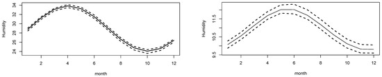
Figure 3.
Mean and standard deviation of minimum humidity in the city of Teresina-PI over the months. Lines represent a posteriori median and limits of the 95% CI.
Spatial Analysis of Humidity
In order to generally visualize the behavior of the minimum air humidity in the entire northeast region of Brazil, we made a map of the estimates obtained for the parameters considering an ordinary kriging [21], which is a classical geostatistical interpolation method used to predict the value of a spatially distributed variable at unsampled locations.
Figure 4 presents the average of minimum humidity for the northeast for some months of the year. In general, it is clear that cities near the coast have higher humidity than cities in the interior of the northeast. In addition, the interior region of Bahia stands out for having the lowest humidity. Regarding the months of the year, we see that January and July have similar behaviors, where most cities have an average humidity between 20% and 30%. In addition, it is observed that, among the months presented, April is the one with the highest humidity, whereas October is the driest month, as the average in most locations reaches below 20%.
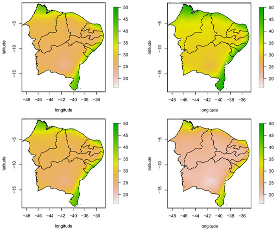
Figure 4.
Map for the mean minimum relative humidity in the stations of Northeast Brazil. (Top): January (left) and April (right). (Bottom): July (left) and October (right).
Figure 5 shows the variability of the minimum relative humidity in the northeast region in relation to some months of the year. In general, the greatest variability is present in the months of April and July. In addition, it is observed that the coastal regions have greater variability than the interior regions of the northeast. In January and October, the variability has similar behavior, but is lower than July and April.
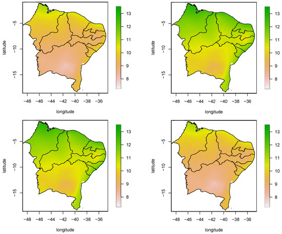
Figure 5.
Map for the dispersion of the minimum humidity of the air in the stations of the northeast of Brazil. (Top): January (left) and April (right). (Bottom): July (left) and October (right).
Figure 6 shows the posterior median of the 5% quantile in some months. The month of April has the highest humidity values, as it can be seen that, for almost the entire northeast region, the humidity values are above 16%. When we observe the months of January and July, we have that they have similar behavior, where in coastal regions the humidity is relatively higher than the other regions, because in them the 5% quantile for the humidity of these months reaches the alert level. Although they present similar behavior, the month of July is slightly drier than the month of January. Finally, we have the month of October, which among those observed is the most critical month for the entire region. It is observed that, in some regions, in the 5% quantile, the humidity is below 10%. For the other regions, the situation is also critical, as the humidity presents values below 12%.
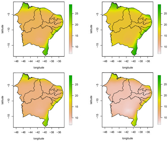
Figure 6.
Map for the 5% quantile of the minimum humidity of the air in the stations of the northeast of Brazil. (Top): January (left) and April (right). (Bottom): July (left) and October (right).
5. Concluding Remarks
This work presented a new approach for the GEV distribution for maxima, considering a reparameterization in terms of the mean and standard deviation. Considering this approach, we were able to interpret how covariates directly affect the mean and dispersion of the data. In the application proposed in this work, we were able to measure how much variables such as latitude, altitude, distance from the sea, and month of the year affect the average and dispersion of the monthly minimum humidity. With these results, we can point out which places in the northeast region of Brazil have the most critical levels of low humidity, and in which months of the year these levels occur.
This parameterization, as well as the usual GEV distribution, also allows the calculation of extreme quantiles, making it possible to obtain these estimates for each location and each month of the year. When estimating for each location, it was possible, through the interpolation method, to map the mean, dispersion, and high quantiles for the entire studied region. These results have important implications for society, as they offer authorities accurate information about which areas and months of the year are most affected by low humidity, allowing for targeted measures to protect public health. Moreover, the agricultural sector can leverage this knowledge to make precise decisions regarding the most suitable crops for each region and time of year based on local humidity patterns.
Thus, this work can be extended for a spatio-temporal modeling approach, in a scenario where these variables may reach more critical levels in the coming decades. The study also can be extended to include other environmental and socio-economic covariates, including precipitation, temperature, and local governmental environmental policies.
Author Contributions
Conceptualization, F.F.d.N.; Methodology, L.R.d.S.C., F.F.d.N. and M.B.; Software, L.R.d.S.C. and F.F.d.N.; Data curation, F.F.d.N. and L.R.d.S.C.; Writing—original draft, L.R.d.S.C.; Writing—review & editing, F.F.d.N. and M.B.; Supervision, F.F.d.N. and M.B. All authors have read and agreed to the published version of the manuscript.
Funding
This research received no external funding.
Data Availability Statement
The original contributions presented in this study are included in the article. Further inquiries can be directed to the corresponding author.
Conflicts of Interest
The authors declare no conflicts of interest.
References
- Parmesan, C.; Root, T.L.; Willing, M.R. Impacts of Extreme Weather and Climate on Terrestrial Biota. Bull. Am. Meteorol. Soc. 2000, 81, 443–450. [Google Scholar] [CrossRef]
- Sang, H.; Gelfand, A. Hierarchical modeling for extreme values observed over space and time. Environ. Ecol. Stat. 2009, 16, 407–426. [Google Scholar] [CrossRef]
- Jolliet, O. Hortitrans, a model for predicting and optimizing humidity and transpiration in greenhouses. J. Agric. Enginering Resour. 1994, 57, 23–37. [Google Scholar] [CrossRef]
- von Mises, R. La distribution de la plus grande de n valeurs. Am. Math. Soc. 1954, 2, 271–294. [Google Scholar]
- Jenkinson, A.F. The frequency distribution of the annual maximum (or minimum) values of meteorological events. Q. J. R. Meteorol. Soc. 1955, 81, 158–171. [Google Scholar] [CrossRef]
- Santos-Neto, M.; Cysneiros, F.; Leiva, V.; Ahmed, S. On new parametrizations of the Birnbaum-Saunders distribution. Pak. J. Stat. 2012, 28, 1–26. [Google Scholar]
- Hashimoto, E.M.; Ortega, E.M.M.; Cordeiro, G.M.; Cancho, V.G.; Silva, I. The re-parameterized inverse Gaussian regression to model length of stay of COVID-19 patients in the public health care system of Piracicaba, Brazil. J. Appl. Stat. 2022, 50, 1665–1685. [Google Scholar] [CrossRef]
- Bourguignon, M.; Gallardo, D.I. Reparameterized inverse gamma regression models with varying precision. Stat. Neerl. 2020, 74, 611–627. [Google Scholar] [CrossRef]
- Bourguignon, M.; Santos-Neto, M.; de Castro, M. A new regression model for positive random variables with skewed and long tail. METRON 2021, 79, 33–55. [Google Scholar] [CrossRef]
- Bourguignon, M.; Gallardo, D.I.; Gómez, H.J. A Note on Pareto-Type Distributions Parameterized by Its Mean and Precision Parameters. Mathematics 2022, 10, 528. [Google Scholar] [CrossRef]
- Bourguignon, M.; Gallardo, D.I. A general and unified class of gamma regression models. Chemom. Intell. Lab. Syst. 2025, 261, 105382. [Google Scholar] [CrossRef]
- Bourguignon, M.; Gallardo, D.I. A general and unified parameterization of the beta distribution: A flexible and robust beta regression model. Stat. Neerl. 2025, 79, e70007. [Google Scholar] [CrossRef]
- Cepeda-Cuervo, E. Beta Regression Models: Joint Mean and Variance Modeling. J. Stat. Theory Pract. 2015, 9, 134–145. [Google Scholar] [CrossRef]
- Kokonendji, C.; de Medeiros, R.; Bourguignon, M. Mean and Variance for Count Regression Models Based on Reparameterized Distributions. Sankhya B 2024, 86, 280–310. [Google Scholar] [CrossRef]
- Bourguignon, M.; Nascimento, F.F. Regression models for exceedance data: A new approach. Stat. Methods Appl. 2021, 30, 157–173. [Google Scholar] [CrossRef]
- Nascimento, F.F.; Bourguignon, M. Bayesian time-varying quantile regression to extremes. Environmetrics 2020, 31, e2596. [Google Scholar] [CrossRef]
- Gamerman, D.; Lopes, H.F. Markov Chain Monte Carlo: Stochastic Simulation for Bayesian Inference, 2nd ed.; Chapman and Hall/CRC: Baton Rouge, LA, USA, 2006. [Google Scholar]
- Nascimento, F.F.; Gamerman, D.; Lopes, H.F. Regression models for exceedance data via the full likelihood. Environ. Ecol. Stat. 2011, 18, 495–512. [Google Scholar] [CrossRef]
- Lima, S.; Nascimento, F.F.; Ferraz, V.R.S. Regression models for time-varying extremes. J. Stat. Comput. Simul. 2018, 88, 235–249. [Google Scholar] [CrossRef]
- R Core Team. R: A Language and Environment for Statistical Computing; R Foundation for Statistical Computing: Vienna, Austria, 2023. [Google Scholar]
- Diggle, P.; Ribeiro, P.J. Model-Based Geostatistics; Springer Series in Statistics; Springer: New York, NY, USA, 2007. [Google Scholar]
Disclaimer/Publisher’s Note: The statements, opinions and data contained in all publications are solely those of the individual author(s) and contributor(s) and not of MDPI and/or the editor(s). MDPI and/or the editor(s) disclaim responsibility for any injury to people or property resulting from any ideas, methods, instructions or products referred to in the content. |
© 2025 by the authors. Licensee MDPI, Basel, Switzerland. This article is an open access article distributed under the terms and conditions of the Creative Commons Attribution (CC BY) license (https://creativecommons.org/licenses/by/4.0/).