Abstract
Ensuring the smooth production and distribution of agricultural products is a crucial pathway to achieving a balance between supply and demand. However, the information within the agricultural product supply chain is characterized by its dynamic and asymmetric nature, compounded by frequent outbreaks of infectious diseases that lead to supply interruptions and allocation difficulties. These factors collectively undermine the operational efficiency and resilience of the agricultural product supply chain. This study develops an integrated allocation-location optimization model for emergency agricultural product supply chains based on a rolling horizon approach. The model accounts for both supply shortage and sufficient scenarios, with objectives to maximize the comprehensive material satisfaction rate, minimize the activation cost of distribution centers, and minimize allocation time. The proposed model is solved using the Benders decomposition algorithm. Finally, a case study based on the Shanghai pandemic outbreak is conducted for numerical simulation. The results demonstrate the effectiveness of the model: the comprehensive material satisfaction rate increases progressively over the rolling periods, rising from approximately 84% in period 1 to 100% by period 3. Furthermore, fairness analysis confirms that the model also effectively ensures equitable distribution of supplies.
Keywords:
agri-product logistics; emergency management; material allocation and distribution; facility location; rolling horizon optimization MSC:
90B06
1. Introduction
As essential commodities for daily life, the stable supply of agricultural products is crucial to national welfare and social stability [1]. In recent years, frequent outbreaks of sudden infectious diseases have severely challenged the resilience of urban agricultural supply chains [2,3]. Shanghai, for example, is a megacity with extreme population density and relies on external sources for over 70% of its agricultural products [4]. Such high external dependency creates significant regional disruption risks during disasters. During spring 2022, agricultural shortages in parts of Shanghai revealed systemic vulnerabilities: blocked production–marketing networks reduced logistics efficiency, cross-regional transportation capacity was constrained, and intense demand fluctuations coupled with inadequate data-sharing mechanisms exacerbated structural imbalances in resource allocation. Against this backdrop, establishing government-led emergency supply systems capable of precise multi-category allocation and efficient distribution has become imperative for urban crisis management.
Current emergency supply chain management faces a dual deepening challenge. First, due to the uncertainty in consumer demand and the variability of preferences for multi-category agricultural products, the sales volume in demand markets is highly dynamic. Production and sales information drives allocation decisions and serves as a prerequisite for efficiently implementing the supply and allocation of multi-category agricultural products. Second, emergency supply assurance of agricultural products involves multi-level nodes from “origins→distribution centers→demand markets,” requiring integrated solutions for the coupling of facility location, route optimization, and resource allocation. It is particularly important to note that agricultural products are characterized by high time-sensitivity and category heterogeneity, demanding that allocation simultaneously meets triple constraints: fairness, cost, and response time. This places higher requirements on the precision and sophistication of decision-making models.
To address these challenges, this study proposes a rolling-horizon-driven optimization framework for the location and allocation of multi-category agricultural products in emergency supply chains. The main contributions are as follows:
- By incorporating a rolling-horizon mechanism to update information on agricultural output, market demand, and previous allocation results, a model is constructed that accounts for both shortage and sufficient scenarios, enabling dynamic adjustment of distribution center activation strategies and allocation plans.
- Based on a three-tier supply network architecture, an integrated location-allocation optimization model is developed. Large-scale (Level A) distribution centers consolidate cross-regional supplies, while last-mile (Level B) centers precisely connect with community demand, thereby shortening supply chain response time.
- A balance between fairness and efficiency is achieved by pursuing the triple objectives of maximizing the comprehensive fulfillment rate, minimizing allocation time, and reducing activation cost. A minimum material fulfillment rate constraint is introduced to eliminate long-term shortage risks and avoid resource mismatch and wastage.
The remainder of the paper is structured as follows. Section 2 reviews material allocation and facility location literature; Section 3 formalizes the problem framework with dynamic data, tri-echelon network, and rolling-horizon mechanisms; Section 4 develops the integrated location-allocation MIP model; Section 5 implements the Benders decomposition solution algorithm; Section 6 validates the model through Shanghai case studies and sensitivity analyses; Section 7 concludes with theoretical and managerial implications. The research approach of this paper is shown in Figure 1. This research provides actionable insights for developing integrated routine-emergency agricultural supply systems, ensuring equitable distribution during shortages while preventing waste during abundance.
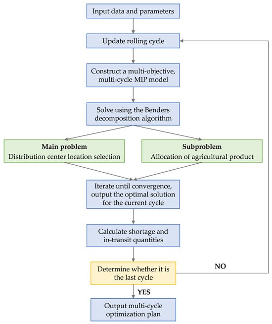
Figure 1.
Research approach diagram.
2. Literature Review
Research on emergency supply chains focuses on optimizing resource allocation in disaster scenarios, covering two core areas: materiel allocation and facility location. This section systematically reviews research progress on static and dynamic allocation models, as well as single-level and multi-level facility location problems, highlighting the limitations of existing studies and the innovative contributions of this research.
2.1. Materiel Allocation
Materiel allocation research aims to achieve precise matching of supply and demand after disasters through modeling and algorithms, minimizing socio-economic losses and ensuring basic livelihood needs [1,2,3]. Based on assumptions about the dynamic characteristics of supply and demand, relevant research can be categorized into static allocation and dynamic allocation models, focusing on topics such as government material reserves, emergency response, and equitable distribution of resources.
In static allocation models, research typically focuses on optimization under fixed supply and demand conditions. Government physical reserves are the primary means of ensuring basic materiel supply [5,6], but they face significant limitations in flexibility and cost-effectiveness. To address this, scholars have extensively explored government–enterprise collaboration models to enhance supply capacity. For example, Xie et al. [7] introduced corporate social responsibility (CSR) and government subsidy mechanisms; Arabi et al. [8], with Tian and Mei [9], developed supply chain planning models for scenarios with disruption risks and regional emergency systems, respectively; and He et al. [10] utilized 3D printing technology to optimize production and scheduling efficiency during public health emergencies. However, such studies often overlook the time-varying nature of supply and demand states, making it difficult to effectively respond to uncertainties during disaster evolution.
Dynamic allocation models, on the other hand, focus on integrating dynamic real-time information to enhance decision-making responsiveness [11]. Hao et al. [12] established a procurement optimization model based on multi-dimensional risk assessment; Ren et al. [13] developed a logistics allocation model under uncertain conditions, reflecting the trend toward data-driven decision-making. Technological applications have further advanced this field: Qi et al. [14] proposed an IT-supported rapid-response manufacturing model; Li et al. [15] used multi-agent simulation to reveal the impact of cooperation levels on emergency response. In recent years, rolling horizon planning (RHP) has gained widespread attention as an effective framework for handling dynamic uncertainties. Fattahi and Govindan [16] developed a data-driven rolling horizon approach for dynamic supply chain network design, effectively addressing disruptions and demand uncertainties; Herding and Mönch [17] applied it to short-term supply–demand matching in semiconductor supply chains, significantly improving delivery stability and resource utilization efficiency. In the field of perishable goods allocation, Lejarza et al. [18] combined rolling optimization with product quality estimation to achieve online management and optimization of perishable inventory; Sheikholeslami and Zarrinpoor [19] designed a Lagrangian relaxation-based logistics model for perishable emergency goods. Additionally, Hosseini-Motlagh et al. [20] used rolling planning to dynamically optimize blood collection strategies; Cheng et al. [21] established a robust rolling model for steel raw material procurement; Ghasemi et al. [22] extended the rolling horizon method to multi-level systems in the pulp and paper industry; and Fattahi et al. [23] further applied it to medical resource planning and real-time decision-making during pandemics.
It is noteworthy that fair allocation and shortage response are core challenges in emergency materiel allocation. Existing research primarily employs multi-objective optimization methods. For instance, Zhou et al. [24] aimed to minimize road risks and materiel shortfalls; Cao et al. [25] incorporated victim perception satisfaction into a mixed-integer model; Ruan et al. [26] used interval number preferences to address fair allocation under heterogeneous data. For dynamic shortage scenarios, Liu et al. [27] proposed a fair allocation framework under time-varying supply and demand constraints, while Lee [28] designed a resilient capacity allocation strategy under supply failure risks. However, most existing models are based on static supply assumptions [29,30], failing to fully capture the dynamic evolution of supply and demand in disaster environments, and there is a particular lack of studies that simultaneously consider both shortage and sufficient scenarios.
In summary, while existing research on materiel allocation is rich in model construction and algorithm design, studies on the end-to-end allocation and distribution of agricultural products remain insufficient. Moreover, most research assumes a static materiel supply. In reality, the dynamic and uncertain nature of supply and demand information during emergencies leads to temporary shortages in the early stages, with supply and demand gradually balancing as resources are mobilized. Therefore, developing a dynamic allocation model that ensures fairness during shortages and avoids waste during surpluses holds significant theoretical innovation and practical application value.
2.2. Facility Location
Facility location studies have evolved from single-level independent site selection to multi-level system-level collaborative optimization. In recent years, there has been increased focus on joint decision-making with material allocation to better address complex constraints and uncertain environments in emergency logistics.
Single-level facility location has developed a relatively mature research framework, primarily focusing on the spatial layout optimization of nodes such as storage depots and distribution centers [31]. Based on the duration of facility operation, this can be categorized into temporary [32] and permanent facility location [33]. To address uncertainties, methods such as dynamic location [34], robust optimization [35], and stochastic programming [36] have been developed. Giusti et al. [37] constructed a multi-service transit hub location model considering demand volatility and customer flexibility; Li et al. [38], with Eydi and Shirinbayan [39] employed two-stage robust optimization and a hierarchical indicator method, respectively, to tackle demand uncertainty. For further detailed discussion and future research directions on single-level facility location problems, please refer to the review articles by Boonmee et al. [40] and Wang et al. [41]. While these studies provide a methodological foundation for emergency facility location, most are limited to a single level and fail to fully capture the multi-level nested characteristics of emergency networks.
Building on this, academia has gradually shifted focus to the joint optimization of facility location and materiel allocation, centering on the layout and resource coordination of facilities such as emergency shelters, logistics hubs, and medical aid stations. Shaw et al. [42] optimized a distribution center location from a humanitarian logistics perspective; Liu et al. [43] integrated the location of temporary medical sites with limited resource allocation; Geng et al. [44] introduced a pain-perception cost to optimize government–enterprise joint emergency response; Khayal et al. [45] designed a network flow model with dynamically adjustable resources; Vahdani et al. [46] further integrated facility location, district partitioning, and vehicle routing problems, reflecting a research trend towards multi-link coordination; Yoruk et al. [47] addressed humanitarian relief logistics by jointly optimizing the location of disaster stations and the replenishment of perishable relief supplies. Although these studies have made significant progress in model complexity and practicality, most still concentrate on single-level facility networks or, while involving multi-level structures, lack in-depth analysis of inter-level capacity constraints, flow coordination, and dynamic adjustment mechanisms.
In summary, facility location research has progressed from single-level independent location problems to multi-level system joint optimization, gradually incorporating uncertainty factors. Although the integrated optimization of facility location and materiel allocation has achieved some progress, further coupling with other supply chain segments is necessary to better respond to the complexity of disaster scenarios and the diversity of demands. Moreover, existing research predominantly focuses on the integrated optimization of single-level facility location, often aiming for efficiency maximization or cost minimization. Studies on the integrated optimization of multi-level facility location and materiel allocation remain limited. Therefore, determining how to balance the advantages and disadvantages of locating multi-level transit facilities under multiple constraints such as cost, flow, distance, and time constitutes a scientific problem worthy of in-depth investigation.
3. Model Description and Assumptions
3.1. Model Description
As essential material foundations for residents’ livelihoods, local governments must ensure stable production and guaranteed supply of agricultural products. However, urban agricultural supply systems continue to reveal vulnerabilities when confronting emergencies such as infectious disease outbreaks:
- (1)
- There is an inefficient production–marketing linkage networks. Comparative analysis of supply structures before and after outbreaks demonstrates that stringent controls imposed at each logistics node—though necessary for safety—diminish efficiency in supply provision, transshipment, and transportation.
- (2)
- The demand and supply data of agricultural products are in dynamic change, and the demand for multi-category agricultural products often cannot be satisfied at one time, so the government-led agricultural products production and marketing docking needs to be based on the dynamically updated production and marketing data to make multiple allocation decisions.
- (3)
- There is insufficient sharing of data related to the production and marketing of agricultural products between the government and society. The circulation of agricultural products involves producers, markets, distributors, logistics enterprises and other subjects, and it is difficult to keep abreast of the demand and supply situation in various regions and markets, which leads to uneven distribution of materials and creates great difficulties in the unified management and allocation of agricultural products and materials.
Under special circumstances, the conventional market circulation system can no longer meet the supply demand of agricultural products in the whole city, and there is an urgent need for an efficient and stable supply system, one which coordinates the resources of material, human and financial resources; builds a transportation and transit network of two-tier distribution centers in the city, one which buttresses multiple agricultural product origins for direct picking and allocates them to multiple markets in demand; and is responsible for distribution and transportation of agricultural products, which accurately matches the two ends of the demand and supply and guarantees the fair and reasonable distribution of agricultural products under the situation of shortage of supply. It can accurately match the supply and demand and guarantee the fairness and reasonableness of the distribution of agricultural products in case of supply shortage.
To address these challenges, this study considers two scenarios, i.e., the supply of agricultural products is in short supply in the early stage and the supply of agricultural products is sufficient in the late stage (the sufficient-supply scenario denotes balanced or mildly excess capacity, distinct from structural surplus involving significant waste penalties), and builds an agricultural supply and distribution system. This system not only plans the quantity of materials to be distributed to the demand market, but also decides on the location of the alternative distribution centers and the demand market it serves, a “supply point-transit point-demand point” three-layer supply chain network (as shown in Figure 2). This network contains important nodes, as follows:
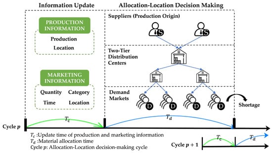
Figure 2.
The process of allocating agricultural products based on rolling updates of production and marketing information.
- (1)
- Supply points, or agricultural production origins: Generally speaking, each production base will produce one to more categories of agricultural products, such as vegetable planting bases, pig farms and so on;
- (2)
- Transit point: The agricultural product collection and distribution center, as a transshipment point for the government’s emergency allocation, has two main functions, namely, collecting and distributing goods, and is responsible for the centralized storage, sorting, disinfection and centralized distribution of multi-category agricultural products and materials, and other functions;
- (3)
- Demand points, or the demand market for agricultural products, medium- and large-scale supermarkets, wholesale markets, farmers’ markets, etc.: These are the locations at which urban residents buy agricultural products on-line and close to their homes, and which are the main sales channels for agricultural products, with the wholesale market being the main focus, and the circulation and delivery of fresh agricultural products to the end communities continuing.
Considering that the production and marketing data will change dynamically over time, which further affects the effectiveness of the agricultural supply and distribution allocation work, this study divides the whole process into multiple allocation time cycles when planning for the distribution of supplies, and each allocation cycle consists of the time of ordering agricultural products in the demand market (production and marketing data collection) and the time of scheduling the agricultural products supplies. Since this research model does not consider the specific delivery process of materials, the redeployment cycle of this study is the average interval of the order consolidation and processing time in the demand market. Joint decision-making on redeployment volume and consolidation and distribution center location is carried out through rolling horizon.
When cycle of allocation decision-making begins, it first dynamically updates its production and marketing data, and, under the condition of guaranteeing the minimum material satisfaction rate of each demand market, it only needs to carry out allocation planning for multi-category agricultural products in the current cycle based on the production and marketing data summarized in the current cycle and the results of the allocation decision-making of the previous cycle (shortages of agricultural products ). This is undertaken so as to formulate the optimal emergency agricultural products supply and distribution allocation plan in the current cycle, and to guarantee the fairness of distribution and the material satisfaction rate of the demand markets as well as the fairness of the distribution of the allocation quantity and the material satisfaction rate of the demand market in each cycle. Then, in all cycle times, due to the limited material dispatching capacity of the centralized distribution center and the fact that the allocated quantity will be transferred to the demand market in the centralized distribution center, it will search for the optimal two-tier centralized distribution center location plan with the goal of minimizing the time and cost of allocation under the constraints of throughput to construct the supply guarantee network. The model will set up a large-scale centralized distribution center in charge of the centralization, integration, and management of the material of multiple categories of agricultural products, and then transport designated agricultural products to the end of the centralized distribution center in batches. The large-scale distribution center is responsible for the concentration, integration and management of multi-category agricultural products, and then the designated agricultural products are transported in bulk to the terminal distribution center, which is responsible for the centralized distribution of agricultural products to the demand market, thus guaranteeing the stable supply of a variety of materials in the context of regular or emergency events.
3.2. Model Symbol Description
To facilitate understanding of the meaning of relevant mathematical symbols in the model, this section provides a unified definition of the mathematical symbols used for sets, variables, and parameters in the model for reference, as shown in the following (Table 1):

Table 1.
Summary of key notation involved in the model.
3.3. Model Assumptions
Since this study mainly focuses on optimizing emergency supply chain decisions for agricultural products in the context of public emergencies (such as infectious disease outbreaks), the model constructed is based on the following assumptions:
Assumption 1:
The location of the demand market for agricultural products, the distribution centers and the production and supply origins, as well as the distance between any two points, are known, and each agricultural production origin offers one category of agricultural products.
Assumption 2:
Production and sales volume will fluctuate over time, this study counts the production and sales data generated in each cycle, the sales data of agricultural products in each demand market can be shared in a timely manner, and the sales volume of each category of agricultural products in each demand market in each cycle, the production of each category of agricultural products, as well as the throughput of collection and distribution centers are known.
Assumption 3:
This study does not take into account the effects of road damage and changes in weather, the problems that arise in the management of emergency dispatch, the round-trip utilization of means of transport and the depletion of the transport process.
Assumption 4:
Considering the cost or resource constraints, the distribution centers have limited material handling capacity, and there is a cost associated with opening alternative distribution centers. Emergency agricultural products need to arrive at the distribution center from the origin before being transported to the market in the place of sale, and there is a many-to-many correspondence between the distribution center and the demand market.
Assumption 5:
The dynamic characteristics of the rolling horizon are targeted at the transfer volume of multi-category agricultural products and enabled distribution centers, and can only be enabled to dock with other points. The model is not involved in the specific transport process of the material, but only the transfer volume and distribution center location planning decisions.
Assumption 6:
Local governments make decisions on the allocation of multi-category agricultural supplies based on production and marketing data updated each cycle and shortages from the previous cycle, with cycle lengths greater than the supply dispatch time.
4. Model Formulation
For each allocation cycle , three factors are considered—the comprehensive satisfaction rate of agricultural products, allocation time, and the cost of activating distribution centers—to construct a mixed-integer programming model for joint decision-making on allocation and location selection.
4.1. Comprehensive Satisfaction Rate of Agricultural Products During the Cycle
The satisfaction rate of agricultural products in a certain area during a specific time cycle is defined as the ratio of the received quantity to the demand quantity. Regardless of whether there is a shortage or surplus of materials, this model aims to maximize the sum of the comprehensive satisfaction rates of all product categories in all cycles, namely the ratio of allocation to the sum of sales volume and shortage in the previous cycle. This is achieved by ensuring that agricultural products are delivered to demand markets as much as possible and that allocation is fair. The objective function for the satisfaction rate of multiple categories of agricultural products is shown in Equation (1).
4.2. Allocation Time During the Cycle
Considering the urgency and continuity of material allocation, multiple categories of agricultural products are mainly shipped from production origins to demand markets. Therefore, the emergency allocation time is represented by the total scheduling time from production origins to demand markets, as shown in Equation (2).
means the sum of scheduling time from the origin of each category to the large-scale distribution center. means the sum of scheduling time from the large-scale distribution center to the terminal distribution center. means the sum of scheduling time from the terminal distribution center to various demand markets.
4.3. Cost of Activating Distribution Centers During the Cycle
When emergency supply facilities are insufficient, distribution centers are set up to connect multiple production origins, and terminal distribution centers connect to multiple demand markets, establishing a two-tier transfer and allocation transportation network. The activation of distribution centers incurs certain costs, and this study temporarily considers only the transfer costs, as shown in Equation (3).
Additionally, based on the assumptions, parameter settings, and problem analysis of this study, consider constraints such as the relationship between supply and demand of emergency agricultural products, the minimum demand satisfaction rate, and the throughput of the distribution center while making decisions. The model constraints are defined in Equations (4)–(16).
Equation (4) states that the allocation quantity of any agricultural product by the government to the demand market cannot exceed the actual supply of that product. Equation (5) establishes a minimum supply satisfaction rate constraint to ensure that the total agricultural products allocated to each demand market after allocation does not fall below a specified proportion of the sum of its current sales volume and the previous cycle’s shortage volume. This constraint enables decision-makers to prioritize meeting the basic needs of severely deficient regions under resource constraints, thereby preventing deterioration in fairness. Simultaneously, it provides a clear basis for evaluating the fairness of allocation plans, contributing to enhanced rationality in material allocation strategies and greater social stability. Equation (6) indicates that the allocation quantity to the demand market cannot exceed the sum of sales and the shortage from the previous cycle. Equations (7) and (8) ensure that the total quantity of agricultural products received and delivered at any distribution center does not exceed its processing capacity. Additionally, transportation of agricultural products is permitted only when the distribution centers are operational, ensuring that material flows occur exclusively under activated conditions. Equation (9) defines the relationship between variables and , stipulating that scheduling services to demand markets can be initiated only if the corresponding terminal distribution centers are operational. Equations (10) and (11) define the relationship between variables , and , specifying that only when both the superior and inferior distribution centers are operational can a large-scale distribution center provide agricultural product transportation services to a terminal distribution center. Equation (12) indicates that each demand market can be served by only one terminal distribution center. Equation (13) defines that a terminal distribution center can only be connected to one large-scale distribution center. Equation (14) states that when a distribution center is activated, it will be connected to the production origin. Equations (15) and (16) define the types of decision variables. Specifically, the activation status of the distribution center is a variable, and the quantity of agricultural product allocation for each demand market is a non—negative real number.
Following the allocation decision-making process, the shortage quantity for each agricultural product category at every demand market is calculated before the next cycle commences. This serves as critical input for subsequent allocation planning, as formalized by the state transition Equation (17). The shortage metric quantifies unmet demand within the emergency supply chain. To streamline modeling, we assume all demand is fulfilled when actual sales fall below allocated quantities , thus setting in such cases.
The production–marketing data-driven allocation model incorporates three objective functions, the first of which is to maximize the comprehensive satisfaction rate, while the other two are minimization problems. To unify the solution method for multi-objective models, the original objective function is converted into a minimization problem, as shown in Equation (18):
Given the differing dimensions and polarity among the three objective functions, this study employs the normalization method to transform them into standardized dimensionless forms, enabling the construction of a unified weighted objective function. As a data preprocessing technique, normalization eliminates dimensional disparities in multi-objective optimization by linearly mapping original objective values to a uniform interval (typically ) through extremum anchoring. This linearization preserves structural boundaries without introducing relaxation, thus avoiding structural errors [48]. After standardization, the numerical values of each objective fluctuate within a unified range, and their variation magnitude and relative importance can be flexibly adjusted through weight coefficients. If decision-makers prioritize a specific objective (such as shortening allocation time), they need only assign it a higher weight. A minor improvement in that objective will then significantly impact the overall objective value, thereby guiding the selection of solutions. This mechanism enables the model to adapt to different emergency scenarios and decision-making preferences. During the initial disaster phase, emphasis can be placed on allocation efficiency and fairness, while the focus may shift to cost control during the recovery phase. Furthermore, since all objectives are expressed in the same numerical scale, weight allocation is no longer influenced by original units of measurement, enhancing the transparency and interpretability of the multi-objective optimization process.
The upper and lower bounds of the objective function can be obtained by calculating the extremal values of the relevant constraints. For instance, when considering only the satisfaction rate of agricultural products, the lower bound is derived from the boundary of constraint (5), representing the minimum overall satisfaction rate. The upper bound s calculated based on Equations (4) and (6), reflecting the maximum comprehensive satisfaction rate across all demand markets over all cycles. (allocation time) bounds based on shortest/longest path times between all node pairs. (activation cost) bounds from minimal/maximal distribution center activation costs. In addition, assuming are the weighting coefficients for the three objective functions, with , the composite objective function is constructed as shown in Equation (19).
5. Solving Method
The multi-cycle allocation-distribution problem studied in this paper constitutes a combinatorial optimization challenge involving joint decisions on multi-category agricultural product allocation and distribution center location across multiple supply points, transit nodes, and demand points. Formulated as a mixed 0–1 integer programming model, it faces computational complexities including large-scale solving, nonlinearity, and multi-constraint issues. Benders decomposition algorithm—with its high solving efficiency and strong convergence properties—proves particularly suitable for accurately solving medium-to-large-scale mixed-integer linear programming problems. Furthermore, the rolling-cycle characteristic enables iterative application of Benders decomposition to obtain optimal allocation-distribution solutions within each cycle, thereby achieving global optimality across the entire time horizon. For instance, the algorithm first derives optimal allocation and facility scheduling solutions using Cycle 1’s production–marketing data, then calculates resulting shortages and in-transit inventory at distribution centers. These outputs become inputs for the optimization of Cycle 2, effectively transforming the multi-cycle model into a sequential single-cycle optimization framework. The subsequent section elaborates on the Benders decomposition procedure for this model.
5.1. Constraint Linearization
To simplify the model complexity into a rolling optimization for a single cycle, non-linear constraints in the supply and allocation model are linearized by introducing auxiliary variables, as shown in Table 2.
Table 2.
Summary of auxiliary variables for constraint linearization.
After transforming the simplified model complexity into a rolling optimization for a single cycle, considering that constraints (7) and (8) in the supply and allocation model are nonlinear, define . represents an upper bound on the allocation quantity, set as a sufficiently large constant. Introducing auxiliary variables, if , , then ; if , then . Consequently, the auxiliary constraint is added as shown in Equation (20).
Define only when , . The auxiliary constraint is thus expressed by the following Equation (21).
Consequently, it is transformed into a mixed-integer linear programming problem.
5.2. Subproblems and Main Problem
Based on the different variable types, the original problem is decomposed into a main problem and subproblems. The main problem is responsible for solving the integer variables, while the subproblems handle the continuous variables through iterative solution. For the multi-cycle agricultural product supply and allocation model developed in this study, only is a continuous variable; all others are binary variables. Therefore, the allocation decision is divided into subproblems, with the selection of two-tier distribution centers as the main problem, as detailed below.
5.2.1. Subproblems and Dual Problems
The linear programming subproblems resulting from model decomposition are expressed in Equations (22)–(35), where ,, represent pre-determined facility location plans, which can be regarded as constants, and denotes the shortage amount caused by the allocation plan in the previous cycle.
Based on the sub-problems, multiple dual variables are constructed, each corresponding to the constraints expressed in Equations (23)–(34). These variables take on any real values greater than or equal to zero. The objective function of the dual problem is as shown in Equation (36).
5.2.2. The Main Problem and the Relaxed Main Problem
The main problem is a 0–1 programming problem, excluding continuous variables and their constraints, as shown in Equations (37)–(46). When there is a shortage in periodic supply, additional constraints—Equations (45) and (46)—are introduced to prevent certain facility location and scheduling schemes from resulting in transfer volumes exceeding the processing capacity of the distribution centers, which would render the subproblem infeasible. When the periodic supply is abundant, to ensure that the satisfaction rate of all demand markets reaches 100%, and to avoid reducing transfer volumes solely to balance costs and timeliness, the adjustments to Equations (45) and (46) do not need to multiply the minimum satisfaction rate . Instead, facility location schemes are determined based on sales volume and inventory levels.
Solving the dual model of the subproblem via the simplex method, when the subproblem is feasible and bounded, the optimal values of the dual variables can be used to construct an optimal cutting plane, which is then incorporated into the master problem model. Let denote the optimal values of all dual variables of the subproblem; here, the added cutting plane is represented as in Equation (48). When the subproblem is unbounded, signifies the extreme directions of all dual variables; in this case, the feasible cutting plane is given by Equation (49). Furthermore, an auxiliary continuous variable is introduced to measure the current optimal and feasible cuts, serving as an upper bound for the portion of the original problem’s objective function involving the continuous variables , specifically . When an optimal solution exists, , a relaxed master problem is constructed, as shown in Equations (38)–(49).
5.3. Benders Algorithmic Solution Steps
Due to dynamic input data variations across cycles—including supply quantities, demand volumes, and inventory states—the subproblem structure and feasible region may undergo significant changes. Inheriting cuts from prior periods risks over-restricting the current feasible region and potentially causing invalid cuts that erroneously exclude feasible solutions, thereby compromising solving stability. To mitigate this, our approach implements a periodic reinitialization mechanism, whereby the Benders decomposition algorithm is reset and executed from scratch within each rolling cycle, deliberately discarding accumulated cuts from previous periods. The flowchart for the Benders decomposition solution algorithm is shown in Figure 3.
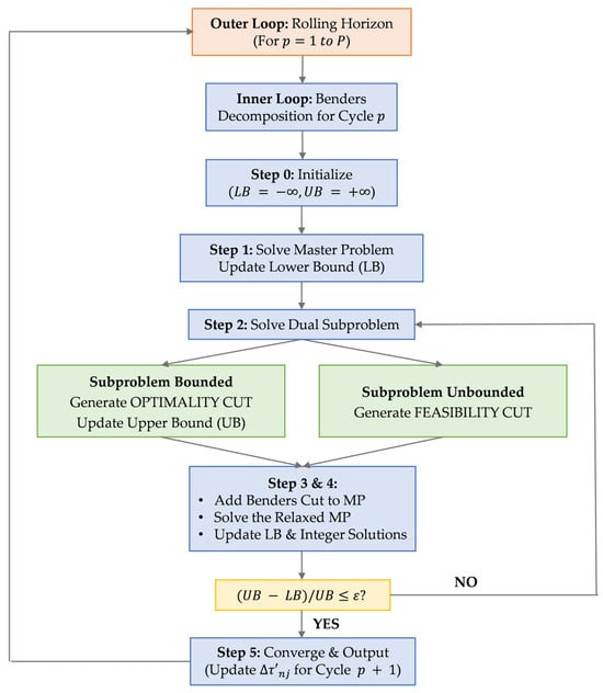
Figure 3.
Flowchart of the Benders decomposition solution algorithm.
First, initialize the initial shortage amount . For each cycle , update the production and sales data along with the previous cycle’s shortage parameters, then execute the Benders decomposition algorithm to solve for the optimal allocation and facility location plan in the current cycle. Repeat this process iteratively until the entire planning horizon achieves optimality.
(1) Initialization involves setting the convergence tolerance , the global upper bound , and the global lower bound . Input the parameters for cycle , etc.) along with the upper and lower bounds of the objective functions, and ). These bounds can be obtained by adjusting the target coefficients and running the algorithm to find the extremal values under the relevant constraints.
(2) Solve the main problem defined by Equations (37)–(46), obtaining the objective function value and the integer variables , , and . Simultaneously, update the global lower bound .
(3) Based on the current values of , , and , solve the dual subproblem to obtain the dual variables.
- If an optimal solution exists, determine the subproblem’s objective value and the optimal dual variables . Update the upper bound as . Construct the optimal Benders cut by substituting into Equation (48). In this research, Gurobi is invoked via Constr.Pi in PyCharm to directly obtain the dual variables of the subproblem’s optimal solution, which are then added to the relaxed master problem.
- If no feasible solution exists, determine the extreme direction of the dual subproblem. Using Constr.FarkasDual, Gurobi is called to obtain the dual variables associated with the infeasibility, constructing a feasible cut by substituting into Equation (49) and adding it to the relaxed master problem. This Benders cut excludes the current , and that lead to infeasibility in subsequent iterations.
(4) Solve the updated relaxed main problem to obtain the optimal solution , . Update the lower bound as and set , , and .
(5) Check whether . If the stopping criterion is met, terminate the iteration, output the results, update the cycle shortage amount , and return to step (1). Otherwise, return to step (3).
The pseudocode for the Benders decomposition algorithm is summarized in Algorithm 1.
| Algorithm 1. Pseudocode for the Benders decomposition solution algorithm |
| Benders Algorithmic Solution Steps |
| For to do |
| Step 0. Initialization: |
| Input parameters (); Input , and set |
| Step 1. Solve the Master problem in equation set (37)–(46): |
| Get , , update ; |
| while do |
| Step 2. Solve the dual subproblem based on , : |
| If unbound then: |
| Get extreme ray (); Add to Master problem the Benders feasibility cut (constraint (49)); |
| else Get extreme point (); Add to Master problem the Benders optimality cut (constraint (48)); Update ; |
| End if |
| Step 3. Solve the Relaxation Master problem: |
| Get ; |
| Step 4. Update , ; |
| End while |
| Step 5. Output the and update ; |
| End for |
6. Case Analysis
All numerical simulations in this section were performed using PyCharm Community Edition 2022.3.1 and Gurobi 10.0.0. The simulations were executed and compiled on an Intel® Core™ i5-8265U CPU @ 1.60 GHz (four cores) system with 8 GB RAM.
6.1. Case Setup
The numerical case study examines emergency supply assurance for Shanghai’s agricultural supply chain during the Spring 2022 infectious disease outbreak. To verify the feasibility of the model and the effectiveness of the algorithm, agricultural products with large daily consumption by residents—green vegetables and pork—are selected. However, due to the perishability and short edible period of these two agricultural products, the vegetable planting base in Danyang, Jiangsu Province, and the pig farm in Dongtai (), which are close to Shanghai and have large yields, are chosen as the external continuous supply points for the two categories of agricultural products, respectively, to ensure the normal operation of part of Shanghai’s agricultural product markets. Then, alternative large distribution centers () in suburban areas are selected as primary distribution points, and terminal distribution centers () are selected as secondary distribution points. Some farmers’ markets or supermarkets () in Shanghai are selected as demand points for multi-category agricultural products, thus constructing an agricultural product production–marketing docking supply network composed of two agricultural product categories, nine alternative distribution centers, and sixteen agricultural product demand markets. Due to significant distance disparities between production origins and distribution centers—which operate at different geographical scales—we extracted spatial distribution data exclusively for distribution centers and demand nodes using Baidu Maps, as shown in Figure 4.
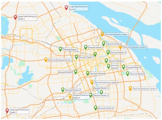
Figure 4.
Geographic distribution of distribution centers and demand markets.
The geographical distribution of all nodes—including production origins—was converted into Cartesian coordinates (unit: kilometers). Given that production origins are located significantly farther from distribution centers than the distances between distribution centers and demand markets, the coordinate points are presented in two separate diagrams for visual clarity: Figure 5a displays the spatial distribution of alternative distribution centers and agricultural demand markets . Figure 5b illustrates the spatial relationship between production origins and primary distribution centers.
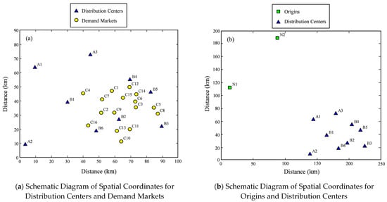
Figure 5.
Spatial coordinate diagram of origin, distribution center and demand market.
Considering Shanghai’s insufficient local agricultural supply and high population density, which drives substantial daily demand for fresh produce, local governments can implement emergency short-distance transfers through direct sourcing from production origins or neighboring cities. Furthermore, given that green vegetable and pork are highly perishable with short shelf lives and exhibit rapid demand fluctuations, allocation cycles must be minimized to prevent decision deviations or material waste. Accordingly, the rolling horizon cycle in the model is set to three cycles, balancing solvability with timely data updates and plan adjustments. Each cycle spans three days, with the first day designated for agricultural product ordering. Residents place orders every other day, with order quantities treated as the current cycle’s demand market sales volume. This demand is dynamically updated across cycles, driving allocation decisions; concurrently, allocation volumes are constrained by the supply network capacity of distribution centers, determined according to actual supply and scheduling conditions. This framework ensures responsiveness to dynamically changing demand while maintaining operational feasibility.
In this study, relevant parameters and variables are reasonably assumed according to the actual situation. The production and sales related data are from the China Agricultural Product Market Monitoring System, the Shanghai Municipal Bureau of Statistics, the Shanghai agricultural product market sales information, etc. The sales statistics of each major demand market for various categories of agricultural products in each cycle are shown in Table 3.
Table 3.
Sales of agricultural products in each cycle of demand markets.
The production data for supply points is sourced from local statistics bureaus regarding annual green vegetable production and pork output, and is processed based on cycle length to simulate dynamic production fluctuations. Specifically, the annual data from 2022 is first used to calculate the baseline average production for each 3-day cycle (approximately 122 cycles) throughout the year. To simulate the scenario where production areas proactively increase capacity to alleviate supply shortages, a random disturbance following a normal distribution is added to the base values to reflect natural fluctuations, such as weather or small-scale production changes, while also setting a growth parameter that increases with each cycle. The processed production data for fresh vegetables and pork at agricultural production areas for each cycle are shown in Table 4.
Table 4.
Production of agricultural products in each cycle of the producing area.
In this case, the scheduling time between nodes is measured in hours. Given that agricultural product allocation is generally carried out based on nearby distribution with short transportation distances, it is reasonably estimated according to the distance and the average speed of vehicles.
Table 5 and Table 6 present the scheduling times from large distribution centers to production origins and terminal distribution centers, as well as the distribution times from terminal distribution centers to demand markets, respectively.
Table 5.
Scheduling time from the large distribution center to the origin and the terminal distribution center.
Table 6.
Scheduling time from terminal distribution center to demand market.
To ensure the smooth delivery of supplies to high-risk areas, emergency authorities determine alternative distribution center locations based on supply–demand dynamics and disaster impact assessments. This study adopts reasonable assumptions for relevant parameters and variables in agricultural product allocation, referencing China’s national standard—GB/T 38375-2019 [49]—published by the Logistics Standardization Technical Committee. Each distribution center has limited periodic emergency handling capacity, with throughput variations existing both within the same tier and across different tiers. Furthermore, due to economies of scale, activation costs exhibit strong positive correlation with throughput capacity. While geographical factors introduce individual cost deviations, the overall relationship remains robust, as detailed in Table 7.
Table 7.
Throughput and enablement costs for all alternative distribution center.
To ensure that each demand market can obtain a certain proportion of agricultural product allocation under material shortage and guarantee the proportional fairness and rationality of emergency material distribution, this study sets a minimum material satisfaction rate parameter in the scheduling model, requiring that the material satisfaction rate of each category in each demand market in the allocation scheme is greater than the minimum material satisfaction rate. In addition, to reflect the rationality and balance of multi-category agricultural product allocation and distribution center location, it is assumed that the three objective functions are equally important, that is, that the coefficients are equal (). The initial parameters of the model and algorithm are set as shown in Table 8.
Table 8.
Initial parameters of model and algorithm.
6.2. Results Analysis
By using the Benders decomposition algorithm, the agricultural product allocation schemes, two-tier distribution center location plans, and objective function values are solved. The location-scheduling scheme for Shanghai’s fresh agricultural products based on production and sales data not only includes the location decisions of alternative distribution centers but also plans the transportation routes from production origins to large distribution centers, terminal distribution centers, and finally to demand markets—i.e., the supply–demand service relationships among nodes in the allocation network. The allocation scheme decides the allocation quantities of the two agricultural product categories, from which the satisfaction rate of each demand market can be obtained.
The results of the two-tier distribution center site selection are shown in Table 9. Considering comprehensive factors such as costs, satisfaction rates, and allocation timeliness, activating large distribution centers , and terminal distribution centers , , , is the optimal location scheme currently. The total activation cost is = 255 (10,000 CNY); the sum of agricultural product allocation times from production origins to all demand markets is = 36 (h), among which the longest route from production origins to demand markets takes 7 h. Meanwhile, under this scheme, the sum of comprehensive material satisfaction rates for all demand markets and product categories across all cycles is = 27.844 (%), indicating that the allocation scheme can ensure relatively high satisfaction rates for all demand markets under the condition of an 80% minimum material satisfaction rate.
Table 9.
Two-tier distribution center location allocation scheme in cycle 1.
As shown in Figure 6, the supply–demand relationships among allocation network nodes are based on the principle of nearby allocation to a certain extent. The local government purchases and transports agricultural products from production origins and to large distribution centers, which are then connected to terminal distribution centers and (for ) and and , respectively, before centralized distribution to 16 demand markets. This constructs a “production origin—distribution center—demand market” production–marketing docking network to achieve the unified procurement and distribution of agricultural products.
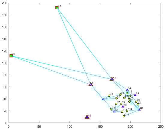
Figure 6.
Schematic diagram of the allocation network for Cycle 1.
By substituting the allocation results of Cycle 1 to calculate the agricultural product shortage amount for each market, the in-transit volume held in the distribution center in the Cycle 1 collection and distribution plan (Table 7 and Table 8), and the production and sales data of Cycle 2 into the model, the location of distribution centers plus the agricultural product allocation scheme for Cycle 2 is solved. Similarly, the location of distribution centers plus the agricultural product allocation scheme for Cycle 3 can be obtained, as shown in Table 10 and Table 11.
Table 10.
Two-tier distribution center location allocation scheme in cycle 2.
Table 11.
Two-tier distribution center location allocation scheme in cycle 3.
The total allocation time for the three cycles is 36 h each. The location schemes for Cycle 1 and Cycle 2 are the same, but the supply–demand service relationships among network nodes are different. The location scheme for Cycle 3 changes to activating distribution centers with a total activation cost of 2.66 million CNY. Meanwhile, due to sufficient supply in Cycle 3, the total allocation volume is relatively large, so its comprehensive satisfaction rate is also the highest, reaching 31.820, while the comprehensive satisfaction rate in Cycle 2 is the lowest, being 26.347.
Table 12 summarizes the allocation quantities of green vegetables and pork for each demand market in each cycle, as well as the agricultural product satisfaction rates (allocation quantity/order quantity). As shown in the “Total” column, during the early stage of emergencies, the surge in demand, constrained by insufficient supply, was the main factor restricting the maximization of the comprehensive satisfaction rate. For example, the sum of allocation quantities of green vegetables and pork in Cycle 1 was equal to the corresponding agricultural product output in Table 4. Due to the significant shortage in Cycle 1, the comprehensive material satisfaction rate in Cycle 2 was the lowest. However, as production capacity expanded in the later stage and supply gradually became sufficient, it not only needed to meet the sales volume of the current cycle but also sought to make up for the shortage of the previous cycle. Therefore, the satisfaction rate of agricultural products exceeded 100%. For instance, the agricultural products short in Cycle 2 were finally replenished in Cycle 3 with sufficient supply, which can be clearly observed as a result of the satisfaction rate of agricultural products in Cycle 3 being greater than 1. This simultaneously ensures that demand markets will not be in a state of long-term material shortage and avoids waste.
Table 12.
The volume of agricultural products allocated and the satisfaction rate per cycle of each demand market.
By integrating Table 3 and Table 12, the fulfillment rate for each agricultural product in every demand market per cycle can be determined, as shown in Table 13. Given that the comprehensive satisfaction rate is defined as the allocation quantity divided by the sum of sales and shortage from the previous cycle, it will be lower than the agricultural product satisfaction rate. From Cycle 1 to Cycle 3, the comprehensive satisfaction rate gradually increases to 100%, demonstrating that the cycle length is a reasonable choice that balances response time, model complexity, and algorithm feasibility, exhibiting comprehensive adaptability in both practical and computational terms. In addition, fresh food materials of green vegetables and pork are in a shortage state in both Cycle 1 and Cycle 2. Due to supply falling short of demand in Cycle 1, the overall material satisfaction rate remains around 85%, with only two demand markets having a comprehensive satisfaction rate of 100%, those for green vegetables and pork. Affected by the shortage quantity in Cycle 1, the number of demand markets with a comprehensive satisfaction rate of 100% further decreases to only one for each in Cycle 2. Until Cycle 3, when supply exceeds demand, the replenishment of the shortage quantity in Cycle 2 makes the agricultural product satisfaction rate of most demand markets in Cycle 3 exceed 100%, and materials in demand markets are basically satisfied. Only the satisfaction rate of pork in demand market is 85%, with a comprehensive satisfaction rate of 82%, still in shortage.
Table 13.
Statistics of satisfying rate of agricultural products per cycle in each demand market.
To evaluate the fairness of allocation decisions, this study introduces the Gini coefficient to analyze the agricultural product fulfillment rates across periods. The results indicate that fairness progressively improves throughout the allocation process, a finding with important implications for emergency resource distribution policies.
In the initial period (Cycle 1), due to limited production capacity, approximately half of the demand points only reached the minimum fulfillment rate threshold of 0.8. The Gini coefficients for vegetables and pork were 0.0545 and 0.0522, respectively, reflecting the challenge of balancing efficiency and fairness under conditions of widespread shortage. As production capacity recovered, Cycle 2 made up for some of the previous shortfalls through rolling allocation, reducing the Gini coefficients for the two types of agricultural products to 0.0322 and 0.0358, respectively. This demonstrates that the dynamic allocation mechanism can effectively enhance fairness. By Cycle 3, when the supply chain had largely recovered, the fulfillment rate for vegetables rose to above 1 across the board, and the Gini coefficient further improved to 0.0285. However, for pork, a sudden surge in demand in region C4 caused the fulfillment rate to drop to 0.85, while the other 15 demand points all exceeded 1.03. This phenomenon suggests that sudden demand spikes may affect both material fulfillment rates and allocation fairness. Therefore, in policy practice, it is essential to establish dynamic monitoring and rapid response mechanisms. Local governments need to promptly adjust resource allocation in response to sudden demand fluctuations to prevent the aggravation of regional shortages and enhance the overall robustness and public trust of the emergency allocation system.
6.3. Sensitivity Analysis
Finally, to verify the impact of different parameter settings on the supply–allocation and distribution model, a comparative analysis is conducted by changing the minimum material satisfaction rate parameter, objective weight coefficients, and case scale, providing references for the government’s agricultural product allocation and distribution center location decisions in different emergency supply scenarios.
6.3.1. Sensitivity Analysis of Minimum Material Satisfaction Rate
Taking the basic data of two agricultural products (green vegetables and pork) in Cycle 1 of the case as an example, a sensitivity analysis is performed on the minimum material satisfaction rate parameter . With other parameters unchanged, α ranges from with a step size of 0.05, and the three objective function values under these conditions are solved. The results are shown in Figure 7.
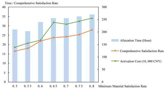
Figure 7.
Objective function values under different minimum material satisfaction rates in Cycle 1.
As the standard of the minimum material satisfaction rate increases, the absolute value of the comprehensive agricultural product satisfaction rate and the sum of distribution center activation costs gradually increase, while the total allocation time fluctuates and remains around 27 to 36 h. Additionally, when the requirement for material security is reduced, the number of activated distribution centers and the sum of their throughput slowly decrease, leading to an increase in the number of demand markets that need distribution services from terminal distribution centers.
The above indicates that to improve the comprehensive satisfaction rate of agricultural products, it is necessary to ensure the minimum satisfaction rate of demand markets. This leads to a simultaneous increase in the allocation volume of agricultural products processed by distribution centers, requiring distribution centers with greater processing capacity. Consequently, this results in higher activation costs and fluctuations in allocation time due to changes in distribution distances. Therefore, to guarantee the satisfaction rate of agricultural products in each demand market and the fairness of material allocation, it is essential to maintain a high standard of minimum material satisfaction rate and activate an appropriate number of distribution centers, ensuring that the material supply–allocation results better meet emergency needs without significantly negative effects on allocation time.
6.3.2. Sensitivity Analysis of Objective Function Weights
To verify the effectiveness of the proposed model and Benders decomposition algorithm, the results are compared by setting the weight coefficients and of the three objective functions as 1 or 0.5, as shown in Table 14. By comparing the magnitudes of the objective function values, it is evident that the upper and lower bounds of (comprehensive satisfaction rate) are . Similarly, the bounds of (allocation time) are , and those of (activation cost) are . It can be inferred that the lower bound of (25.6) occurs when all agricultural products in all demand markets only meet the minimum 80% satisfaction rate. During the material shortage in Cycle 1, the maximum sum of comprehensive satisfaction rates for all demand markets is the upper bound of (27.887). The upper bound of (419) represents the total cost when all distribution centers are activated. As shown in Cases 2, 3 and 6 of Table 14, the lower bounds of and are the extreme values when all demand markets just meet the minimum material satisfaction rate. Furthermore, Case 7 indicates that the upper bound of (27.844) is the comprehensive satisfaction rate under the scheme with the minimum location cost and allocation time. Thus, decision-makers can adjust the weight coefficients to balance the comprehensive satisfaction rate, allocation time, and distribution cost, thereby obtaining optimal allocation–location schemes for different emergency scenarios.
Table 14.
Objective function values under different weight coefficients.
6.3.3. Analysis of Case Scales and Algorithm Performance
To further evaluate the performance of the Benders decomposition algorithm in computational efficiency and solution quality, this section tests six single-cycle cases of varying scales by adjusting the number of agricultural product categories, alternative distribution centers, and demand markets. Cases 1 and 3 represent scenarios with sufficient supply. For robust comparison with the CPLEX solver, each case was executed five times with the results averaged. Detailed outcomes are presented in Table 15 and Table 16, where cases in Table 16 correspond exactly to those in Table 15.
Table 15.
Numerical results for different scale cases.
Table 16.
Performance comparison between the Benders decomposition algorithm and CPLEX.
As the case scale increases, the solution time grows rapidly. Comparing Cases 5 and 6 shows that when the number of agricultural product categories increases, the comprehensive satisfaction rate increases proportionally, while also leading to an increase in total cost and scheduling time. Cases 3 and 4 indicate that a larger number of alternative distribution centers is conducive to finding location schemes with lower total costs. Cases 6 and 7 show that as the number of demand markets increases, the total allocation volume grows, and the number of activated distribution centers correspondingly increases. Cases 1 and 2 demonstrate that the multi-category agricultural product supply–allocation model constructed in this study can also be applied to single-category material allocation problems.
Comparative analysis of the Benders decomposition algorithm and CPLEX solver reveals distinct performance patterns across problem scales. For small-scale cases (e.g., Cases 1, 3, 4), both methods obtain optimal solutions with 0% error rates, though Benders decomposition demonstrates marginal efficiency gains—exemplified by Case 1’s solving time of 1.73 s versus CPLEX’s 2.08 s. As problem complexity escalates, computational times increase substantially for both approaches, yet Benders’ superiority becomes more pronounced: In Case 5, Benders required 36.92 s, achieving approximately 33% time savings over CPLEX (55.38 s). For the most complex case, Case 7, Benders completed in 103.78 s—merely 67% of CPLEX’s 155.67 s—demonstrating enhanced numerical stability when handling high-dimensional variables and intricate constraints.
This divergence likely originates from CPLEX’s full-space search mechanism, which accumulates greater numerical errors than Benders decomposition, with error growth rates accelerating at larger scales. In addition, Benders decomposition mitigates these limitations through primal problem decomposition into master/subproblems and iterative generation of Benders cuts, effectively reducing search dimensionality and floating-point error accumulation. Consequently, via its decomposition strategy and iterative optimization, Benders decomposition delivers both computational efficiency and solution precision for agricultural supply chain models, establishing a dependable computational framework for real-time decision-making scenarios.
Based on empirical findings, we propose the following managerial insights and policy recommendations:
- (1)
- Establish a multi-tiered, dynamically updated agricultural emergency database. Current emergency responses suffer from untimely data collection and inconsistent granularity. We recommend that governments coordinate with agricultural, transportation, commerce departments, and supply chain stakeholders to build a unified database tracking production capacity, real-time inventories, sales volumes, and transportation channel statuses. Standardized daily reporting protocols with minimum granularity requirements should be institutionalized to ensure data authenticity and timeliness for allocation models.
- (2)
- Enhance distribution center planning and emergency activation mechanisms. Simulations confirm that high-throughput, accessible centers critically improve allocation efficiency. Local governments should integrate emergency needs into urban–rural logistics planning by pre-designating alternative centers. Tiered registration systems, activation subsidies, and performance evaluation mechanisms should be implemented to enable rapid resource mobilization during crises.
- (3)
- Develop fairness-constrained allocation assessment frameworks. Incorporating minimum fulfillment rates and max–min fulfillment differentials ensures equitable distribution. Practical emergency systems should adopt such fairness metrics alongside historical allocation records and regional vulnerability indices to guarantee basic supply while enhancing social acceptance of resource distribution, thereby reducing decision-making conflicts and public skepticism.
7. Conclusions
In response to issues such as disrupted production–marketing connections, dynamically changing supply–demand data, and uneven material distribution during sudden disaster events, this study constructs an integrated allocation–location optimization model for emergency agricultural product supply chains based on a rolling horizon approach. The main conclusions are as follows: First, distribution centers are critical nodes influencing the emergency supply of multi-category agricultural products. Their quantity, geographical location, and processing capacity directly determine the efficiency of the allocation system. Case simulations show that systematic location optimization and dynamic adjustment of objective weights can significantly mitigate efficiency losses caused by irrational facility layouts. Moreover, in the event of sudden increases in allocation volume, the model guides the activation of higher-capacity centers, thereby enhancing response flexibility. Second, the rolling-cycle allocation mechanism proposed in this study utilizes dynamically updated production–marketing data and historical shortage information to maximize overall material distribution efficiency while ensuring that all demand markets meet a minimum fulfillment rate. This mechanism significantly improves fairness in cross-cycle allocation, prevents repeated shortages in any single region, reduces material waste, and better aligns with the practical decision-making needs of emergency disaster response.
Nevertheless, although this study has achieved certain theoretical and empirical results, it still has the following limitations:
(1) The model does not account for dynamic uncertainties in transportation, such as road disruptions or reduced traffic efficiency due to severe weather. This may lead to underestimation of actual transportation time and cost, potentially resulting in over-optimistic allocation plans and even delivery failures in extreme scenarios. (2) The assumption that agricultural production and sales data can be shared in a timely manner may overlook the delays and inaccuracies in data collection under disaster conditions, exposing the model to the risk of information lag in practical applications. (3) The model does not incorporate physiological characteristics of agricultural products, such as freshness and ripeness, ignoring quality degradation risks in multi-period scheduling.
To address these limitations, future research could explore the following directions:
- (1)
- Introduce uncertainty modeling techniques, integrate real-time traffic and meteorological data, and develop a robust optimization model under stochastic road disruptions and weather disturbances to enhance system resilience.
- (2)
- Move beyond the current binary framework of supply–demand scenarios by incorporating storage costs and quality losses due to oversupply into the objective function, improving the model’s adaptability to fluctuating markets.
- (3)
- Integrate agricultural product attributes (e.g., freshness decay functions, ripeness thresholds) and cold chain constraints to develop a multi-period quality tracing and loss penalty mechanism.
- (4)
- Promote interdisciplinary methodology integration by combining the current location–allocation framework with technologies such as machine learning and blockchain, extending its application to the scheduling of various perishable goods in humanitarian logistics. For example, IoT-based devices could enable dynamic monitoring of material status, while smart contracts could enhance the transparency and credibility of emergency allocation processes.
Through these improvements, the core framework proposed in this study can evolve into a more universal and practically valuable decision-support tool for emergency management.
Author Contributions
Q.S. conceived and designed the research work; Q.S. and Y.J. wrote the paper together. J.C. validated the model formulation and checked the expression in English. All authors have read and agreed to the published version of the manuscript.
Funding
This research was funded by the National Natural Science Foundation of China [71803084], the Humanity and Social Science Fund of the Ministry of Education of China [22YJA630033], and the Social Science Foundation of Jiangsu Province [21GLC003], XJTLU Research Development Fund [RDF-22-02-010].
Data Availability Statement
The original contributions presented in this study are included in the article. Further inquiries can be directed to the corresponding author.
Conflicts of Interest
The authors declare no conflicts of interest.
References
- Jiang, J.; Ma, J.; Chen, X. Multi-regional collaborative mechanisms in emergency resource reserve and pre-dispatch design. Int. J. Prod. Econ. 2024, 270, 109161. [Google Scholar] [CrossRef]
- Lu, Y.; Sun, S. Scenario-based allocation of emergency resources in metro emergencies: A model development and a case study of Nanjing Metro. Sustainability 2020, 12, 6380. [Google Scholar] [CrossRef]
- Du, Y.; Sun, J.; Duan, Q.; Qi, K.; Xiao, H.; Liew, K.M. Optimal assignments of allocating and scheduling emergency resources to accidents in chemical industrial parks. J. Loss Prev. Process Ind. 2020, 65, 104148. [Google Scholar] [CrossRef]
- Implementation Plan for the 2024 Assessment of District Heads’ Responsibility System for the “Vegetable Basket” Project in Shanghai. Available online: https://nyncw.sh.gov.cn/cmsres/d0/d0836247dc3749ac89ee8af663b47b58/c6598e91b79dc71eea453392c6812059.pdf (accessed on 10 May 2025).
- Ku, A.Y.; Alonso, E.; Eggert, R.; Graedel, T.; Habib, K.; Hool, A.; Kita, Y.; Lee, J.C.; Liu, G.; Nuss, P.; et al. Grand challenges in anticipating and responding to critical materials supply risks. Joule 2024, 8, 1208–1223. [Google Scholar] [CrossRef]
- Zhang, L.; Chu, F.; Zhang, J.; Gu, D. Government decisions for relief materials reserve under supply uncertainty within government-enterprise agreement. Int. J. Prod. Res. 2025, 1–20. [Google Scholar] [CrossRef]
- Xie, K.; Zhu, S.; Gui, P.; Chen, Y. Coordinating an emergency medical material supply chain with CVaR under the pandemic considering corporate social responsibility. Comput. Ind. Eng. 2023, 176, 108989. [Google Scholar] [CrossRef]
- Arabi, M.; Gholamian, M.R.; Teimoury, E.; Mirzamohammadi, S. A robust bi-level programming model to enhance resilience in supply chain network considering government role, taxing, and raw sale: An iron ore case study. Comput. Ind. Eng. 2024, 193, 110322. [Google Scholar] [CrossRef]
- Tian, S.; Mei, Y. Manufacturing security strategies for personal protective equipment in response to the COVID-19 crisis: A regional emergency manufacturing consortium design based on government regulation. IEEE Access 2022, 10, 110947–110959. [Google Scholar] [CrossRef]
- He, J.; Liu, G.; Mai, T.H.T.; Li, T. Research on the allocation of 3D printing emergency supplies in public health emergencies. Front. Public Health 2021, 9, 657276. [Google Scholar] [CrossRef]
- Aron, C.; Sgarbossa, F.; Ballot, E.; Ivanov, D. Cloud material handling systems: A cyber-physical system to enable dynamic resource allocation and digital interoperability. J. Intell. Manuf. 2024, 35, 3815–3836. [Google Scholar] [CrossRef]
- Hao, J.; Li, J.; Wu, D.; Sun, X. Portfolio optimisation of material purchase considering supply risk-A multi-objective programming model. Int. J. Prod. Econ. 2020, 230, 107803. [Google Scholar] [CrossRef]
- Ren, X.; Tan, J. Location allocation collaborative optimization of emergency temporary distribution center under uncertainties. Math. Probl. Eng. 2022, 2022, 6176756. [Google Scholar] [CrossRef]
- Qi, Q.; Tao, F.; Cheng, Y.; Cheng, J.; Nee, A.Y.C. New IT driven rapid manufacturing for emergency response. J. Manuf. Syst. 2021, 60, 928–935. [Google Scholar] [CrossRef] [PubMed]
- Li, T.; Sun, J.; Fei, L. Application of multiple-criteria decision-making technology in emergency decision-making: Uncertainty, heterogeneity, dynamicity, and interaction. Mathematics 2025, 13, 731. [Google Scholar] [CrossRef]
- Fattahi, M.; Govindan, K. A data-driven rolling horizon approach for dynamic design of supply chain distribution networks under disruption and demand uncertainty. Decis. Sci. 2022, 53, 150–180. [Google Scholar] [CrossRef]
- Herding, R.; Mönch, L. A rolling horizon planning approach for short-term demand supply matching. Cent. Eur. J. Oper. Res. 2024, 32, 865–896. [Google Scholar] [CrossRef]
- Lejarza, F.; Venkatesan, S.; Baldea, M. Rolling horizon product quality estimation and online optimisation for supply chain management of perishable inventory. Int. J. Prod. Res. 2025, 63, 3709–3732. [Google Scholar] [CrossRef]
- Sheikholeslami, M.; Zarrinpoor, N. Designing a robust logistics model for perishable emergency commodities in an epidemic outbreak using Lagrangian relaxation: A case of COVID-19. Ann. Oper. Res. 2024, 343, 459–491. [Google Scholar] [CrossRef]
- Hosseini-Motlagh, S.M.; Samani, M.R.G.; Faraji, M. Dynamic optimization of blood collection strategies from different potential donors using rolling horizon planning approach under uncertainty. Comput. Ind. Eng. 2024, 188, 109908. [Google Scholar] [CrossRef]
- Cheng, C.; Chu, H.; Zhang, L.; Tang, L. Green supply chain for steel raw materials under price and demand uncertainty. J. Clean. Prod. 2024, 462, 142621. [Google Scholar] [CrossRef]
- Ghasemi, E.; Lehoux, N.; Rönnqvist, M. A multi-level production-inventory-distribution system under mixed make to stock, make to order, and vendor managed inventory strategies: An application in the pulp and paper industry. Int. J. Prod. Econ. 2024, 271, 109201. [Google Scholar] [CrossRef]
- Fattahi, M.; Keyvanshokooh, E.; Kannan, D.; Govindan, K. Resource planning strategies for healthcare systems during a pandemic. Eur. J. Oper. Res. 2023, 304, 192–206. [Google Scholar] [CrossRef] [PubMed]
- Zhou, Y.; Liu, J.; Zhang, Y.; Gan, X. A multi-objective evolutionary algorithm for multi-period dynamic emergency resource scheduling problems. Transp. Res. Part E Logist. Transp. Rev. 2017, 99, 77–95. [Google Scholar] [CrossRef]
- Cao, C.; Li, C.; Yang, Q.; Liu, Y.; Qu, T. A novel multi-objective programming model of relief distribution for sustainable disaster supply chain in large-scale natural disasters. J. Clean. Prod. 2018, 174, 1422–1435. [Google Scholar] [CrossRef]
- Ruan, J.; Shi, P.; Lim, C.C.; Wang, X. Relief supplies allocation and optimization by interval and fuzzy number approaches. Inf. Sci. 2015, 303, 15–32. [Google Scholar] [CrossRef]
- Liu, J.; Guo, L.; Jiang, J.; Jiang, D.; Wang, P. Emergency material allocation with time-varying supply-demand based on dynamic optimization method for river chemical spills. Environ. Sci. Pollut. Res. 2018, 25, 17343–17353. [Google Scholar] [CrossRef]
- Lee, S.H. A fuzzy multi-objective programming approach for determination of resilient supply portfolio under supply failure risks. J. Purch. Supply Manag. 2017, 23, 211–220. [Google Scholar] [CrossRef]
- Liu, Y.; Li, Y.; Huang, D. A multiobjective optimization model for continuous allocation of emergency rescue materials. Math. Probl. Eng. 2020, 2020, 5693182. [Google Scholar] [CrossRef]
- Li, J.; Zhang, X.; Yao, Y. A bi-level robust optimization model for the coupling allocation of post-disaster personnel and materials assistance. J. Clean. Prod. 2024, 469, 143099. [Google Scholar] [CrossRef]
- Erbeyoğlu, G.; Bilge, Ü. A robust disaster preparedness model for effective and fair disaster response. Eur. J. Oper. Res. 2020, 280, 479–494. [Google Scholar] [CrossRef]
- Hu, X.; Wang, Z.; Zhao, J.; Wang, R.; Lei, H.; Liu, W.; Long, B. Location method for emergency rescue node on expressways based on spatio-temporal characteristics of vehicle operation. Sci. Rep. 2024, 14, 19435. [Google Scholar] [CrossRef]
- Tripathi, G.; Tanksale, A.N.; Verma, M. Optimal location of accident relief facilities in a railway network. Saf. Sci. 2022, 146, 105560. [Google Scholar] [CrossRef]
- Liu, K.; Liu, C.; Xiang, X.; Tian, Z. Testing facility location and dynamic capacity planning for pandemics with demand uncertainty. Eur. J. Oper. Res. 2023, 304, 150–168. [Google Scholar] [CrossRef] [PubMed]
- Li, S.; Han, W.; Liu, L. Robust optimization of the hub location problem for fresh agricultural products with uncertain demand. IEEE Access 2022, 10, 41902–41913. [Google Scholar] [CrossRef]
- Hassanpour, S.T.; Ke, G.Y.; Zhao, J.; Tulett, D.M. Infectious waste management during a pandemic: A stochastic location-routing problem with chance-constrained time windows. Comput. Ind. Eng. 2023, 177, 109066. [Google Scholar] [CrossRef] [PubMed]
- Giusti, R.; Manerba, D.; Crainic, T.G.; Tadei, R. The synchronized multi-commodity multi-service transshipment-hub location problem with cyclic schedules. Comput. Oper. Res. 2023, 158, 106282. [Google Scholar] [CrossRef]
- Li, S.; Zhuang, Y.; Zu, Y.; Liu, L.; Fan, T. Robust cooperative hub location optimization considering demand uncertainty and hub disruptions. Comput. Ind. Eng. 2024, 197, 110591. [Google Scholar] [CrossRef]
- Eydi, A.; Shirinbayan, P. Multi-modal and multi-product hierarchical hub location problem with fuzzy demands. Eng. Appl. Artif. Intell. 2023, 123, 106282. [Google Scholar] [CrossRef]
- Boonmee, C.; Arimura, M.; Asada, T. Facility location optimization model for emergency humanitarian logistics. Int. J. Disaster Risk Reduct. 2017, 24, 485–498. [Google Scholar] [CrossRef]
- Wang, W.; Wu, S.; Wang, S.; Zhen, L.; Qu, X. Emergency facility location problems in logistics: Status and perspectives. Transp. Res. Part E Logist. Transp. Rev. 2021, 154, 102465. [Google Scholar] [CrossRef]
- Shaw, L.; Das, S.K.; Roy, S.K. Location-allocation problem for resource distribution under uncertainty in disaster relief operations. Socio-Econ. Plan. Sci. 2022, 82, 101232. [Google Scholar] [CrossRef]
- Liu, Y.; Cui, N.; Zhang, J. Integrated temporary facility location and casualty allocation planning for post-disaster humanitarian medical service. Transp. Res. Part E Logist. Transp. Rev. 2019, 128, 1–16. [Google Scholar] [CrossRef]
- Geng, J.; Hou, H.; Geng, S. Optimization of warehouse location and supplies allocation for emergency rescue under joint government–enterprise cooperation considering disaster victims’ distress perception. Sustainability 2021, 13, 10560. [Google Scholar] [CrossRef]
- Khayal, D.; Pradhananga, R.; Pokharel, S.; Mutlu, F. A model for planning locations of temporary distribution facilities for emergency response. Socio-Econ. Plan. Sci. 2015, 52, 22–30. [Google Scholar] [CrossRef]
- Vahdani, B.; Veysmoradi, D.; Mousavi, S.M.; Amiri, M. Planning for relief distribution, victim evacuation, redistricting and service sharing under uncertainty. Socio-Econ. Plan. Sci. 2022, 80, 101158. [Google Scholar] [CrossRef]
- Yoruk, E.; Baykasoglu, A.; Avci, M.G. Location and replenishment problems of disaster stations for humanitarian relief logistics along with an application. Nat. Hazards 2023, 119, 1713–1734. [Google Scholar] [CrossRef]
- Sheu, J.B. An emergency logistics distribution approach for quick response to urgent relief demand in disasters. Transp. Res. Part E Logist. Transp. Rev. 2007, 43, 687–709. [Google Scholar] [CrossRef]
- GB/T 38375-2019; Guide for Planning and Design of Food Low Temperature Distribution Center. State Administration for Market Regulation (SAMR): Beijing, China, 2019.
Disclaimer/Publisher’s Note: The statements, opinions and data contained in all publications are solely those of the individual author(s) and contributor(s) and not of MDPI and/or the editor(s). MDPI and/or the editor(s) disclaim responsibility for any injury to people or property resulting from any ideas, methods, instructions or products referred to in the content. |
© 2025 by the authors. Licensee MDPI, Basel, Switzerland. This article is an open access article distributed under the terms and conditions of the Creative Commons Attribution (CC BY) license (https://creativecommons.org/licenses/by/4.0/).