Green’s Function for the Cauchy Problem to the Dissipative Linear Evolution Equation of Arbitrary Order

Abstract

This work addresses the Cauchy problem for a linear equation with a first-order time derivative t and an arbitrary-order spatial derivative x. This equation is a generalization of the linear heat equation of the second order in the case of arbitrary order with respect to spatial variable. The considered linear equation arises from the linearization of the Burgers hierarchy of equations. The Cauchy problem to a linear equation can be solved using the Green function method. The Green function is explicitly constructed for the case of dissipative and dispersive equations and is expressed in terms of generalized hypergeometric functions. The general formulas obtained for representing Green’s function are new. A discussion of specific cases of the equation is also provided.

1. Introduction

In this work, we consider a linear evolution equation of the following form

$$\begin{array}{c}{\Psi }_t+{\alpha }_n{\Psi }_{n+1,x}=0,\end{array}$$

(1)

where ${\Psi }_{n+1,x}={\displaystyle \frac{{\partial }^{n+1}\Psi }{\partial x^{n+1}}},$ $n\in \mathbb{N},$ ${\alpha }_n\in \mathbb{R}.$ The parameter n determines the order of the equation. Equation (1) generalizes the second order linear heat equation to an arbitrary order with respect to the spatial variable. For odd values of n, Equation (1) corresponds to dissipative equations, while for even n, it corresponds to dispersive equations.

Equation (1) is related to the well-known Burgers equation [1,2]. This equation arises from the linearization of the Burgers hierarchy equations

$$\begin{array}{c}{u}_t+{\alpha }_n{\displaystyle \frac{\partial }{\partial x}}{\left({\displaystyle \frac{\partial }{\partial x}}+u\right)}^{n}u=0,n\in \mathbb{N}.\end{array}$$

(2)

Hierarchy (2) was introduced by Olver in 1977 [3]. Equations of this hierarchy find diverse applications in physics [4,5,6,7,8,9]. The first two equations describe viscous incompressible fluid flows, wave phenomena in bubbly liquids, nonlinear acoustic effects, and various other physical processes [10,11,12,13,14]. Additionally, in [15], a fractionally integrable hierarchy of Burgers equations was proposed.

Equation (2) can be transformed into Equation (1) using the Cole–Hopf transformation

$$\begin{array}{c}u={\displaystyle \frac{{\Psi }_x}{\Psi }},\Psi =\Psi (x,t).\end{array}$$

(3)

In the classical works [16,17], the Burgers equation was linearized by means of transformation (3). Later, it was shown that the Cole–Hopf transformation (3) linearizes the entire Burgers hierarchy (2) [18,19]. For this purpose, the authors used the following relation

$$\begin{array}{c}{\left({\displaystyle \frac{\partial }{\partial x}}+{\displaystyle \frac{{\Psi }_x}{\Psi }}\right)}^n{\displaystyle \frac{{\Psi }_x}{\Psi }}={\displaystyle \frac{{\Psi }_{n+1,x}}{\Psi }}.\end{array}$$

(4)

Thus, using Equation (3), we can find the corresponding solution to an equation from the Burgers hierarchy from known solutions of the linear equation.

In this work, we find the Green function for the Cauchy problem to Equation (1) with the initial condition $\varphi \left(x\right)$ [20]. Knowledge of the Green function allows one to find the solution to the Cauchy problem [21,22,23,24,25]. In paper [26], the authors derived an integral representation of the Green function for the Cauchy problem of Equation (1) for arbitrary natural numbers n. Furthermore, explicit forms of the Green function were obtained for specific values of n. Nevertheless, a general formula for Green’s function at an arbitrary value of n has not been established in prior research. This paper presents a general formula for Green’s function for the Cauchy problem of Equation (1) for both even and odd values of n. For $n\ge 2$, Green’s function is expressed in terms of generalized hypergeometric functions.

Generalized hypergeometric functions are represented by the following equality [27,28,29,30]

$$\begin{array}{c}{}_{p}F_q\left(\left[a_1,a_2,\dots ,a_p\right];\left[b_1,b_2\dots ,b_q\right];z\right)={\displaystyle \sum _{k=0}^{\infty }}{\displaystyle \frac{{\displaystyle \prod _{h=1}^p}{\left(a_h\right)}_k{z}^k}{{\displaystyle \prod _{h=1}^q}{\left(b_h\right)}_{k}k!}},\end{array}$$

(5)

where ${\left(a\right)}_k={\displaystyle \frac{\Gamma (a+k)}{\Gamma \left(a\right)}},b_q\ne 0,-1,-2,\dots ,$ quantities $a_1,\dots ,a_p$ and $b_1,\dots ,b_q$ are called the numerator and denominator parameters, respectively, while z is called the argument. The ${}_{p}F_q$ function is symmetric with respect to both the numerator parameters and the denominator parameters. When a numerator parameter coincides with a denominator parameter, these parameters may be canceled, reducing the ${}_{p}F_q$ function to a ${}_{p-1}F_{q-1}$ function. In the absence of numerator parameters, the generalized hypergeometric function (5) is written as ${}_{0}F_q\left(\left[\right];\left[b_1,b_2\dots ,b_q\right];z\right)$.

The aim of this work is to construct the Green function for the Cauchy problem of Equation (1) in both dissipative and dispersive cases, and to derive its explicit expression in terms of generalized hypergeometric functions.

The representation of Green’s function via generalized hypergeometric series offers a number of advantages over the integral representation obtained in [26]. In particular, the representation found in this work allows one to construct a solution to the Cauchy problem for Equation (1) based on the integration formulas for generalized hypergeometric functions [27,28].

The paper is organized as follows. Section 2 formulates the Cauchy problem for the considered equation and presents the solution in integral form using Green’s function. In Section 3, we examine the construction of Green’s function through generalized hypergeometric functions for the dissipative case. Section 4 discusses specific examples illustrating the application of the results for the dissipative case. In Section 5, we provide an explicit representation of Green’s function for the original Cauchy problem in the dispersive case. Section 6 offers concluding remarks.

2. The Cauchy Problem for Equation (1)

The Cauchy problem to Equation (1) takes the form

$$\begin{array}{c}\left\{\begin{array}{c}{\Psi }_t+{\alpha }_n{\Psi }_{n+1,x}=0,-\infty <x<+\infty ,0<t,n\in \mathbb{N},\hfill \\ \Psi (x,0)=\varphi \left(x\right).\hfill \end{array}\right.\end{array}$$

(6)

The function $\varphi \left(x\right)$ belongs to the space of rapidly decreasing functions on $\mathbb{R}.$

This work examines parameter values ${\alpha }_n$ for which Equation (6) solutions remain non-growing with increasing time

$$\begin{array}{c}{\alpha }_n=\left\{\begin{array}{c}{(-1)}^{m+1}{a}^2,a\in \mathbb{R},n=2m,m\in \mathbb{N},\hfill \\ {(-1)}^m{a}^2,a\in \mathbb{R},n=2m-1,m\in \mathbb{N}.\hfill \end{array}\right.\end{array}$$

(7)

For odd values of n ($n=2m-1$), the equations are dissipative in nature, whereas for even ($n=2m$) values of n, they exhibit dispersive behavior.

We construct the solution to problem (6) using the Fourier transform [26]

$$\begin{array}{c}\Psi ={\displaystyle \frac{1}{\sqrt{2\pi }}}\underset{-\infty }{\overset{+\infty }{\int }}f{e}^{i\omega x}d\omega ,\\ f={\displaystyle \frac{1}{\sqrt{2\pi }}}\underset{-\infty }{\overset{+\infty }{\int }}\Psi e^{-i\omega x}dx.\end{array}$$

(8)

Substituting (8) into problem (6), we obtain the Cauchy problem for an equation governing the function f [26]

$$\begin{array}{c}\left\{\begin{array}{c}{f}_t+{\alpha }_n{\left(i\omega \right)}^{n+1}f=0,-\infty <\omega <+\infty ,0<t,n\in \mathbb{N},\hfill \\ f(\omega ,0)=\psi \left(\omega \right)={\displaystyle \frac{1}{\sqrt{2\pi }}}\underset{-\infty }{\overset{+\infty }{\int }}\varphi e^{-i\omega x}dx.\hfill \end{array}\right.\end{array}$$

(9)

The solution to the Cauchy problem (9) has the form

$$\begin{array}{c}f=\psi ·e^{-{\alpha }_n{\left(i\omega \right)}^{n+1}t},\end{array}$$

(10)

and then the function $\Psi$ from Equation (8) will take the form

$$\begin{array}{c}\Psi (x,t)={\displaystyle \frac{1}{2\pi }}\underset{-\infty }{\overset{+\infty }{\int }}\left(\underset{-\infty }{\overset{+\infty }{\int }}\varphi \left(\xi \right)e^{-i\omega \xi -{\alpha }_n{\left(i\omega \right)}^{n+1}t}d\xi \right)e^{i\omega x}d\omega .\end{array}$$

(11)

We reduce Equation (11) to a representation via Green’s function

$$\begin{array}{c}\Psi (x,t)=\underset{-\infty }{\overset{+\infty }{\int }}{G}_n(x,\xi ,t)\varphi \left(\xi \right)d\xi ,\end{array}$$

(12)

where

$$\begin{array}{c}{G}_n(x,\xi ,t)={\displaystyle \frac{1}{2\pi }}\underset{-\infty }{\overset{+\infty }{\int }}{e}^{i\omega (x-\xi )-{\alpha }_n{\left(i\omega \right)}^{n+1}t}d\omega \end{array}$$

(13)

is the Green function.

Since expression (13) admits translation in the x-coordinate, we will consider Equation (13) at $\xi =0$ without loss of generality

$$\begin{array}{c}{G}_n(x,0,t)={\displaystyle \frac{1}{2\pi }}\underset{-\infty }{\overset{+\infty }{\int }}{e}^{i\omega x-{\alpha }_n{\left(i\omega \right)}^{n+1}t}d\omega .\end{array}$$

(14)

Thus, to find the solution to the Cauchy problem (6), we need to compute the integral in the Green function (13) expression for natural values of parameter n. The expressions will differ between the case of odd n and the case of even n.

3. The Green Function for the Cauchy Problem of the Dissipative Equation

In this section, we derive an explicit expression for the Green function (13) in the case $n=2m-1$ and ${\alpha }_n$ from Equation (7) (dissipative case). We represent the expression as a finite sum of generalized hypergeometric functions.

Performing the substitutions $\zeta =\sqrt[2m]{2m{a}^{2}t}\omega ,z={\displaystyle \frac{x}{\sqrt[2m]{2m{a}^{2}t}}}$ in Equation (14), we obtain

$$\begin{array}{c}{G}_{2m-1}(z,0,t)={\displaystyle \frac{1}{2\pi \sqrt[2m]{2m{a}^{2}t}}}\underset{-\infty }{\overset{+\infty }{\int }}{e}^{iz\zeta -{\displaystyle \frac{{\zeta }^{2m}}{2m}}}d\zeta .\end{array}$$

(15)

Next, in Equation (15), we apply Euler’s formula and transform it to integration from 0 to $+\infty$

$$\begin{array}{c}{G}_{2m-1}(z,0,t)={\displaystyle \frac{1}{\pi \sqrt[2m]{2m{a}^{2}t}}}\underset{0}{\overset{+\infty }{\int }}cos\left(z\zeta \right)e^{-{\displaystyle \frac{{\zeta }^{2m}}{2m}}}d\zeta .\end{array}$$

(16)

The problem has been reduced to evaluating the integral

$$\begin{array}{c}{I}_{2m}=\underset{0}{\overset{+\infty }{\int }}cos\left(z\zeta \right)e^{-{\displaystyle \frac{{\zeta }^{2m}}{2m}}}d\zeta .\end{array}$$

(17)

To compute this integral, we employ the Maclaurin series expansion of $cos\left(z\zeta \right)$. Then, Equation (17) transforms to

$$\begin{array}{c}{I}_{2m}={\displaystyle \underset{0}{\overset{+\infty }{\int }}}{\displaystyle \sum _{\beta =0}^{\infty }}{(-1)}^{\beta }{\displaystyle \frac{{\left(z\zeta \right)}^{2\beta }}{\left(2\beta \right)!}}{e}^{-{\displaystyle \frac{{\zeta }^{2m}}{2m}}}d\zeta ={\displaystyle \sum _{\beta =0}^{\infty }}{(-1)}^{\beta }{\displaystyle \frac{z^{2\beta }}{\left(2\beta \right)!}}\underset{0}{\overset{+\infty }{\int }}{\zeta }^{2\beta }{e}^{-{\displaystyle \frac{{\zeta }^{2m}}{2m}}}d\zeta .\end{array}$$

(18)

Consider the inner integral in Equation (18). By making the substitution ${\displaystyle \frac{{\zeta }^{2m}}{2m}}=\eta$, we transform it to a Gamma function

$$\begin{array}{c}\underset{0}{\overset{+\infty }{\int }}{\zeta }^{2\beta }{e}^{-{\displaystyle \frac{{\zeta }^{2m}}{2m}}}d\zeta ={\left(2m\right)}^{{\displaystyle \frac{\beta }{m}}+{\displaystyle \frac{1}{2m}}-1}\underset{0}{\overset{+\infty }{\int }}{\eta }^{{\displaystyle \frac{\beta }{m}}+{\displaystyle \frac{1}{2m}}-1}{e}^{-\eta }d\eta ={\left(2m\right)}^{{\displaystyle \frac{\beta }{m}}+{\displaystyle \frac{1}{2m}}-1}\Gamma \left({\displaystyle \frac{\beta }{m}}+{\displaystyle \frac{1}{2m}}\right).\end{array}$$

(19)

Substituting (19) into (18), we obtain

$$\begin{array}{c}{I}_{2m}={\displaystyle \sum _{\beta =0}^{\infty }}{(-1)}^{\beta }{\displaystyle \frac{z^{2\beta }}{\left(2\beta \right)!}}{\left(2m\right)}^{{\displaystyle \frac{\beta }{m}}+{\displaystyle \frac{1}{2m}}-1}\Gamma \left({\displaystyle \frac{\beta }{m}}+{\displaystyle \frac{1}{2m}}\right)\\ ={\left(2m\right)}^{{\displaystyle \frac{1}{2m}}-1}{\displaystyle \sum _{\beta =0}^{\infty }}{\displaystyle \frac{{(-z^2{\left(2m\right)}^{\frac{1}{m}})}^{\beta }\Gamma \left(\frac{\beta }{m}+\frac{1}{2m}\right)}{\left(2\beta \right)!}}.\end{array}$$

(20)

To compute $I_{2m}$, we now evaluate the series sum by partitioning it into m subseries with indices

$$\begin{array}{c}\beta =mk,\beta =mk+1,\dots ,\beta =mk+l,\dots \beta =mk+m-1,\end{array}$$

(21)

where $l=0,1,\dots ,m-1;k=0,1,2,\dots$

Expression (20) then becomes

$$\begin{array}{c}{I}_{2m}={\left(2m\right)}^{{\displaystyle \frac{1}{2m}}-1}{\displaystyle \sum _{l=0}^{m-1}}{\displaystyle \sum _{k=0}^{\infty }}{\displaystyle \frac{{(-z^2{\left(2m\right)}^{\frac{1}{m}})}^{mk+l}\Gamma \left(k+\frac{l}{m}+\frac{1}{2m}\right)}{\Gamma (2mk+2l+1)}}\\ ={\left(2m\right)}^{{\displaystyle \frac{1}{2m}}-1}{\displaystyle \sum _{l=0}^{m-1}}{\displaystyle \sum _{k=0}^{\infty }}{\displaystyle \frac{{(-z^2{\left(2m\right)}^{\frac{1}{m}})}^{mk+l}\Gamma \left(k+\frac{l}{m}+\frac{1}{2m}\right)}{\Gamma \left(2m\left(k+\frac{l}{m}+\frac{1}{2m}\right)\right)}}.\end{array}$$

(22)

We apply the Gamma function multiplication formula to expression (22)

$$\begin{array}{c}{I}_{2m}={\left(2m\right)}^{{\displaystyle \frac{1}{2m}}-1}{\displaystyle \sum _{l=0}^{m-1}}{\displaystyle \sum _{k=0}^{\infty }}{\displaystyle \frac{{(-z^2{\left(2m\right)}^{\frac{1}{m}})}^{mk+l}\Gamma \left(k+\frac{l}{m}+\frac{1}{2m}\right){\left(2m\right)}^{-(\frac{1}{2}+2mk+2l)}{\left(2\pi \right)}^{\frac{2m-1}{2}}}{\Gamma \left(k+\frac{l}{m}+\frac{1}{2m}\right)·\Gamma \left(k+\frac{l}{m}+\frac{2}{2m}\right)\dots \Gamma \left(k+\frac{l}{m}+\frac{2m}{2m}\right)}}.\end{array}$$

(23)

We cancel the Gamma functions in the numerator and denominator of Equation (23), and introduce $k!$ in both numerator and denominator to reduce the series to a sum of generalized hypergeometric functions

$$\begin{array}{c}{I}_{2m}={\left(2m\right)}^{{\displaystyle \frac{1}{2m}}-1}{\displaystyle \sum _{l=0}^{m-1}}{\displaystyle \sum _{k=0}^{\infty }}{\displaystyle \frac{{(-z^2{\left(2m\right)}^{\frac{1}{m}})}^{mk+l}\Gamma \left(k+1\right){\left(2m\right)}^{-(\frac{1}{2}+2mk+2l)}{\left(2\pi \right)}^{\frac{2m-1}{2}}}{k!·\Gamma \left(k+\frac{l}{m}+\frac{2}{2m}\right)\dots \Gamma \left(k+\frac{l}{m}+\frac{2m}{2m}\right)}}\\ ={\left(2m\right)}^{{\displaystyle \frac{1}{2m}}-{\displaystyle \frac{3}{2}}}{\left(2\pi \right)}^{{\displaystyle \frac{2m-1}{2}}}{\displaystyle \sum _{l=0}^{m-1}}{(-z^2{\left(2m\right)}^{{\displaystyle \frac{1}{m}}-2})}^l{\displaystyle \sum _{k=0}^{\infty }}{\displaystyle \frac{{({(-1)}^m·{\left(2m\right)}^{1-2m}·z^{2m})}^k\Gamma \left(k+1\right)}{k!·\Gamma \left(k+\frac{l}{m}+\frac{2}{2m}\right)\dots \Gamma \left(k+\frac{l}{m}+\frac{2m}{2m}\right)}}\\ ={\left(2m\right)}^{{\displaystyle \frac{1}{2m}}-{\displaystyle \frac{3}{2}}}{\left(2\pi \right)}^{{\displaystyle \frac{2m-1}{2}}}{\displaystyle \sum _{l=0}^{m-1}}{(-z^2{\left(2m\right)}^{{\displaystyle \frac{1}{m}}-2})}^l·{\displaystyle \prod _{\gamma =2}^{2m}}{\displaystyle \frac{1}{\Gamma (\frac{l}{m}+\frac{\gamma }{2m})}}{·}_1{F}_{2m-1}\left(\left[1\right];\right.\\ \left.\left[{\displaystyle \frac{l}{m}}+{\displaystyle \frac{2}{2m}},{\displaystyle \frac{l}{m}}+{\displaystyle \frac{3}{2m}},\dots ,{\displaystyle \frac{l}{m}}+{\displaystyle \frac{2m}{2m}}\right];{(-1)}^m·{\left(2m\right)}^{1-2m}·z^{2m}\right).\end{array}$$

(24)

In this case, Green’s function $G_{2m-1}(x,\xi ,t)$ takes the form

$$\begin{array}{c}{G}_{2m-1}(x,\xi ,t)={\displaystyle \frac{2^{m-2}·{\pi }^{m-\frac{3}{2}}}{m^{\frac{3}{2}}\sqrt[2m]{a^{2}t}}}{\displaystyle \sum _{l=0}^{m-1}}{\left(-{\displaystyle \frac{{(x-\xi )}^2}{4m^2\sqrt[m]{a^{2}t}}}\right)}^l·{\displaystyle \prod _{\gamma =2}^{2m}}{\displaystyle \frac{1}{\Gamma (\frac{l}{m}+\frac{\gamma }{2m})}}\\ {}_{·1}F_{2m-1}\left(\left[1\right];\left[{\displaystyle \frac{l}{m}}+{\displaystyle \frac{2}{2m}},{\displaystyle \frac{l}{m}}+{\displaystyle \frac{3}{2m}},\dots ,{\displaystyle \frac{l}{m}}+{\displaystyle \frac{2m}{2m}}\right];{\displaystyle \frac{1}{a^{2}t}}·{\left(-{\displaystyle \frac{{(x-\xi )}^2}{4m^2}}\right)}^m\right).\end{array}$$

(25)

The generalized hypergeometric function presented by the sum (25) is of the type ${}_{1}F_{2m-1}$. However, by the properties of hypergeometric functions, when a numerator parameter equals a denominator parameter, the function can be expressed with both orders reduced by 1 (as ${}_{0}F_{2m-2}$). In our case, the denominator parameters always include 1 (since $0\le l\le m-1$), meaning that the function could theoretically be reduced to ${}_{0}F_{2m-2}$ form. Nevertheless, for arbitrary m in this work, we retain the original notation for notational convenience.

Using Green’s function (25), the solution to the Cauchy problem (6) is obtained via Formula (12) given the initial condition $\varphi \left(x\right).$

4. Partial Representations of the Green Function

In this section, we examine several special cases of the derived Green’s function Formula (25). For $m=1$, the Cauchy problem (6) is reduced to the Cauchy problem for the linear heat equation

$$\begin{array}{c}\left\{\begin{array}{c}{\Psi }_t=a^2{\Psi }_{xx},-\infty <x<+\infty ,0<t,\hfill \\ \Psi (x,0)=\varphi \left(x\right).\hfill \end{array}\right.\end{array}$$

(26)

The Green function for problem (26) is known [21,22]. We derive it from our Equation (25) as follows.

To accomplish this, we substitute $m=1$ into $I_{2m}$, which yields

$$\begin{array}{c}{I}_2={\left(2\right)}^{-1}{\left(2\pi \right)}^{{\displaystyle \frac{1}{2}}}{\displaystyle \sum _{l=0}^0}{(-z^2{\left(2\right)}^{-1})}^l·{\displaystyle \prod _{\gamma =2}^2}{\displaystyle \frac{1}{\Gamma (l+\frac{\gamma }{2})}}·{}_{1}F_1(\left[1\right];[l+1];(-1)·{\left(2\right)}^{-1}·z^2)\\ \\ =\sqrt{{\displaystyle \frac{\pi }{2}}}{e}^{-{\displaystyle \frac{z^2}{2}}}.\end{array}$$

(27)

In this case, the Green function $G_1$ for the Cauchy problem (26) takes the form

$$\begin{array}{c}{G}_1(x,\xi ,t)={\displaystyle \frac{1}{2a\sqrt{\pi t}}}{e}^{-{\displaystyle \frac{{(x-\xi )}^2}{4a^{2}t}}}.\end{array}$$

(28)

The obtained result (28) agrees with the well-known formula.

Figure 1 illustrates Green’s function $G_1$ (28) at $\xi =0,a=1$ and $t=1$.

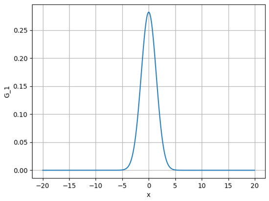
Figure 1. Green’s function $G_1$ (28) at $\xi =0,a=1$ and $t=1$.

Let us consider the Cauchy problem for $m=2$. Then $n=3$, and problem (6) takes the form

$$\begin{array}{c}\left\{\begin{array}{c}{\Psi }_t+a^2{\Psi }_{xxxx}=0,-\infty <x<+\infty ,0<t,\hfill \\ \Psi (x,0)=\varphi \left(x\right).\hfill \end{array}\right.\end{array}$$

(29)

The integral $I_4$ has the form

$$\begin{array}{c}{I}_4={\left(4\right)}^{-{\displaystyle \frac{5}{4}}}{\left(2\pi \right)}^{{\displaystyle \frac{3}{2}}}{\displaystyle \sum _{l=0}^1}{(-z^2{\left(4\right)}^{-{\displaystyle \frac{3}{2}}})}^l·{\displaystyle \prod _{\gamma =2}^4}{\displaystyle \frac{1}{\Gamma (\frac{l}{2}+\frac{\gamma }{4})}}·{}_{1}F_3\left(\left[1\right];\left[{\displaystyle \frac{l}{2}}+{\displaystyle \frac{2}{4}},{\displaystyle \frac{l}{2}}+{\displaystyle \frac{3}{4}},{\displaystyle \frac{l}{2}}+1\right];{\displaystyle \frac{z^4}{64}}\right)\\ ={\displaystyle \frac{\pi }{2\Gamma \left(\frac{3}{4}\right)}}·{}_{0}F_2\left(\left[\right];\left[{\displaystyle \frac{1}{2}},{\displaystyle \frac{3}{4}}\right];{\displaystyle \frac{z^4}{64}}\right)-{\displaystyle \frac{\pi z^2}{2\Gamma \left(\frac{1}{4}\right)}}·{}_{0}F_2\left(\left[\right];\left[{\displaystyle \frac{5}{4}},{\displaystyle \frac{3}{2}}\right];{\displaystyle \frac{z^4}{64}}\right).\end{array}$$

(30)

The Green function for the Cauchy problem (29) is given by the formula

$$\begin{array}{c}{G}_3(x,\xi ,t)={\displaystyle \frac{1}{\sqrt[4]{4a^{2}t}}}·\left({\displaystyle \frac{1}{2\Gamma \left(\frac{3}{4}\right)}}{}_{0}F_2\left(\left[\right];\left[{\displaystyle \frac{1}{2}},{\displaystyle \frac{3}{4}}\right];{\displaystyle \frac{{(x-\xi )}^4}{2^8{a}^{2}t}}\right)\right.\\ \left.-{\displaystyle \frac{{(x-\xi )}^2}{4a\sqrt{t}\Gamma \left(\frac{1}{4}\right)}}{}_{0}F_2\left(\left[\right];\left[{\displaystyle \frac{5}{4}},{\displaystyle \frac{3}{2}}\right];{\displaystyle \frac{{(x-\xi )}^4}{2^8{a}^{2}t}}\right)\right).\end{array}$$

(31)

Figure 2 illustrates Green’s function $G_3$ (31) at $\xi =0,a=1$ and $t=1$.

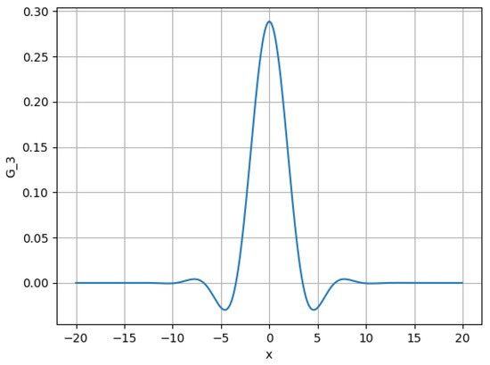
Figure 2. Green’s function $G_3$ (31) at $\xi =0,a=1$ and $t=1$.

For $m=3$ ($n=5$), the Cauchy problem (6) takes the form

$$\begin{array}{c}\left\{\begin{array}{c}{\Psi }_t=a^2{\Psi }_{6,x},-\infty <x<+\infty ,0<t,\hfill \\ \Psi (x,0)=\varphi \left(x\right).\hfill \end{array}\right.\end{array}$$

(32)

In this case, the integral $I_6$ transforms to the form

$$\begin{array}{c}{I}_6={\left(6\right)}^{-{\displaystyle \frac{4}{3}}}{\left(2\pi \right)}^{{\displaystyle \frac{5}{2}}}{\displaystyle \sum _{l=0}^2}{(-z^2{\left(6\right)}^{-{\displaystyle \frac{5}{3}}})}^l·{\displaystyle \prod _{\gamma =2}^6}{\displaystyle \frac{1}{\Gamma (\frac{l}{3}+\frac{\gamma }{6})}}·{}_{1}F_5\left(\left[1\right];\left[{\displaystyle \frac{l}{3}}+{\displaystyle \frac{2}{6}},{\displaystyle \frac{l}{3}}+{\displaystyle \frac{3}{6}},{\displaystyle \frac{l}{3}}+{\displaystyle \frac{4}{6}},{\displaystyle \frac{l}{3}}+{\displaystyle \frac{5}{6}},{\displaystyle \frac{l}{3}}+{\displaystyle \frac{6}{6}}\right];-{\displaystyle \frac{z^6}{6^5}}\right)\\ ={\displaystyle \frac{2^{\frac{1}{6}}\pi }{3^{\frac{5}{6}}\Gamma \left(\frac{5}{6}\right)}}·{}_{0}F_4\left(\left[\right];\left[{\displaystyle \frac{1}{3}},{\displaystyle \frac{1}{2}},{\displaystyle \frac{2}{3}},{\displaystyle \frac{5}{6}}\right];-{\displaystyle \frac{z^6}{6^5}}\right)-{\displaystyle \frac{\sqrt{\pi }{z}^2}{3^{\frac{1}{2}}{2}^{\frac{3}{2}}}}·{}_{0}F_4\left(\left[\right];\left[{\displaystyle \frac{2}{3}},{\displaystyle \frac{5}{6}},{\displaystyle \frac{7}{6}},{\displaystyle \frac{4}{3}}\right];-{\displaystyle \frac{z^6}{6^5}}\right)\\ +{\displaystyle \frac{\pi z^4}{3^{\frac{7}{6}}{2}^{\frac{13}{6}}\Gamma \left(\frac{1}{6}\right)}}·{}_{0}F_4\left(\left[\right];\left[{\displaystyle \frac{7}{6}},{\displaystyle \frac{4}{3}},{\displaystyle \frac{3}{2}},{\displaystyle \frac{5}{3}}\right];-{\displaystyle \frac{z^6}{6^5}}\right)\end{array}$$

(33)

and Green’s function $G_5$ takes the form

$$\begin{array}{c}{G}_5(x,\xi ,t)={\displaystyle \frac{1}{\sqrt[6]{6a^{2}t}}}·\left({\displaystyle \frac{2^{\frac{1}{6}}}{3^{\frac{5}{6}}\Gamma \left(\frac{5}{6}\right)}}·{}_{0}F_4\left(\left[\right];\left[{\displaystyle \frac{1}{3}},{\displaystyle \frac{1}{2}},{\displaystyle \frac{2}{3}},{\displaystyle \frac{5}{6}}\right];-{\displaystyle \frac{{(x-\xi )}^6}{6^6{a}^{2}t}}\right)\right.\\ -{\displaystyle \frac{{(x-\xi )}^2}{{\left(6a^{2}t\right)}^{\frac{1}{3}}\sqrt{\pi }{3}^{\frac{1}{2}}{2}^{\frac{3}{2}}}}·{}_{0}F_4\left(\left[\right];\left[{\displaystyle \frac{2}{3}},{\displaystyle \frac{5}{6}},{\displaystyle \frac{7}{6}},{\displaystyle \frac{4}{3}}\right];-{\displaystyle \frac{{(x-\xi )}^6}{6^6{a}^{2}t}}\right)\\ \left.+{\displaystyle \frac{{(x-\xi )}^4}{{\left(6a^{2}t\right)}^{\frac{2}{3}}{3}^{\frac{7}{6}}{2}^{\frac{13}{6}}\Gamma \left(\frac{1}{6}\right)}}·{}_{0}F_4\left(\left[\right];\left[{\displaystyle \frac{7}{6}},{\displaystyle \frac{4}{3}},{\displaystyle \frac{3}{2}},{\displaystyle \frac{5}{3}}\right];-{\displaystyle \frac{{(x-\xi )}^6}{6^6{a}^{2}t}}\right)\right).\end{array}$$

(34)

Figure 3 illustrates Green’s function $G_5$ (34) at $\xi =0,a=1$ and $t=1$.

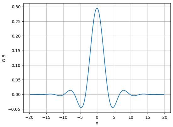
Figure 3. Green’s function $G_5$ (34) at $\xi =0,a=1$ and $t=1$.

Using Formula (25), one can obtain Green’s function for other values of parameter m too.

5. Green’s Function for the Cauchy Problem of the Dispersive Equation

In this section, we derive a representation of the Green function (13) in terms of generalized hypergeometric functions for the case $n=2m$ and ${\alpha }_n$ from Equation (7) (dispersive case).

As the first step, we implement the substitutions $\zeta =\sqrt[2m+1]{(2m+1)a^{2}t}\omega$ and $z={\displaystyle \frac{x}{\sqrt[2m+1]{(2m+1)a^{2}t}}}$ in Equation (14), which yields

$$\begin{array}{c}{G}_{2m}(z,0,t)={\displaystyle \frac{1}{2\pi \sqrt[2m+1]{(2m+1)a^{2}t}}}\underset{-\infty }{\overset{+\infty }{\int }}{e}^{i\left(z\zeta +{\displaystyle \frac{{\zeta }^{2m+1}}{2m+1}}\right)}d\zeta .\end{array}$$

(35)

As the next step, we apply Euler’s formula and then proceed to integrate from 0 to $+\infty$, obtaining

$$\begin{array}{c}{G}_{2m}(z,0,t)={\displaystyle \frac{1}{\pi \sqrt[2m+1]{(2m+1)a^{2}t}}}\underset{0}{\overset{+\infty }{\int }}cos\left(z\zeta +{\displaystyle \frac{{\zeta }^{2m+1}}{2m+1}}\right)d\zeta .\end{array}$$

(36)

Let us examine the resulting integral separately

$$\begin{array}{c}{I}_{2m+1}=\underset{0}{\overset{+\infty }{\int }}cos\left(z\zeta +{\displaystyle \frac{{\zeta }^{2m+1}}{2m+1}}\right)d\zeta .\end{array}$$

(37)

First, applying the cosine addition formula, then expanding both $cos\left(z\zeta \right)$ and $sin\left(z\zeta \right)$ in their Maclaurin series, and subsequently making the substitution $\eta ={\displaystyle \frac{\zeta }{{(2m+1)}^{\frac{1}{2m+1}}}}$, we obtain

$$\begin{array}{c}{I}_{2m+1}=\underset{0}{\overset{+\infty }{\int }}\left(cos\left(z\zeta \right)cos\left({\displaystyle \frac{{\zeta }^{2m+1}}{2m+1}}\right)-sin\left(z\zeta \right)sin\left({\displaystyle \frac{{\zeta }^{2m+1}}{2m+1}}\right)\right)d\zeta \\ =\underset{0}{\overset{+\infty }{\int }}\left({\displaystyle \sum _{\beta =0}^{\infty }}{\displaystyle \frac{{(-1)}^{\beta }{\left(z\zeta \right)}^{2\beta }}{\left(2\beta \right)!}}cos\left({\displaystyle \frac{{\zeta }^{2m+1}}{2m+1}}\right)\right.\\ \left.-{\displaystyle \sum _{\beta =0}^{\infty }}{\displaystyle \frac{{(-1)}^{\beta }{\left(z\zeta \right)}^{2\beta +1}}{(2\beta +1)!}}sin\left({\displaystyle \frac{{\zeta }^{2m+1}}{2m+1}}\right)\right)d\zeta \\ =\underset{0}{\overset{+\infty }{\int }}\left({\displaystyle \sum _{\beta =0}^{\infty }}{\displaystyle \frac{{(-1)}^{\beta }{\left(z\eta \right)}^{2\beta }}{\left(2\beta \right)!}}{(2m+1)}^{{\displaystyle \frac{2\beta +1}{2m+1}}}cos{\eta }^{2m+1}\right.\\ \left.-{\displaystyle \sum _{\beta =0}^{\infty }}{\displaystyle \frac{{(-1)}^{\beta }{\left(z\eta \right)}^{2\beta +1}}{(2\beta +1)!}}{(2m+1)}^{{\displaystyle \frac{2\beta +2}{2m+1}}}sin{\eta }^{2m+1}\right)d\eta .\end{array}$$

(38)

Using the analytic continuation of the Gamma function, we present as follows

$$\begin{array}{c}{I}_{2m+1}={\displaystyle \sum _{\beta =0}^{\infty }}{\displaystyle \frac{{(-1)}^{\beta }{z}^{2\beta }}{\left(2\beta \right)!}}{(2m+1)}^{{\displaystyle \frac{2\beta +1}{2m+1}}-1}\Gamma \left({\displaystyle \frac{2\beta +1}{2m+1}}\right)cos\left({\displaystyle \frac{\pi }{2}}·{\displaystyle \frac{2\beta +1}{2m+1}}\right)\\ -{\displaystyle \sum _{\beta =0}^{\infty }}{\displaystyle \frac{{(-1)}^{\beta }{z}^{2\beta +1}}{(2\beta +1)!}}{(2m+1)}^{{\displaystyle \frac{2\beta +2}{2m+1}}-1}\Gamma \left({\displaystyle \frac{2\beta +2}{2m+1}}\right)sin\left({\displaystyle \frac{\pi }{2}}·{\displaystyle \frac{2\beta +2}{2m+1}}\right).\end{array}$$

(39)

Let us express $I_{2m+1}$ as a sum of two series

$$\begin{array}{c}{I}_{2m+1}=S_1+S_2,\end{array}$$

(40)

where

$$\begin{array}{c}{S}_1={\displaystyle \sum _{\beta =0}^{\infty }}{\displaystyle \frac{{(-1)}^{\beta }{z}^{2\beta }}{\Gamma (2\beta +1)}}{(2m+1)}^{{\displaystyle \frac{2\beta +1}{2m+1}}-1}\Gamma \left({\displaystyle \frac{2\beta +1}{2m+1}}\right)cos\left({\displaystyle \frac{\pi }{2}}·{\displaystyle \frac{2\beta +1}{2m+1}}\right)\end{array}$$

(41)

and

$$\begin{array}{c}{S}_2={\displaystyle \sum _{\beta =0}^{\infty }}{\displaystyle \frac{{(-1)}^{\beta +1}{z}^{2\beta +1}}{\Gamma (2\beta +2)}}{(2m+1)}^{{\displaystyle \frac{2\beta +2}{2m+1}}-1}\Gamma \left({\displaystyle \frac{2\beta +2}{2m+1}}\right)sin\left({\displaystyle \frac{\pi }{2}}·{\displaystyle \frac{2\beta +2}{2m+1}}\right).\end{array}$$

(42)

We transform the series sum $S_1$. Following the approach used in the dissipative case, we partition the series into a sum of $2m+1$ subseries with indices

$$\begin{array}{c}\beta =(2m+1)k,\beta =(2m+1)k+1,\dots ,\beta =(2m+1)k+l,\dots \beta =(2m+1)k+2m,\end{array}$$

(43)

where $l=0,1,\dots ,2m;k=0,1,2,\dots$

Then, expression (41) takes the form

$$\begin{array}{c}{S}_1={\displaystyle \sum _{l=0}^{2m}}{\displaystyle \sum _{k=0}^{\infty }}{\displaystyle \frac{{(-z^2)}^{(2m+1)k+l}{(2m+1)}^{\frac{2(2m+1)k+2l+1}{2m+1}-1}\Gamma \left(\frac{2(2m+1)k+2l+1}{2m+1}\right)}{\Gamma \left(2\right(2m+1)k+2l+1)}}\\ ·cos\left({\displaystyle \frac{\pi }{2}}·{\displaystyle \frac{2(2m+1)k+2l+1}{2m+1}}\right)={\displaystyle \sum _{l=0}^{2m}}{(-z^2)}^l{(2m+1)}^{{\displaystyle \frac{2l+1}{2m+1}}-1}\\ ·\left({\displaystyle \sum _{k=0}^{\infty }}{\displaystyle \frac{{(-z^2)}^{(2m+1)k}{(2m+1)}^{2k}\Gamma \left(2k+\frac{2l+1}{2m+1}\right)cos\left(\frac{\pi }{2}·\left(2k+\frac{2l+1}{2m+1}\right)\right)}{\Gamma \left(2\right(2m+1)k+2l+1)}}\right).\end{array}$$

(44)

We apply Gauss’s multiplication formula for the Gamma function in Equation (44) to both the numerator and denominator, then reduce the expression to a sum of generalized hypergeometric functions. As a result, the inner series in Equation (44) takes the form

$$\begin{array}{c}{\displaystyle \sum _{k=0}^{\infty }}{\displaystyle \frac{{(-z^2)}^{(2m+1)k}{(2m+1)}^{2k}\Gamma \left(k+\frac{2l+1}{2(2m+1)}\right)\Gamma \left(k+\frac{2l+1}{2(2m+1)}+\frac{1}{2}\right)}{\Gamma \left(k+\frac{2l+1}{2(2m+1)}\right)\dots \Gamma \left(k+\frac{2l+1}{2(2m+1)}+\frac{2(2m+1)-1}{2(2m+1)}\right)2^{1-\left(2k+\frac{2l+1}{2m+1}\right)}}}·{\displaystyle \frac{cos\left(\frac{\pi }{2}·\left(2k+\frac{2l+1}{2m+1}\right)\right){\left(2\pi \right)}^{2m+\frac{1}{2}}}{\sqrt{\pi }{\left(2(2m+1)\right)}^{2(2m+1)k+2l+\frac{1}{2}}}}\\ ={\displaystyle \frac{{\pi }^{2m}cos(\frac{\pi }{2}·\frac{2l+1}{2m+1})}{2^{2l-2m-\frac{2l+1}{2m+1}+1}{(2m+1)}^{2l+\frac{1}{2}}}}·{\displaystyle \sum _{k=0}^{\infty }}{\displaystyle \frac{z^{2(2m+1)k}\Gamma (k+1)\Gamma \left(k+\frac{2l+1}{2(2m+1)}+\frac{1}{2}\right)}{{k!(4m+2))}^{4mk}\Gamma \left(k+\frac{2l+2}{2(2m+1)}\right)..\Gamma \left(k+\frac{2l+2(2m+1)}{2(2m+1)}\right)}}\\ ={\displaystyle \frac{{\pi }^{2m}cos\left(\frac{\pi }{2}·\frac{2l+1}{2m+1}\right)}{2^{2l-2m-\frac{2l+1}{2m+1}+1}{(2m+1)}^{2l+\frac{1}{2}}}}\Gamma \left({\displaystyle \frac{2l+1}{2(2m+1)}}+{\displaystyle \frac{1}{2}}\right)·{\displaystyle \prod _{\gamma =2}^{2(2m+1)}}{\displaystyle \frac{1}{\Gamma \left(\frac{2l+\gamma }{2(2m+1)}\right)}}\\ {·}_2{F}_{4m+1}\left(\left[1,{\displaystyle \frac{2l+1}{2(2m+1)}}+{\displaystyle \frac{1}{2}}\right];\left[{\displaystyle \frac{2l+2}{2(2m+1)}},\dots ,{\displaystyle \frac{2l+2(2m+1)}{2(2m+1)}}\right];{\displaystyle \frac{z^{2(2m+1)}}{{\left(2(2m+1)\right)}^{4m}}}\right).\end{array}$$

(45)

The sum $S_1$ takes the form

$$\begin{array}{c}{S}_1={\displaystyle \sum _{l=0}^{2m}}{(-z^2)}^l{\displaystyle \frac{{\pi }^{2m}cos(\frac{\pi }{2}·\frac{2l+1}{2m+1})}{2^{2l-2m-\frac{2l+1}{2m+1}+1}{(2m+1)}^{2l+\frac{3}{2}-\frac{2l+1}{2m+1}}}}\Gamma \left({\displaystyle \frac{2l+1}{2(2m+1)}}+{\displaystyle \frac{1}{2}}\right)·{\displaystyle \prod _{\gamma =2}^{2(2m+1)}}{\displaystyle \frac{1}{\Gamma \left(\frac{2l+\gamma }{2(2m+1)}\right)}}·\\ {·}_2{F}_{4m+1}\left(\left[1,{\displaystyle \frac{2l+1}{2(2m+1)}}+{\displaystyle \frac{1}{2}}\right];\left[{\displaystyle \frac{2l+2}{2(2m+1)}},\dots ,{\displaystyle \frac{2l+2(2m+1)}{2(2m+1)}}\right];{\displaystyle \frac{z^{2(2m+1)}}{{\left(2(2m+1)\right)}^{4m}}}\right).\end{array}$$

(46)

Using the same steps as for the sum $S_1$, we now perform the analogous procedure for the series $S_2$. We partition the series into a sum of $2m+1$ subseries with indices

$$\begin{array}{c}\beta =(2m+1)k,\beta =(2m+1)k+1,\dots ,\beta =(2m+1)k+l,\dots \beta =(2m+1)k+2m,\end{array}$$

(47)

where $l=0,1,\dots ,2m;k=0,1,2,\dots$

Then, Equation (42) takes the form

$$\begin{array}{c}{S}_2={\displaystyle \sum _{l=0}^{2m}}{\displaystyle \sum _{k=0}^{\infty }}{\displaystyle \frac{{(-1)}^{(2m+1)k+l+1}{z}^{2(2m+1)k+2l+1}{(2m+1)}^{\frac{2(2mk+k+l+1)}{2m+1}-1}}{\Gamma \left(2\right(2m+1)k+2l+2)}}\\ ·\Gamma \left({\displaystyle \frac{2(2mk+k+l+1)}{2m+1}}\right)sin\left({\displaystyle \frac{\pi }{2}}·{\displaystyle \frac{2(2mk+k+l+1)}{2m+1}}\right)\\ ={\displaystyle \sum _{l=0}^{2m-1}}{(-1)}^{l+1}{z}^{2l+1}{(2m+1)}^{{\displaystyle \frac{2l+2}{2m+1}}-1}sin\left({\displaystyle \frac{\pi }{2}}·{\displaystyle \frac{2l+2}{2m+1}}\right)\\ ·\left({\displaystyle \sum _{k=0}^{\infty }}{\displaystyle \frac{z^{2(2m+1)k}{(2m+1)}^{2k}\Gamma \left(2k+\frac{2l+2}{2m+1}\right)}{\Gamma \left(2(2m+1)\left(k+\frac{2l+2}{2(2m+1)}\right)\right)}}\right).\end{array}$$

(48)

Then, we reduce the inner series in Equation (48) to generalized hypergeometric functions

$$\begin{array}{c}{\displaystyle \sum _{k=0}^{\infty }}{\displaystyle \frac{z^{2(2m+1)k}{(2m+1)}^{2k}\Gamma \left(k+\frac{2l+2}{2(2m+1)}\right)\Gamma \left(k+\frac{2l+2}{2(2m+1)}+\frac{1}{2}\right)}{2^{1-2k-\frac{2l+2}{2m+1}}\sqrt{\pi }\Gamma \left(k+\frac{2l+2}{2(2m+1)}\right)\dots \Gamma \left(k+\frac{2l+2}{2(2m+1)}+\frac{2(2m+1)-1}{2(2m+1)}\right)}}·{\displaystyle \frac{{\left(2\pi \right)}^{2m+\frac{1}{2}}}{{\left(2(2m+1)\right)}^{\frac{3}{2}+2(2m+1)k+2l}}}\\ ={\displaystyle \frac{2^{2m-2l-2+\frac{2l+2}{2m+1}}{\pi }^{2m}}{{(2m+1)}^{2l+\frac{3}{2}}}}·{\displaystyle \sum _{k=0}^{\infty }}{\displaystyle \frac{z^{2(2m+1)k}\Gamma (k+1)\Gamma \left(k+\frac{2l+2}{2(2m+1)}+\frac{1}{2}\right)}{{\left(2(2m+1)\right)}^{4mk}k!·\Gamma \left(k+\frac{2l+3}{2(2m+1)}\right)\dots \Gamma \left(k+\frac{2l+2(2m+1)+1}{2(2m+1)}\right)}}\\ ={\displaystyle \frac{2^{2m-2l-2+\frac{2l+2}{2m+1}}{\pi }^{2m}}{{(2m+1)}^{2l+\frac{3}{2}}}}\Gamma \left({\displaystyle \frac{2l+2}{2(2m+1)}}+{\displaystyle \frac{1}{2}}\right)·{\displaystyle \prod _{\gamma =3}^{2(2m+1)+1}}{\displaystyle \frac{1}{\Gamma \left(\frac{2l+\gamma }{2(2m+1)}\right)}}\\ {·}_2{F}_{4m+1}\left(\left[1,{\displaystyle \frac{2l+2}{2(2m+1)}}+{\displaystyle \frac{1}{2}}\right];\left[{\displaystyle \frac{2l+3}{2(2m+1)}},\dots ,{\displaystyle \frac{2l+2(2m+1)+1}{2(2m+1)}}\right];{\displaystyle \frac{z^{2(2m+1)}}{{\left(2(2m+1)\right)}^{4m}}}\right).\end{array}$$

(49)

We have the final expression for the sum $S_2$ in the form

$$\begin{array}{c}{S}_2={\displaystyle \sum _{l=0}^{2m-1}}{(-1)}^{l+1}{z}^{2l+1}sin\left({\displaystyle \frac{\pi }{2}}·{\displaystyle \frac{2l+2}{2m+1}}\right){\displaystyle \frac{2^{2m-2l-2+\frac{2l+2}{2m+1}}{\pi }^{2m}\Gamma \left(\frac{2l+2}{2(2m+1)}+\frac{1}{2}\right)}{{(2m+1)}^{2l+\frac{5}{2}-\frac{2l+2}{2m+1}}}}\\ ·{\displaystyle \prod _{\gamma =3}^{2(2m+1)+1}}{\displaystyle \frac{1}{\Gamma \left(\frac{2l+\gamma }{2(2m+1)}\right)}}{·}_2{F}_{4m+1}\left(\left[1,{\displaystyle \frac{2l+2}{2(2m+1)}}+{\displaystyle \frac{1}{2}}\right];\right.\\ \left.\left[{\displaystyle \frac{2l+3}{2(2m+1)}},\dots ,{\displaystyle \frac{2l+2(2m+1)+1}{2(2m+1)}}\right];{\displaystyle \frac{z^{2(2m+1)}}{{\left(2(2m+1)\right)}^{4m}}}\right).\end{array}$$

(50)

We also note that the generalized hypergeometric function ${}_{2}F_{4m+1}$ in $S_1$ and $S_2$ can be reduced to ${}_{0}F_{4m-1}$ function, if required.

Now, with $S_1$ and $S_2$ determined, we express $I_{2m+1}$ as

$$\begin{array}{c}{I}_{2m+1}={\displaystyle \sum _{l=0}^{2m}}{(-z^2)}^l{\displaystyle \frac{{\pi }^{2m}cos(\frac{\pi }{2}·\frac{2l+1}{2m+1})}{2^{2l-2m-\frac{2l+1}{2m+1}+1}{(2m+1)}^{2l+\frac{3}{2}-\frac{2l+1}{2m+1}}}}\Gamma \left({\displaystyle \frac{2l+1}{2(2m+1)}}+{\displaystyle \frac{1}{2}}\right)\\ ·{\displaystyle \prod _{\gamma =2}^{2(2m+1)}}{\displaystyle \frac{1}{\Gamma \left(\frac{2l+\gamma }{2(2m+1)}\right)}}{·}_2{F}_{4m+1}\left(\left[1,{\displaystyle \frac{2l+1}{2(2m+1)}}+{\displaystyle \frac{1}{2}}\right];\right.\\ \left.\left[{\displaystyle \frac{2l+2}{2(2m+1)}},\dots ,{\displaystyle \frac{2l+2(2m+1)}{2(2m+1)}}\right];{\displaystyle \frac{z^{2(2m+1)}}{{\left(2(2m+1)\right)}^{4m}}}\right)\\ +{\displaystyle \sum _{l=0}^{2m-1}}{(-1)}^{l+1}{z}^{2l+1}sin\left({\displaystyle \frac{\pi }{2}}·{\displaystyle \frac{2l+2}{2m+1}}\right){\displaystyle \frac{2^{2m-2l-2+\frac{2l+2}{2m+1}}{\pi }^{2m}\Gamma \left(\frac{2l+2}{2(2m+1)}+\frac{1}{2}\right)}{{(2m+1)}^{2l+\frac{5}{2}-\frac{2l+2}{2m+1}}}}\\ ·{\displaystyle \prod _{\gamma =3}^{2(2m+1)+1}}{\displaystyle \frac{1}{\Gamma \left(\frac{2l+\gamma }{2(2m+1)}\right)}}{·}_2{F}_{4m+1}\left(\left[1,{\displaystyle \frac{2l+2}{2(2m+1)}}+{\displaystyle \frac{1}{2}}\right];\right.\\ \left.\left[{\displaystyle \frac{2l+3}{2(2m+1)}},\dots ,{\displaystyle \frac{2l+2(2m+1)+1}{2(2m+1)}}\right];{\displaystyle \frac{z^{2(2m+1)}}{{\left(2(2m+1)\right)}^{4m}}}\right).\end{array}$$

(51)

From the computed integral (51), we obtain the expression for the Green function $G_{2m}$, which takes the form

$$\begin{array}{c}{G}_{2m}(x,\xi ,t)={\displaystyle \frac{1}{\pi \sqrt[2m+1]{(2m+1)a^{2}t}}}\left({\displaystyle \sum _{l=0}^{2m}}{\left(-{\left({\displaystyle \frac{x-\xi }{{\left((2m+1)a^{2}t\right)}^{\frac{1}{2m+1}}}}\right)}^2\right)}^l\right.\\ ·{\displaystyle \frac{{\pi }^{2m}cos\left(\frac{\pi }{2}·\frac{2l+1}{2m+1}\right)}{2^{2l-2m-\frac{2l+1}{2m+1}+1}{(2m+1)}^{2l+\frac{3}{2}-\frac{2l+1}{2m+1}}}}\Gamma \left({\displaystyle \frac{2l+1}{2(2m+1)}}+{\displaystyle \frac{1}{2}}\right)·{\displaystyle \prod _{\gamma =2}^{2(2m+1)}}{\displaystyle \frac{1}{\Gamma \left(\frac{2l+\gamma }{2(2m+1)}\right)}}\\ {·}_2{F}_{4m+1}\left(\left[1,{\displaystyle \frac{2l+1}{2(2m+1)}}+{\displaystyle \frac{1}{2}}\right];\left[{\displaystyle \frac{2l+2}{2(2m+1)}},\dots ,{\displaystyle \frac{2l+2(2m+1)}{2(2m+1)}}\right];\right.\\ \left.{\displaystyle \frac{{(x-\xi )}^{4m+2}}{2^{4m}{a}^4{t}^2{(2m+1)}^{4m+2}}}\right)+{\displaystyle \sum _{l=0}^{2m-1}}{(-1)}^{l+1}{\left({\displaystyle \frac{x-\xi }{{\left((2m+1)a^{2}t\right)}^{\frac{1}{2m+1}}}}\right)}^{2l+1}\\ ·sin\left({\displaystyle \frac{\pi }{2}}·{\displaystyle \frac{2l+2}{2m+1}}\right){\displaystyle \frac{2^{2m-2l-2+\frac{2l+2}{2m+1}}{\pi }^{2m}\Gamma \left(\frac{2l+2}{2(2m+1)}+\frac{1}{2}\right)}{{(2m+1)}^{2l+\frac{5}{2}-\frac{2l+2}{2m+1}}}}\\ ·{\displaystyle \prod _{\gamma =3}^{2(2m+1)+1}}{\displaystyle \frac{1}{\Gamma \left(\frac{2l+\gamma }{2(2m+1)}\right)}}{·}_2{F}_{4m+1}\left(\left[1,{\displaystyle \frac{2l+2}{2(2m+1)}}+{\displaystyle \frac{1}{2}}\right];\right.\\ \left.\left.\left[{\displaystyle \frac{2l+3}{2(2m+1)}},\dots ,{\displaystyle \frac{2l+2(2m+1)+1}{2(2m+1)}}\right];{\displaystyle \frac{{(x-\xi )}^{4m+2}}{2^{4m}{a}^4{t}^2{(2m+1)}^{4m+2}}}\right)\right).\end{array}$$

(52)

Using the obtained Green’s function (52), one can find the solution to the Cauchy problem (6) for a given function $\varphi \left(x\right).$

6. Conclusions

In this paper, we have constructed the Cauchy problem for a linear evolutionary equation of arbitrary order, arising from the linearization of the Burgers hierarchy. The main focus is on constructing Green’s function for this equation in both dissipative and dispersive cases. The obtained results allow us to express the solution of the Cauchy problem explicitly through an integral representation using Green’s function, significantly expanding the possibilities for analyzing such equations. One of the key achievements of this work is the explicit representation of Green’s function as a finite sum of generalized hypergeometric functions. It is shown that in special cases, such as the heat equation, the derived formulas agree with known results. The use of properties of special functions, such as the gamma function and generalized hypergeometric functions, has enabled the derivation of compact and analytically convenient expressions.

The results of this work open new avenues for studying the asymptotic behavior of solutions, their stability, and other properties. Additionally, the obtained Green’s functions may be useful for further research in mathematical physics. In particular, these results can be used to construct solutions for the Burgers hierarchy equations. Furthermore, the proposed approach can be adapted for analyzing other classes of linear and nonlinear evolutionary equations.

References

- Bateman, H. Some Recent Researches on the Motion of Fluids. Mon. Rev. 1915, 43, 163–170. [Google Scholar] [CrossRef]
- Burgers, J.M. A mathematical model illustrating the theory turbulence. Adv. Appl. Mech. 1948, 1, 171–199. [Google Scholar]
- Olver, P.J. Evolution equations possessing infinitely many symmetries. J. Math. Phys. 1977, 18, 1212–1215. [Google Scholar] [CrossRef]
- Sharma, V.D.; Madhumita, G.; Manickam, S.A.V. Dissipative waves in a relaxing gas exhibiting mixed nonlinearity. Nonlinear Dyn. 2003, 33, 283–299. [Google Scholar] [CrossRef]
- Ibragimov, N.H.; Kolsrud, T. Lagrangian approach to evolution equations: Symmetries and conservation laws. Nonlinear Dyn. 2004, 36, 29–40. [Google Scholar] [CrossRef]
- Qian, C.Z.; Tang, J.S. Asymptotic solution for a kind of boundary layer problem. Nonlinear Dyn. 2006, 45, 15–24. [Google Scholar] [CrossRef]
- Biswas, A.; Triki, H.; Hayat, T.; Aldossary, O.M. 1-Soliton solution of the generalized Burgers equation with generalized evolution. Appl. Math. Comput. 2011, 217, 10289–10294. [Google Scholar] [CrossRef]
- Boritchev, A. Estimates for solutions of a low-viscosity kick-forced generalized Burgers equation. Proc. R. Soc. Edinb. A 2013, 143, 253–263. [Google Scholar] [CrossRef]
- Lou, S. Progresses on Some Open Problems Related to Infinitely Many Symmetries. Mathematics 2024, 12, 3224. [Google Scholar] [CrossRef]
- Kraenkel, R.A.; Pereira, J.G.; de Rey Neto, E.C. Linearizability of the perturbed Burgers equation. Phys. Rev. E 1998, 58, 2526–2530. [Google Scholar] [CrossRef]
- Billingham, J.; King, A.C. Wave Motion; Cambridge University Press: Cambridge, MA, USA, 2000; Volume 468. [Google Scholar]
- Fokas, T.S.; Luo, L. On the asymptotic linearization of acoustic waves. Trans. Am. Math. 2008, 360, 6403–6445. [Google Scholar] [CrossRef][Green Version]
- Kudryashov, N.A.; Sinelshchikov, D.I. An extended equation for the description of nonlinear waves in a liquid with gas bubbles. Wave Motion 2013, 50, 351–362. [Google Scholar] [CrossRef]
- Kudryashov, N.A.; Sinelshchikov, D.I.; Soukharev, M.B. Higher order equations for the description of wave process in liquid with gas bubbles. Vest. NRNU MEPhI. 2013, 2, 142–151. [Google Scholar]
- Ablowitz, M.; Nixon, S. Integrable fractional Burgers hierarchy. J. Nonlinear Waves 2025, 1, e3. [Google Scholar] [CrossRef]
- Hopf, E. The partial differential equation ut + u ux = uxx. Commun. Pure Appl. Math. 1950, 3, 201–230. [Google Scholar] [CrossRef]
- Cole, J.D. On a quasi-linear parabolic equation occuring in aerodynamics. Q. Appl. Math. 1951, 3, 225–236. [Google Scholar] [CrossRef]
- Kudryashov, N.A.; Sinelshchikov, D.I. Exact solutions of equations for the Burgers hierarchy. Appl. Math. Comput. 2009, 215, 1293–1300. [Google Scholar] [CrossRef]
- Kudryashov, N.A. Solitary Waves of Burgers Hierarchy Equations. Comput. Math. Math. 2025, 65, 995–1003. [Google Scholar] [CrossRef]
- Whitham, G.B. Linear and Nonlinear Waves; Jhon Wiley and Sons: New York, NY, USA; London, UK; Sydney, Australia; Toronto, ON, Canada, 1974. [Google Scholar]
- Butkovskiy, A.G. Green’s Functions and Transfer Functions Handbook; Halstead Press–John Wiley and Sons: New York, NY, USA, 1982. [Google Scholar]
- Polyanin, A.D.; Zaitsev, V.F.; Zhyrov, A.I. Methods of Nonlinear Equations of Mathematical Physics and Mechanics; Fizmatlit: Moscow, Russia, 2005. [Google Scholar]
- Cole, K.D.; Beck, J.V.; Haji-Sheikh, A.; Litkouhi, B. Methods for Obtaining Green’s Functions. In Heat Conduction Using Greens Functions; CRC Press: Boca Raton, FL, USA, 2010; Volume 4, pp. 101–148. [Google Scholar]
- Polyanin, A.D.; Zaitsev, V.F. Handbook of Nonlinear Partial Differential Equations, 2nd ed.; Chapman and Hall/CRC: London, UK; Boca Raton, FL, USA, 2011. [Google Scholar]
- Polyanin, A.D.; Nazaikinskii, V.E. Handbook of Linear Partial Differential Equations for Engineers and Scientists; Chapman and Hall/CRC: New York, NY, USA, 2016. [Google Scholar]
- Kudryashov, N.A.; Sinelshchikov, D.I. The Cauchy problem for the equation of the Burgers hierarchy. Nonlinear Dyn. 2014, 76, 561–569. [Google Scholar] [CrossRef]
- Dunaev, A.S.; Shlychkov, V.I. Hypergeometric Functions; Ural Federal University: Yekaterinburg, Russia, 2017. [Google Scholar]
- Rao, K.S.; Lakshminarayanan, V. Generalized Hypergeometric Functions; IOP Publishing: Bristol, UK, 2018. [Google Scholar]
- Srivastava, H.M.; Manocha, H.L. A Treatise on Generating Functions; Halsted Press (Ellis Horwood Limited): Chichester, UK; John Wiley & Sons: New York, NY, USA, 1984. [Google Scholar]
- Srivastava, H.M.; Arjika, S. A General Family of q-Hypergeometric Polynomials and Associated Generating Functions. Mathematics 2021, 9, 1161. [Google Scholar] [CrossRef]
Disclaimer/Publisher’s Note: The statements, opinions and data contained in all publications are solely those of the individual author(s) and contributor(s) and not of MDPI and/or the editor(s). MDPI and/or the editor(s) disclaim responsibility for any injury to people or property resulting from any ideas, methods, instructions or products referred to in the content. |
© 2025 by the authors. Licensee MDPI, Basel, Switzerland. This article is an open access article distributed under the terms and conditions of the Creative Commons Attribution (CC BY) license (https://creativecommons.org/licenses/by/4.0/).