Abstract
Understanding and modeling the effect of magnetic fields on flows that present separation properties, such as those over a backward-facing step (BFS), is critical due to its role in metallurgical processes, nuclear reactor cooling, plasma confinement, and biomedical applications. This study examines the hydrodynamic and magnetohydrodynamic numerical solution of an electrically conducting fluid flow in a backward-facing step (BFS) geometry under the influence of an external, uniform magnetic field applied at an angle. The novelty of this work lies in employing an in-house finite-volume solver with a collocated grid configuration that directly applies a Newton–like method, in contrast to conventional iterative approaches. The computed hydrodynamic results are validated with experimental and numerical studies for an expansion ratio of two, while the MHD case is validated for Reynolds number and Stuart number . One of the most important findings is the reduction in the reattachment point and simultaneous increase in pressure as the magnetic field strength is amplified. The magnetic field angle with the greatest influence is observed at , where the main recirculation vortex is substantially suppressed. These results not only clarify the role of magnetic field orientation in BFS flows but also lay the foundation for future investigations of three-dimensional configurations and coupled MHD–thermal applications.
Keywords:
backward-facing step; magnetohydrodynamics; finite volumes method; direct numerical solution; point of flow reattachment MSC:
35Q30; 65N08; 76W05
1. Introduction
The backward-facing step (BFS), also referenced in the literature as “sudden expansion flow” or “backward flow”, constitutes a classic benchmark problem in Computational Fluid Dynamics (CFDs). Its significance arises from its ability to model separated flows. The flow downstream of the step point presents the separation bubble formation and reattachment processes in both the lower and upper walls. For a high Reynolds number (), multiple bubbles exist in both walls. Reattachment and separation points are highly affected by geometry, inlet–outlet boundary conditions, and heat transfer. Many numerical studies have been conducted for the investigation of the effects of the outflow boundary conditions in the BFS flow, such as Papanastasiou et al. and Gartling who highlighted the importance of such boundary conditions in the numerical solution [1,2]. Examining these flows is vital due to the various real-life applications such as the flow behind airfoils at large angles of attack, or spoiler flows [3]. Separation is a phenomenon that scientists try to avoid as it leads to flow resistance and consequently to large energy losses.
The flow over a BFS has been established as a test problem to challenge the accuracy of numerical methods, due to the dependence of the reattachment length, on the Reynolds number and the expansion ratio (ER) [4]. Numerous studies compared their numerical findings with experimental data, such as those of Armaly et al. [5] for ER = 1.942, whereas Lee and Mateescu studied for BFS ER = 1.17 and ER = 2.0 [6]. These efforts aim to achieve accurate predictions of the reattachment point. The fundamental quantity that validates the accuracy of the method is the reattachment point of the bubble on both walls. The three-dimensional nature of the problem affects the comparison of the reattachment point in both walls, regarding two-dimensional numerical studies and three-dimensional experimental data, as Armaly et al. indicate [5]. The agreement among numerical studies with experimental data are still not satisfactory and it is highlighted that the extra third dimension drastically affects the reattachment distance when [7,8].
As the flow separates at the corner of the step, a recirculation region forms downstream and the flow reattaches at distance from the corner step. For a large Reynolds number, additional separation and recirculation points appear in the upper wall. As increases, multiple recirculation regions emerge in both the upper and lower walls [9]. This behavior is attributed to the adverse pressure gradient associated with the expanding flow, created by a sudden change in the cross-section [10].
The case of a two-dimensional, steady-state incompressible flow over a BFS has been thoroughly examined for a small Reynolds number. The main concern of scientists is the investigation of BFS flows over due to the controversy on whether it is possible to obtain a stable solution. The is believed to be the upper regime to obtain a stable numerical solution [9]. The turbulent BFS flow has been studied meticulously by scientists; consequently, numerical and experimental calculations have established the transitional regime to be for [6]. Numerous studies have been conducted in a turbulent case as that described by Erturk, Liakos and Malamataris and Choi et al. investigating the transitional regions and bifurcations that occur in two- or three-dimensional fluid flows [9,11,12]. Recent studies on 3D BFS flows have examined thermal performance, focusing on how geometric changes like downstream baffles affect heat transfer. Parameters such as baffle height, thickness, and position significantly influence flow and Nusselt number distribution across varying Reynolds and Grashof numbers [13].
The primary distance reattachment point is a function of the expansion rate () and the Reynolds number (). In this study, , is based on the height H, of the channel, , where defined as the average value of the inlet velocity, or else the of . In the case of ER = 2.0, is identical with, , where D is the hydraulic diameter defined as twice the height of the inlet region upstream of the geometry (). In the scope of this study, the expansion rate is selected at 2.0 because it is the most studied case in the literature and facilitates comparison. As the expansion rate increases, the reattachment point decreases as Erturk presents in [9]. The geometry of BFS has a dimensionless length of , height of , the step height is . Consequently, the expansion ratio is equal to 2.0 and the step location on the x-axis is at or normalized as , where h is the step height. Demuren demonstrated a study and showed that the numerical solution remained unaffected by the channel length when the ratio, which stands in the current study [14].
Despite its relative geometric simplicity, the BFS problem encapsulates complex dynamics that challenge both experimental and CFD approaches, especially when it extends to magnetohydrodynamic (MHD) contexts. A uniform magnetic field reduces the fluid momentum [15]. This effect is due to the Lorentz force in the momentum equations that opposes fluid flow. Although the application of such magnetic field has been studied in various scenarios, such as in the lid-driven cavity, aneurysms, and stenosis, the application of a magnetic field in a BFS problem is limited to our knowledge [16,17,18]. Its implementation in the BFS flow remains scarcely explored, highlighting the novelty of the present study [16,19]. Although the numerical methodology used in the aforementioned studies differs significantly compared with the present one, the numerical results are in very good agreement. Magnetohydrodynamics (MHDs) has been an active area of research among scientists and engineers due to its wide range of applications in industrial and bioengineering research areas [20,21].
Figure 1 illustrates the geometry of the BFS in the present study. A recirculation zone is observed to the right of the BFS accompanied by the formation of vortices. Boundary layers are observed in the upper region of the step and in the region after the reattachment point.
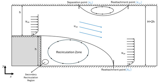
Figure 1.
The geometry of BFS with the recirculation zone, the secondary recirculation region where a second smaller vortex exists and the potential flow where the velocity is equal to .
The novelty of this study arises from the extension of MHD flow over a BFS at various angles of magnetic field and different Stuart numbers. Additionally, the numerical procedure of FVM with the Levenberg–Marquardt algorithm is validated in the MHD and hydrodynamics cases. The results are in excellent agreement with the calculations of the normalized reattachment point (), the length of the upper wall bubble and the velocity profile in distance and . We have developed an advanced numerical algorithm based on Newton–like methods, such as the Levenberg–Marquardt approach for the solution of a strongly nonlinear system of partial differential equations (PDEs). This approach provides robust and reliable results and always converges to the solution. A numerical code was developed in MATLAB (version 2024b, MathWorks, Inc., Natick, MA, USA). So, the literature gap is addressed with this study, presenting robust results on MHD effect on the flow field in different angle configurations, highlighting the pressure field in all the cases studied.
2. Mathematical Formulation
2.1. Magnetic Field Configuration
In this study, a uniform magnetic field is applied to the fluid flow at an angle, . This type of magnetic field is applied to the entire fluid. In mathematical form, the uniform magnetic field is given by the magnetic induction [22],
where and are the magnetic induction components (uniform magnetic field) and is the magnetic field magnitude measured in Tesla (T),
The influence of the magnetic field on fluid flow is maximized when the magnetic field is applied vertically, . The change in angle below results in a minimized effect of the magnetic field, as shown in Figure 2. The numerical results for different angles are presented in a later section.
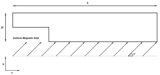
Figure 2.
Backward-facing step for a uniform magnetic field at an angle .
2.2. Dimensional and Non-Dimensional Governing Equations
The governing equations that formulate the flow of an electrically conducting fluid under the influence of an externally applied, uniform magnetic field are the Navier–Stokes along with the Conservation of Mass equations [22],
where and are the dimensional fluid velocity components, is the dimensional fluid pressure. is the fluid density, measured in kilograms per cubic meter (kg/m2) is the fluid viscosity, measured in Pascal seconds (Pa · s). is the electrical conductivity, measured in Siemens per meter (S/m). The induced magnetic field is considered negligible [23].
To obtain the non-dimensional forms of Equations (3)–(5), the following non-dimensional quantities are introduced as follows:
where H is the channel height measured in meters (m), measured in meters per second (m/s). The quantity is the magnetic field magnitude measured in Tesla (T),
The non-dimensional governing equations are written in closed form as follows:
where is the Reynolds number and N is the Stuart number as follows [22]:
2.3. Boundary Conditions
The boundary conditions for the problem under consideration are
The inflow velocity profile is identical to the studies we compare with. The value of average velocity is equal to and is used for the calculation of . At the outlet channel region of BFS, Neumann boundary conditions are applied for the two components of velocity and zero pressure Dirichlet boundary condition is applied. On the walls of the BFS geometry, a no-slip boundary condition is enforced for the fluid velocity. The case of is fundamental and the most studied; therefore, the choice for the expansion rate to compare with as many studies as possible.
The present mathematical formulation is based on the following assumptions: laminar, incompressible and steady state fluid flow while the induced magnetic field is neglected under the low magnetic Reynolds number approximation. The analysis is restricted to two-dimensional fluid flow. The fluid properties are constant and isotropic and thermal effects are ignored. Additionally, electrically insulated walls are assumed so that no current passes through the boundaries.
3. Numerical Methodology
The discretization approach used in the current study is the Finite Volume Method (FVM), a second-order accuracy method, due to the central scheme used to discretize the governing equations [24,25]. This method transforms the system of nonlinear partial differential equations into a nonlinear system of algebraic equations over each finite volume. The computational domain is divided into a finite number of volumes, composed of partitions of the domain. By integrating the governing Equations (8) and (9) over the control volume, the required system is obtained, where in a residual form is provided as follows:
and are the dimensions of the control volume and and N are the East, West, Centroid, South and the North of the control volume.
The numerical solution is obtained by solving Equations (12)–(14) using a Newton-like method [26]. In general, Newton-like methods use the Jacobian matrix, that are calculated as follows:
The functions and are the residual equations obtained by the discretization scheme Equations (12)–(14) and the variables and are the vectors of the unknown parameters of the fluid velocities and pressure. In large-scale problems, such as the one presented in this study, the evaluation of the Jacobian matrix, J, can be computationally expensive [27]. The sparsity of the Jacobian matrix was utilized, saving substantial amount of memory while deceasing the computational time. It has been observed that the number of zero elements increases as the grid becomes finer, implying that the number of elements equal to zero is vastly greater than the non-zero ones [27].
Solving the algebraic system with Newton-like methods provides a different approach compared to other solvers such as SIMPLE-PISO and Stream–Function Vorticity formulation. The proposed method does not use additional equations to simplify the nonlinear system. The coupled system is solved simultaneously at each Newton iteration, while the Jacobian matrix is calculated once per iteration, saving computational time and space. Convergence is obtained when Equations (12)–(14) are as close to zero as possible. A small tolerance value () is defined to stop the solver procedure. If this criterion is satisfied, a vector solution is obtained which contains the resolved unknown parameters and p [26].
The in-house solver developed in this work relies on a finite-volume discretization of the governing fluid flow equations along with MHD terms applied to them, ensuring discrete conservation and consistency, coupled with a nonlinear optimization scheme based on the Levenberg–Marquardt (LM) algorithm. The finite-volume framework is widely used in computational fluid dynamics and provides a robust foundation for stability and accuracy [28,29,30]. The LM algorithm, originally designed for nonlinear least-squares optimization [30], can be regarded as a Newton-like method with trust-region regularization. Compared to iterative solvers, classical Newton or quasi-Newton approaches, LM offers a larger convergence radius, improved stability in ill-conditioned nonlinear systems, and a good balance between robustness and computational efficiency. These features make it particularly suitable for the BFS-MHD configuration considered here, where strong coupling and nonlinear effects often challenge direct solvers.
4. Results and Discussion
In this work, we studied the BFS in the hydrodynamic and magnetohydrodynamic case. The BFS is a valuable test problem for testing new developed codes and the accuracy of new numerical methods. The flow over BFS combines the phenomenon of separation, recirculation region, and the existence of a primary vortex generated in the recirculation zone. In some special cases with certain expansion rates and a specific Reynolds number , a secondary vortex emerges at the low corner of the step. The application of the MHD principles results in the disturbance of fluid flow. The momentum is reduced along the vortex length, and the reattachment point is shifted.
The numerical results presented are obtained through a mesh grid of the size of which results in control volumes providing a higher spatial resolution and ensuring greater accuracy in capturing gradients and flow characteristics. During the study of the BFS flow, a grid independence study has been conducted using progressively finer grids. Maximum differences of up to have been observed for the location of the reattachment point at the bottom wall for numbers in the range of 100 to 800. Thus, the coarser grid was considered sufficiently accurate and was subsequently used to obtain the numerical results.
4.1. Hydrodynamic Case
Backward-facing step flow in the hydrodynamic case is studied for different Reynolds numbers, from 100 to 800 with step 100. The results include the u-velocity component, pressure distribution, skin friction coefficient, and vital values such as these of normalized reattachment point, and normalized length of the bubble in the upper wall, , to evaluate the results with other studies.
The u-velocity can be observed in Figure 3 for four different cases and 800 with maximum inlet-velocity of . In the upstream region of the BFS, the flow is fully developed and remains symmetrical. After the step, separation of flow causes a significant change in the velocity profiles, creating a recirculation zone. The profile in this region shows negative velocities near the wall due to flow reversal. Furthermore, the pressure distribution for the aforementioned cases is presented in Figure 4. As increases, the fluid flow presents more intense recirculation and a longer reattachment length. In consequence, the primary vortex becomes wider. This occurs because the inertia of the flow dominates the viscous forces as increases. A second bubble is emerging in the upper wall at . This is anticipated and validates the results of the developed methodology [5,9].
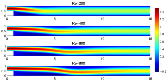
Figure 3.
u-velocity contours for and 800, respectively.
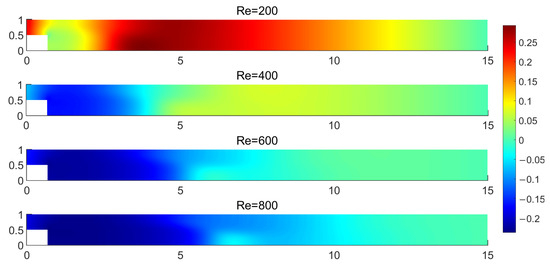
Figure 4.
Pressure distribution contours for and 800, respectively.
The streamlines highlight the presence of the primary vortex defining the recirculation region. The reattachment point is calculated by the stresses on the wall, or the skin friction coefficient, . Mathematically, and are linked by the expression, . Consequently, the reattachment point is defined as the point that and are becoming zero. Similarly, the separation point and the second reattachment point on the upper wall are defined. Table 1 shows the normalized distances of the reattachment and separation points for various . In the last column, the length of the upper-wall bubble is computed to facilitate comparison with other studies.

Table 1.
Normalized reattachment distances of lower wall , upper wall separation point, distance in upper wall , and length of bubble in upper wall, .
The formation and length of the two bubbles have become the most important tests for validation in BFS flows. In Figure 5, the two bubbles for are presented with streamlines. In the pressure distribution, the step in geometry lead to flow separation. The pressure in the region upstream of the step, shows a typical pressure distribution for a channel. After the step, there is a sudden pressure drop due to flow separation, which is recovering progressively as the flow approaches the reattachment point. After this point, the pressure gradually reaches the boundary condition value applied at the end of the geometry.
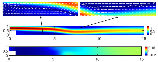
Figure 5.
BFS for u-velocity zoomed with streamlines in the lower bubble (left) and upper bubble (right). Pressure distribution in the second figure. Figures correspond to .
In Figure 6, the skin friction coefficient on both walls is presented, after the step. It can be observed that on lower wall, is equal to zero in one location, at the reattachment point, and on the upper wall is equal to zero in two locations. The first one defines the separation or else detachment point, and the second one defines the reattachment point of the upper bubble, .
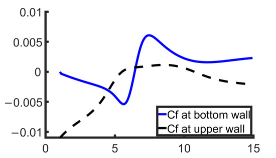
Figure 6.
Skin friction coefficient in both upper (solid) and lower (dashed) wall.
4.2. Validation
Validation of the results is essential for further investigation of the MHD effects in the flow over a BFS. A key indication of the robustness of the findings is the agreement between the reattachment point on the lower wall and the length of the upper wall bubble. The upper bubble exists for greater than 400. Numerous studies have verified as the critical value for the appearance of the upper bubble.
In Table 2, the reattachment point is compared to several other studies that compare the normalized reattachment point and achieve very good agreement for the numerical results in the case of . Additionally, the normalized length of the upper bubble presents very good agreement in comparison with other authors. In these two critical values, the small differences can be explained by the difference in numerical schemes and discretization methods. The comparison of the results with other works is evaluated as very good, considering that most authors use the stream function–vorticity formulation, which differs drastically from this methodology and results in small differences.
Table 2.
Comparison of and values with percentage error.
As Armaly et al. have demonstrated, the experimental studies vary enough from the numerical ones, at the range of due to the three-dimensionality of BFS flow, causing the two-dimensional numerical results to differ moderately from the experimental measurements [5]. As depicted in Figure 7, the experimental measurements of Armaly begin to differ noticeably after , as the numerical results of several studies tend to follow an underestimate of the experimental results for an expansion ratio of . Numerical studies of the most influential works in flow over BFS, are compared with our results and present very good agreement for all ranges of Reynolds numbers from 100 to 800.
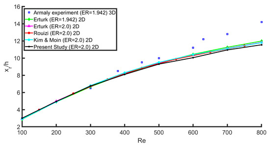
Figure 7.
Comparison of present study normalized reattachment point () with experimental and numerical data [4,5,9,37].
A more detailed quantitative comparison shows that the normalized reattachment length at in the present study () differs by from Rogers & Kwak [31], from Erturk [9], and from Lee & Mateescu [6]. Similarly, the predicted upper-wall bubble length differs by only from Rogers & Kwak [31] and from Lee & Mateescu [6]. These deviations are within the range typically reported for BFS benchmarks and confirm that the present solver reproduces the canonical flow behavior with high accuracy.
It is worth noting that the minor discrepancies observed for > 600 are consistent with previous numerical and experimental findings. In this regime, two-dimensional steady-state models tend to deviate from experiments because the BFS flow becomes strongly three-dimensional and transitional in nature [5,11].
The negligible differences presented in the implemented comparison can be explained in the different discretization scheme, the different solver for the nonlinear system of equations, or in the slightly shorter length section we use compared to other studies. Another crucial aspect is the u-velocity profile. In the present study, the velocity profile at the downstream location of the step at and is compared to the corresponding result of Erturk [9], presenting a perfect fit, as shown in Figure 8.
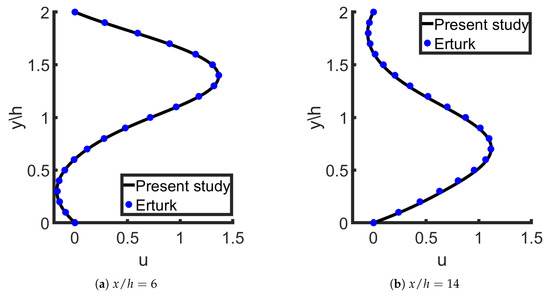
Figure 8.
Validation of horizontal profile in and with a comparison of the present study (black solid line) with Erturk profile (blue dotted line) [9].
Finally, our results are satisfactory as the validation of both lower- and upper-wall bubbles are in acceptable range. This outcome provides a solid foundation for proceeding with the implementation of the fluid flow over BFS adding the MHD effects, presented in the next section.
5. Magnetohydrodynamic Flow Validation
In the present study, a uniform magnetic field is applied in various magnitudes and angles. The hydrodynamic case revealed the creation of vortices and the numerical results were validated with published studies. The application of a uniform magnetic field, due to Lorentz forces, opposes the flow. The application of the uniform magnetic field is examined in two cases, (a) the application of different magnetic field magnitudes, while the magnetic field is vertically applied to the lower wall, (b) the application of a constant magnetic field applied in various angles. A comparison with Abbassi and Nassrallah has a small error of u-velocity distribution at validating the MHD approach.
Figure 9 shows the u-velocity at and inside the channel, respectively. At the first point the velocity presents negative values due to the creation of the vortex, whereas at the second point the velocity is closer to a parabolic profile, indicating that the flow develops. The results are also in good quantitative agreement with those of study [16].
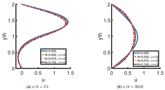
Figure 9.
Validation of horizontal profile in and for various Stuart numbers for .
Figure 10 shows the change in the normalized reattachment point for the hydrodynamic and magnetohydrodynamic case, respectively. Due to the effect of the magnetic field, the reattachment point decreases. It should be noted that the vortices that are present for , in the hydrodynamic case at the upper wall are completely vanished, since does not change sign. The reattachment point in the case of , and is close to that of in the hydrodynamic case, indicating that there is no vortex in the upper wall.
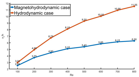
Figure 10.
Comparison of the normalized reattachment points for the Hydrodynamic (orange) and Magnetohydrodynamic (blue) case, respectively, for and .
5.1. Vertically Applied Magnetic Field
The numerical simulations showed that the velocity decreases as the magnetic field magnitude increases. The pressure increases as the magnetic field magnitude is amplified, since the magnetic field opposes the fluid. A visual representation for the pressure increase is shown in Figure 11. As a result of the velocity drop, the length of the vortex is reduced as the magnitude of the magnetic field increases. A visual representation of the reduction in the vortex in each case is shown in Figure 12, as the magnetic field increases.
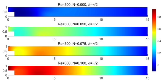
Figure 11.
Pressure contours for , and Stuart number (hydrodynamic case), and , respectively.
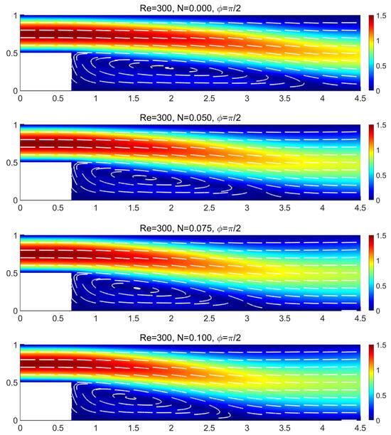
Figure 12.
Creation of vortices for , and Stuart number (hydrodynamic case), and , respectively.
The vertical magnetic field induces a Lorentz force that opposes the fluid motion inside the domain. This generates drag that reduces momentum transfer in the shear layer and as a result, the reattachment point shifts closer to the step. At the same time, because the Lorentz force resists forward acceleration, a stronger adverse pressure gradient develops, which explains the observed pressure increase. The secondary vortex vanishes because the damping effect of the Lorentz force inhibits the backflow and roll-up of the shear layer that would otherwise generate it. The strength of these effects grows with the Stuart number (N), since a stronger magnetic field yields a stronger Lorentz force and therefore greater suppression of vortices and increased drag.
5.2. Magnetic Field Magnitude with Various Angles
In this case, the Stuart number was , whereas the angle was set to and , respectively. The effect of the magnetic field on the pressure is visible at Figure 13. Lateral pressure is observed in all cases, while the pressure values has the maximum effect as the magnetic field angle is .
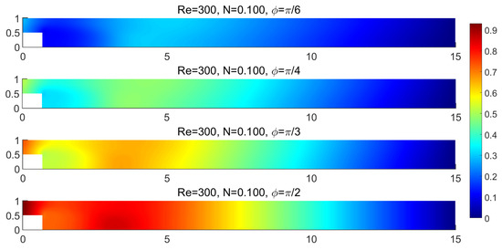
Figure 13.
Pressure contours for , and and , respectively.
The u-velocity is depicted for and , for different angles. It can be seen that in the case of , is closer to the hydrodynamic case compared to the case of where the fluid flow is considerably reduced. The vortex length becomes smaller, as the angle increases, Figure 14.

Figure 14.
Creation of vortices for , and angles and , respectively.
5.3. Limitations and Future Steps
The study of BFS exhibits great interest in three dimensions due to the asymmetries observed in the reattachment points in the z-direction. The numerical procedure used can be extended to the three-dimensional case of BFS to compare with three-dimensional experimental studies. A preliminary study was conducted, and the boundary conditions are identical to the two-dimensional study, expanded in z-direction. The results depicted in Figure 15 show the u-velocity of the fluid. The results were produced by the same numerical algorithmic procedure, described in the present study, expanded in the three-dimensional case for a grid size of .
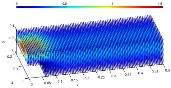
Figure 15.
Scatter plot for the u-velocity component, in the case of the 3D backward-facing step for .
The present work is relevant to diverse applications where sudden expansions and recirculating regions occur under external magnetic fields, such as electromagnetic control in metallurgical processes, liquid-metal cooling in nuclear reactors, plasma propulsion systems, and biomedical flows in arterial expansions. These examples highlight the importance of understanding MHD flow behavior in BFS geometries and motivate the present study.
Changing the attribute of the magnetic field from uniform to non-uniform would provide new insights into its effects in such a problem, since it is expected to locally disturb the vortex generated by the fluid flow and the geometry. Furthermore, an advanced turbulence model, utilizing two-equation models or Large Eddy Simulation, will be pursued to examine the robustness of the algorithm in situations that include extended recirculation regions with strongly nonlinear dynamics.
6. Conclusions
This work studies the accuracy and robustness of a numerical framework for simulating magnetohydrodynamic (MHD) flow over a BFS. The governing equations were discretized using a second-order FVM on a collocated grid and solved directly utilizing a Newton-like algorithm. The solver provides robustness and efficiency with reliable convergence. This approach is preferable to this problem, as intense source terms may result in a lack of convergence in the case of an inappropriate iterative approach. The numerical methodology was validated against a wide range of well-established hydrodynamic benchmarks, including reattachment lengths across several Reynolds numbers. The results showed very good agreement with previous numerical and experimental studies, confirming the accuracy and applicability of the proposed numerical approach.
Beyond the present laminar two-dimensional configuration, the proposed Newton-based finite-volume framework is relative easy extendable to more complex scenarios. In particular, its robustness, due to the LM methology, in handling nonlinear source terms provides a solid foundation for examining turbulence models (RANS, LES, or DNS) and for coupling with multiphase flow formulations where MHD effects are relevant (e.g., liquid–gas metal processing, ferrofluid transport). Moreover, the current formulation can be adapted to three-dimensional geometries, while more complex magnetic fields such as non-uniform or transient can be applied. By applying the energy equation even more advanced problems involving heat transfer can also be studied. The proposed extensions enchance the broader applicability of the methodology proposed and its potential role in advancing MHD simulations in industrial and biomedical contexts.
The presence of the magnetic field reduced the fluid momentum and the reattachment length, and increased pressure due to the Lorentz force. Notably, the field orientation played a critical role, as the strongest effects were observed when the magnetic field was applied vertically , vanishing the secondary vortex that appears in the upper wall at higher Reynolds numbers. By systematically analyzing the impact of both magnetic field strength and direction, this study addresses a gap in the current literature on BFS/MHD flows. Furthermore, a preliminary extension to three-dimensional simulations demonstrates the robustness of the proposed solver and its potential for application in complex flow configurations and future studies involving turbulence or non-uniform magnetic fields.
Author Contributions
Conceptualization, S.K., G.C., M.X. and E.T.; methodology, S.K., G.C., M.X. and E.T.; software, S.K., G.C., M.X. and E.T.; validation, S.K., G.C., M.X. and E.T.; formal analysis, S.K., G.C., M.X. and E.T.; investigation, S.K., G.C., M.X. and E.T.; resources, S.K., G.C., M.X. and E.T.; data curation, S.K., G.C., M.X. and E.T.; writing—original draft preparation, S.K., G.C., M.X. and E.T.; writing—review and editing, S.K., G.C., M.X. and E.T.; visualization, S.K., G.C., M.X. and E.T.; supervision, M.X. and E.T.; project administration, M.X. and E.T.; funding acquisition, M.X. and E.T. All authors have read and agreed to the published version of the manuscript.
Funding
This research was implemented in the framework of the Action “Flagship actions in interdisciplinary scientific fields with a special focus on the productive fabric”, which is implemented through the National Recovery and Resilience Fund Greece 2.0 and funded by the European Union–NextGenerationEU (Project ID: TAEDR-0535983).
Data Availability Statement
The original contributions presented in this study are included in the article. Further inquiries can be directed to the corresponding author.
Conflicts of Interest
The authors declare no conflicts of interest.
Correction Statement
This article has been republished with a minor correction to the Data Availability Statement. This change does not affect the scientific content of the article.
References
- Papanastasiou, T.; Malamataris, N.; Ellwood, K. New outflow boundary condition. Int. J. Numer. Methods Fluids 1992, 14, 587–608. [Google Scholar] [CrossRef]
- Gartling, D.K. A test problem for outflow boundary conditions—Flow over a backward-facing step. Int. J. Numer. Methods Fluids 1990, 11, 953–967. [Google Scholar] [CrossRef]
- Ayyagari, T.; He, Y. Aerodynamic analysis of an active rear split spoiler for improving lateral stability of high-speed vehicles. Int. J. Veh. Syst. Model. Test. 2017, 12, 217. [Google Scholar] [CrossRef]
- Kim, J.; Moin, P. Application of a fractional-step method to incompressible Navier-Stokes equations. J. Comput. Phys. 1985, 59, 308–323. [Google Scholar] [CrossRef]
- Armaly, B.F.; Durst, F.; Pereira, J.C.F.; Schönung, B. Experimental and theoretical investigation of backward-facing step flow. J. Fluid Mech. 1983, 127, 473–496. [Google Scholar] [CrossRef]
- Lee, T.; Mateescu, D. Experimental and Numerical Investigation of 2-D Backward-Facing Step Flow. J. Fluids Struct. 1998, 12, 703–716. [Google Scholar] [CrossRef]
- Chen, L.; Asai, K.; Nonomura, T.; Xi, G.; Liu, T. A review of Backward-Facing Step (BFS) flow mechanisms, heat transfer and control. Therm. Sci. Eng. Prog. 2018, 6, 194–216. [Google Scholar] [CrossRef]
- Valencia, A. Pulsating Flow in a Channel with a Backward-Facing Step. Appl. Mech. Rev. 1997, 50, S232–S236. [Google Scholar] [CrossRef]
- Erturk, E. Numerical solutions of 2-D steady incompressible flow over a backward-facing step, Part I: High Reynolds number solutions. Comput. Fluids 2008, 37, 633–655. [Google Scholar] [CrossRef]
- Thangam, S.; Knight, D.D. Effect of stepheight on the separated flow past a backward facing step. Phys. Fluids A Fluid Dyn. 1989, 1, 604–606. [Google Scholar] [CrossRef]
- Liakos, A.; Malamataris, N.A. Topological study of steady state, three dimensional flow over a backward facing step. Comput. Fluids 2015, 118, 1–18. [Google Scholar] [CrossRef]
- Choi, H.H.; Nguyen, V.T.; Nguyen, J. Numerical Investigation of Backward Facing Step Flow over Various Step Angles. Procedia Eng. 2016, 154, 420–425. [Google Scholar] [CrossRef]
- Tsay, Y.L.; Chang, T.S.; Cheng, J.C. Heat transfer enhancement of backward-facing step flow in a channel by using baffle installation on the channel wall. Acta Mech. 2005, 174, 63–76. [Google Scholar] [CrossRef]
- Demuren, A.O.; Wilson, R.V. Estimating Uncertainty in Computations of Two-Dimensional Separated Flows. J. Fluids Eng. 1994, 116, 216–220. [Google Scholar] [CrossRef]
- Davidson, P. Introduction to Magnetohydrodynamics; Cambridge Texts in Applied Mathematics, Cambridge University Press: Cambridge, UK, 2017. [Google Scholar]
- Gürbüz, M.; Tezer-Sezgin, M. MHD Stokes flow in lid-driven cavity and backward-facing step channel. Eur. J. Comput. Mech. 2015, 24, 279–301. [Google Scholar] [CrossRef]
- Cherkaoui, I.; Bettaibi, S.; Barkaoui, A.; Kuznik, F. Numerical study of pulsatile thermal magnetohydrodynamic blood flow in an artery with aneurysm using lattice Boltzmann method (LBM). Commun. Nonlinear Sci. Numer. Simul. 2023, 123, 107281. [Google Scholar] [CrossRef]
- Tzirtzilakis, E. Biomagnetic fluid flow in a channel with stenosis. Phys. D Nonlinear Phenom. 2008, 237, 66–81. [Google Scholar] [CrossRef]
- Abbassi, H.; Ben Nassrallah, S. MHD flow and heat transfer in a backward-facing step. Int. Commun. Heat Mass Transf. 2007, 34, 231–237. [Google Scholar] [CrossRef]
- Al-Habahbeh, O.; Al-Saqqa, M.; Safi, M.; Khater, T. Review of magnetohydrodynamic pump applications. Alex. Eng. J. 2016, 55, 1347–1358. [Google Scholar] [CrossRef]
- Rashidi, S.; Esfahani, J.A.; Maskaniyan, M. Applications of magnetohydrodynamics in biological systems-a review on the numerical studies. J. Magn. Magn. Mater. 2017, 439, 358–372. [Google Scholar] [CrossRef]
- Raptis, A.; Xenos, M.; Tzirtzilakis, E.; Matsagkas, M. Finite element analysis of magnetohydrodynamic effects on blood flow in an aneurysmal geometry. Phys. Fluids 2014, 26, 101901. [Google Scholar] [CrossRef]
- Rajput, U.; Kumar, S. Rotation and radiation effects on MHD flow past an impulsively started vertical plate with variable temperature. Int. J. Math. Anal. 2011, 5, 1155–1163. [Google Scholar]
- Versteeg, H.K. An Introduction to Computational Fluid Dynamics: The Finite Volume Method, 2nd ed.; Pearson Education Ltd.: Harlow, UK, 2007. [Google Scholar]
- Katsoudas, S.; Malatos, S.; Raptis, A.; Matsagkas, M.; Giannoukas, A.; Xenos, M. Blood Flow Simulation in Bifurcating Arteries: A Multiscale Approach After Fenestrated and Branched Endovascular Aneurysm Repair. Mathematics 2025, 13, 1362. [Google Scholar] [CrossRef]
- Quarteroni, A.; Sacco, R.; Saleri, F. Numerical Mathematics; Springer Science & Business Media: Berlin/Heidelberg, Germany, 2007; Volume 37. [Google Scholar] [CrossRef]
- Davis, T.A.; Rajamanickam, S.; Sid-Lakhdar, W.M. A survey of direct methods for sparse linear systems. Acta Numer. 2016, 25, 383–566. [Google Scholar] [CrossRef]
- Ferziger, J.H.; Períć, M.; Street, R.L. Computational Methods for Fluid Dynamics, 4th ed.; Springer: Cham, Switzerland, 2020. [Google Scholar] [CrossRef]
- Patankar, S.V. Numerical Heat Transfer and Fluid Flow, 1st ed.; CRC Press: Boca Raton, FL, USA, 1980. [Google Scholar] [CrossRef]
- Moré, J.J. The Levenberg–Marquardt algorithm: Implementation and theory. In Lecture Notes in Mathematics; Watson, G.A., Ed.; Springer: Berlin/Heidelberg, Germany, 1978; Volume 630, pp. 105–116. [Google Scholar] [CrossRef]
- Rogers, S.E.; Kwak, D. An upwind differencing scheme for the incompressible navier–strokes equations. Appl. Numer. Math. 1991, 8, 43–64. [Google Scholar] [CrossRef]
- Barton, I.E. The entrance effect of laminar flow over a backward-facing step geometry. Int. J. Numer. Methods Fluids 1997, 25, 633–644. [Google Scholar] [CrossRef]
- Guj, G.; Stella, F. Numerical solutions of high-Re recirculating flows in vorticity-velocity form. Int. J. Numer. Methods Fluids 1988, 8, 405–416. [Google Scholar] [CrossRef]
- Grigoriev, M.M.; Dargush, G.F. A poly-region boundary element method for incompressible viscous fluid flows. Int. J. Numer. Methods Eng. 1999, 46, 1127–1158. [Google Scholar] [CrossRef]
- Keskar, J.; Lyn, D. Computations of a laminar backward-facing step flow at Re = 800 with a spectral domain decomposition method. Int. J. Numer. Methods Fluids 1999, 29, 411–427. [Google Scholar] [CrossRef]
- Gresho, P.M.; Gartling, D.K.; Torczynski, J.R.; Cliffe, K.A.; Winters, K.H.; Garratt, T.J.; Spence, A.; Goodrich, J.W. Is the steady viscous incompressible two-dimensional flow over a backward-facing step at Re = 800 stable? Int. J. Numer. Methods Fluids 1993, 17, 501–541. [Google Scholar] [CrossRef]
- Rouizi, Y.; Favennec, Y.; Ventura, J.; Petit, D. Numerical model reduction of 2D steady incompressible laminar flows: Application on the flow over a backward-facing step. J. Comput. Phys. 2009, 228, 2239–2255. [Google Scholar] [CrossRef]


Disclaimer/Publisher’s Note: The statements, opinions and data contained in all publications are solely those of the individual author(s) and contributor(s) and not of MDPI and/or the editor(s). MDPI and/or the editor(s) disclaim responsibility for any injury to people or property resulting from any ideas, methods, instructions or products referred to in the content. |
© 2025 by the authors. Licensee MDPI, Basel, Switzerland. This article is an open access article distributed under the terms and conditions of the Creative Commons Attribution (CC BY) license (https://creativecommons.org/licenses/by/4.0/).