Abstract
Maritime transportation companies operate in highly volatile environments, where data-driven decision-making is critical to navigating fluctuating freight revenue, fuel and transit costs, and dynamic trade-related policies. This study addresses the liner service network design and container flow management problem, with the objective of maximizing weekly profit, calculated as total freight revenue minus comprehensive operational costs associated with fuel, berthing, transit, and policy-driven extra fees. We formulate a mixed-integer programming (MIP) model for the problem and demonstrate that the constraint matrix associated with vessel leasing is totally unimodular. This property permits the reformulation of the original MIP model into a semi-relaxed MIP model, which maintains optimality while improving computational efficiency. Using shipping data in a realistic liner service network, the proposed model demonstrates its practical applicability in balancing complex trade-offs to optimize profitability. Sensitivity analyses provide actionable insights for data-driven decision-making, including when to expand service networks, discontinue unprofitable routes, and strategically deploy vessel leasing to mitigate rising operational costs and regulatory penalties. This study provides a practical, computationally efficient, and data-driven framework to support liner shipping companies in making robust tactical decisions amid economic and regulatory dynamics.
Keywords:
maritime transportation; fleet deployment model; mixed-integer programming; totally unimodular; data-driven decision-making; realistic shipping data MSC:
90C11
1. Introduction
Maritime transportation is the backbone of global trade, facilitating the movement of a vast majority of the world’s manufactured goods. However, the industry is marked by intense competition and significant operational complexities. Shipping companies must navigate a dynamic environment marked by volatility in freight revenues, fuel prices, demand, and transit costs. Such market fluctuations exacerbate operational challenges, necessitating adaptive strategies to maintain resilience and competitiveness [1]. Variable costs like handling fees and delays further complicate planning, as mismanagement can lead to longer transit times or reduced reliability [2]. In addition, geopolitical and trade policies, such as surcharges imposed on China-constructed (CN-constructed) vessels calling at US ports, add further financial and strategic risks [3]. These fees could significantly increase operational costs, particularly for bulk commodities like agriculture and coal [4]. Shipping companies may need to reconfigure fleets, prioritize leasing non-CN-constructed vessels, or adjust routes to mitigate costs, and the reduced vessel availability could disrupt supply chains [5]. To sustain profitability and competitiveness, liner companies need advanced decision support tools capable of addressing these interconnected issues [6].
Among the various operational challenges, transshipment plays a pivotal role in enhancing cost efficiency through route optimization, enabling the transfer of containers between vessels, allowing shipping companies to serve ports without direct connections and thereby enhancing operational flexibility and efficiency [7]. However, it also introduces significant strategic and logistical complexities. Global trade disruptions, such as the 70% drop in Suez Canal traffic and the 31% increase in Panama Canal voyage distances in 2024, intensify reliance on transshipment hubs, highlighting their critical role in maintaining supply chain efficiency [8]. The selection of optimal transshipment hubs involves balancing geographic advantages, infrastructure capacity, and handling efficiency, all of which significantly impact network performance [9]. Empty container repositioning addresses the structural imbalances in global trade, where import-heavy regions like Europe and North America generate surplus empty containers, while export-heavy regions like Asia face shortages [10]. This operation ensures containers are available where needed, preventing export delays due to container shortages at export-dominant ports and avoiding storage issues from surplus containers at import-dominant ports [11]. Effective empty container repositioning is crucial for maintaining service reliability and supporting sustainability by reducing unnecessary transport and associated emissions [10]. However, it faces significant challenges, as empty containers occupy valuable space that could be used for laden containers, reducing vessel capacity for revenue-generating cargo [12]. Additionally, careful planning of repositioning routes is essential to ensure transportation efficiency and economic viability, as inefficient routing can lead to delays and operational inefficiencies [13]. Failing to prioritize transshipment and empty container repositioning can lead to inefficient routing, reduced service reliability, and diminished competitiveness in the liner shipping landscape, making these operations crucial for maintaining efficient and resilient supply chains.
Advanced optimization models, such as mixed-integer linear programming, are essential for managing transshipment operations, optimizing hub selection, and mitigating uncertainties, all of which are crucial to maintaining competitiveness in a rapidly evolving trade environment [14]. Existing research on liner shipping planning reveals significant gaps. Many studies focus on isolated decisions, such as network design [15], fleet deployment [16,17], or container flow management [18,19]. This fragmented approach often fails to account for the interdependencies among these decisions, potentially leading to suboptimal strategies. Additionally, some models oversimplify operational realities by neglecting the simultaneous consideration of factors like container transshipment, diverse vessel characteristics, and empty container repositioning [18]. There is a critical lack of integrated models that account for trade-offs from policy-driven financial penalties, such as emission control areas [15] or policy-driven surcharges, which are increasingly relevant in today’s trade environment. Moreover, large-scale mixed-integer programming (MIP) models used for integrated planning face computational challenges, limiting their practical application in tactical decision-making [7,14].
To address these gaps, we formulate a liner service network design and container flow management (LSND–CFM) problem under volatile market conditions, including fluctuating freight revenues, operational costs, container transshipment, and dynamic trade policies. The LSND–CFM problem jointly optimizes route selection, vessel leasing and assignment, laden container transportation with transshipment, and empty container repositioning. To aid in integrated decision-making, we develop an MIP model that includes practical constraints like fleet size limits, weekly service frequency, and policy-specific penalty avoidance. Furthermore, we leverage the total unimodularity (TU) property of the leasing constraint matrices to prove that the decision variables related to vessel leasing can be relaxed to be continuous. This allows for the reformulation of the original model into a semi-relaxed MIP (SRMIP) model, which preserves solution optimality while significantly improving computational efficiency. Overall, the proposed SRMIP model provides a reliable and efficient data-driven optimization framework for tactical planning in liner shipping.
The main contributions of this work can be summarized as follows:
- We develop an MIP model that strategically integrates shipping network design and operational planning. The model simultaneously determines route operations, heterogeneous fleet deployment, vessel leasing decisions, and laden/empty container flows, using realistic data to enhance decision-making and operational efficiency.
- We propose a SRMIP Model that leverages the TU property of the vessel leasing constraint matrix. Through a real-world case study, we show that this model achieves identical optimal solutions to the original MIP but with substantially improved computational efficiency. Theoretically, this demonstrates how exploiting TU properties enables partial relaxation of decision variables, contributing to the broader literature on exact optimization.
- We conduct sensitivity analyses on freight revenue, transit cost, fuel price, and policy-driven fees, yielding several managerial insights as follows: (i) high freight revenues justify network expansion and the leasing of additional capacity; (ii) rising transit costs necessitate prioritizing direct routing and discontinuing services heavily dependent on transshipment; (iii) higher fuel prices call for optimizing fleet composition toward more fuel-efficient vessels, even at the expense of some capacity; (iv) policy-driven penalties can be effectively managed with flexible leasing strategies, with a clear threshold between paying fees and vessel substitution; (v) freight revenue remains the dominant driver of profitability, while fuel, transshipment, and extra fees should be controlled through adaptive fleet adjustments and leasing.
The structure of the remaining sections in this paper is as follows. Section 2 offers an extensive review of the literature on liner service network design, including route operations, vessel allocation, cargo management considering transshipment, and the integration of policy dynamics in liner shipping operations. Section 3 introduces the problem, outlines the formulation of the MIP and SRMIP models, and discusses their integral properties. In Section 4, we validate our model based on a real case study and perform sensitivity analyses on critical parameters. Section 5 concludes the paper.
2. Literature Review
This review provides a comprehensive analysis of optimization models and algorithms for LSND–CFM, focusing on route operations, vessel allocation, cargo flow management considering transshipment, and empty container repositioning in liner shipping. It examines the integration of various models and addresses the impact of uncertainties like transport demand fluctuations and fuel price volatility.
2.1. Route Operations and Vessel Allocation
Route operations and vessel allocation are pivotal in liner shipping, determining service reliability and cost efficiency. These decisions involve assigning vessels to routes, optimizing service frequencies, and balancing operational constraints like fuel consumption and vessel capacity.
Brouer et al. [15] propose a benchmark suite for liner shipping network design, introducing an MIP model for route planning and vessel allocation, which highlights the computational complexity of large-scale models and emphasizes the need for efficient algorithms. Wetzel and Tierney [20] propose an MIP model integrating fleet deployment and vessel repositioning. Their model optimizes vessel allocation across a network of routes, using a novel matheuristic algorithm combining branch-and-cut with heuristic search to tackle computational complexity. Hong et al. [21] develop a sample distribution approximation framework to address fleet deployment under random demand. Elmi et al. [22] focus on ship schedule recovery strategies. Their analysis categorizes uncertainties (e.g., port delays, demand fluctuations) and evaluates robust optimization and heuristic methods, highlighting their role in mitigating disruptions. Qu et al. [23] introduce a liner schedule design model under port congestion, employing queuing theory to predict vessel waiting times. Their mixed-integer non-linear programming model minimizes total service costs, incorporating a container handling efficiency selection mechanism. Computational results on benchmark instances show improved schedule reliability by 20% under congested conditions. Koza et al. [24] develop an integrated MIP model for fleet deployment and ship scheduling, optimizing vessel allocation, port call frequencies, and cargo flows. Their column generation-based algorithm reduces operational costs by 8–12% in large-scale networks. Psaraftis and Kontovas [25] analyze speed optimization, formulating an MIP model to balance fuel costs and service reliability. Their model incorporates bunker price volatility and emission constraints, showing a 5–10% reduction in fuel costs while maintaining schedule adherence.
2.2. Cargo Acceptance, Transshipment, and Empty Container Repositioning
Cargo acceptance, container transshipment, and empty container repositioning are essential for maintaining efficient container flows in liner shipping. These processes aim to minimize costs while ensuring timely delivery and optimal resource utilization.
Kuzmicz and Pesch [26] review empty container repositioning, categorizing approaches into network-based, simulation, and optimization models. Their analysis highlights trade imbalances as a key challenge for reducing repositioning costs. Notteboom [18] examines the role of transshipment timing, using a time–cost model to quantify delays’ impact on service reliability. The study shows that optimized transshipment operations reduce delays by 10–20%, enhancing network efficiency. Ross et al. [27] propose an MIP model to address empty container repositioning in a sustainable global supply chain, developing an optimization model to minimize repositioning costs. Shintani et al. [28] propose a two-stage network design model integrating empty container repositioning and cargo flows, solved via a genetic algorithm-based heuristic. Montes-Franco et al. [29] present a hybrid approach combining mathematical programming and heuristic methods to tackle the container loading problem to enhance dynamic stability in liner shipping. Their model optimizes cargo placement to improve vessel stability under varying conditions, achieving a 66.7% average container utilization rate across 23 real-world instances.
2.3. Liner Service Network Design Under Uncertainty
Network design in liner shipping involves determining optimal routes and service configurations to meet customer demands while minimizing costs. Uncertainties, such as demand fluctuations, transit time variability, and fuel price changes, significantly complicate these decisions.
Meng et al. [30] review containership routing and scheduling, analyzing models such as MIP, stochastic programming, and heuristics. Their survey highlights that stochastic models improve cost efficiency by 5–10% under demand uncertainty, stressing the need for robust methods. Christiansen et al. [31] propose a robust optimization model for network design with uncertain transit times, formulated as an MIP with adjustable uncertainty sets. Their branch-and-price algorithm optimizes route configurations, reducing costs by 8% in stochastic scenarios. Huang et al. [32] apply approximate dynamic programming to network design under uncertainty, developing a value function approximation to handle random transit times and demand. Their model improves schedule reliability by 15% in volatile markets. Abioye et al. [33] address ship schedule recovery in emission control areas, developing a robust MIP model that incorporates fuel price volatility and environmental constraints. Computational tests show a 7–10% cost reduction while meeting regulatory requirements. Brouer et al. [15] introduce a benchmark suite for network design, presenting an MIP model with demand variability and port constraints. Their decomposition-based algorithm tackles large-scale instances, reducing computation time by 30%.
2.4. Research Gap
Although the existing literature has seen considerable progress, several important gaps still exist. First, most studies focus on isolated decision areas, such as route operations, fleet deployment, container management, or transshipment strategies without fully addressing their interdependencies. For instance, models for fleet deployment or container repositioning often neglect interactions with cargo transshipment or scheduling, leading to suboptimal solutions that fail to capture the complexity of liner shipping operations. In contrast, this research integrates route selection, vessel allocation, transport demand acceptance, transshipment, and empty container repositioning, offering a holistic optimization framework. Second, while many existing studies consider standard operational costs, they do not adequately model the strategic decisions required to mitigate policy-driven financial penalties, which represent a significant and growing source of financial risk. This research directly addresses this gap by modeling the policy-driven financial penalties as a distinct cost component within the objective function.
To tackle these challenges, we introduce an MIP model for the LSND–CFM problem. This model integrates key decisions such as route operation, fleet management, container transshipment, and the handling of laden and empty container flows. It uniquely considers the impacts of the surcharges on specific vessels by leveraging real-world shipping data. The model also accounts for various practical constraints, such as fleet composition, frequency requirements for route operations, capacity limitations, and empty container balancing constraints. Furthermore, this study conducts extensive sensitivity analyses to evaluate the strategic responsiveness of the optimal solution to shifts in key market parameters. This data-driven approach provides an effective and applicable tool for operational decision-making in liner shipping, enabling companies to adapt to both market dynamics and regulatory changes.
3. Problem Formulation
This section details the research problem. Section 3.1 introduces the operational context and describes the inherent challenges in route selection, vessel assignment, management of laden and empty container flows including transshipment strategies via network paths, and transport demand acceptance. Section 3.2 presents the formulation of an MIP model designed to address these integrated planning decisions. Section 3.3 provides a comprehensive description of the model analysis.
3.1. Problem Description
Shipping companies are continually striving to enhance profitability, expand their service networks, and use their fleet efficiently. Achieving these goals requires making numerous critical decisions, such as determining the operated routes, selecting the most suitable vessels for each route, and deciding the optimal amount of cargo to carry for customers. This decision-making process is further complicated by factors such as volatile fuel prices, fluctuating vessel lease costs, and evolving government regulations.
For a shipping company, several planning areas are closely interconnected and critically important. First, the company selects a set of routes to operate from a range of possible options. Second, it assigns an appropriate number and categories of vessels to each operated route. Third, the company decides how much cargo to accept from customers for each origin-destination (OD) pair. In addition, decisions are made regarding whether cargo should be transshipped, where transshipment should occur if necessary, and how to reposition empty containers throughout the shipping network. Poor coordination among these decisions can lead to significant issues. The company may be forced to reject profitable shipments, and vessels might operate with excessive unused capacity. Careful route selection is therefore essential, taking into account both transportation demand and the operational costs, including fuel cost, berthing cost, transshipment cost, and other surcharges. Additionally, finding the right balance between deploying the company’s owned vessels and leasing vessels strategically, as well as carefully routing both laden and empty containers, is essential to maintain a competitive and financially robust shipping network.
A significant new challenge has arisen with the introduction of proposed port fees for CN-constructed vessels at US ports. These fees specifically target larger CN-constructed vessels, while vessels from other countries or smaller CN-constructed vessels are exempt [3]. For carriers operating a diverse fleet, this means that deploying large-tonnage vessels built in China on certain routes involving US ports can incur avoidable extra charges. As a result, these policy changes have introduced new financial considerations into network and fleet planning. In order to prevent a significant loss of profits, shipping companies must adopt clear and effective strategies that systematically account for such regulatory developments and their impact on operational choices.
We explore the LSND–CFM problem within the framework of a liner shipping network that offers consistent container services on a number of routes. We denote all ports in the framework by , with serving as the index. Transportation demands are specified as OD pairs, with the set containing all such pairs , where and represent departure and arrival ports, respectively. All candidate routes are represented by the set , with serving as the index. Each route is a fixed, cyclic itinerary, structured as a sequential series of legs (indexed by ), wherein each leg denotes the segment of the journey between two consecutive ports of call. Each route operates with a fixed weekly departure frequency. To maintain this schedule, the operator must allocate a sufficient number of vessels, with the required count determined by the route’s round-trip duration. Thus, the total number of vessels needed for route , denoted by , corresponds exactly to the route’s round-trip time in weeks.
One of the central challenges in this planning problem is to determine the specific routing of containers from their origin ports to their corresponding destinations. To address this, a path is defined as a specific sequence of maritime transport legs connecting an origin port to a destination port. This path can represent either direct sailing on a single route or a more complex itinerary that involves transshipment at one or more intermediate ports, where containers are transferred from one vessel to another via ports that are shared between different routes. Each path is composed of a sequence of legs, which represents the set of all legs between consecutive ports of call on the path. If path involves no transshipment, all legs used in the path are from a single route; otherwise, all legs used in the path are from multiple routes. The set of paths that use leg is denoted by . For each port pair , we denote the set of all feasible paths from to by .
Define (indexed by ) as the set of all container types considered. Specifically, this study focuses on two primary container types: dry containers and reefer containers. The weekly laden container transport demand in type for each OD port pair is denoted by , and the corresponding revenue earned per container transported is denoted by . For each container type , the total volume of accepted demand for each port pair cannot exceed , and the liner shipping company has the option to reject some of the demand if fully accepting it would result in unprofitable operations.
We denote all vessel categories by (indexed by ), with CN-constructed vessels forming the subset . One vessel of category can carry twenty-foot equivalent units (TEUs). The company maintains a fleet consisting of vessels for each category . The company can strategically lease in or lease out vessels across all categories, acquiring a vessel at a weekly cost of for inbound leases and earning income at a weekly price of for outbound leases. This adaptive strategy enables the firm to flexibly adjust its operational fleet: it scales up capacity by leasing in vessels during peak demand and obtains additional income by leasing out when surplus tonnage exists. Operating a vessel of category on route for one cyclic trip incurs several expenses: fuel costs , berthing costs , the transit cost, and additional charges that apply specifically to CN-constructed vessels serving US ports (). Thus, for each route , the weekly costs generated by vessel sailing on that route are expressed as for fuel cost, for berthing cost, and for the extra fee applied to CN-constructed vessels reaching US ports. The transit cost per TEU for laden containers in type on path , denoted by , is calculated as the number of transshipments incurred on path , denoted by , multiplied by the unit transshipment cost per TEU for the type’s laden containers , i.e., . For empty containers on path , the transit cost per TEU, denoted by , follows as analogous calculation: , where indicates the unit transshipment cost per TEU for empty containers in type .
The goal of this study is to maximize the weekly profit, which is calculated by taking the total revenue from accepted containerized transport demand, subtracting the total transportation costs, adding the revenue from leasing out idle vessels, and then subtracting the cost of leasing in vessels. Several key decisions are involved in this process. First, the selection of these paths dictate which candidate routes are operated, which is represented by the binary variable . This variable is assigned a value of 1 if route is chosen to be operated; otherwise, it is assigned a value of 0, indicating that the route is not in service. Second, the fleet composition on each operated route is captured by the integer decision variable , which specifies the total quantity of vessels belonging to category that are allocated to serve route . The integer decision variables and respectively indicate the quantity of vessels of category that are leased in and leased out. For each port pair and each path , the weekly transportation volumes of laden and empty containers in type are each defined by continuous decision variables and , which specifies the amount of accepted laden container transport demand and empty containers (in TEUs) in type allocated to path , respectively.
3.2. Model Formulation
This section introduces an MIP model based on the problem setting described above. The model provides a unified framework for optimizing the interconnected strategic decisions inherent in managing a container liner shipping service. The core of the model addresses two primary domains of decision-making. First, it determines the optimal network design and fleet strategy. This includes selecting which routes will be operational, assigning specific vessel types and quantities to those routes, and managing the fleet size through chartering activities. Second, it manages container flows for both dry containers and reefer containers, determining the volume of laden container demand to accept for transport between various port pairs while also deciding the repositioning paths for empty containers. All these decisions are optimized to maximize total weekly profit, with the model balancing this objective against a set of operational constraints. These constraints reflect practical limits on the number of vessels assigned, the availability of serviceable vessels and restrictions on vessel leasing out, caps on transport volumes, constraints on transport capacity, and requirements for balancing empty containers at ports. The main notations used in this study are summarized in Table 1.

Table 1.
Notations used in model formulation.
The MIP model is formulated to optimize vessel routing, leasing decisions, transport demand acceptance, transshipment strategy, and empty container reposition, which is structured as follows:
The objective Function (1) is designed to maximize the total weekly profit, which is composed of four main components: the revenue obtained from the transportation demand that is accepted, the costs related to vessel routing and cargo allocation (including fuel costs, berthing costs, transit costs, and extra fees), the costs associated with leasing in vessels from external providers, and the income earned from leasing out any surplus vessels owned. Constraint (2) ensures service integrity by mandating that the number of vessels assigned to any given operated route must precisely match the quantity needed to sustain its scheduled weekly sailing frequency. Fleet management is governed by two related conditions: Constraint (3) caps the total deployment of any single vessel category within the available fleet size, which incorporates both leased-in and leased-out vessels, while Constraint (4) further restricts the number of leased-out vessels to no more than the original owned fleet of the company. On the cargo side, Constraint (5) aligns transport activities with market conditions, stipulating that the total volume of laden containers moved between any port pair for a specific container type cannot surpass the total market demand. Constraints (6) manage transport capacity: for each distinct maritime leg that forms part of any candidate route, the total combined volume of both laden and empty containers in all types transported on all paths that specifically use this leg must not exceed the transport capacity of the particular route to which this leg belongs. Constraints (7) ensure that for each port in the network and each container type, the total quantity of containers in type dispatched from that port to all other ports must equal the total quantity of containers in the same type received at that port from all other ports. Constraints (8)–(11) are the domains of the decision variables.
Figure 1 illustrates the decision-making flow of our proposed model.
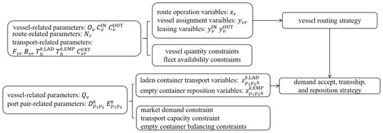
Figure 1.
Decision flow of the MIP model for LSND–CFM problem.
3.3. Model Integrality Properties
This section outlines several theoretical properties associated with the MIP model discussed in Section 3.2.
3.3.1. Integrality Necessity of Binary and Integer Variables
To improve the efficiency of solving the MIP model, we first analyze whether relaxing the binary variables and integer variables can be relaxed. Through a detailed investigation, we establish Lemmas 1 and 2.
Lemma 1.
Relaxing the binary variables to continuous variables results in non-integer solutions, which compromise practical feasibility and violate the problem’s real-world constraints.
Proof.
Consider a counterexample where a single candidate route serves one port pair . Since only one route is considered, no transshipment occurs, and the route can only form a single path . The route needs two vessels for operation, i.e., . The transport demand for this port pair consists of 2000 TEUs dry containers and no reefer container needs to be transported, i.e., TEUs, . The revenue earned per laden dry container transported for is 700 USD/TEU, i.e., USD/TEU. The company owns two identical vessels of category (), each with a transport capacity of 4000 TEUs, i.e., , TEUs. The weekly lease-in cost for one vessel of this category is 0.3 million USD, and the weekly lease-out revenue is 0.2 million USD, i.e., million USD, million USD. Assume the route excludes a US port, then the operational cost for route per vessel consists of the following components: the fuel cost 3 million USD, the berthing cost million USD, and the extra fee of .
Given the instance parameters outlined above, we compare the solutions obtained when the variables are restricted to binary versus when they are relaxed to continuous. For the original MIP model, two possible solutions exist: (i) operating no route, i.e., . This solution is feasible, and the company can lease out all two vessels to earn revenue. The objective value in this case is million USD. (ii) operating route , i.e., . In this case, the shipping company assigns all two owned vessels on the route, i.e., , and no leasing activity occurs, i.e., . Given that the demand is 2000 TEUs and each vessel has a capacity of 4000 TEUs, the demand is completely fulfilled, and the generated empty containers can be repositioned from to through the circular path , i.e., TEUs, and thus constraints (6) and (7) can be satisfied. Therefore, the weekly profit in this scenario can be calculated as follows:
We can conclude that the decision (ii) is optimal. However, if we relax the integer variables to continuous ones, will also be feasible, as the number of required vessels becomes . The company can deploy one owned vessel to route , i.e., , and lease out the remaining idle vessel, i.e., . Since the vessel’s capacity is 4000 TEUs and the weekly transport demand is 2000 TEUs, . Therefore, both the laden container transport demand and the empty container repositioning demand can be fully satisfied through path , i.e., TEUs; thus, constraints (6) and (7) can be satisfied. Then, the objective function value can be calculated as follows:
This relaxed linear programming (LP) solution yields larger objective value compared to that with the integer solution within the relaxation framework. Critically, is practically invalid as we cannot operate a route by half. Therefore, the LP relaxation of inherently results in non-integer solutions, which conflicts with the real-world integer operation requirement, proving cannot be freely relaxed. □
Lemma 2.
Relaxing the binary variables to continuous variables results in non-integer solutions, which compromise practical feasibility and violate the problem’s real-world constraints.
Proof.
Consider a scenario with one candidate route serves one port pair . Since only one route is considered, no transshipment occurs, and the route can only form a single path . The demand of the port pair is entirely for dry containers, with TEUs. The unit freight revenue is USD/TEU. Assume that there are two vessel categories and . The company owns two 4000-TEU vessels of category and one 8000-TEU vessel of category , i.e., , , TEUs, TEUs. The weekly lease-in cost for one vessel of category and is set as 0.3 million USD and 0.5 million USD, respectively, i.e., million USD, million USD. The weekly lease-out revenue for one vessel of category and is set as 0.1 million USD and 0.3 million USD, respectively, i.e., million USD, million USD. Assume the route excludes a US port, then the operational cost for route per vessel of category consists of the following components: the fuel cost 3 million USD, the berthing cost million USD, and the extra fee of . The operational cost for route per vessel of category consists of the following components: the fuel cost 7 million USD, the berthing cost million USD, and the extra fee of .
For the instance stated above, we compare the solutions obtained when the variables are restricted to integers and relaxed to continuous ones, respectively. For the original MIP model, two possible solutions exist: (i) operating no route, i.e., . This solution is feasible, and the company can lease out all three vessels to earn revenue. The objective value in this case is million USD. (ii) operating route , i.e., . In this case, the solution that maximizes the objective function is as follows: The shipping company leases out one vessel of category and assigns the remaining two vessels on the route, i.e., , , . Since , both the laden container transport demand and the empty container repositioning demand can be fully satisfied through path , i.e., TEUs; thus, constraints (6) and (7) can be satisfied. Then, the objective function value can be calculated as follows:
We can conclude that decision (ii) is optimal. However, if we relax the integer variables and to continuous ones, , will also be feasible. In this case, no leasing activity occurs. Since , both the laden container transport demand and the empty container repositioning demand can be fully satisfied through path , i.e., TEUs; thus, constraints (6) and (7) can be satisfied. Then, the objective function value can be calculated as follows:
This relaxed LP solution yields larger objective value compared to that with the integer solution within the relaxation framework. Critically, , are practically invalid as vessels cannot be assigned by half. Therefore, the LP relaxation of inherently results in non-integer solutions, which conflicts with the real-world integer operation requirement, proving cannot be freely relaxed. □
3.3.2. Totally Unimodular Property of the Coefficient Matrix of Variables and
To enhance the computational tractability of the large-scale optimization model presented, this section investigates a method for relaxing its integer variable constraints. This approach is contingent upon ensuring that the relaxation does not compromise the optimality or precision of the final solution. The core of our analysis involves a rigorous examination of the mathematical structure of the model’s constraint matrix. By focusing on the properties of the variables and , we aim to identify the specific conditions under which these variables can be treated as continuous, thereby improving computational performance while maintaining solution integrity.
Our analysis is founded upon the principle of TU, a cornerstone concept in the fields of LP and combinatorial optimization. Formally, a matrix is considered totally unimodular if the determinant of each of its square submatrices is exclusively –1, 0, or 1 [34]. A direct and powerful implication of this property is that for any LP problem where the coefficient matrix is TU and the right-hand-side vector is composed of integers, all basic feasible solutions are inherently integer-valued.
The TU property provides a powerful way for simplifying Integer Linear Programming (ILP) problems. When a problem’s constraint matrix is TU, its integer requirements can be safely removed, transforming the model into a standard LP without sacrificing the integer nature of the optimal solution. The computational benefit of this transformation is significant. While general ILP problems are NP-hard and often require extensive computational resources, LP problems can be solved efficiently with polynomial-time algorithms. Consequently, models in application areas like network flow, resource allocation, and scheduling that feature inherently TU matrices—such as the incidence matrices of bipartite graphs—are considerably more straightforward to solve.
The TU property is crucial for solving Integer Linear Programming (ILP) problems. It allows the relaxation of integer constraints on variables, transforming the problem into a standard LP without losing the integer optimality of the solution. The computational advantage of this transformation is substantial: LP problems can be solved by algorithms with polynomial-time complexity, whereas ILP problems are generally NP-hard and far more time-consuming to solve. As a result, in areas like network flow, scheduling, and resource allocation, models in application areas such as production planning, transportation routing, and workforce assignment are far easier to solve.
The relationship concerning the coefficient matrix of variables and is formalized in the theorem below.
Lemma 3.
The integer variables and can be relaxed to continuous ones as their coefficient matrices are TU for each .
Proof.
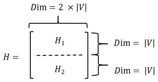
For ease of explanation, we first examine the coefficient matrix corresponding to the variables , denoted as . This matrix is composed of two submatrices:
Let represent the coefficient matrix of the variables , consisting of related to constraints (3) and related to constraints (4). The structure of is shown in Figure 2.
Figure 2.
The structure of the coefficient matrix of the variables .
To prove that matrix is TU, we rely on a widely accepted sufficient condition from [34]. The condition holds if the rows of can be split into two separate groups that satisfy four specific criteria: (i) all entries of belong to ; (ii) no column can have more than two non-zero entries; (iii) if a column has two entries of the same sign, their corresponding rows must belong to different partitions; and (iv) if a column contains two non-zero entries of different signs, their corresponding rows must belong to the same partition.
We apply these criteria to matrix by naturally partitioning its rows into two sets: and . By inspecting constraints (3) and (4), it is evident that in submatrices and , each column contains at most one 1, respectively. This implies that there are no more than two non-zero entries per column in the matrix , and all coefficients belong to , satisfying (i) and (ii). Therefore, we can divide all rows of into a set and that of into another, then the criteria (iii) and (iv) are also satisfied. Thus, we conclude that matrix is TU.
The coefficient matrix associated with the variables is linked solely to constraints (3), and each of its columns contain at most a single entry of , satisfying conditions (i) and (ii). Additionally, since no column has more than one non-zero entry, the criteria (iii) and (iv), which involve pairs of entries with either the same or different signs, do not require further consideration. Consequently, the coefficient matrix corresponding to is TU. Thus, we conclude that the coefficient matrices for both variables and are TU. □
The main advantage of the TU property is its ability to relax integer variables into continuous ones without affecting the integer nature of the optimal solutions, thereby reducing the computational time of the MIP model. More specifically, given any fixed integer variables and integer parameters the right-hand side of constraints (3) and (4) are always integers. As the coefficient matrices of and are TU, these integer variables can be relaxed to continuous ones.
3.3.3. Model Transformation via Variable Relaxation
Based on Lemmas 1–3, we establish Theorem 1 as the main theorem, which formally demonstrates that the original MIP model can be equivalently solved as a more computationally tractable, semi-relaxed formulation. This theorem provides the theoretical foundation for accelerating the model’s computation without sacrificing the optimality and integrality of the final solution.
Theorem 1.
The original MIP model can be transformed into a SRMIP model by relaxing the integer variables for leasing in and leasing out to be continuous.
In the original MIP model, the binary variables for route operation and the integer variables for vessel assignment cannot be relaxed, as this would lead to impractical fractional operations. Conversely, the integer variables related to ship leasing and can be relaxed to be continuous variables because the coefficient matrices of these variables are TU. Therefore, the original MIP model can be transformed into a SRMIP by relaxing this specific subset of decision variables, which enhances computational efficiency without affecting the final optimal solution. Therefore, the SRMIP model is derived from the original MIP model by relaxing the integer constraints (10) to continuous, non-negative variables as follows: .
Moreover, the feasibility of relaxing the variables related to route operation, vessel assignment, and leasing variables is determined by the structural formulation of the model. In particular, the TU property is intrinsic to the leasing constraints and remains valid unless the constraints are significantly altered (e.g., through the introduction of chance constraints or other non-linearities). As a result, the SRMIP model consistently preserves computational efficiency without compromising the optimality or integrality of the final solution, provided the structure of the problem remains consistent with the TU property.
4. Experiments
To assess the effectiveness of the proposed model, a set of computational experiments were conducted. The experiments were executed on a desktop computer equipped with a 13th Gen Intel Core i7 CPU and 32 GB of RAM, utilizing Gurobi Optimizer 10.0.1 through the Python 3.11.5 API. The experimental procedure began with obtaining baseline results using the initial parameter settings, followed by an extensive sensitivity analysis to evaluate the influence of these parameters.
4.1. Experiment Settings
Taking the current liner shipping network as an illustrative example, we select 10 candidate routes and eight vessel categories categorized by size (in TEUs) and country of construction. The parameters settings are given as follows:
Route and port pairs. We consider 10 candidate routes, with their ports of call and the required number of vessels , to ensure a weekly departure frequency derived from [35,36,37,38,39,40]. The routes and their corresponding vessel requirements, along with the specific routes available for direct transfer from each candidate route, are summarized in Table 2. Transshipment is facilitated at any port shared by two or more active routes, enabling container transfers between services. For instance, route can perform direct transfers to routes 3–7, 9, and 10, as it shares one or more ports with them. At these common ports, containers from a vessel on route can be moved onto a vessel serving a connecting route to proceed with their journey.
Table 2.
The parameters for the 10 candidate routes.
We select a set of port pairs and estimate each pairs’ weekly transport demand for dry containers and reefer containers . To keep these estimations in line with real-world market dynamics, we perform rigorous calibration using aggregated containerized cargo flow data and global shipping trend analyses from [41,42,43], ensuring demand sizes and their distribution accurately mirror real trade patterns. The specific settings are summarized in Table 3. By combining these OD port pairs with the route network information in Table 2, we can generate the set of all feasible transport paths for each port pair. These paths may consist of direct sailing on a single route or a multi-route journey involving transshipment.
Table 3.
The weekly transport demands of the port pairs.
Fleet composition and leasing costs. At the core of our experimental setup is a heterogeneous fleet designed to reflect real-world asset management. We define eight vessel categories, which are distinguished by four distinct vessel capacities (3000-TEU, 8000-TEU, 15,000-TEU, and 24,000-TEU) and two construction origin (CN and non-CN). The initial owned fleet composition is directly informed by the deployment data of China COSCO Shipping Corporation Limited across its primary trade lanes [44,45]. In light of the reports suggesting that almost 60% of the vessels owned by China COSCO Shipping Corporation Limited were constructed in China [46], the initial owned fleet is specified as follows: There are a total of 42 CN-constructed vessels, specifically including 5 vessels of 3000 TEUs, 7 vessels of 8000 TEUs, 15 vessels of 15,000 TEUs, and 15 vessels of 24,000 TEUs. The fleet also comprises 28 non-CN-constructed vessels, which consist of 5 vessels of 3000 TEUs, 5 vessels of 8000 TEUs, 10 vessels of 15,000 TEUs, and 8 vessels of 24,000 TEUs. The weekly lease-in prices are set as follows: 0.2 million USD for a 3000-TEU vessel, 0.4 million USD for an 8000-TEU vessel, 0.7 million USD for a 15,000-TEU vessel, and 1.0 million USD for a 24,000-TEU vessel. The weekly revenues generated from leasing these vessels out are set at 80% of the respective lease-in prices, i.e., . Detailed parameters for these eight categories of vessels are presented in Table 4.
Table 4.
The parameters of vessels.
Parameters of freight revenues and transportation costs. The involved ports are classified into three geographic regions: East Asia and Southeast Asia, Western Europe, and North America. Drawing from [47,48,49], we set the freight revenue per transported TEU for both dry laden containers () and reefer laden containers () for each port pair, as detailed in Table 5.
Table 5.
Freight revenue per TEU parameters of port pairs.
Vessel propulsion was assumed to be powered exclusively by very low sulfur fuel oil. Daily fuel consumption for a vessel of category on route at speed is modeled using the formulation from [50]:
where the parameters and correspond to vessel categories. For instance, a vessel on a trans-Atlantic route faces different average sea states and weather conditions than one on an Asia–Europe service, which directly impacts its required engine power and fuel consumption. The fuel cost parameters for vessels with different capacities are presented in Table 6, with the values of and derived from [50].
Table 6.
The fuel cost parameters for vessels of different capacities.
A standardized sailing speed of 20 knots is applied universally. Referring to [51], the unit fuel price (denoted by ) is set at 563.5 USD/ton. Since the round-trip duration (denoted by , in weeks) is equivalent to the required number of vessels , the total fuel expenditure for a vessel of category to complete a round trip on route is computed as . Berthing costs are differentiated by vessel capacity, with each port call costing 0.1 million USD for a 3000-TEU vessel, 0.22 million USD for an 8000-TEU vessel, 0.4 million USD for a 15,000-TEU ship, and 0.6 million USD for a 24,000-TEU vessel. The total berthing expense per round trip on route is thus a product of this per-call cost (denoted by ) and the number of port visits on that route (denoted by ), i.e., . The transshipment costs are set based on [52], with the cost for laden containers at USD 61 per TEU, while for empty containers it is USD 30 per TEU, i.e., USD/TEU, USD/TEU. Then the transit cost per TEU for on path is calculated as follows: , , where denotes the number of transshipments incurred on path . For a path that consists of a single route, the transit cost is 0.
The policy regarding extra fees for CN-constructed vessels calling at US ports is modeled based on [3], where the additional fee per TEU, denoted as , is set at 120 USD/TEU for CN-constructed vessels above 4000 TEUs capacity per rotation. Vessels below 4000 TEUs and those built in other countries are exempt from this fee when calling at US ports.
Algorithm 1 provides a step-by-step pseudo-code of the optimization framework.
| Algorithm 1 Optimization framework for LSND–CFM problem |
| Input: container types (dry, reefer); vessel categories (capacity, owned quantity, leasing costs); candidate routes (legs, weekly frequency); port pair demands and revenues (by container type); transportation cost/penalty parameters. Output: operated routes; fleet assignment per route; lease-in and lease-out strategy; laden and empty flows on paths; weekly profit.
|
The computational complexity of the proposed algorithm can be assessed step by step. Path generation is the most demanding component, as the number of feasible paths for each port pair with transshipments may increase exponentially with network size. In contrast, the remaining steps scale polynomially. Vessel assignments grow linearly with the number of vessel types and candidate routes, demand satisfaction is linear in the number of port pairs and container categories, route capacity enforcement is linear in the number of routes and vessel categories, and empty container balancing is quadratic in the number of ports. Overall, except for the exponential path generation step, all other procedures are of polynomial complexity and remain computationally tractable for the problem sizes considered.
With the initial parameters set, we first generated a baseline solution. Then we performed sensitivity analyses to explore how the outcomes change as these parameters vary.
4.2. Basic Results
This section provides a comprehensive overview of the basic results obtained from the proposed MIP model, including vessel leasing strategy, vessel routing strategy, decisions on freight demand volume, empty container repositioning, the transit volumes, and an analysis of the profit and cost components in the objective function.
4.2.1. Vessel Leasing Strategy
In this section, we present the results of the MIP model. The vessel leasing strategy results are detailed in Table 7. Notably, two vessels of are leased in, while two vessels of are leased out. This indicates a strategic decision is implemented to avoid the extra fees applied to CN-constructed vessels above 4000 TEUs when calling at US ports, which helps the company effectively mitigate these surcharges while optimizing fleet composition and ensuring operational cost efficiency.
Table 7.
Lease-in and lease-out quantities for the eight vessel categories.
4.2.2. Route Operation and Vessel Assignment Strategy
The results related to the route operation and vessel assignment strategy are presented in Table 8.
Table 8.
The routes selected for operation and the assigned vessels.
The results in Table 8 indicate that on the routes which include US ports, only vessels that do not incur extra fees are assigned, including CN-constructed vessels below 4000 TEUs and vessels built in other countries (, –). This strategy effectively avoids the extra fees imposed on larger CN-constructed vessels when calling at US ports.
4.2.3. Transport Demand Acceptance and Empty Container Reposition
The optimization addresses two interconnected objectives: deciding the accepted volume of profitable laden transport demand and determining the necessary volume of empty containers to reposition to correct equipment imbalances. Table 9 summarizes the aggregate weekly volumes for these two critical flows, broken down by dry and reefer container types.
Table 9.
Number of accepted laden containers and repositioned empty containers.
It is observed that the number of accepted laden dry containers is significantly higher, with a total of 410,920 TEUs, compared to 60,320 TEUs for laden reefer containers. This reflects the larger demand for dry container transport in the network. Additionally, 176,570 TEUs of empty dry containers being repositioned and 26,690 TEUs of empty reefer containers repositioned. Efficient repositioning strategies are crucial to ensure that empty containers are repositioned to locations where they are required, helping to maintain service reliability and optimize operational costs.
4.2.4. Port Transshipment Volume Analysis
To analyze the transshipment volume across key ports, we present the top ports with the highest transit volumes in Table 10, which lists the transit volumes (in TEUs) for the top ten ports involved in transshipment along the operated routes.
Table 10.
Top 10 ports by transit volume.
Among the top ten ports, Shanghai leads with the highest transit volume of 34,919 TEUs, while Vancouver registers the lowest at 14,412 TEUs. The total transit volume for the top ten ports combined is 226,854 TEUs. This represents a significant portion of the overall transit volume, which amounts to 426,500 TEUs. Consequently, the top ten ports account for 53.2% of the total transit volume, underscoring their pivotal role in the container transshipment network.
4.2.5. Profit and Cost Analysis
Table 11 leverages the MIP model’s output to provide a full account of total revenue and cost. Figure 3 illustrates a pie chart that visually displays the proportion of each cost component within the total cost structure.
Table 11.
The value and proportion of each component of the objective function.
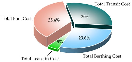
Figure 3.
Composition of total weekly costs in the optimal solution.
The optimal solution achieves a total weekly profit of 440.57 million USD, generated from a total freight revenue of 525.70 million USD. An analysis of the cost components reveals that the total fuel cost is the most significant expenditure at 30.71 million USD. This is followed closely by the total transit cost at 26.02 million USD and the total berthing cost at 25.70 million USD, which constitute comparable shares of the overall expenses. Leasing activities result in a net cost, with 4.30 million USD for leasing in vessels, partially offset by 1.60 million USD in revenue from leasing out surplus vessels. Notably, the total extra penalty cost is zero, which demonstrates the model’s effectiveness in optimizing fleet deployment to completely avoid the surcharges on CN-constructed vessels above 4000 TEUs when calling at US ports, thereby validating its ability to mitigate policy-driven financial risks and enhance the overall profitability of the network.
4.2.6. Comparative Analysis with ALNS
ALNS Framework. To provide a representative metaheuristic baseline, we implement an Adaptive Large Neighborhood Search (ALNS) algorithm. The ALNS approach iteratively destroys and repairs parts of the current solution, thereby exploring a wide neighborhood of the solution space while adaptively learning which operators are most effective. In our context, a solution is represented by the set of operated routes, the assignment of vessels to routes, and the corresponding laden and empty flows.
Destroy and Repair Operators. The destroy phase removes selected components from the current solution to diversify the search. Specifically, we consider three destroy operators: (i) removing a subset of operated routes; (ii) releasing a portion of vessel assignments; and (iii) eliminating selected transshipment flows. The repair phase then reconstructs the solution using heuristic rules: (i) re-inserting candidate routes according to their profitability; (ii) reallocating vessels while accounting for capacity limits and leasing costs; and (iii) reconstructing container flows by shortest path and cost–benefit heuristics.
Acceptance Criterion and Adaptivity. To balance intensification and diversification, the acceptance of new solutions follows a simulated annealing mechanism, where inferior solutions may occasionally be accepted to escape local optima. The algorithm adaptively updates the selection probabilities of destroy and repair operators based on their historical contribution to improving solution quality, thereby ensuring that effective operators are favored in subsequent iterations.
After establishing the ALNS framework, we assess its effectiveness by comparing it with the original MIP formulation and the proposed SRMIP model. This comparison highlights both efficiency and solution quality. Table 12 reports the results in terms of the objective function and CPU time.
Table 12.
Comparison of MIP, SRMIP, and ALNS results.
The results show that both MIP and SRMIP models achieve the same optimal objective value of 440.57 million USD, while ALNS attains a slightly lower optimal weekly profit of 430.88 million USD. This corresponds to a performance gap of approximately 2.2% between ALNS and the optimal solution. In terms of computational time, SRMIP significantly outperforms the original MIP, reducing CPU time by about 67% (from 14.3 s to 4.7 s). Compared with ALNS, SRMIP requires slightly more time but guarantees global optimality, while ALNS sacrifices a small amount of accuracy to achieve the fastest runtime. These results confirm that SRMIP provides a reasonable balance between computational efficiency and solution quality.
4.3. Sensitivity Analysis
The sensitivity analysis is designed to reveal how the model’s outputs respond to fluctuations in key input parameters, such as the unit freight revenue percentage, the unit transit cost percentage, the unit fuel price (USD/ton), and the unit extra fee (USD/TEU) for CN-constructed vessels above 4000 TEUs when calling at US ports. The unit freight revenue percentage is denoted as , where the original unit freight revenue is , the actual unit freight revenue is , and /. The unit transit cost percentage is denoted as , where the original transit cost for a laden container and an empty container is and , respectively, the actual transit cost for a laden container and an empty container is and , respectively, and .
Table 13 outlines the parameter configurations for our 56 experiments (labeled Instance Index 0–55). These experiments are categorized into eight distinct groups (Experiment Group Index 0–7) to test specific factors. Groups 0–3 assess the MIP model’s response to changes in different unit freight revenue percentage (), the unit transit cost percentage (), the unit fuel price (), and the extra fee per TEU (), respectively. Groups 4–7 mirror these tests using the SRMIP model. In the “”, “”, “ (USD/ton)”, and “ (USD/TEU)” columns, represents that the parameter values are chosen from to with a step size of .
Table 13.
Experiment parameter settings.
4.3.1. Sensitivity Analysis on the Unit Freight Revenue Percentage
To investigate the impact of varying the freight revenue on the model’s effectiveness, we design instances by altering the unit freight revenue percentage from 0.4 to 1.6 while keeping the unit transit cost percentage (), the unit fuel price (), and the unit extra fee () unchanged.
A comparison of the optimal outcomes from the MIP and SRMIP models is available in Table 14 and Table 15, respectively. These tables display the values of indicators, including the objective of an optimal solution (Obj), the number of operated routes (#OR), the number of vessels leased in (#CI), the lease-in cost (CIC), the number of vessels leased out (#CO), the lease-out revenue (COR), the number of repositioned empty containers (#REC), the number of accepted laden containers (#ALC), the total freight revenue (TFR), the total number of transited containers (#TT), the total transit cost (TTC), the total fuel cost (TFC), the total berthing cost (TBC), and the total extra penalty cost (TEPC).
Table 14.
Optimal results of the MIP model with different unit freight revenue percentages (Instance Index: 0–6).
Table 15.
Optimal results of the SRMIP model with different unit freight revenue percentages (Instance Index: 28–34).
It is evident that both models yield the same optimization results across the various indicators. However, the SRMIP model demonstrates a significant reduction in CPU time compared to the MIP model, as relaxing the lease-in and lease-out vessel variables accelerates the computation without affecting the optimization results. This finding validates Theorem 1 in Section 3.3.
Since the optimization results are identical for both the MIP and SRMIP models, the results presented in Figure 4 will only reflect the SRMIP model’s optimization outcomes under varying unit freight revenue percentages (EID: 28–34). In the following figures, the horizontal axis tracks the EID, sorted by an increasing unit freight revenue percentage. The vertical axis measures the corresponding performance indicators.
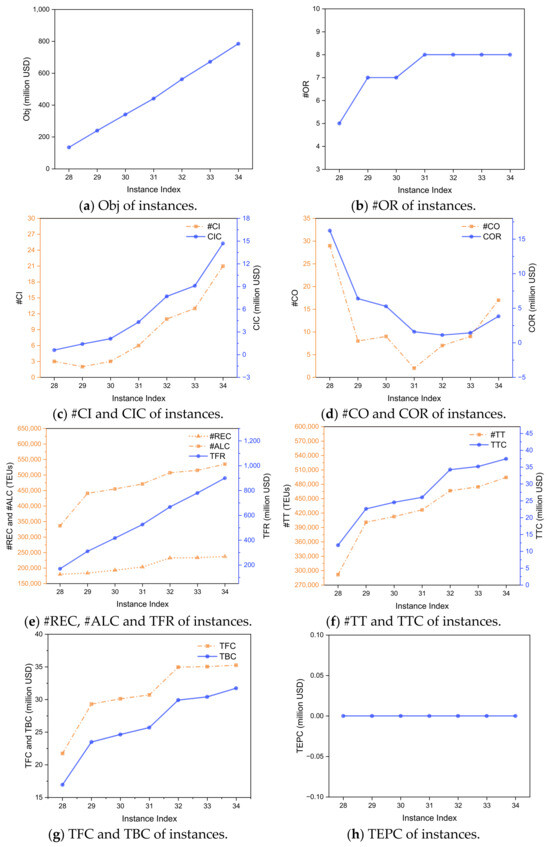
Figure 4.
Optimal results of the SRMIP model with different unit freight revenue percentages (Instance Index: 28–34).
As shown in Figure 4a, Obj increases almost linearly with the unit freight revenue percentage, which is consistent with our intuition, as higher per-container revenue directly translates to greater overall profitability. The increase in unit freight revenue percentage makes previously unprofitable routes profitable and incentivizes the model to operate more routes. As a result, #OR increases initially, as shown in Figure 4b. However, the #OR eventually reaches a plateau because further route expansion no longer effectively serves additional transport demand across more port pairs, or requires significantly higher unit freight revenue to make these new routes profitable.
The increase in the unit freight revenue percentage necessitates adjustments in fleet management. Initially, as #OR increases, more vessels are required to meet the fleet demand, resulting in an increase in #CI and a decrease in #CO, as shown in Figure 4c,d. When #OR stabilizes and the unit freight revenue percentage continues to rise, the model shifts to using vessels with larger transport capacity to carry more containers. This leads to an increase in both #CI and CIC, as the company leases in larger vessels, and a rise in #CO and COR as some smaller vessels are leased out.
The increase in #OR allows more routes to be interconnected through common ports, enabling more transport demand to be met. Additionally, as the unit freight revenue percentage increases, both the fleet size and the proportion of larger vessels in the fleet rise. Consequently, #REC, #ALC, TFR, #TT, TTC, TFC, and TBC all increase, as shown in Figure 4e–g.
Figure 4h shows that TEPC remains at 0 across all experiments in this group, which indicates that the model consistently identifies an optimal vessel assignment strategy, effectively avoiding the deployment of CN-constructed vessels on routes that would incur extra fees at US ports. It also highlights the relatively high extra fee, which drives the model to minimize avoidable penalty costs.
4.3.2. Sensitivity Analysis on the Unit Transit Cost Percentage
To investigate the impact of varying the transit cost on the model’s effectiveness, we design instances by altering the unit transit cost percentage from 0.4 to 1.6 while keeping the unit freight revenue percentage (), the unit fuel price (), and the unit extra fee () unchanged.
The optimal solutions from the MIP model are in Table 16, while those from the SRMIP model are in Table 17.
Table 16.
Optimal results of the MIP model with different unit transit cost percentages (Instance Index: 7–13).
Table 17.
Optimal results of the SRMIP model with different unit transit cost percentages (Instance Index: 35–41).
The MIP and SRMIP models yield identical optimized results, while the SRMIP model demonstrates faster computation. Figure 5 shows the optimal results of the SRMIP model in Group 5.
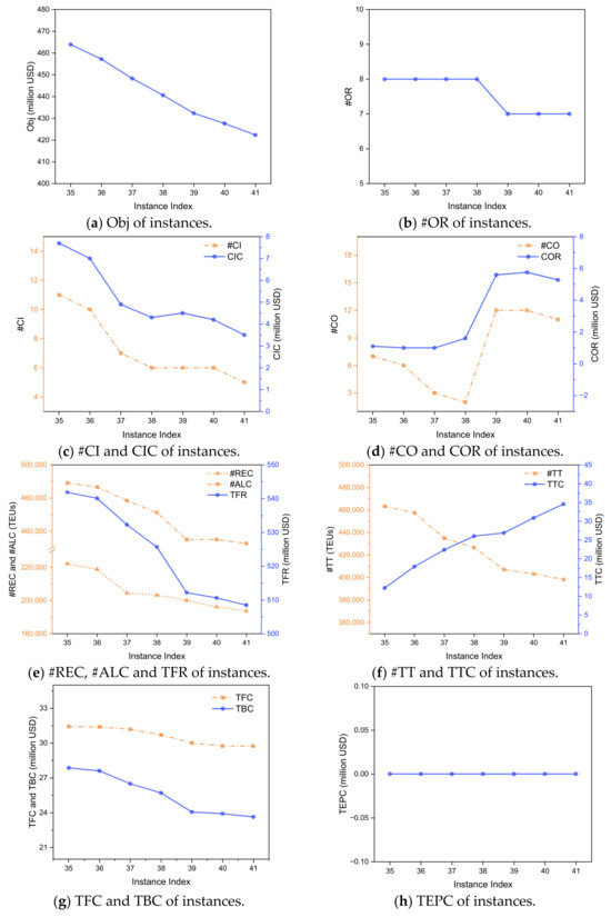
Figure 5.
Optimal results of the SRMIP model with different unit transit cost percentages (Instance Index: 35–41).
Figure 5a shows that as the unit transit cost percentage increases, Obj decreases steadily. This is expected, as the transit cost is a major cost component, and the increase in the unit transit cost percentage directly reduces the overall network profitability. As shown in Figure 5b, when the transit cost percentage becomes sufficiently high, #OR decreases. This indicates that, as the unit transit cost rises, certain routes which heavily rely on connecting transfer cargo become unprofitable.
As seen in Figure 5c–e, as the unit transit cost percentage increases, #CI and CIC show an overall downward trend, while #CO and COR generally increase. Similarly, #REC, #ALC, and TFR all decrease. This suggests that the model strategically reduces the acceptance of transport demand that relies on transshipment to cope with the rising costs. The decline in #TT with the increasing transit cost percentage, shown in Figure 5f, confirms this strategy. At the same time, TTC is observed to rise, which indicates that the increase in the unit transit cost outweighs the reduction in transshipped volume, resulting in a higher total transit cost. Especially, a significant change occurs at EID = 39, where #OR decreases from 8 to 7 (Figure 5b). Correspondingly, #CO increases sharply at EID = 39 (Figure 5d), while #ALC and TFR decrease significantly (Figure 5e). This indicates that the reduction in #OR reduces the required fleet size and leads to a substantial decrease in accepted transport demand.
Finally, Figure 5h shows that TEPC remains at 0 across all experiments in this group, which demonstrates that the model’s strategy to avoid the extra fees at US ports is consistently enforced, independent of transit cost fluctuations.
4.3.3. Sensitivity Analysis on the Unit Fuel Price
To investigate the impact of varying the unit fuel price on the model’s effectiveness, we design instances by altering the unit fuel price from 470 USD/ton to 650 USD/ton while keeping the unit freight revenue percentage (), the transit cost percentage (), and the unit extra fee () unchanged.
Table 18.
Optimal results of the MIP model with different unit fuel prices (Instance Index: 14–20).
Table 19.
Optimal results of the SRMIP model with different unit fuel prices (Instance Index: 42–48).
Table 18 and Table 19 display the numerical results for both the MIP and SRMIP models across different unit fuel prices, showing consistent trends in all indicators. The SRMIP model not only preserves the solution quality but also demonstrates a marked improvement in computational efficiency compared to the MIP model. Figure 6 illustrates the optimal results of the SRMIP model for Group 6.
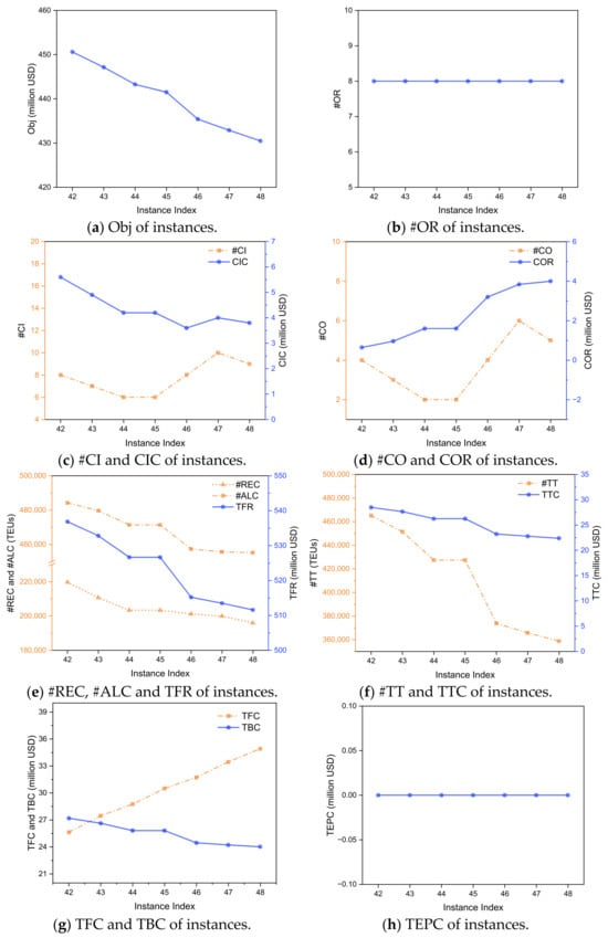
Figure 6.
Optimal results of the SRMIP model with different unit fuel prices (Instance Index: 42–48).
Figure 6a shows that as the unit fuel price increases, Obj decreases steadily, as fuel cost is a primary operational expense, and its increase directly reduces the overall network profitability. As shown in Figure 6b–d, #OR remains constant while #CI and #CO fluctuate as the unit fuel price increases. By referencing the data in Table 18 and Table 19, it is observed that the value of #CI minus #CO remains constant, which implies that the total number of vessels in the fleet is unchanged. This indicates that the model does not respond to rising fuel costs by changing the operation strategy. Instead, it adapts by optimizing fleet deployment.
Since smaller vessels consume less fuel, the model replaces some larger vessels in the fleet with smaller ones to reduce total fuel consumption. This change in fleet composition leads to a reduction in the network’s overall transport capacity, which in turn causes the observed decline in #REC, #ALC, and TFR, as shown in Figure 6e. The decrease in #ALC and #REC also leads to a reduction in the number of transshipments, which is confirmed by Figure 6f, showing that both #TT and TTC decline. Similarly, as the fleet composition shifts towards smaller vessels, the berthing costs decrease. However, the savings from reduced fuel consumption are not enough to offset the substantial rise in the unit fuel price. As a result, Figure 6g shows that TBC decreases slightly, while TFC increases significantly.
Finally, Figure 6h shows that TEPC remains at 0 across all experiments in this group, which consistently demonstrates the model’s robustness in finding an optimal vessel assignment that completely avoids the extra fees at US ports, even under the pressure of rising fuel costs.
4.3.4. Sensitivity Analysis on the Unit Extra Fee
To examine the effect of varying the extra fee on the model’s performance, we design test cases by adjusting the unit extra fee from 0 USD/TEU to 120 USD/TEU while keeping the unit freight revenue percentage (), the unit transit cost percentage (), and the unit fuel price () constant.
Table 20.
Optimal results of the MIP model with different unit extra fee (Instance Index: 21–27).
Table 21.
Optimal results of the SRMIP model with different unit extra fee (Instance Index: 49–55).
The results of varying the unit fuel price for both the MIP and SRMIP models are documented in Table 20 and Table 21, showing consistent trends across all indicators. Additionally, the SRMIP model achieves the same solution quality as the MIP model, while offering significantly higher computational efficiency. Figure 7 shows the optimal results of the SRMIP model in Group 7.
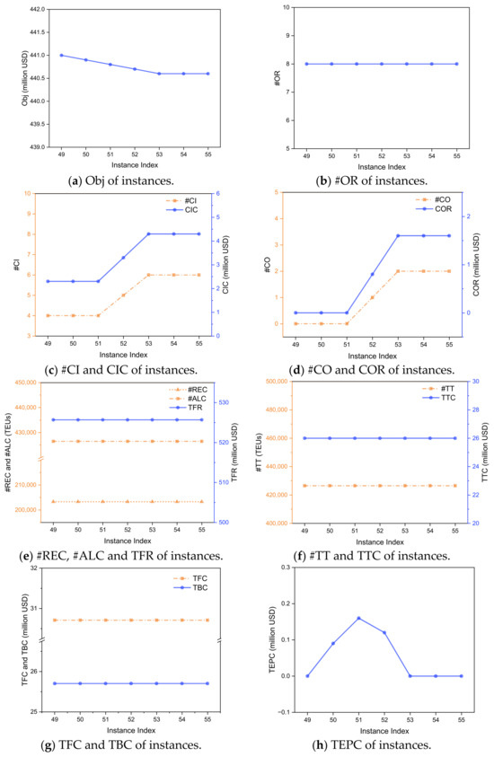
Figure 7.
Optimal results of the SRMIP model with different unit extra fee (Instance Index: 49–55).
Figure 7a shows that as the unit extra fee increases, Obj decreases. The most critical finding is in Figure 7h, which reveals the model’s adaptive strategy. When the unit extra fee is low, #CI and #CO remain constant (Figure 7c,d) while TEPC rises. This indicates that at low extra fee levels, it is more profitable to pay the penalty than to reconfigure the fleet by swapping CN-constructed vessels. However, as the unit extra fee continues to increase, TEPC reaches a peak and then begins to decline, which corresponds with a rise in #CI and #CO. This marks a critical tipping point where the economic trade-off shifts, and it becomes more advantageous to start swapping vessels to avoid the penalty cost. Once the unit extra fee is sufficiently high, TEPC drops to zero, and #CI and #CO stabilize at new, higher levels. At this stage, the model’s optimal strategy is to completely avoid the extra fees by ensuring non-CN-constructed vessels call at US ports.
Notably, this significant fleet reconfiguration has no discernible impact on the network’s operational performance. Figure 7b shows that #OR remains constant. Furthermore, key indicators including #REC, #ALC, TFR, #TT, TTC, TFC, and TBC all remain constant across all experiments in this group, as shown in Figure 7e–g. This demonstrates that the model executes an effective fleet swap, replacing the penalized vessels without altering the route operation strategy and transport volume.
4.3.5. Two-Factor Joint Sensitivity Analysis
Beyond the single-parameter sensitivity experiments, we further introduce a two-factor joint sensitivity analysis to better capture realistic market conditions where multiple parameters fluctuate simultaneously. This extension allows us to examine the combined effects of cost and revenue variations on network performance, providing a more comprehensive assessment of model robustness. In this analysis, we examine three types of joint perturbations, where the unit freight revenue percentage is considered together with the unit transit cost percentage, the unit fuel price, and the unit extra fee, respectively. For each of these experiments, two performance indicators are reported: Obj value and #ALC, which reflect the system’s profitability and service scale. The results of the three two-factor analyses are summarized in Figure 8, Figure 9 and Figure 10, where each figure displays the impacts of joint parameter variations on both Obj value and #ALC.
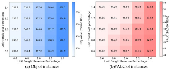
Figure 8.
Optimal results under joint sensitivity of freight revenue and transit cost.
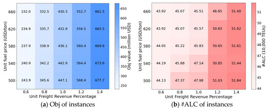
Figure 9.
Optimal results under joint sensitivity of freight revenue and fuel price.
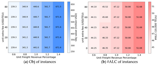
Figure 10.
Optimal results under joint sensitivity of freight revenue and extra fee.
Figure 8, Figure 9 and Figure 10 present the optimal results of the joint sensitivity analyses, where the unit freight revenue percentage is considered together with the unit transit cost percentage (Figure 8), the unit fuel price (Figure 9), and the unit extra fee (Figure 10). In all cases, Obj increases substantially with higher freight revenue, as transport operations that were previously unprofitable become profitable and both transport volume and unit revenue expand. By contrast, increases in transit costs and fuel prices reduce Obj when freight revenue is held constant, although their effects are moderate relative to the dominant role of freight revenue. The influence of extra fees on Obj is limited, as the model can offset most of these additional costs through leasing strategies that reduce or avoid penalty exposure for CN-constructed vessels.
The results for #ALC show consistent patterns. Higher freight revenue systematically increases #ALC, reflecting the system’s greater capacity to accommodate transport demand when unit revenues rise. At the same freight revenue level, transit costs exert a pronounced effect on #ALC: higher transit costs render some multi-transshipment flows unprofitable, leading the system to reject these demands and thereby reducing #ALC. Fuel prices also have a discernible impact, as higher fuel expenditures constrain the ability to accommodate marginal flows. Extra fees, in contrast, exert only a marginal effect on #ALC, since leasing adjustments enable the system to limit exposure to such penalties. Overall, freight revenue emerges as the primary driver of profitability and demand acceptance, while transit costs and fuel prices represent secondary but meaningful factors, and extra fees remain a marginal consideration within the tested ranges.
4.3.6. Summary and Managerial Insights
In conclusion, the numerical experiments, which explore variations in the unit freight revenue percentage, unit transit cost percentage, unit fuel price, and unit extra fee, clearly show that while both the MIP and SRMIP models produce identical optimal solutions, the SRMIP model achieves this with a remarkable increase in computational efficiency, effectively validating Theorem 1.
Through the experiments, we validate the effectiveness of the SRMIP model and derive several managerial insights that can help shipping companies make more effective tactical decisions in a dynamic market environment. We specifically found the following: (i) when market conditions are favorable with high freight revenues, companies should evaluate operating new routes as they may become profitable. Simultaneously, they should consider leasing in additional, and often larger, vessels to maximize the capture of profitable transport demand; (ii) when transshipment costs increase, companies should prioritize direct routing for cargo. This means the company should reduce the acceptance of transport demand requiring multiple transfers, as this cargo is the most sensitive to the transit cost increases and will be the first to become unprofitable. If a service route’s profitability is heavily dependent on connecting this transfer cargo, a significant rise in transshipment costs can make the entire service operate at a loss. In such cases, the company must consider discontinuing the route to avoid further financial losses. This strategic reduction is critical to avoid a potential cost trap: a sharp increase in unit transit costs can lead to higher total transshipment expenditures, even if the company is handling fewer transshipped containers overall; (iii) when fuel prices increase, companies should optimize fleet composition. Swapping vessels for more fuel-efficient ones on existing routes is an effective strategy to control total fuel expenditure, even if it may results in a slight reduction in overall transport capacity and accepted transport volume; (iv) when confronting policy-driven penalties, such as the extra fee for CN-constructed vessels above 4000 TEUs calling at US ports, a flexible leasing strategy is crucial. Companies must weigh the cost of paying the penalty against the cost of reconfiguring the fleet. As the extra fees become significant, leasing in compliant vessels while leasing out non-compliant ones is an effective way to eliminate the penalty, often without impacting network operations; (v) companies should prioritize freight revenue as the main driver of profitability, while controlling fuel, transshipment, and extra fees through fleet adjustments and flexible leasing.
This framework is particularly applicable to the determination of long-term stable liner networks, where carriers evaluate weekly net profit under relatively fixed service conditions. While demand fluctuations and speed adjustments do occur in practice, such short-term variations do not generally lead to structural changes in route configuration or fleet deployment. As a result, modeling demand and speed as fixed provides a valid representation of the stable decision horizon faced by carriers. If stochastic demand and vessel speed optimization are considered, additional managerial insights can be obtained. When demand is uncertain, companies should use flexible leasing contracts and keep some spare capacity to handle fluctuations without taking on too much risk. If vessel speed is treated as a decision variable, managers must weigh cost efficiency against schedule reliability, since changes in speed directly affect fuel use and the number of vessels needed to maintain weekly services. These considerations further emphasize the importance of adaptive strategies in dynamic markets.
5. Conclusions
Liner shipping companies operate in a highly competitive and complex global market. They face the constant challenge of designing profitable service networks by making a series of critical, interdependent tactical decisions. These include deploying a heterogeneous fleet, managing vessel leasing and transshipment activities, accepting or rejecting transport demand, and effectively repositioning empty containers to balance profitability with equipment availability. The complexity is further compounded by volatile operational costs and the increasing influence of trade-related policies that can impose significant financial penalties. In this context, using data-driven methods for shipping network decision-making is crucial, as it enables companies to navigate the complexities of their operations and make more informed, efficient decisions. By leveraging real-time data and advanced analytics, companies can better optimize their fleet deployment, manage costs, and respond to market fluctuations effectively.
Building on the above facts, we develop a MIP model for the LSND–CFM problem. The model simultaneously optimizes route selection, vessel assignment, laden container acceptance and empty container repositioning considering transshipment, and fleet leasing decisions. Furthermore, we establish a theorem to prove that the original MIP model can be transformed into a SRMIP model by relaxing the integer variables for vessel leasing. This theoretical contribution demonstrates how exploiting the TU property of constraint structures allows partial relaxation of integer variables without compromising solution integrality. Beyond our specific case, this insight provides a methodological reference for other large-scale transportation and logistics optimization problems, such as airline fleet assignment, railway scheduling, and intermodal transport planning, where subsets of decision variables may exhibit TU characteristics. By identifying and leveraging such properties, researchers and practitioners can design semi-relaxed formulations that achieve substantial computational savings while preserving exactness.
In the numerical experiments, a real-world case study is employed to validate the model’s effectiveness. The basic results demonstrate the model’s capability to generate a highly profitable operational plan that effectively mitigates policy-driven penalty costs. The sensitivity analyses further reveal valuable insights into the model’s strategic responses to market dynamics. The results show that the optimal strategy involves expanding the service network by operating more routes in markets with high freight revenue, adjusting the service network by discontinuing routes that rely heavily on transshipment when the transit cost increases, adjusting fleet composition to manage fuel price volatility, and leveraging leasing to navigate trade-related financial penalties.
Although the proposed optimization framework shows significant promise in supporting tactical decision-making, it has some limitations. Future research could focus on the following areas for further improvement.
- Idealized assumptions and real-world applicability: The current framework relies on several idealized assumptions, including deterministic transport demand, fixed vessel speeds, and a static regulatory and cost environment (e.g., carbon emission taxes). While these simplifications facilitate model tractability and highlight core contributions, they inevitably overlook the inherent real-world volatility of market fluctuations, the operational flexibility in vessel speed, and the dynamic nature of environmental regulations and associated costs. Future research will focus on the following: developing stochastic programming or robust optimization models to incorporate demand uncertainty [53,54]; integrating vessel speed as a decision variable to analyze trade-offs between fuel consumption, transit time, and fleet size [55,56]; and extending the model to include flexible regulatory policies and additional charges [57,58]. This will significantly enhance the framework’s adaptability to dynamic market environments and evolving maritime regulations.
- Addressing scalability challenges for large-scale systems: Our current methodology, while effective for the scenarios studied, faces inherent computational challenges when applied to increasingly larger or more complex real-world maritime transportation networks. Expanding its applicability requires a strong focus on improving scalability. For instance, future work can delve into advanced decomposition techniques, metaheuristic approaches, or parallel computing paradigms to efficiently solve the large-scale optimization problems inherent in global shipping networks. This would relax the implicit assumption of manageable problem size and broaden the method’s practical utility [59,60].
- Incorporating adaptive and learning-based mechanisms: The sensitivity of optimization methods to initial conditions and parameter tuning is a critical practical concern. Future work could significantly strengthen the approach by incorporating adaptive or learning-based mechanisms. This involves developing frameworks that can dynamically adjust model parameters or even adapt solution strategies based on real-time operational data or observed system performance. Machine learning techniques, particularly reinforcement learning or adaptive control, offer promising avenues for achieving greater robustness and responsiveness in complex, uncertain maritime environments [61,62].
Author Contributions
Conceptualization, S.W.; methodology, Y.T., Y.Y. and S.W.; software, Y.T.; validation, Y.T.; formal analysis, Y.T.; investigation, Y.T., Y.Y. and S.W.; resources, S.W.; data curation, Y.T. and Y.Y.; writing—original draft preparation, Y.T., Y.Y. and S.W.; writing—review and editing, Y.T., Y.Y. and S.W.; visualization, Y.T.; supervision, S.W.; project administration, S.W.; funding acquisition, S.W. All authors have read and agreed to the published version of the manuscript.
Funding
This research received no external funding.
Data Availability Statement
The raw data supporting the conclusions of this article will be made available by the authors on request.
Conflicts of Interest
The authors declare no conflicts of interest.
References
- Zhao, Y.; Chen, Z.; Lim, A.; Zhang, Z. Vessel deployment with limited information: Distributionally robust chance constrained models. Transp. Res. Part B 2022, 161, 197–217. [Google Scholar] [CrossRef]
- Karsten, C.V.; Pisinger, D.; Ropke, S.; Brouer, B.D. The time constrained multi-commodity network flow problem and its application to liner shipping network design. Transp. Res. Part E 2015, 76, 122–138. [Google Scholar] [CrossRef]
- Revised US Port Fee Plan Leaves Important Questions Unanswered, Lawyers Argue. Available online: https://www.lloydslist.com/LL1153244/Revised-US-port-fee-plan-leaves-important-questions-unanswered-lawyers-argue (accessed on 9 June 2025).
- The U.S. Shipbuilding Industry vs. China and the Issue of Port Tariffs. Available online: https://www.thesignalgroup.com/newsroom/the-u-s-shipbuilding-industry-vs-china-and-the-issue-of-port-tariffs (accessed on 9 June 2025).
- US Revises Port Fees for Chinese-Constructed Ships Amid Industry Concerns. Available online: https://www.ship-technology.com/news/us-rport-fees-for-china-ships/ (accessed on 9 June 2025).
- Nadarajan, D.; Ahmed, S.A.M.; Noor, N.F.M. Seaport network efficiency measurement using triangular and trapezoidal fuzzy data envelopment analyses with liner shipping connectivity index output. Mathematics 2023, 11, 1454. [Google Scholar] [CrossRef]
- Wang, S.; Meng, Q. Liner ship fleet deployment with container transshipment operations. Transp. Res. Part E 2012, 48, 470–484. [Google Scholar] [CrossRef]
- Notteboom, T.; Haralambides, H.; Cullinane, K. The Red Sea Crisis: Ramifications for vessel operations, shipping networks, and maritime supply chains. Marit. Econ. Logist. 2024, 26, 1–20. [Google Scholar] [CrossRef]
- Baird, A.J. Optimising the container transhipment hub location in northern Europe. J. Transp. Geogr. 2006, 14, 195–214. [Google Scholar] [CrossRef]
- Song, D.P.; Carter, J. Empty container repositioning in liner shipping. Marit. Policy Manag. 2009, 36, 291–307. [Google Scholar] [CrossRef]
- Chen, K.; Lu, Q.; Xin, X.; Yang, Z.; Zhu, L.; Xu, Q. Optimization of empty container allocation for inland freight stations considering stochastic demand. Ocean Coast. Manag. 2022, 230, 106366. [Google Scholar] [CrossRef]
- Abdelshafie, A.; Salah, M.; Kramberger, T.; Dragan, D. Repositioning and optimal re-allocation of empty containers: A review of methods, models, and applications. Sustainability 2022, 14, 6655. [Google Scholar] [CrossRef]
- Wang, W.; Yang, Z.; Diao, C.; Jin, Z. Collaborative optimization of container liner slot allocation and empty container repositioning based on online booking platform. Appl. Sci. 2024, 14, 11092. [Google Scholar] [CrossRef]
- Tao, Y.; Yang, Y.; Wang, S. Managing surcharge risk in strategic fleet deployment: A partial relaxed MIP model framework with a case study on China-built ships. Appl. Sci. 2025, 15, 8582. [Google Scholar] [CrossRef]
- Brouer, B.D.; Alvarez, J.F.; Plum, C.E.; Pisinger, D.; Sigurd, M.M. A base integer programming model and benchmark suite for liner-shipping network design. Transp. Sci. 2014, 48, 281–312. [Google Scholar] [CrossRef]
- Branchini, R.M.; Armentano, V.A.; Morabito, R. Routing and fleet deployment in liner shipping with spot voyages. Transp. Res. Part C 2015, 57, 188–205. [Google Scholar] [CrossRef]
- Gelareh, S.; Meng, Q. A novel modeling approach for the fleet deployment problem within a short-term planning horizon. Transp. Res. Part E 2010, 46, 76–89. [Google Scholar] [CrossRef]
- Notteboom, T.E. The time factor in liner shipping services. Marit. Econ. Logist. 2006, 8, 19–39. [Google Scholar] [CrossRef]
- Tran, N.K.; Haasis, H.D. An empirical study of fleet expansion and growth of ship size in container liner shipping. Int. J. Prod. Econ. 2015, 159, 241–253. [Google Scholar] [CrossRef]
- Wetzel, D.; Tierney, K. Integrating fleet deployment into liner shipping vessel repositioning. Transp. Res. Part E 2020, 143, 102101. [Google Scholar] [CrossRef]
- Hong, Q.; Tian, X.; Li, H.; Liu, Z.; Wang, S. Sample distribution approximation for the ship fleet deployment problem under random demand. Mathematics 2025, 13, 1610. [Google Scholar] [CrossRef]
- Elmi, Z.; Singh, P.; Meriga, V.K.; Goniewicz, K.; Borowska-Stefańska, M.; Wiśniewski, S.; Dulebenets, M.A. Uncertainties in liner shipping and ship schedule recovery: A state-of-the-art review. J. Mar. Sci. Eng. 2022, 10, 563. [Google Scholar] [CrossRef]
- Qu, H.; Wang, X.; Meng, L.; Han, C. Liner schedule design under port congestion: A container handling efficiency selection mechanism. J. Mar. Sci. Eng. 2024, 12, 951. [Google Scholar] [CrossRef]
- Koza, D.F.; Desaulniers, G.; Ropke, S. Integrated liner shipping network design and scheduling. Transp. Sci. 2020, 54, 512–533. [Google Scholar] [CrossRef]
- Psaraftis, H.N.; Kontovas, C.A. Speed models for energy-efficient maritime transportation: A taxonomy and survey. Transp. Res. Part C 2013, 26, 331–351. [Google Scholar] [CrossRef]
- Kuzmicz, K.A.; Pesch, E. Approaches to empty container repositioning problems in the context of Eurasian intermodal transportation. Omega 2019, 85, 194–213. [Google Scholar] [CrossRef]
- Ross, A.D.; Jayaraman, V.; Rodrigues, A.; Mollenkopf, D.A. Repositioning of reusable containers in a sustainable global supply chain environment. Int. J. Math. Oper. Res. 2010, 2, 178–204. [Google Scholar] [CrossRef]
- Shintani, K.; Imai, A.; Nishimura, E.; Papadimitriou, S. The container shipping network design problem with empty container repositioning. Transp. Res. Part E 2007, 43, 39–59. [Google Scholar] [CrossRef]
- Montes-Franco, A.M.; Martinez-Franco, J.C.; Tabares, A.; Álvarez-Martínez, D. A hybrid approach for the container loading problem for enhancing the dynamic stability representation. Mathematics 2025, 13, 869. [Google Scholar] [CrossRef]
- Meng, Q.; Wang, S.; Andersson, H.; Thun, K. Containership routing and scheduling in liner shipping: Overview and future research directions. Transp. Sci. 2014, 48, 265–280. [Google Scholar] [CrossRef]
- Christiansen, M.; Hellsten, E.; Pisinger, D.; Sacramento, D.; Vilhelmsen, C. Liner shipping network design. Eur. J. Oper. Res. 2020, 286, 1–20. [Google Scholar] [CrossRef]
- Huang, X.; Chen, H.; Zhang, J.; Wang, D.; Chen, J.; Luo, J.X. Robust optimization model of container liner routes in feeder line network. Transport 2024, 39, 13–24. [Google Scholar] [CrossRef]
- Abioye, O.F.; Dulebenets, M.A.; Pasha, J.; Kavoosi, M. A vessel schedule recovery problem at the liner shipping route with emission control areas. Energies 2019, 12, 2380. [Google Scholar] [CrossRef]
- Hoffman, A.J.; Kruskal, J.B. Integral boundary points of convex polyhedra. In 50 Years of Integer Programming 1958–2008: From the Early Years to the State-of-the-Art; Springer: Berlin/Heidelberg, Germany, 2010; pp. 49–76. [Google Scholar] [CrossRef]
- Ocean Alliance 2025 Service Network. Available online: https://container-news.com/ocean-alliance-rolls-out-new-service-network-2/ (accessed on 9 June 2025).
- Ocean Carrier Alliances 2025. Available online: https://www.shipit.com/post/ocean-carrier-alliances-2025-a-complete-guide-to-the-new-shipping-networks (accessed on 9 June 2025).
- Sea-Intelligence, Asia-NAM and Asia-Europe Networks Impact 2025. Available online: https://sea-intelligence.com/press-room/286-asia-nam-and-asia-europe-networks-impact-2025 (accessed on 9 June 2025).
- Clarksons Charter Market Reports. Available online: https://www.clarksons.net/ (accessed on 9 June 2025).
- World Shipping Council, Top 50 World Container Ports. Available online: https://www.worldshipping.org/top-50-container-ports (accessed on 9 June 2025).
- Maersk East-West Network. Available online: https://www.maersk.com/east-west-network (accessed on 9 June 2025).
- Record Wave of New Containerships in 2024. Available online: https://gcaptain.com/record-wave-of-new-containerships-in-2024/ (accessed on 9 June 2025).
- Perspectives on Reefer Containers. Available online: https://www.sciencedirect.com/science/article/abs/pii/S0924224423002625 (accessed on 9 June 2025).
- Container Shipping Statistics. Available online: https://www.statista.com/statistics/1103135/container-shipping-market-size-worldwide/ (accessed on 9 June 2025).
- COSCO Container’s Number of Ships. Available online: https://www.statista.com/statistics/199369/number-of-ships-of-cosco-container-l-in-december-2011/ (accessed on 9 June 2025).
- COSCO Shipping Holdings Announced 2024 Annual Results. Available online: http://en.hold.coscoshipping.com/col/col25402/art/2025/art_62bab154a21547b0a5d2ee0ce9bdfd97.html (accessed on 9 June 2025).
- Big Variances to Chinese-Constructed Boxship Exposure for US Service Providers. Available online: https://www.lloydslist.com/LL1152761/Big-variances-to-Chinese-constructed-boxship-exposure-for-US-service-providers (accessed on 9 June 2025).
- Freightos Baltic Index Global Container Pricing. Available online: https://terminal.freightos.com/freightos-baltic-index-global-container-pricing-index/ (accessed on 9 June 2025).
- Xeneta Shipping Index Container Freight Market. Available online: https://xsi.xeneta.com (accessed on 9 June 2025).
- Drewry World Container Index. Available online: https://www.drewry.co.uk/supply-chain-advisors/supply-chain-expertise/world-container-index-assessed-by-drewry (accessed on 9 June 2025).
- Wang, S.; Meng, Q. Sailing speed optimization for container ships in a liner shipping network. Transp. Res. Part E 2012, 48, 701–714. [Google Scholar] [CrossRef]
- Global 20 Ports Average Bunker Prices. Available online: https://shipandbunker.com/prices/av/global/av-g20-global-20-ports-average (accessed on 10 June 2025).
- LLC Schedule of Rates No. 1. 2022. Available online: https://www.portofvirginia.com/wp-content/uploads/2023/09/SOR-Original-10.01.22v4-1.pdf (accessed on 9 June 2025).
- Liu, B.; Li, Z.C.; Wang, Y. A two-stage stochastic programming model for seaport berth and channel planning with uncertainties in ship arrival and handling times. Transp. Res. Part E 2022, 167, 102919. [Google Scholar] [CrossRef]
- Santos, A.M.P.; Fagerholt, K.; Laporte, G.; Soares, C.G. A stochastic optimization approach for the supply vessel planning problem under uncertain demand. Transp. Res. Part B 2022, 162, 209–228. [Google Scholar] [CrossRef]
- Li, X.; Sun, B.; Jin, J.; Ding, J. Speed optimization of container ship considering route segmentation and weather data loading: Turning point-time segmentation method. J. Mar. Sci. Eng. 2022, 10, 1835. [Google Scholar] [CrossRef]
- Li, X.; Gu, Y.; Fan, X.; Zou, K.; Hou, X. An optimization model for ship speed based on maneuvering control. J. Mar. Sci. Eng. 2022, 11, 49. [Google Scholar] [CrossRef]
- Deng, S.; Mi, Z. A review on carbon emissions of global shipping. Mar. Dev. 2023, 1, 4. [Google Scholar] [CrossRef]
- Cariou, P.; Halim, R.A.; Rickard, B.J. Ship-owner response to carbon taxes: Industry and environmental implications. Ecol. Econ. 2023, 212, 107917. [Google Scholar] [CrossRef]
- Chen, W.; Men, Y.; Fuster, N.; Osorio, C.; Juan, A.A. Artificial intelligence in logistics optimization with sustainable criteria: A review. Sustainability 2024, 16, 9145. [Google Scholar] [CrossRef]
- Abdalsalam, M.; Szłapczyńska, J. Towards improved ship weather routing through multi-objective optimization with high performance computing support. TransNav-Int. J. Mar. Navig. Saf. Sea Transp. 2025, 19, 93–103. [Google Scholar] [CrossRef]
- Lu, Y. A multimodal deep reinforcement learning approach for IoT-driven adaptive scheduling and robustness optimization in global logistics networks. Sci. Rep. 2025, 15, 25195. [Google Scholar] [CrossRef]
- Lv, Y.; Gao, Y.; Liu, J. Dual strategies-based resilience enhancement in a bulk cargo port under dynamic machinery failure scenarios with reinforcement learning. Ocean Coast. Manag. 2025, 260, 107484. [Google Scholar] [CrossRef]
Disclaimer/Publisher’s Note: The statements, opinions and data contained in all publications are solely those of the individual author(s) and contributor(s) and not of MDPI and/or the editor(s). MDPI and/or the editor(s) disclaim responsibility for any injury to people or property resulting from any ideas, methods, instructions or products referred to in the content. |
© 2025 by the authors. Licensee MDPI, Basel, Switzerland. This article is an open access article distributed under the terms and conditions of the Creative Commons Attribution (CC BY) license (https://creativecommons.org/licenses/by/4.0/).