Abstract
To address the impact of the dynamic evolution of flood disaster chains and decision-makers’ (DMs’) risk preference heterogeneity on group decision-making, this study proposes a social network group decision-making method that integrates the evolutionary trend of the flood disaster chain with DMs’ risk preferences. First, a Bayesian network is constructed to quantify the disaster chain’s evolution, dynamically adjusting DMs’ evaluation values. Second, DMs’ risk preference types are identified based on the evaluation values, and a bounded confidence (BC) model, incorporating risk preferences, self-confidence and trust networks, is developed to promote consensus formation. Then, the optimal alternative is selected through weighted aggregation and used to update the Bayesian network dynamically during implementation. Finally, the effectiveness and superiority of the proposed method are verified using the flood disaster chain from the “7∙20” extreme rainfall disaster in Zhengzhou, Henan Province, China. The results show that risk-seeking DMs reduce BC values and resist consensus, whereas risk-averse DMs enlarge BC values and accelerate convergence. Moreover, worsening flood disaster chain trends drive DMs to update the optimal alternative. These findings show that the method captures both dynamic disaster evolution and behavioral heterogeneity, providing realistic and adaptive decision support in flood emergency scenarios.
Keywords:
flood disaster chain; Bayesian network; triangular intuitionistic fuzzy numbers; social network group decision making; bounded confidence model MSC:
91B06
1. Introduction
In recent years, influenced by global climate change and accelerated urbanization, the frequency and intensity of flood disasters have increased significantly. These events often trigger a series of secondary disasters, forming complex flood disaster chains characterized by cascading, compounding, and amplifying effects. Such chains pose severe threats to urban infrastructure, public safety, and the stability of socio-economic systems [1,2,3]. For example, from 11 to 12 April 2024, Afghanistan and Pakistan were hit by heavy rainfall, causing widespread flooding that inundated rivers, submerged farmland, destroyed homes, and disrupted transportation, affecting over 830,000 people and resulting in the death of approximately 178,000 livestock. From 28 to 30 October 2024, torrential rains and hailstorms struck eastern and southern Spain, leading to severe floods that caused at least 226 fatalities. In the Valencia region, extensive disruptions in telecommunications and internet services occurred, 150 roads were paralyzed, critical infrastructure was heavily damaged, over 150,000 households lost power, and direct economic losses exceeded €3.5 billion [4].
A flood disaster chain typically comprises multiple causally linked hazard events and exhibits a domino-like effect. It is commonly triggered by a primary flood event and subsequently leads to urban waterlogging, traffic paralysis, communication breakdowns, landslides, and other secondary disasters. These chains are cumulative, highly uncertain, and challenging to predict and control, with destructive potential far exceeding that of isolated hazards [5,6,7]. Moreover, traditional group decision-making (GDM) methods often overlook the heterogeneity of decision-makers’ (DMs’) risk preferences, disregarding their differentiated perceptions and value-adjustment behaviors during the decision process. Therefore, there is a pressing need for a GDM framework that integrates the evolutionary trend of flood disaster chains with DMs’ risk preferences, in order to enhance the scientific rigor and timeliness of emergency response under complex disaster scenarios.
To address these problems, this study proposes a social network group decision-making (SNGDM) method that integrates the evolutionary trends of flood disaster chains with the regulation of DMs’ risk preferences.
The remainder of this paper is organized as follows: Section 2 reviews related research. Section 3 introduces the theoretical foundations of Triangular Intuitionistic Fuzzy Numbers (TIFNs), Bayesian networks (BNs), and Trust Networks. Section 4 proposes a new SNGDM method that integrates the evolutionary trend of flood disaster chains with risk preferences, detailing the design and implementation of its key components. Section 5 illustrates a case study to demonstrate the effectiveness and feasibility of the proposed method in practical scenarios. Section 6 presents the sensitivity and comparative analyses. Finally, Section 7 concludes the study and outlines directions for future research.
2. Literature Review
2.1. Disaster Chain Modeling
To address the cascading evolution of flood disaster chains, BNs have been widely employed to model causal relationships among disaster events and estimate the occurrence probabilities of secondary disasters [5,8,9]. For example, Guo et al. [10] developed a BN model for storm surge disaster chains to predict the evolution of complex disaster networks and estimate the occurrence probabilities of events and associated loss scenarios. Zhang et al. [11] employed BNs to characterize the intricate processes and probabilistic features of urban flooding, thereby assessing flood risks in urban settings. Mohammadi et al. [12] integrated multi-source data to construct a joint probability distribution of flood-driving mechanisms using a BN model. However, these studies mainly emphasize structural modeling and probabilistic inference, without quantitatively characterizing the evolutionary trends of the disaster chain.
In contrast, studies in other disaster prediction fields have applied diverse methods to quantify dynamic hazard impacts. In communication networks, Zhang et al. [13] proposed an interference optimization algorithm for the Multi-layer Model of Network Dissemination to determine optimal network parameters, enabling rapid disaster information dissemination. In public health, Lan et al. [14] employed distributed lag models to quantify flood effects on diarrheal morbidity. In geotechnical and hydraulic engineering, Zheng et al. [15] used the Material Point Method to simulate levee failure under combined heavy rainfall and high river levels, providing a quantitative stability assessment, while Huang et al. [16] developed a method to estimate dam-break flood pressures under high Froude number conditions. In earthquake and geological hazard studies, Xu et al. [17] proposed a spatiotemporal casualty assessment method that incorporates human emergency behavior to predict community-scale casualties, and Liu et al. [18] employed three-dimensional discontinuous deformation analysis to simulate rockfall dynamics, including block movement, kinetic energy, and impact interactions. These examples demonstrate the value of integrating dynamic quantification into disaster chain modeling.
2.2. Group Decision-Making Under Uncertainty
Accurately representing DMs’ evaluation values is critical for addressing the uncertainty in flood disaster chain decision-making. To capture subjective judgments and hesitation, TIFNs have been widely adopted as an effective tool for representing imprecise information in GDM scenarios [19,20,21]. For example, Lu et al. [22] integrated TIFNs, fuzzy measures, and the Choquet integral to rank alternatives. Huang et al. [23] proposed an intuitionistic fuzzy approach based on TIFNs and consensus measures to determine the weights of criteria, thereby reflecting their relative importance in GDM. However, most existing studies focus on the static representation of evaluation values and overlook the potential impact of disaster chain evolution on DMs’ evaluation values.
2.3. Social Network Group Decision Making
DMs form social networks based on trust relationships, facilitating the exchange of evaluation opinions and consensus coordination, thereby forming an SNGDM framework [24]. The consensus-reaching process, as a core component of SNGDM, typically employs dynamic iterative mechanisms to coordinate group evaluation opinions and enhance decision consistency [25]. With the increasing adoption of dynamic opinions, when the group consensus level fails to reach a predefined threshold, the bounded confidence (BC) model is often utilized to establish feedback mechanisms that promote the adjustment of evaluation values until the desired consensus is attained [26,27,28,29,30]. For instance, Zhou et al. [31] proposed a three-level consensus identification rule considering self-confidence, along with adjustment rules incorporating trust relationships, consensus degree, and reliability. However, their approach treats the BC value as a fixed parameter, neglecting the dynamic variations of DMs’ psychological acceptance during the consensus formation process. To address this limitation, Liu et al. [32] introduced an adaptive BC model that dynamically adjusts the BC value in response to changes in DMs’ willingness, thereby enhancing the model’s adaptability to evolving preferences. Nevertheless, existing studies have insufficiently accounted for the moderating effect of DMs’ risk preferences within the BC model. In practical SNGDM, outcomes are inevitably influenced by DMs’ risk attitudes [33,34]. Variations in risk perception toward the same alternative—characterized as risk-averse, risk-neutral, or risk-seeking behaviors—and differences in stress tolerance and self-confidence directly influence the adjustment of evaluation values and the willingness to accept external feedback [35]. Prior research on risk preferences has predominantly focused on identifying herd behavior among DMs [35], characterizing risk-taking capabilities [36], and developing multi-objective portfolio selection models [37], but has yet to integrate these factors into the BC framework. This gap impedes the construction of consensus mechanisms that better align with actual behavioral patterns within groups.
2.4. Research Gaps and Novelty
Based on the above analysis, the main research gaps are as follows:
- (1)
- BN-based models of flood disaster chains focus on structural inference but lack a dynamic and quantitative assessment of evolutionary trends.
- (2)
- Existing GDM models rely on static evaluation values and fail to integrate disaster chain evolution, overlooking the necessity of dynamic adjustment in emergency contexts.
- (3)
- The BC model is a cornerstone of the consensus-reaching process. However, most implementations assume a homogeneous, risk-neutral attitude among DMs. In reality, DMs hold heterogeneous risk preferences that strongly influence their willingness to adjust opinions during the consensus-reaching process. Ignoring this factor diminishes the psychological realism and practical applicability of existing BC-based frameworks in complex, risk-driven scenarios like emergency management.
To address these gaps, this study proposes a new SNGDM method. The primary contributions of this study include the following:
- (1)
- Based on the inference results of the BNs, an evolutionary trend index of the flood disaster chain is constructed to enable a quantitative analysis of its evolution. This index is used both to adjust DMs’ evaluation values and to determine whether alternative adjustments are required.
- (2)
- A new BC model is proposed, which integrates DMs’ risk preferences, self-confidence, and trust networks. The BC model, where DMs adjust their opinions within a specified confidence threshold, forms the foundation of the consensus-reaching process in SNGDM. By incorporating DMs’ risk preferences, this BC model enhances the sensitivity and realism of consensus formation and provides a more robust approach to decision-making in flood disaster chain scenarios.
- (3)
- An intelligent closed-loop decision-making framework is constructed, incorporating scenario forecasting, alternative selection, and feedback-informed disaster evolution tracking.
These innovations enable the proposed SNGDM framework to outperform static or risk-neutral models by dynamically integrating disaster chain evolution with the heterogeneous risk preferences of DMs, thereby allowing for the dynamic adjustment of evaluation values and improving decision quality under diverse behavioral tendencies.
3. Methodology
This study proposes an SNGDM method integrating three components: TIFNs to represent DMs’ preferences and hesitation, BNs to model the probabilistic evolution of the flood disaster chain, and trust networks to capture interactions among DMs. First, a BN is constructed to quantify the evolution of the disaster chain and dynamically adjust DMs’ evaluation values, represented by TIFNs. Second, DMs’ risk preference types are identified from these evaluation values, and a BC model—incorporating risk preference, self-confidence and a trust network—is applied to promote consensus formation. The optimal alternative is then selected through weighted aggregation and used to update the BN during the implementation phase. The following subsections describe these components in detail and their integration within the overall framework. A summary of all abbreviations and symbols used in this paper is provided in Appendix A Table A1.
3.1. Triangular Intuitionistic Fuzzy Number
Definition 1
[38]. Let be a triangular intuitionistic fuzzy number (TIFN) defined on a real number set R, whose membership function and non-membership function are denoted as follows:
and
where and represent the maximum membership degree and the minimum non-membership degree of , respectively, such that they satisfy the conditions , and . Let represent the hesitation degree of the TIFN, where a smaller value indicates a higher level of certainty in the fuzzy number.
Definition 2
[38,39]. Let and be two TIFNs and be a real number. The arithmetical operations are stipulated as follows:
Definition 3
[40]. Let represent a TIFN, whose score function is defined as follows:
Its accuracy function is as follows:
Definition 4
[40]. Let and be two TIFNs, if , then . If , (1) when , then ; (2) when , then .
Definition 5
[19]. Let and be two TIFNs, then the Hamming distance between and can be defined as follows:
when , , and the TIFNs and
degraded into triangular fuzzy numbers (TFNs), the distance between them is simplified as follows:
Definition 6
[41]. Let be a collection of TIFNs, is the set of all TIFNs, and
is the weight of
satisfying that
and
. Then the TIF-WA operator is defined as follows:
3.2. Bayesian Network
BNs consist of nodes and directed edges, where each node represents a random variable, and the directed edges (from parent to child nodes) denote conditional dependencies. The strength of these dependencies is quantified using conditional probabilities.
Definition 7
[42,43]. The Let be a directed acyclic graph (DAG), where and denote the sets of nodes and directed edges, respectively. Let , represent the random variable associated with node in the DAG. The joint probability of node is given by the following:
where denotes the parent nodes of node .
3.3. Trust Network
Definition 8
[44]. In the decision-making process, a trust network is defined as a directed graph , where denotes the set of decision-makers, and is a mapping from . For any two decision-makers and in D, the trust degree of toward is represented by a trust probability . Accordingly, the trust relationships among all decision-makers can be represented in the form of a trust matrix , . A higher value of indicates that DM has greater trust in . It is assumed that each DM fully trusts themselves, .
4. Problem Description and Proposed Method
The integration of a BN and SNGDM represents a process that bridges disaster prediction with decision optimization. A BN is used to quantify the occurrence probabilities of disaster events, offering conditional probabilities and causal pathways within the disaster chain, thereby providing reliable predictive insights. SNGDM leverages this information to support decision-makers in comprehensively evaluating the advantages and disadvantages of multiple alternatives, while incorporating trust relationships to facilitate the selection of the optimal alternative.
The proposed framework proceeds as follows: First, at the early stage of a flood disaster, a BN model of the flood disaster chain is established to estimate the occurrence probabilities of each disaster event. This enables the quantitative assessment of the disaster chain’s evolutionary trend, leading to the derivation of a flood disaster chain evolutionary trend index. Second, this index is used to dynamically adjust the initial evaluation values. Based on the adjusted values, DMs’ risk preference types are identified, and their corresponding BC values are calculated to support the consensus-reaching process and determine the optimal alternative. Finally, as the disaster scenario evolves, real-time observational data are employed to update the BN structure and node states. The implementation outcomes of the selected response alternative are then fed back into the BN, allowing for updated occurrence probabilities of both primary and secondary disasters. This facilitates a reassessment of the current alternative and determines whether dynamic adjustments are necessary.
4.1. Problem Description
The flood disaster chain is a complex system composed of a series of secondary and derivative disasters triggered by a primary flood event. It is characterized by high dynamism and uncertainty. Compared with traditional single-disaster scenarios, SNGDM for flood disaster chains faces greater uncertainty and must also account for the interdependencies among various nodes within the chain. This results in a multi-stage evolutionary process with diverse impact pathways.
Specifically, flood disaster chains exhibit three prominent features:
- (1)
- Cascading propagation: A primary flood event can trigger multiple levels of secondary disasters, forming a typical cascade evolution structure;
- (2)
- Time-varying uncertainty: The conditional probability parameters governing disaster propagation are influenced by real-time environmental factors such as meteorological and hydrological conditions, leading to highly dynamic behavior;
- (3)
- Intervention feedback: alternatives not only affect the current disaster mitigation outcomes but may also feed back into the disaster chain, altering its subsequent evolutionary trajectory.
Based on the above characteristics, SNGDM models should shift from the traditional “passive response” approach to a more proactive “prevention and control” strategy. Priority should be given to rapid response in the early stages of flood disasters to contain the event at its source, thereby preventing its escalation and interrupting the propagation path toward secondary disasters. Once secondary disasters have occurred, targeted interventions should be promptly implemented to block further transmission and prevent cascading effects along the disaster chain. Accordingly, alternatives should follow the principle of “source control as primary, secondary prevention as supplementary”, with the initial alternative centered on mitigating primary disasters while also addressing potential secondary risks. Furthermore, the uncertainty inherent in disaster evolution amplifies individual differences in behavioral responses among decision-makers, leading to divergent perceptions of risk. To address this, an SNGDM framework can be constructed based on a trust network among decision-makers. Within this framework, both the strength of interpersonal trust and the heterogeneity in risk preferences influence the formation of group consensus.
Therefore, the core research question of this study is: how can the evolutionary trends of flood disaster chains be quantitatively assessed and integrated with DM’s risk preference differences and trust degrees to construct an SNGDM model that incorporates the dynamic feedback mechanisms and intrinsic characteristics of flood disaster chains? The aim is to provide a feasible and effective SNGDM model for emergency response under complex flood disaster scenarios. The relevant parameters and variable definitions are presented as follows:
Let denote the set of decision-makers, denote the set of alternative solutions, and be the set of attributes. The weight of each attribute is denoted by , where and . Then let denote the decision matrix, where represents the evaluation value given by DM comparing alternative to under attribute . Each evaluation value is represented using a TIFN, denoted as . Additionally, the set of disaster events is defined as , where represents the primary disaster and its corresponding secondary event. The occurrence probability of is denoted by .
4.2. Assessment of Flood Disaster Chain Evolutionary Trends Based on Bayesian Networks
As a directed acyclic graph model that integrates prior knowledge with observational data, the BN is capable of effectively characterizing conditional dependencies among variables. It has been widely applied in the evolutionary analysis of flood disaster chains. Given the distinct characteristics of flood disaster chains—namely, their staged progression, cascading effects, and inherent uncertainty—BNs are particularly suitable for quantifying the occurrence probabilities of various disaster events. They can capture the causal pathways linking primary flood events to secondary disasters, thereby enabling inference of the evolutionary trends within the flood disaster chain.
The BN modeling process typically involves three key steps: (1) identifying the network nodes and defining their possible states; (2) determining the causal relationships among nodes to construct the network’s topological structure; and (3) assigning probability distributions to the nodes.
This study focuses on the flood disaster chain as the primary research object. First, key hazard-inducing factors and derivative events within flood disasters are identified as node variables in the BN, based on historical disaster data published by authoritative platforms such as the National Disaster Reduction Center of China and the China Meteorological Administration, in combination with the expertise and practical experience of decision-makers. Second, causal relationships between nodes are established by integrating expert judgment, statistical data from past cases, and the relevant literature. These relationships are represented by directed edges to form the topological structure of the flood disaster chain network. Finally, the prior and conditional probabilities of nodes are specified based on literature-based BN data, historical data, and expert knowledge. Let denote the random variables of the network. The posterior probabilities of the nodes [42] are then computed as follows:
Building on this formulation, this study proposes an evolutionary trend index to quantitatively assess the evolution of the flood disaster chain. The index reflects the intensity of risk propagation from primary disaster nodes to their secondary nodes, and is defined as follows:
where denotes the occurrence probability of disaster node at the current stage, and represents the occurrence probability of the subsequent secondary disaster node; both probabilities are derived from the BN.
The flood disaster chain evolutionary trend index characterizes the relative change in systemic risk as the flood disaster chain propagates from node to node , reflecting whether the disaster trend is evolving toward a more severe state.
Based on the magnitude of this index, the following emergency response decision criteria are established:
- (1)
- When , that is , the probability of secondary disasters exceeds that of the primary disaster. This indicates a risk amplification within the system, suggesting that the flood disaster chain is intensifying and the overall trend is deteriorating;
- (2)
- When , that is , the probability of secondary disasters is lower than that of primary disasters, indicating a weakening propagation trend of the flood disaster chain and a partial alleviation of associated risks;
- (3)
- When , the system is considered to be in a stable state, suggesting that the flood disaster chain has reached a dynamic equilibrium.
4.3. Decision Matrix Adjustment Based on the Evolution of Flood Disaster Chains
4.3.1. Initial Decision Matrix
The selection of alternatives is conducted by a decision-making group composed of experts from various fields. At the early stage of the disaster, DMs provide initial evaluation values for alternatives. Specifically, represents the initial evaluation values given by DM for alternatives and under attribute , expressed in the form of TIFNs. The median value within the TIFNs is determined based on the Saaty nine-point scale [45], as shown in Table 1.

Table 1.
Saaty 1–9 scale method. This table explains the meaning of the 1–9 scale and its reciprocals, which are used to represent the relative preference between two alternatives in pairwise comparisons.
The self-confidence of DM when comparing alternatives and under attribute is calculated as follows:
The self-confidence of DMs is categorized as follows: when , the DM is considered to have low confidence; when , the self-confidence is regarded as moderate; and when , the DM is considered to have high confidence.
Then, the upper and lower bounds are determined based on the DMs’ self-confidence. A lower self-confidence indicates higher uncertainty in judgment, resulting in wider bounds; conversely, a higher self-confidence reflects clearer judgments, leading to narrower bounds. The corresponding formulation is presented in Table 2.
Table 2.
Formulation of confidence-driven adjustment for the upper and lower bounds. This table defines how different levels of self-confidence determine the adjustment of upper and lower bounds ( denotes the evaluation median), along with their corresponding interpretations.
Among them, the upper and lower bound formulas for the TIFNs in Table 2 are only applicable to numbers greater than 1. If the number is less than 1, calculate the median and upper and lower bounds of the complementary value, and then use the complementary method to calculate the final TIFNs .
4.3.2. Adjustment Mechanism for the Decision Matrix
During the evolution of the flood disaster chain, the risk transmission between primary and secondary flood disasters directly affects the effectiveness of emergency alternatives. To address this, this study proposes a new dynamic correction model of the decision matrix based on the flood disaster chain evolutionary trend index . The adjusted median value according to is calculated as follows:
The upper and lower bounds are modified accordingly based on the formulas in Table 2.
Specifically, when , the occurrence probability of the secondary disaster is lower than that of the primary flood disaster , indicating a risk mitigation and a weakening evolutionary trend of the flood disaster chain. In this case, DMs tend to place greater trust degrees in alternatives primarily aimed at addressing the primary flood disaster, adopt a more optimistic attitude, and assign higher evaluation values. Conversely, when , the probability of the secondary disaster exceeds that of the primary flood disaster, signaling increased risk and deterioration of the disaster chain trend. Under such conditions, current alternatives are perceived as insufficient for risk control, prompting DMs to adopt a more cautious stance and lower their evaluation values. Notably, when , the probabilities of secondary and primary disasters are approximately equal, indicating an uncertain equilibrium in the disaster chain’s evolution. In this scenario, the impact of the evolutionary trend index on evaluation values is minimal, leading to limited adjustments and relatively stable evaluation values overall.
Compared with static evaluation matrices, the proposed dynamic adjustment mechanism allows evaluation values to reflect the evolving risk structure of the disaster chain. Static matrices assume fixed judgments neglecting shifts in DMs’ evaluation values as conditions change. In contrast, Equation (16) systematically updates evaluation values based on BN-derived probabilities, enhancing both the behavioral rationality and reliability of consensus outcomes. This method mitigates overconfidence under deteriorating conditions and prevents underestimation when conditions improve. Moreover, for disaster chains with emerging secondary risks (e.g., urban waterlogging following floods), static matrices fail to capture new threats. By proactively adjusting evaluations according to BN-predicted cascading effects, the method provides more realistic and adaptive decision support, as illustrated in the case study in Section 5.
To illustrate Equation (16), the flood-urban waterlogging chain in the BN is used as an example. According to the Saaty nine-point scale, when , the DM considers the alternative more important, and the corresponding score tends toward 9. As increases, reflecting a higher risk of the secondary disaster, the alternative is perceived as less effective in addressing the scenario, causing the score to decrease and to converge toward 1. Conversely, when , the DM prioritizes the second alternative , and the score tends toward 1/9. As increases, the second alternative is also considered insufficient, and the score similarly moves toward 1, reducing the preference bias between the two alternatives.
Figure 1 illustrates this mechanism across several initial median values, . When , evaluation values remain unaffected by the disaster chain, corresponding to traditional static evaluation values.
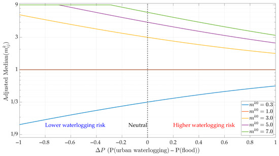
Figure 1.
Effect of evolutionary trend index on evaluation median .
4.4. Consensus Reaching Model Based on Decision-Makers’ Risk Preferences
4.4.1. Bounded Confidence Values Based on Decision Makers’ Risk Preferences
In SNGDM, DMs’ evaluation values typically reflect their risk preferences. Through interactions, DMs understand each other’s evaluation criteria, and identify relative risk levels by comparing evaluation values [35,46,47]. When a DM’s assessment differs significantly from others, decision pressure may arise. If a DM’s evaluation values exceeds that of neighboring nodes, they tend to affirm certain attributes of alternative options, maintain an optimistic view of the current state, and exhibit risk-seeking behavior [35]. Such DMs generally possess strong stress resilience, greater confidence in their judgments, and may overestimate their capabilities, leading to overreliance on personal assessments and reduced willingness to engage with others, thereby narrowing their interaction boundaries. Conversely, if a DM’s evaluation value is lower than those of neighbors, they tend to reject certain attributes of alternatives, adopt a pessimistic attitude, and demonstrate risk-averse tendencies. Risk-averse DMs are usually more cautious, have lower stress tolerance, and are more sensitive to reputational risks arising from divergence with majority opinions [48]. Consequently, they are more inclined to integrate others’ insights and revise their original evaluation values.
The individual risk preference of DM is quantified by the risk preference , which is defined as follows [35]:
When , DM is characterized as risk-averse; when , is risk-neutral; and when , exhibits risk-seeking behavior.
Reference [32] indicates that the BC value is influenced by both individual self-confidences [49] and the structure of the trust network. Building on this foundation, this study introduces a new formulation that explicitly incorporates the influence of risk preference. Specifically, a revised calculation method is proposed by integrating a risk preference to modify the traditional BC value. The resulting expression is presented in Equation (18):
where represents the BC value of DM for ; represents the risk sensitivity coefficient, satisfying ; and represents the trust degree of DM for . In addition, represents the self-confidence of DM , as shown below [32]:
In addition, if , then let ; if , then let .
When , the DMs exhibit risk-seeking behavior, characterized by strong stress tolerance, high confidence in personal evaluation values, and a tendency to adhere to initial judgments, thereby narrowing the interaction boundary. When , the DMs demonstrate risk-averse behavior, with lower stress tolerance and greater susceptibility to external influence, leading to an expanded reference boundary and a higher inclination to integrate others’ evaluation opinions. When , the DMs are risk-neutral; the BC value is minimally affected by external inputs, resulting in relatively stable evaluation values.
The effect of risk preference on the adjustment of the BC value will be further illustrated through a sensitivity analysis in Section 6.2.
4.4.2. Consensus Reaching Process
To enhance the efficiency and consistency of SNGDM, this study develops a two-stage consensus-reaching model comprising consensus level measurement and dynamic feedback adjustment. The specific process is as follows:
Stage 1: Consensus Measurement
To assess the consistency of group evaluation values, this study proposes a consensus measurement method tailored for TIFNs under Saaty’s nine-point scale. The process consists of three main steps: calculating individual consensus levels (ICLs), optimizing DMs’ weights, and evaluating the overall group consensus level (GCL).
First, the degree of divergence in evaluations among DMs is assessed by calculating the distance between their evaluation values. The distance between and is defined as follows [32]:
To eliminate the scale effect introduced by the Saaty nine-point scale [1/9,9], a normalization process is used to map the distances into the interval [0,1]. This ensures cross-scale comparability and consistency in subsequent calculations. The normalization procedure, newly proposed in this study, is described as follows:
Based on this, the ICL of DM can be obtained as follows [32]:
Secondly, to enhance the accuracy of consensus measurement and the authority of decision outcomes, it is essential to determine the DMs’ weights. To balance the subjective authority and the objective consistency of their evaluation values, this study adopts a hybrid weighting approach. Subjective weights are derived from the trust network, reflecting each DM’s competence and level of recognition within the group. Objective weights are calculated based on the similarity between individual DMs and the group as a whole. A novel DM weighting optimization model is then proposed to maximize both trust degree and similarity:
where represents the trust degree of DM ; represents the similarity between and ; and represents the overall similarity between and the group. The parameter is a preference adjustment coefficient that balances the influence of trust degree and similarity. Accordingly, the weight vector of DMs is defined as .
Finally, the weighted GCL is calculated based on each DM’s ICL and their corresponding weight, as follows [32]:
A GCL closer to 1 indicates a higher degree of consensus among the group. Given a predefined consensus threshold , if , consensus is considered achieved, and the group may proceed with the final decision. If , a feedback mechanism is activated to identify individuals whose evaluation values require adjustment in order to enhance the overall consensus level.
Stage 2: Dynamic Feedback Adjustment
To enhance group consensus, an iterative feedback model is established to dynamically adjust individual evaluation values when consensus has not been reached. The procedure includes the following steps:
Step 1: Adjustment of DMs’ Evaluation Values
Construct the set of DMs subject to the following constraints [26]:
where ensures that at least one DM accepts the adjustment proposal; represents the conflict degree between and in their trust relationship; represents the conflict threshold; and determines the final consensus level, while guarantees space for improvement and enhances the model’s efficiency.
A pair of DMs with the lowest similarity in the set is selected and adjusted as follows [32]:
where represents the feedback parameter, represents the adjusted evaluation value of DM , is the original evaluation value of , and represents the original evaluation value of .
Step 2: Iteration Termination Criterion
After each adjustment, the GCL is recalculated. If , consensus is considered to be reached, and the process proceeds to the alternative aggregation phase; otherwise, the iteration returns to Step 1 and continues until consensus is reached.
4.4.3. Alternative Selection
Step 1: Aggregate the evaluation values of all DMs as follows [32]:
where .
Step 2: Calculate the overall dominance score of alternative [40]:
Step 3: Rank the alternatives according to their scores, where a higher score indicates better performance. The highest-ranked alternative is identified as optimal. Formally, if , then , where ‘’ denotes ‘is superior to’.
4.4.4. Alternative Adjustment
After implementing the optimal alternative, the nodes are updated based on real-time observational data. The optimal alternative is incorporated into the BN as an input node, and the occurrence probabilities of the current disaster node and its subsequent node , denoted as and , are updated accordingly. Based on the evolutionary trend index of the flood disaster chain, the evolving trend is assessed to determine whether dynamic adjustment of the alternative is required:
If , the trend indicates deterioration, suggesting that the disaster is significantly evolving toward secondary hazards. Priority should be given to the risk of secondary disaster development, and relevant components of the original alternative should be adjusted accordingly.
If , the trend has eased, and the original alternative can continue without modification.
If , the disaster chain is at an unstable evolutionary threshold. Partial adjustments to the response measures may be necessary to enhance system resilience.
4.5. Steps of the Proposed Method
To enhance the dynamic adaptability of emergency alternatives for flood disaster chains, this study proposes an SNGDM method that integrates the evolutionary trends of flood disaster chains with DMs’ risk preferences. The specific steps are as follows:
Step 1: Construct the BN model of the flood disaster chain to identify causal pathways among primary and secondary disasters. Using literature-derived BN data and expert knowledge, input prior and conditional probabilities to infer the occurrence probabilities of disaster nodes at each stage.
Step 2: Calculate the evolutionary trend index from the inferred probabilities of disaster nodes and use this index to adjust the initial evaluation value of DMs.
Step 3: Calculate the risk preference of each DM using Equation (17), to determine the risk preference type, and compute the corresponding BC value using Equation (18).
Step 4: Compute the distances between DMs using Equations (20)–(21), and determine their weights using Equation (23). Then, calculate the GCL to assess whether consensus is reached. If consensus is reached, proceed to Step 6; otherwise, continue to Step 5 for iterative adjustment.
Step 5: Identify the DM pair with the maximum distance that satisfies the condition in Equation (25), and adjust their evaluation values according to Equation (26). Recalculate the GCL and repeat the adjustment process until the , then proceed to Step 6.
Step 6: Calculate the overall score for each alternative using Equations (27) and (28), and select the optimal alternative.
Step 7: After implementing the optimal alternative, update the BN based on the latest disaster node information. Recalculate the evolutionary trend index to determine whether further alternative adjustments are necessary.
The overall process of the proposed method is illustrated in Figure 2, and the stepwise procedure is provided in Appendix A.2, Algorithm A1.
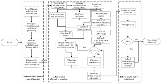
Figure 2.
SNGDM model for the flood disaster chain.
5. Case Study
5.1. Case Description
To verify the feasibility and effectiveness of the proposed method, a case study was conducted in Zhengzhou, Henan Province, China. Zhengzhou (112°42′–114°14′ E, 34°16′–34°58′ N) covers an area of approximately 1010 km2 and receives an average annual precipitation of 625.9 mm. Since 2006, the city has experienced over 15 heavy rainfall events each year, with economic losses per event exceeding 30 million USD [50]. In addition, the city serves as a major transportation hub, where frequent heavy rainfall often leads to waterlogging that disrupts traffic and causes severe cascading impacts.
This study draws upon the documented case of the “7.20” extraordinary rainstorm in Zhengzhou, Henan Province, China, with data obtained from [51]. The precipitation intensity during this event far exceeded historical averages within a short time frame, causing a rapid rise in river levels and extensive inundation across urban and peri-urban areas. The drainage system was quickly overwhelmed, leading to widespread urban waterlogging and severely disrupting the urban transportation network. In addition, communication and power supply systems were affected in several districts. This event exhibited a typical disaster chain evolution: flooding → urban waterlogging → road network disruption. Local authorities issued a red rainstorm warning on July 19 and escalated the emergency response to the highest level on 20 July. By 21 July, cumulative precipitation had reached 449 mm within 72 h. This period was selected for detailed analysis. Based on data in [51], the four emergency alternatives were redefined, and three additional attributes—on-site situation control , casualties and rescue conditions , and response speed —were incorporated to reflect the influence on decision-making. Evaluation data from five DMs representing the public security fire department, the medical department, and other relevant sectors, were used. As the literature evaluation values were expressed as pairwise comparisons of DMs’ preferences for alternatives, they were transformed into the median values of TIFNs represented using the 1–9 Saaty scale, supplemented with corresponding membership and non-membership degrees. The logical consistency of the TIFN matrices was verified by checking the reciprocal properties of all pairwise comparisons, confirming the stability and rationality of the DMs’ original judgments. Table 3 presents the initial evaluation values of DM , while Table 4 provides the corresponding trust matrix. The four alternatives are summarized as follows:
Table 3.
Initial decision matrix of DM . This table presents the initial pairwise comparison scores of four alternatives (–) under three criteria (–), as assessed by the DM . Each entry is expressed as a TIFN, including lower, middle, and upper bounds, along with membership and non-membership degrees.
Table 4.
Trust matrix of DMs. This table presents the trust degree between DMs and , with diagonal values of 1 indicating self-trust.
: Focuses on targeted search and rescue, real-time evacuation broadcasts, temporary flood barriers, staged urban drainage, and traffic control. Emphasizes on-site situation control () and rapid response ().
: Centers on centralized resettlement, water accumulation monitoring, rapid deployment of drainage teams, and dynamic public transportation adjustments. Highlights casualty reduction and rescue effectiveness () while supporting situational control ().
: Implements segmented rescue assisted by drones, designates emergency shelters, clears drainage pipelines, and manages traffic flow. Balances all criteria (–) to improve response coordination.
: Integrates rescue teams prioritizing vulnerable populations, tiered disaster response, cross-department resource allocation, and rapid restoration of infrastructure. Focuses on strategic control and system-wide rapid response ( and ).
Before conducting the decision-making analysis, the relevant parameters and assumptions are specified as follows:
- (1)
- Attributes. For simplicity, three attributes are considered with corresponding weights . In practice, the number of attributes may be much larger. The proposed method is thematically scalable, as BN construction, evaluation value modeling with TIFNs, and the consensus-reaching process impose no restriction on dimensionality. Although additional attributes increase computational load, efficiency can be maintained through dimensionality reduction or hierarchical evaluation.
- (2)
- DMs and trust network. This study considers a group of five DMs, assuming that this group size is sufficient to demonstrate the dynamics of the proposed model and the consensus-reaching process. It is further assumed that the trust network is complete—each DM can provide a trust degree for every other DM—and that these values remain constant throughout the consensus process. Under these assumptions, the consensus model is computationally efficient. While the method can be applied to larger groups, in practice, the trust network is likely to be sparse, requiring additional techniques to handle missing trust data, which represents an important avenue for future research.
- (3)
- BN. The BN nodes and their state classifications are defined according to standards from the China Meteorological Administration, geohazard engineering guidelines, and the relevant literature (Table 5). The BN probabilities are primarily derived from the BN established using seven years of historical flood and rainfall data in Zhengzhou [50], together with related BN analyses reported in [9], and are further supplemented with findings from other flood-related BN studies and expert knowledge to address incomplete records and obtain reliable probability estimates.
Table 5. BN nodes and state distributions of the flood disaster chain. This table presents the nodes of the flood disaster chain BN along with their corresponding state definitions and ranges, used to model disaster propagation and support decision analysis.
- (4)
- Parameter settings. Following relevant studies such as [25] and [32], the parameters are set as follows: adjustment threshold ; conflict threshold ; feedback parameter ; consensus threshold ; and preference adjustment coefficient between trust degree and similarity . In addition, the risk sensitivity coefficient is set to 0.5, with further analysis of this parameter provided in Section 6.1.
By explicitly stating these assumptions, the methodological robustness of the proposed approach is strengthened, and its applicability to complex real-world decision-making scenarios is clarified.
5.2. Application and Results
The selection procedure for the optimal alternative in this case is as follows:
Step 1: The BN model of the flood disaster chain was developed using GeNIe software, as illustrated in Figure 3.
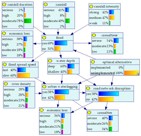
Figure 3.
BN of the flood disaster chain at the initial stage. Arrows indicate conditional dependencies between nodes.
It can be inferred that the initial probability of the flood event is , while the resulting probability of urban waterlogging is , yielding . It provides a crucial early warning of emerging waterlogging risks that static evaluations fail to capture.
Step 2: Based on the evolutionary trend index of the flood disaster chain, the initial decision matrix is adjusted according to Equation (16) and Table 2. An example of the adjusted decision matrix for DM is presented in Table 6.
Table 6.
Adjusted decision matrix of DM . This table presents the adjusted pairwise comparison scores of four alternatives (–) under three criteria (–), as assessed by the DM .
Step 3: Based on the adjusted decision matrix, the risk preferences of the DMs are calculated using Equation (17), resulting in , , , , .
Accordingly, the BC values for different risk preferences are presented in Table 7.
Table 7.
BC values of DMs. This table presents the pairwise BC values between DM and .
Step 4: The distances between DMs were calculated using Equations (20) and (21), as presented in Table 8.
Table 8.
Distances between DMs. This table presents the calculated distances between DM and , reflecting the degree of difference in their evaluation values.
Meanwhile, the DMs’ weights are calculated based on Equation (23) as follows: , , , , . According to Equations (22) and (24), the GCL is obtained as . Therefore, evaluation values need to be adjusted accordingly.
Step 5: As shown in Table 8, the distance between DMs and is the largest and satisfies condition (25); therefore, adjustment is performed according to Equation (26). After two iterations, , it is considered that consensus has been reached, and the iterative adjustment is terminated.
Step 6: Calculate the overall score of the alternatives, resulting in: , , , and . Therefore, is identified as the optimal alternative. Note that all variables involved in the calculations are defined in Appendix A Table A1.
Step 7: Following the implementation of the optimal alternative , the BN was updated based on the current disaster node information, as illustrated in Figure 4. At this stage, indicated that while alternative achieved partial control over the primary flood event, it failed to effectively interrupt the cascading progression toward urban waterlogging. Waterlogging subsequently became the main source of pressure in the ongoing emergency response. This finding is consistent with the situation observed during the 19 July Henan flood, where an insufficient response led to severe urban inundation on 20 July, thereby supporting the validity of the proposed model. At this point, the proposed method suggested timely adjustment of response strategies, which corresponds with the actual situation. To prevent further propagation of the flood disaster chain, alternative was strategically revised, resulting in an enhanced version, denoted as The key improvements introduced in include the following targeted measures: (1) diversion ditches and backflow gates to facilitate rapid drainage; (2) tiered scheduling in urban pump stations, with automatic frequency adjustment to rainfall intensity; (3) temporary retention areas and mobile drainage units supported by block-level monitoring; (4) distributed alarms and remotely controlled barriers to protect underground spaces (e.g., subways and underpasses); and (5) regular dissemination of flood warnings and evacuation routes through broadcasting systems and mobile applications.
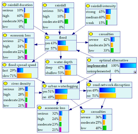
Figure 4.
Updated BN of the flood disaster chain. Arrows indicate conditional dependencies between nodes.
Through the above optimization, the response capacity to secondary disasters—specifically urban waterlogging—has been significantly enhanced. The proposed emergency alternatives align more closely with the evolving flood disaster chain, thereby improving the system’s dynamic adaptability and risk mitigation capability.
This case illustrates that static models maintain fixed evaluation values based on the initial flood conditions, whereas the proposed model dynamically incorporates the evolution of the flood disaster chain and updates the optimal alternative whenever the BN detects secondary risk escalation (), thereby enhancing decision adaptability and better capturing evolving disaster risks compared to static approaches. Moreover, considering that risk preferences affect BC values and thereby influence the number of iterations required during the consensus-reaching process, we conducted a detailed analysis of risk preferences based on the data in Table 7, as presented in Section 6.2.
6. Sensitivity and Comparative Analyses
6.1. Sensitivity Analysis of the Risk Adjustment Coefficient
To examine the impact of the risk adjustment coefficient on the BC value , a sensitivity analysis was conducted.
The DMs’ self-confidence and the trust degree were fixed at 0.75 and 0.6. The risk preference was varied across a set of representative values: [−1, −0.5, 0, 0.5, 1]. For each value of , was calculated over the entire range of with a step size of 0.01. The results are illustrated in Figure 5.
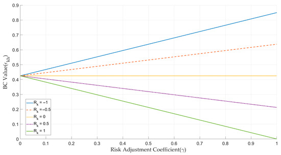
Figure 5.
Sensitivity of to across varying DMs’ risk preferences.
As shown in Figure 5, the influence of risk preference increases significantly with higher values. In particular, a clear divergence in emerges between risk-seeking and risk-averse DMs. The analysis indicates that when falls within the range , the variation in across the three types of DM remains relatively stable. This range preserves the differentiation in interaction willingness driven by risk preference, while avoiding excessive adjustment that could lead to information fragmentation among DMs.
Among these values, is identified as a representative optimal point. Located at the center of the stable interval, it offers a balanced compromise and demonstrates strong model stability. It guides convergence reasonably for risk-averse DMs, maintains the subjective influence of risk-seeking individuals, and proves applicable to a wide range of emergency response decision-making scenarios. Accordingly, is adopted as the default parameter in this study.
6.2. Sensitivity Analysis of Risk Preference
Equations (17)–(19) describe the effect of risk preference on the adjustment of the BC value . To illustrate this effect, we conducted a sensitivity analysis using the data in Table 7.
Figure 6 shows how variations in the risk preferences influence the BC values among the five DMs. Each curve represents a DM’s adjusted BC value toward others as the risk preference ranges from −1 to 1. The results show that risk-averse behavior increases BC values, whereas risk-seeking behavior decreases BC values.
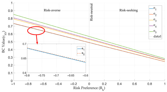
Figure 6.
Effect of risk preference on BC values .
In addition, Figure 7 and Figure 8 illustrate the influence of DMs’ risk preferences on BC values, taking (, risk-seeking), and (, risk-averse) as representative examples. Figure 7 compares DM ’s risk-adjusted BC values toward other DMs under four scenarios: extreme risk-seeking (), unadjusted (), extreme risk-averse (), and the actual observed value (). Figure 8 presents the same comparison for DM , with scenarios defined as . Note that when , the results correspond to the traditional BC model without risk adjustment. In contrast, under risk-seeking () and risk-averse () scenarios, the adaptive BC model produces different BC values, underscoring how risk attitudes reshape the consensus process, and highlighting the novelty of the proposed approach relative to traditional models.
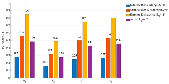
Figure 7.
Comparison of BC values for DM under different risk preferences .
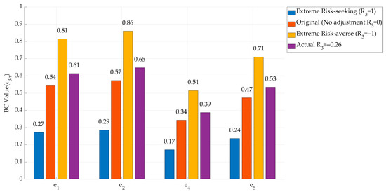
Figure 8.
Comparison of BC values for DM under different risk preferences .
In conclusion, the sensitivity analysis shows that DMs’ risk preferences influence BC values. Risk-averse DMs tend to enlarge BC values, indicating a greater willingness to accommodate others’ opinions; in contrast, risk-seeking DMs reduce BC values, reflecting a lower tolerance for differing opinions. Equation (25) further shows that variations in BC values determine the extent to which DMs must adjust their evaluations during the consensus-reaching process, thereby influencing the final consensus outcome.
6.3. Comparative Analysis
To validate the rationality and effectiveness of the proposed method, this study conducts a comparative analysis with existing approaches, focusing on two key aspects: the evolutionary trend of the flood disaster chain and the consensus-reaching process. The results are summarized in Table 9.
Table 9.
Comparison of different methods. This table summarizes the features and performance of existing and proposed methods.
(1) Comparison of methods for analyzing the evolutionary trends of flood disaster chains:
In analyzing the evolutionary trends of flood disaster chains, existing studies primarily utilize a BN to predict and verify the cascading paths of disasters and their potential losses. For example, Reference [9] employs a BN to identify critical nodes for emergency alternatives, focusing mainly on qualitative analysis. In contrast, this study advances the approach by introducing a quantitative analysis of the evolutionary trend through the construction of an evolutionary trend index. This enhancement provides stronger data support for subsequent decision-making processes and improves the overall decision-making capability of the model.
(2) Comparison of consensus reaching methods
Firstly, most existing studies on initial evaluation values adopt a static approach in SNGDM. For instance, Reference [29] uses precise numbers, while References [32,52] employ intuitionistic fuzzy numbers to represent evaluation values. However, these methods do not consider the dynamic changes of evaluation values during the evolution of flood disaster chains, limiting their applicability to the complex and rapidly changing characteristics of such scenarios. In contrast, this study introduces TIFNs to represent evaluation values and integrates the evolutionary trend index of the disaster chain to construct a dynamic evaluation values adjustment mechanism. This approach enhances the model’s ability to capture and respond to variations in DMs’ evaluation values under complex emergency contexts.
Secondly, regarding the BC model, this study proposes a dynamic BC framework that integrates self-confidence, trust networks, and risk preferences. Unlike Reference [29], which assumes a constant BC value; Reference [52], which considers only DMs’ self-confidence; and Reference [32], which incorporates both self-confidence and trust networks, this study further incorporates DMs’ risk preferences into the BC model. This enhancement improves the behavioral rationality of group evaluation coordination and increases the model’s adaptability.
Finally, as shown in Table 9, the numerical comparison indicates that although the proposed method required two iterations to reach convergence, this should not be viewed as a drawback. Rather, it is a natural outcome of incorporating richer behavioral mechanisms, including self-confidence, trust networks, and risk preferences. The additional iteration reflects a more realistic adjustment process in group decision-making rather than inefficiency. Importantly, all methods consistently converged to the same ranking order (), confirming that the proposed method enriches the decision-making process without compromising the validity of results.
7. Conclusions
The flood disaster chain, characterized by cascading effects, time-dependent uncertainty, and feedback-responsive dynamics, poses substantial challenges to traditional SNGDM methods. To address these challenges, this study proposes a novel SNGDM method that quantifies the evolutionary trends of flood disaster chains and incorporates BC value adjustments based on DMs’ risk preferences.
First, a BN is constructed to quantify the evolutionary trend of the flood disaster chain, enabling the dynamic adjustment of DMs’ evaluation values, which are represented by TIFNs. Based on these adjusted evaluations, DMs’ risk preference types are identified. Then, an adaptive BC model is developed by incorporating risk preferences, self-confidences, and the trust network to facilitate consensus formation among DMs. Furthermore, the optimal alternative is identified through weighted aggregation and embedded into the BN for iterative updates during implementation, allowing for real-time feedback and dynamic adjustment of the selected alternative. Finally, the superiority of the proposed method over static and risk-neutral models is clearly demonstrated through the case study of the flood disaster chain during the “7∙20” extreme rainfall in Zhengzhou, Henan Province, China, together with sensitivity and comparative analyses. The results show that risk-averse DMs tend to enlarge BC values, indicating greater willingness to accommodate others’ opinions, whereas risk-seeking DMs reduce BC values, reflecting lower tolerance for differing opinions and thereby resisting consensus. Moreover, in contrast to static models that maintain fixed evaluation values based on initial flood conditions, the proposed method dynamically integrates the evolution of the flood disaster chain and updates the optimal alternative whenever the BN detects secondary risk escalation. This dynamic adjustment not only enhances decision adaptability but also enables the model to better capture evolving disaster risks in complex emergency scenarios. Overall, the findings confirm that the proposed method effectively integrates dynamic disaster evolution with behavioral heterogeneity, thereby providing realistic and adaptive decision support in flood emergency management.
Despite these contributions, several limitations remain. The BN was constructed from expert knowledge and data reported in the literature, which provide empirical support but still introduce some subjectivity in node and probability specification. Moreover, the case study involved a relatively small group and a limited number of evaluation attributes, potentially limiting the generalizability of the findings. Future research could extend the model to larger groups, incorporate more diverse expert input and historical data, consider additional attributes, and develop automated BN learning methods and user-friendly decision-support tools to enhance practical applicability in complex disaster contexts.
Author Contributions
Formal analysis, R.M., L.Z., A.Z. and Y.W.; Funding acquisition, Z.W.; Visualization, R.M., L.Z., A.Z. and Y.W.; Writing—original draft, R.M. and Z.W.; Writing—review and editing, R.M. and Z.W. All authors have read and agreed to the published version of the manuscript.
Funding
This research was funded by the National Natural Science Foundation of China (Grant Nos. 72074002 and 71704001), the Natural Science Foundation of Anhui Province (Grant No. 2208085Y20), and the Foundation for Distinguished Young Scholars of Anhui Provincial Department of Education (Grant No. 2022AH020031).
Data Availability Statement
The original contributions presented in this study are included in the article. Further inquiries can be directed to the corresponding author.
Conflicts of Interest
The authors declare no conflicts of interest.
Appendix A
Appendix A.1. List of Abbreviations and Symbols
For clarity and ease of reference, all abbreviations and symbols used in this study are summarized in Table A1 to support understanding of the methodological framework and numerical analysis.
Table A1.
List of abbreviations and symbols.
Table A1.
List of abbreviations and symbols.
| Abbreviation/Symbols | Meanings |
|---|---|
| BN | Bayesian network |
| DM | Decision-maker |
| GDM | Group decision-making |
| SNGDM | Social network group decision-making |
| TIFNs | Triangular intuitionistic fuzzy numbers |
| BC | Bounded confidence |
| Trust matrix of DMs | |
| DMs set | |
| Alternative set | |
| Attributes set | |
| Attribute weights | |
| Decision matrix | |
| . | |
| Disaster events set | |
| Primary disaster | |
| Evolutionary trend index | |
| Initial evaluation values | |
| Adjusted median value | |
| ; | |
| Risk sensitivity coefficient | |
| ICL | Individual consensus levels |
| GCL | Group consensus level |
| Preference adjustment coefficient between trust degree and similarity | |
| Weight vector of DMs | |
| Consensus threshold | |
| Adjustment threshold | |
| Feedback parameter | |
| Conflict threshold |
Appendix A.2. Stepwise Algorithm of the Proposed SNGDM Method
Algorithm A1 presents a stepwise summary of the proposed SNGDM method for flood disaster chains, linking each computational step to Section 4.5 and illustrating the closed-loop process of prediction, decision, and feedback as shown in Figure 2.
| Algorithm A1. Proposed SNGDM method for flood disaster chains. |
| Input: BN nodes, Prior and conditional probabilities of the BN, Trust matrix , Decision matrix , Consensus threshold Output: Optimal alternative 1: Construct BN and infer disaster node occurrence probabilities 2: Compute evolutionary trend index and adjust evaluations based on 3: Calculate DMs’ risk preferences and BC values 4: Compute distances between DMs and weights 5: Calculate group consensus level while do Adjust evaluations of the DM pair with the maximum disagreement Recalculate end while 6: Aggregate evaluations and select provisional optimal alternative 7: Update BN and recalculate if > 0 then Adjust the alternative else if < 0 then Retain alternative unchanged else Partially adjust alternative to enhance resilience end if 8: return Optimal alternative |
References
- Balaian, S.K.; Sanders, B.F.; Abdolhosseini Qomi, M.J. How urban form impacts flooding. Nat. Commun. 2024, 15, 6911. [Google Scholar] [CrossRef]
- Wang, Y.M.; Ye, Z.J.; Jia, X.R.; Liu, H.F.; Zhou, G.Q.; Wang, L.B. Flood disaster chain deduction based on cascading failures in urban critical infrastructure. Reliab. Eng. Syst. Saf. 2025, 261, 111160. [Google Scholar] [CrossRef]
- Chen, Y.L.; Zhang, L.D.; Chen, X.H. A Framework for using event evolutionary graphs to rapidly assess the vulnerability of urban flood cascade compound disaster event networks. J. Hydrol. 2024, 642, 131783. [Google Scholar] [CrossRef]
- Top 10 International Natural Disaster Events in 2024. Available online: https://www.gddat.cn/gw/micro-file-simple/api/file/showFile/920804e8-0194-232a304c-001f-ff808081 (accessed on 25 June 2025).
- Lu, Y.M.; Qiao, S.T.; Yao, Y.R. Risk assessment of typhoon disaster chain based on knowledge graph and Bayesian network. Sustainability 2025, 17, 331. [Google Scholar] [CrossRef]
- AghaKouchak, A.; Huning, L.S.; Chiang, F.; Sadegh, M.; Vahedifard, F.; Mazdiyasni, O.; Moftakhari, H.; Mallakpour, I. How do natural hazards cascade to cause disasters? Nature 2018, 561, 458–460. [Google Scholar] [CrossRef] [PubMed]
- Zhao, Q.S.; Wang, J.D. Disaster chain scenarios evolutionary analysis and simulation based on fuzzy Petri net: A case study on marine oil spill disaster. IEEE Access 2019, 7, 183010–183023. [Google Scholar] [CrossRef]
- Wang, J.X.; Gu, X.Y.; Huang, T.R. Using Bayesian networks in analyzing powerful earthquake disaster chains. Nat. Hazards 2013, 68, 509–527. [Google Scholar] [CrossRef]
- Huang, L.D.; Chen, T.; Deng, Q.; Zhou, Y.L. Reasoning disaster chains with Bayesian network estimated under expert prior knowledge. Int. J. Disaster Risk Sci. 2023, 14, 1011–1028. [Google Scholar] [CrossRef]
- Guo, H.B.; Huang, C.; Zhang, C.X.; Shao, Q.L. A Novel comprehensive system for analyzing and evaluating storm surge disaster chains based on complex networks. Front. Mar. Sci. 2024, 11, 1510791. [Google Scholar] [CrossRef]
- Zhang, Y.H.; Fang, J.; Shen, D.T.; Yang, W.T.; Wang, X.L.; Lyu, L. Urban flood risk evaluation using social media data and Bayesian network approach: A spatial-temporal dynamic analysis in Wuhan city, China. Sust. Cities Soc. 2025, 126, 106388. [Google Scholar] [CrossRef]
- Mohammadi, S.; Bensi, M.T.; Kao, S.C.; DeNeale, S.T.; Kanney, J.; Yegorova, E.; Carr, M.L. Bayesian-motivated probabilistic model of hurricane-induced multimechanism flood hazards. J. Waterw. Port Coast. Ocean Eng. 2023, 149, 04023007. [Google Scholar] [CrossRef]
- Zhang, Y.X.; Hong, Y.; Guizani, M.; Wu, S.; Zhang, P.Y.; Liu, R.Q. A Multi-layer information dissemination model and interference optimization strategy for communication networks in disaster areas. IEEE Trans. Veh. Technol. 2024, 73, 1239–1252. [Google Scholar] [CrossRef]
- Lan, T.J.; Hu, Y.F.; Cheng, L.L.; Chen, L.W.; Guan, X.J.; Yang, Y.; Guo, Y.; Pan, J. Floods and diarrheal morbidity: Evidence on the relationship, effect modifiers, and attributable risk from Sichuan province, China. J. Glob. Health 2022, 12, 11007. [Google Scholar] [CrossRef]
- Zheng, Y.H.; Li, J.H.; Zhu, T.F.; Li, J.R. Experimental and MPM modelling of widened levee failure under the combined effect of heavy rainfall and high riverine water levels. Comput. Geotech. 2025, 184, 107259. [Google Scholar] [CrossRef]
- Huang, S.; Zhang, L.; Li, D. Research on simpliffied evaluation method for soil-rock mixed slope stability under dam-break flood impact. Bull. Eng. Geol. Environ. 2025, 84, 46. [Google Scholar] [CrossRef]
- Xu, Z.; Zhu, Y.; Fan, J.J.; Zhou, Q.; Gu, D.L.; Tian, Y. A spatiotemporal casualty assessment method caused by earthquake falling debris of building clusters considering human emergency behaviors. Int. J. Disaster Risk Reduct. 2025, 117, 105206. [Google Scholar] [CrossRef]
- Liu, G.Y.; Zhong, Z.R.; Ye, T.J.; Meng, J.; Zhao, S.Z.; Liu, J.J.; Luo, S.Y. Impact failure and disaster processes associated with rockfalls based on three-dimensional discontinuous deformation analysis. Earth Surf. Process. Landf. 2024, 49, 3344–3366. [Google Scholar] [CrossRef]
- Qin, Q.D.; Liang, F.Q.; Li, L.; Chen, Y.W.; Yu, G.F. A TODIM-based multi-criteria group decision making with triangular intuitionistic fuzzy numbers. Appl. Soft Comput. 2017, 55, 93–107. [Google Scholar] [CrossRef]
- Jiang, J.C.; Liu, X.-D.; Wang, Z.W.; Ding, W.P.; Zhang, S.T. Large group emergency decision-making with bi-directional trust in social networks: A probabilistic hesitant fuzzy integrated cloud approach. Inf. Fusion 2024, 102, 102062. [Google Scholar] [CrossRef]
- Yue, Q.; Deng, Z.B.; Hu, B.; Tao, Y.; Zou, W.C. Some novel theories of triangular intuitionistic fuzzy numbers and its application in two-sided matching. IEEE Access 2023, 11, 83461–83491. [Google Scholar] [CrossRef]
- Lu, Z.M.; Li, Y.T. A multi-criteria framework for sustainability evaluation of hydrogen-based multi-microgrid systems under triangular intuitionistic fuzzy environment. Sustainability 2023, 15, 3708. [Google Scholar] [CrossRef]
- Huang, C.; Wu, X.Y. Intuitionistic Fuzzy Method for Criteria Weights in MCGDM Based on Degree of Consensus. In Proceedings of the 2024 5th Information Communication Technologies Conference (ICTC), Ninjing, China, 10–12 May 2024; pp. 314–318. [Google Scholar]
- Shen, Y.F.; Ma, X.L.; Zhang, H.J.; Zhan, J.M. Fusion social network and regret theory for a consensus model with minority opinions in large-scale group decision making. Inf. Fusion 2024, 112, 102548. [Google Scholar] [CrossRef]
- Zhang, Y.J.J.; Chen, X.; Gao, L.; Dong, Y.C.; Witold, P. Consensus reaching with trust evolution in social network group decision making. Expert Syst. Appl. 2022, 188, 116022. [Google Scholar] [CrossRef]
- Li, Y.H.; Kou, G.; Li, G.X.; Peng, Y. Consensus reaching process in large-scale group decision making based on bounded confidence and social network. Eur. J. Oper. Res. 2022, 303, 790–802. [Google Scholar] [CrossRef]
- Yang, W.; Zhang, L.X.; Shi, J.R.; Lin, R.Y. New consensus reaching process with minimum adjustment and feedback mechanism for large-scale group decision making problems under social trust networks. Eng. Appl. Artif. Intell. 2024, 133, 108230. [Google Scholar] [CrossRef]
- Liang, X.; Guo, J.; Liu, P.D. A consensus model considers managing manipulative and overconfident behaviours in large-scale group decision-making. Inf. Sci. 2024, 654, 119848. [Google Scholar] [CrossRef]
- Zha, Q.B.; Dong, Y.C.; Chiclana, F.; Herrera-Viedma, E. Consensus reaching in multiple attribute group decision making: A multi-stage optimization feedback mechanism with individual bounded confidences. IEEE Trans. Fuzzy Syst. 2022, 30, 3333–3346. [Google Scholar] [CrossRef]
- Lu, X.Y.; Dong, J.Y.; Wan, S.P.; Li, H.C. The strategy of consensus and consistency improving considering bounded confidence for group interval-valued intuitionistic multiplicative best-worst method. Inf. Sci. 2024, 669, 120489. [Google Scholar] [CrossRef]
- Zhou, M.; Zheng, Y.Q.; Chen, Y.W.; Cheng, B.Y.; Enriue, H.V.; Wu, J. A large-scale group consensus reaching approach considering self-confidence with two-tuple linguistic trust/distrust relationship and its application in life cycle sustainability Assessment. Inf. Fusion 2023, 94, 181–199. [Google Scholar] [CrossRef]
- Liu, N.N.; Zhang, X.Z.; Wu, H.Y. A consensus-reaching model considering decision-makers’ willingness in social network-based large-scale group decision-making. Inf. Fusion 2025, 116, 102797. [Google Scholar] [CrossRef]
- Liang, D.C.; Wang, M.W.; Xu, Z.S.; Liu, D. Risk appetite dual hesitant fuzzy three-way decisions with TODIM. Inf. Sci. 2020, 507, 585–605. [Google Scholar] [CrossRef]
- Chen, T.; Wang, Y.T.; Wang, J.Q.; Li, L.; Cheng, P.F. Multistage decision framework for the selection of renewable energy sources Based on prospect theory and PROMETHEE. Int. J. Fuzzy Syst. 2020, 22, 1535–1551. [Google Scholar] [CrossRef]
- Sun, X.L.; Zhu, J.J.; Wang, J.P.; Perez-Galvez, I.J.; Cabrerizo, F.J. Consensus-reaching process in multi-stage large-Scale group decision-making based on social network analysis: Exploring the implication of herding behavior. Inf. Fusion 2024, 104, 102184. [Google Scholar] [CrossRef]
- Li, W.F.; Gao, J.W.; Mao, Y.C. An α-risk appetite cost minimizing model for multi-commodity capacitated p-hub median problem with time windows and uncertain flows. Ann. Oper. Res. 2024, 333, 79–121. [Google Scholar] [CrossRef]
- Gong, X.M.; Yu, C.R.; Min, L.Y. A cloud theory-based multi-objective portfolio selection model with variable risk appetite. Expert Syst. Appl. 2021, 176, 114911. [Google Scholar] [CrossRef]
- Li, D.F. A ratio ranking method of triangular intuitionistic fuzzy numbers and its application to MADM problems. Comput. Math. Appl. 2010, 60, 1557–1570. [Google Scholar] [CrossRef]
- Li, D.F. A note on “using intuitionistic fuzzy sets for fault-tree analysis on printed circuit board assembly”. Microelectron. Reliab. 2008, 48, 1741. [Google Scholar] [CrossRef]
- Wang, J.Q.; Nie, R.R.; Zhang, H.Y.; Chen, X.H. New operators on triangular intuitionistic fuzzy numbers and their applications in system fault analysis. Inf. Sci. 2013, 251, 79–95. [Google Scholar] [CrossRef]
- Wan, S.P.; Wang, Q.Y.; Dong, J.Y. The extended VIKOR method for multi-attribute group decision making with triangular intuitionistic fuzzy numbers. Knowl.-Based Syst. 2013, 52, 65–77. [Google Scholar] [CrossRef]
- Xie, X.; Huang, L.; Marson, S.M.; Wei, G. Emergency response process for sudden rainstorm and flooding: Scenario deduction and Bayesian network analysis using evidence theory and knowledge meta-theory. Nat. Hazards 2023, 117, 3307–3329. [Google Scholar] [CrossRef]
- Koller, D.; Friedman, N. Probabilistic Graphical Models: Principles and Techniques; Adaptive Computation and Machine Learning; MIT Press: Cambridge, MA, USA, 2010; ISBN 978-0-262-01319-2. [Google Scholar]
- Victor, P.; Cornelis, C.; Cock, M.D.; Teredesai, A.M. Trust- and distrust-based recommendations for controversial reviews. IEEE Intell. Syst. 2011, 26, 48–55. [Google Scholar] [CrossRef]
- Saaty, R.W. The analytic hierarchy process—What it is and how it is used. Math. Model. 1987, 9, 161–176. [Google Scholar] [CrossRef]
- Xu, X.H.; Yin, X.P.; Chen, X.H. A large-group emergency risk decision method based on data mining of public attribute preferences. Knowl.-Based Syst. 2019, 163, 495–509. [Google Scholar] [CrossRef]
- Gai, T.T.; Cao, M.S.; Chiclana, F.; Zhang, Z.; Dong, Y.C.; Herrera-Viedma, E.; Wu, J. Consensus-trust driven bidirectional feedback mechanism for improving consensus in social network large-group decision making. Group Decis. Negot. 2023, 32, 45–74. [Google Scholar] [CrossRef]
- Maug, E.; Naik, N. Herding and delegated portfolio management: The impact of relative performance evaluation on asset allocation. Q. J. Finance 2011, 1, 265–292. [Google Scholar] [CrossRef]
- Tan, J.J.; Wang, Y.M.; Chu, J.F. A consensus method in social network large-scale group decision making with interval information. Expert Syst. Appl. 2024, 237, 121560. [Google Scholar] [CrossRef]
- Wu, Z.; Shen, Y.X.; Wang, H.L.; Wu, M. Assessing urban flood disaster risk using Bayesian network model and GIS applications. Geomat. Nat. Hazards Risk 2019, 10, 2163–2184. [Google Scholar] [CrossRef]
- Liu, Z.; Wang, W.; Liu, P. Dynamic consensus of large group emergency decision-making under dual-trust relationship-based social network. Inf. Sci. 2022, 615, 58–89. [Google Scholar] [CrossRef]
- Yang, G.R.; Wang, X.Q.; Ding, R.X.; Lin, S.P.; Lou, Q.H.; Herrera-Viedma, E. Managing non-cooperative behaviors in large-scale group decision making based on trust relationships and confidence levels of decision makers. Inf. Fusion 2023, 97, 101820. [Google Scholar] [CrossRef]
Disclaimer/Publisher’s Note: The statements, opinions and data contained in all publications are solely those of the individual author(s) and contributor(s) and not of MDPI and/or the editor(s). MDPI and/or the editor(s) disclaim responsibility for any injury to people or property resulting from any ideas, methods, instructions or products referred to in the content. |
© 2025 by the authors. Licensee MDPI, Basel, Switzerland. This article is an open access article distributed under the terms and conditions of the Creative Commons Attribution (CC BY) license (https://creativecommons.org/licenses/by/4.0/).