Abstract
The paper presents a multigrid algorithm with the effective procedure for finding problem-dependent components of smoothers. The discrete Neumann-type boundary value problem is taken as a model problem. To overcome the difficulties caused by the singularity of the coefficient matrix of the resulting system of linear equations, the discrete Neumann-type boundary value problem is solved by direct Gauss elimination on the coarsest level. At finer grid levels, Lavrentiev (shift) regularization is used to construct the approximate solutions of singular or ill-conditioned problems. The regularization parameter for the unperturbed systems can be defined using the proximity of solutions obtained at the coarser grid levels. The paper presents the multigrid algorithm, an analysis of convergence and perturbation errors, a procedure for the definition of the starting guess for the Neumann boundary value problem satisfying the compatibility condition, and an extrapolation of solutions of regularized linear systems. This robust algorithm with the least number of problem-dependent components will be useful in solving the industrial problems.
Keywords:
singular and ill-conditioned systems; boundary value problems; Lavrentiev regularization; robust multigrid technique MSC:
65F10; 65F22; 65N55
1. Introduction
Let denote a discrete analogue of linear boundary value problem (BVP) with eliminated boundary conditions. The pure Neumann boundary conditions, which specify the normal derivative of a solution on the boundary, result in the singular coefficient matrix A. Three main properties can immediately be seen: (1) the determinant of a singular matrix is equal to zero; (2) its inverse () is not defined; and (3) a singular matrix always has at least one eigenvalue equal to zero. As a result, if a solution of exists, then it is not unique: any constant function is a solution of the homogeneous system: . This singular behavior of the coefficient matrix A has to be taken into account separately by any iterative solver [1,2,3,4,5,6].
The Neumann boundary value problem (NBVP) for the Poison equation has numerous applications in heat transfer, fluid dynamics, electrostatics, solid mechanics and other branches of physics and engineering. Currently, various numerical methods for solving the singular linear system have been proposed and developed [7]. One of them, the Lavrentiev regularization, adds a regularization term to the original system for transforming it into a well-posed problem [8]. The choice of the regularization parameter is critical for the success of the Lavrentiev regularization: a larger value leads to a more stable but potentially less accurate solution [9,10,11]. The advantages of this approach are that it is simple and that it does not affect the smoothing used in multigrid methods.
The Robust Multigrid Technique (RMT) had been developed for solving the industrial and real-life problems [12]. For the given purpose, the RMT has the following advantages:
- (1)
- Robustness: the only additional problem-dependent component (the number of smoothing iterations on coarse levels) compared to the single-grid smoothers;
- (2)
- Efficiency: close-to-optimal algorithmic complexity;
- (3)
- Almost full parallelism;
- (4)
- Low memory implementation.
The goal of this activity is to construct an effective procedure for finding problem-dependent components of iterative algorithms for black-box software. The numerical solution of a singular system arising from the discretization of the NBVP is chosen as a model problem. Practitioners often use the following procedure when solving industrial problems. Let
be a parameter-dependent problem, where is an under- (for example, pressure correction equation in the SIMPLE method) or overrelaxation parameter. The simplest iterative scheme for this parameter-dependent problem becomes
where is the iteration counter. If the parameter-dependent system is solved for different values starting from the same initial guess , then an empirical dependence can be constructed. The optimal value of minimizes the number of iterations: . The advantage of this procedure is its robustness: the optimal value can be determined without knowing the matrix spectrum. This procedure has the disadvantage that the computation of is the main fraction cost of the overall effort for solving the given parameter-dependent problem.
The RMT uses the independent systems
for (parallel) solving the discrete BVP, where zero level is the finest grid and is the coarsest level. The basic idea behind the RMT-based algorithm is that the discrete BVP can be solved by direct Gauss elimination on the coarsest level without regularization. After that, the regularized discrete BVPs are used for smoothing on the finer levels, and only a few iterations are needed for convergence. Since all computational grids of the same level are similar to each other, it is natural to assume that the optimal values of problem-dependent components will be approximately the same for all grids of the same level:
In other words, the optimal value can be found on one or several grids of the same level l, and the obtained value can be taken for all grids of the given level l. As a result, the amount of extra work on this level is negligible. This assumption is usually the most general one, and thus the results may be the strongest that can be obtained. The coarse level solution is a sufficiently accurate approximation to the fine level solution, and it used a priori information for determining the regularization parameter. On the finest grid (), the optimal value is computed by extrapolating the optimal values obtained at the other levels .
A similar procedure can be used to adapt the computational grid to the features of the numerical solution. Currently, there have been numerous attempts to improve the computational algorithms for BVP using the artificial intelligence-based technologies. The authors hope that the opportunities for the development of these computational algorithms are not yet completed and the solvers can be improved without artificial intelligence. Various problem-dependent strategies for finding the optimal value of the regularization parameter are given in [13,14,15,16] and others.
The article is organized as follows: first, some theoretical results on the iterative solution of regularized systems and 1D illustration are presented. After that, some theoretical estimations for a two-grid algorithm are given. In the Section 4, the RMT is used for solving a 3D NBVP, and further multigrid preconditioning as well as the extrapolation of the solution and choice of the initial guess for the iterative solver are both discussed.
The development of parallel and high-performance computational techniques for the mathematical simulation of physical and chemical processes will have an impressive influence on UN SDGs (Sustainable Development Goals: Clean Water and Sanitation, Affordable and Clean Energy, Industry, Innovation and Infrastructure, Climate Action, Sustainable Cities and Communities and others) as the United Nations’ chief initiative for advancing basic living standards and addressing a range of global issues.
2. Single-Grid Solver
Here, the Neumann boundary value problem (NBVP) for the Poisson equation
is considered in the unit cube , where g is a known function. If a solution of the boundary value problem exists, then it is not unique. The integration of (1) over the domain results in the following compatibility condition:
Solutions of the continuous boundary value problem (1) exist if (and only if) the compatibility condition is satisfied.
The standard seven-point discrete Laplacian on a square mesh with mesh size , where ℵ is a discretization parameter, becomes
where the function is a discrete analogue of u in (1).
The elimination of Neumann boundary conditions and lexicographic ordering of the unknowns make it possible to rewrite the discrete NBVP in matrix form
with a singular symmetric coefficient matrix A (all diagonal entries ). This means that and A is the non-invertible matrix (i.e., is not defined). Many real-life applications lead to the systems of algebraic equations with a singular () or ill-conditioned () coefficient matrix.
Together with (2), the regularized system
will be considered and analyzed, where I is an identity matrix and is a regularization parameter (Lavrentiev method, [8]). The regularized problem (3) is constructed in such a way that a major difficulty of the original problem (2) is overcome: the term shifts all eigenvalues of the coefficient matrix A on , so is the invertible matrix.
Let
denote the value of diagonal dominance in each row of the matrix A, and
Theorem 1.
For a diagonally dominant matrix A () with the positive diagonal () and the non-positive off-diagonal (, ) entries, the equality holds:
if .
It is possible to propose several iterative methods for solving the system (3), but Theorem 1 predicts that some of them will diverge:
Lemma 1.
The iterations
diverge for all in norm.
Proof of Lemma 1.
The iteration can be rewritten as follows:
where
is an iteration matrix. Since
If A is an invertible matrix and , then (5) becomes a direct solution algorithm.
Lemma 2.
The iterations
diverge for all in norm.
The main difficulty in the use of Lavrentiev regularization is the determination of . If (3) can be solved for , then we immediately have the solution . However, it is as difficult to solve (3) for as it is to solve (2) for . On the other hand, increasing the parameter results in the well-conditioned matrix with large solution error . In general, it is not possible to obtain a formula for the optimal value of the regularization parameter , but a robust approach for the adaptive Lavrentiev (shift) regularization will be proposed here.
To illustrate these remarks, consider the 1D NBVP
with exact solution , where C is some constant. The points
define a Cartesian uniform grid, where . The finite-difference analogue of becomes
The discrete Poisson equation with eliminated Neumann boundary conditions
- (1)
- (2)
- (3)
- can be written in the matrix form (3). In order to measure the convergence and accuracy of the numerical solution, the parameters are introduced as follows:
- (a)
- The relative residual normswhere is an approximation of the solution of (3) after iterations of the basic iterative or direct () method;
- (b)
- The error of the numerical solutionwhere .
First, we solve the 1D NBVP (6) in the matrix form (3) for different values of the regularization parameter by a direct (Thomas) algorithm (). Figure 1 represents convergence for sufficiently small if the coefficient matrix and the right-hand side vector are given exactly. In general, the divergence of the iterative/direct algorithm has to be expected for because A is the non-invertible matrix.
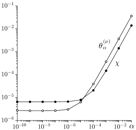
Figure 1.
The influence of the regularization parameter on the accuracy of the numerical solution of the 1D NBVP (6) ().
The strong influence of on the convergence rate of iterative methods is obvious. To illustrate what means, (7) should be rewritten as
The Gauss–Seidel iteration becomes
where is the iteration counter. The stopping criterion is defined as
Figure 2 demonstrates the required number of Gauss–Seidel iterations to reach this stopping criterion (11) for different starting . The following estimate holds
where is the exact solution of (7). In order to assess the numerical efficiency of an iterative solver, it is necessary to take into account the condition number . Because of Theorem 1 (4), the condition number becomes
It is easy to see that
and the estimation (12) becomes
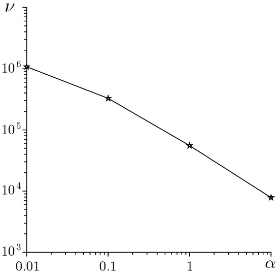
Figure 2.
The influence of the regularization parameter on the number of Gauss–Seidel iterations ().
The parameter in the stopping criterion can be roughly estimated as
i.e., the stopping criterion depends on . The regularization significantly increases the number of iterations required for sufficiently small ; i.e., the convergence rate of iterative algorithms deteriorates as (Figure 2).
For the NBVP (1), discretized on a uniform grid with mesh size h (2) and regularized by parameter , the smallest eigenvalue satisfies (3) and, for isotropic problems, it corresponds to just those eigenfunctions, which are very smooth geometrically in all spatial directions. On the other hand, the largest eigenvalue satisfies and corresponds to geometrically non-smooth eigenvectors. Here, and are the smallest and largest eigenvalues of matrix A (2), respectively.
In multigrid methods, the largest eigenvalue of the smoothing operator defines a reduction of the high-frequency errors in each smoothing step. Since , the Lavrentiev regularization does not affect the smoothing as shown in Figure 3. To highlight the smoothing effect of the Gauss–Seidel iterations, the initial guess is taken as an oscillating function
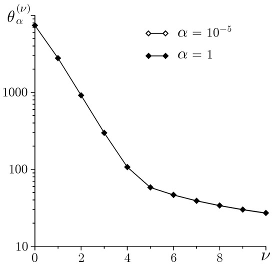
Figure 3.
Convergence during the first Gauss–Seidel iterations ().
As a result, h-independent convergence of the multigrid algorithm is expected as (Figure 4).
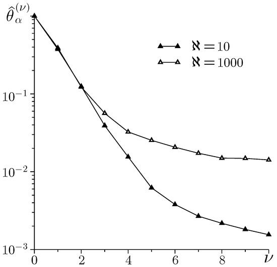
Figure 4.
h-independent convergence during the first Gauss–Seidel iterations ().
The development of robust multigrid solvers for singular and ill-conditioned discrete boundary value problems is a new challenge for scientific computing. Equation (3) can be rewritten as
Assuming a good estimate for and a stopping criterion
are given in advance, the parameter of regularization becomes
After that, the regularized system (3) can be solved by well-known multigrid methods. The main difficulty of this approach is a sufficiently accurate a priori estimation of the solution norm . In order to overcome this difficulty, the idea is to exploit the proximity of the solution of a discrete BVP obtained at adjacent grid levels of the Robust Multigrid Technique (RMT) [12].
3. The Two-Grid Algorithm
The simplest multigrid algorithm uses two grids: a fine grid and a coarse grid. The iteration formula of the multigrid methods reads
here, is the coarse grid correction after smoothing iterations on the fine grid, q is the multigrid iteration counter, and are the approximations to the solution before and after the qth multigrid iteration, respectively. The subscript <<0>> denotes an affiliation to the fine grid. The multiplication by matrix and subtraction of the right-hand vector result in
Assuming that the correction will be given is
where is some matrix, one multigrid step is of the form
After q multigrid steps, the equation becomes
A straightforward computation yields an estimate of the form
where
is the average reduction factor of the residual after q multigrid iterations. Then, it is necessary to determine the matrix and estimate the norm .
For completely consistent smoothers, the resulting equation reads
where
is the exact solution of a defect equation, is the smoothing iteration counter and is the smoothing iteration matrix. The starting guess for smoothing on the fine grid is an exact coarse grid solution
prolongated to the fine grid
where and are the restriction and prolongation operators, respectively. The subscript <<1>> denotes affiliation to the coarse grid.
The classical multigrid convergence analysis is based on two propositions [18]:
- (1)
- Smoothing property: existence of a monotonically decreasing function , such that for and
- (2)
- Approximation property: existence of a constant independent of such that
Here, for a singular matrix A and for an invertible matrix A. The smoothing and approximation properties should be proved for each case.
If the smoothing and approximation properties hold, then the estimation of the matrix (20) becomes
The h-independent convergence of multigrid iterations
is expected after a sufficient number of smoothing iterations on the finest grid.
The numerical solution of ill-conditioned industrial problems requires an analysis of the computational errors expressed as perturbations on the coefficient matrix and vectors of the resulting linear system. The perturbated defect equations on the fine and coarse grids becomes
where the perturbations of corrections and are caused by perturbations of the coefficient matrices and as well as the right-hand side vectors and . These equations result in the estimation
An elementary transformation of equations leads to the error estimation
where is the condition number of the coefficient matrix . First, let all perturbations of the coefficient matrix be zero ( and )
and the approximation property holds
In this case, fast convergence of the multigrid solver is expected. On the other hand, if perturbation of the right-hand side vector is zero () and the approximation property holds, then the estimation can be rewritten as
The rough estimation predicts that for each perturbed problem, there is an optimal value of the regularization parameter , so .
The Lavrentiev method for the regularization of linear ill-posed problems with noisy data had been studied by many researchers. A set of the parameter choice rules, which give good results also in the case of noise levels under- or overestimated many times, had been proposed [19,20].
4. Robust Multigrid Technique
In the late 1980s, the multigrid methods based on a multiple coarse grid correction strategy were proposed and developed. P. O. Frederickson and O. A. McBryan studied the efficiency of the Parallel Superconvergent Multigrid Method (PSMG); the basic idea behind the PSMG is that the even and odd points of the fine grid form two coarse grids [21,22]. The Robust Multigrid Technique (RMT) had been developed for advanced black-box software for the numerical simulation of physical and chemical processes by solving a “robustness–efficiency–parallelism” problem [12]. The RMT has the least number of problem-dependent components, full parallelism and close-to-optimal algorithmic complexity in low memory implementation. Figure 5 represents the triple coarsening used in the RMT: three coarse grids , and are generated by the agglomeration of the finite volumes on the fine grid . The finer and coarse grids in the RMT have these properties:
- 1.
- All coarse grids , and have no common grid points:
- 2.
- The finest grid can be represented as a union of the coarse grids , and :
- 3.
- All grids are geometrically similar, but the mesh size of the coarse grids , and is three times larger than the mesh size of the finest grid ;
- 4.
- Independently of the grid functions assignment, each finite volume on the coarse grids , and is a union of three finite volumes on the fine grid .

Figure 5.
The finest () and three coarse grids (, and ).
The classical multigrid methods use two types of coarsening: vertex-centred coarsening consists of deleting every other vertex in each direction, and cell-centred coarsening consists of taking unions of fine grid cells to obtain coarse grid cells. The triple coarsening uses both deleting vertex and finite volume agglomeration. The basic idea of triple coarsening is to agglomerate neighbour finite volumes with the selected one. As a result, each coarse volume consists of fine volumes independently on the grid function assignment to grid points (Figure 6). In combination with the additive property of definite integral, the triple coarsening results in an accurate finite volume discretization of BVPs on the multigrid structures. All coefficients of PDEs and the right-hand side function are discretized only on the finest grid (the so-called composite formula). Theoretical analysis shows l-independent accuracy of the definite integral evaluation on the multigrid structure [12]. This is a very important property for industrial problems, where some coefficients of PDEs may have the boundary layers or be highly oscillating functions. Such features make it difficult to evaluate these coefficients of discrete BVPs on the coarse grids of classical multigrid methods.
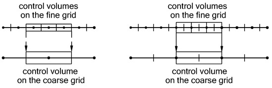
Figure 6.
The triple coarsening in the RMT: vertex • and volume face + (left) and vertex + and volume face • (right).
The RMT uses the most powerful coarse grid correction strategy where the most modes are approximated on the coarse grids in order to make the task of the smoother the least demanding.
The finest grid forms a zero grid level, but the coarse grids , and form the first grid level. The following triple coarsening is carried out recursively: each grid of level l is considered to be the finest grid for three coarse grids of level . Nine coarser grids obtained from three coarse grids of the first level form a second level. The grid hierarchy is called a multigrid structure () generated by the grid :
where is the number of the coarsest level. Each grid generates its own multigrid structure .
Let , and denote the exact solution of system (discrete BVP) and solutions of systems and obtained on levels l and , respectively. For second-order discretization, the estimation holds
where h is the mesh size of the finest grid, . The triangle inequality allows us to estimate the difference between the solutions and as follows:
This means that the solution obtained on the coarse level approximates the solution obtained on fine level l well. The discussion of convergence, stability, error analysis and parallelization of the RMT is given in numerous papers and summarized in [12].
For clarity, a 1D problem on the four-level multigrid structure () shown in Figure 7 is considered for an illustration of the algorithm. The multigrid iteration of the RMT starts on the coarsest level (Figure 8), where a direct method should be used for solving the discrete NBVP (2)
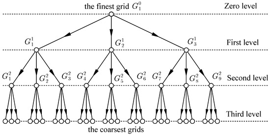
Figure 7.
The multigrid structure , .
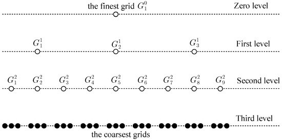
Figure 8.
Numerical solution of (22) by direct method on the coarsest level (•).
The numerical solution prolongated to the finer level becomes the starting guess
where is the problem-independent prolongation operator of the RMT [12]. Figure 9 and Figure 10 illustrate the problem-independent prolongation of the RMT.
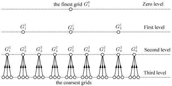
Figure 9.
Prolongation from the coarsest level.
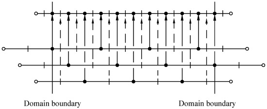
Figure 10.
The problem-independent prolongation in the RMT.
The resulting discrete problem that has to be solved on all grids of level is
where
After a few iteration steps
the error becomes smooth, where is the smoothing iteration counter and is a splitting matrix. In multigrid methods, it is assumed that the smoother is a convergent iterative method, i.e.,
The obtained function is the first multigrid iteration value , i.e.,
After that, the stopping criterion
is checked and, if necessary, the next multigrid iteration is performed or transferred to the fine grid. The substitution of in (23) gives
where is some residue. Adding a correction to the approximation to the solution of (23) required to eliminate the residue results in the defect equation
This equation on the coarsest level becomes
where is the problem-independent restriction operator of the RMT (Figure 11). After the solution of this defect equation, the correction should be prolongated to the fine level:
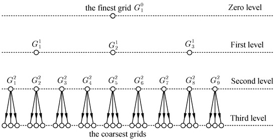
Figure 11.
Restriction from level .
After a few iteration steps (24) starting with the initial guess
the error becomes smooth and small, and a new approximation to the solution after second multigrid iteration is
The multigrid schedule of the RMT is the V-cycle with no pre-smoothing (a sawtooth cycle) with the dynamic finest grid, as shown in Figure 12 [12].
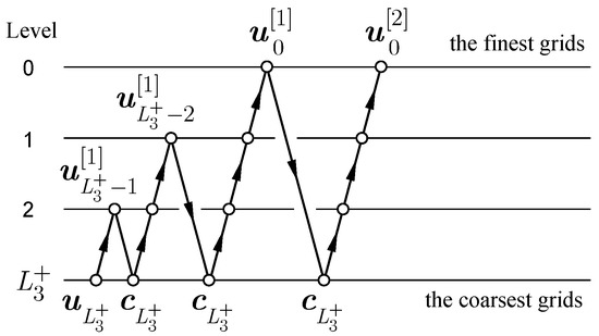
Figure 12.
Multigrid cycle of the RMT with two multigrid iteration on each level.
Since each coarse level consists of independent (without common points) and almost identical grids (Figure 5), all unknown problem-dependent parameters of the algorithm (for example, the number of smoothing iterations, under- and over-relaxation or regularization parameters, and others) can be found on one or several grids to achieve the fastest convergence rate or the highest accuracy possible, starting computations from the same initial guess [12]. The obtained pseudo-optimal value of the problem-dependent components is taken to be the same for all grids of the same level. In general, each coarse level l consists of grids, , , so the additional effort to optimize the RMT on one or several grids is negligible. This approach based on numerical experiments makes it possible to effectively optimize the RMT in solving real-life problems.
The NBVP (1) with the exact solution is used as a benchmark problem. Substitution of the exact solution into (1) gives the right-hand side function and the corresponding boundary conditions on faces of the unit cube . Figure 13 demonstrates the convergence of the RMT during five multigrid iterations () starting the iterant zero on (, ) and (, ) with the point Gauss–Seidel smoother and
- (1)
- The criterion of accuracy (15):
- (2)
- The regularization parameter (16) on the finer levels:
- (3)
- The level stopping criterion (11):
The error of the numerical solution (10) is computed on the finest grid after each multigrid iteration.
The multigrid cycle shown on Figure 12 makes it difficult to compare the convergence rate of the RMT if the multigrid structures have different numbers of levels. However, it is easy to see that the number of multigrid iterations q needed for solving (3) is approximately the same; i.e., h-independent convergence has been achieved.

Figure 13.
Convergence of the RMT after q multigrid iterations.
5. Multigrid Preconditioning
In the process of solving applied problems, it is often necessary to change the order or type of approximation of (initial-) boundary value problems and/or the computational grid to adapt to the features of the solution. For clarity, let us consider a linear boundary value problem
Here, and is a given open bounded domain with boundary , is a linear (elliptic) differential operator on and represents one or several linear boundary operators on , denotes a given function on and represents one or several functions on , is a solution, .
The generation of computational grid in the domain and some approximation (FDM, FVM, FEM, DG or others) of the BVP (25), some ordering of the unknowns and elimination of the boundary conditions allows us to rewrite the discrete analogue of (25) in matrix form
Within an arbitrary iterative process for the solution of a given discrete problem, the solution becomes
However, this approach is not always convenient: if it is necessary to increase the order of approximation of the BVP (25) on , then a significant part of the computer code will have to be rewritten. In general, it is more convenient to solve not the original system (26) but to use the defect correction approach and the auxiliary space method [18,23]. Let the high-order approximation of the BVP (25) on an unstructured grid in matrix form be (26). An body-unfitted Cartesian grid (auxiliary space) can be generated in the domain , and the discrete analogue of the BVP (25) on can be written in matrix form
The unstructured body-fitted grid makes it possible to obtain a more accurate approximation of the BVP (25), but on the other hand, the auxiliary structured grid allows us to construct a highly efficient (geometric multigrid) algorithm for solving systems of (non-)linear algebraic equations. The basic idea is to exploit the advantages of and with small change in computer code.
The system of linear equations should be rewritten as
there is a correction, is a residual computed on the unstructured grid , is a restriction operator transferring the residual from the unstructured grid to the structured grid (auxiliary space), and q is the intergrid iteration counter.
The two-grid algorithm can be represented as:
- (1)
- Computation of the residual on the unstructured grid ;
- (2)
- Restriction of the residual from the unstructured grid to the structured grid (auxiliary space), i.e., computation of the right-hand side of (28) ;
- (3)
- Solution of (28) by a geometric multigrid on the structured grid (auxiliary space)
- (4)
- Prolongation of the correction from the structured grid (auxiliary space) to the unstructured grid , i.e., computation of ;
- (5)
- Computation of the starting guess for the smoothing iterations
- (6)
- Smoothing on the unstructured gridwhere is a splitting matrix and is the smoothing iteration counter;
- (7)
- Computation of a new approximation to the solution (27)
The above-mentioned two-grid algorithm can be represented in matrix form
where is the smoothing iteration matrix. If the smoothing and approximation properties hold, then the h-independent convergence of the integrid iteration is expected (21).
Another problem is the definition of problem-dependent components of the algorithm (under- and over-relaxation parameters, regularization parameter, the number of smoothing iterations, etc.). All problem-dependent components can be determined experimentally, starting computations from the same initial guess. In practice, such an approach is justified when solving a series of systems with different right-hand sides: , . Since all grids of each level of a multigrid structure are similar to each other, determination of the problem-dependent components of the algorithm is possible on one or several grids of each level. The obtained pseudo-optimal values are taken to be the same for all grids of the same level. Theoretical analysis shows that this approach leads to an increase in the total execution time by several percent compared to the case when all problem-dependent components are known in advance. Figure 14 represents a generalization of the multigrid cycle shown in Figure 12 to the two-grid (structured–unstructured grids) algorithm.
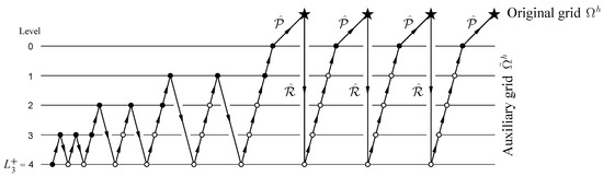
Figure 14.
Multigrid preconditioning: original (★) and auxiliary (∘) grids.
Another problem is the generation of the adaptive grids. In practice, the computational grids are often (locally or globally) refined, and the effect of grid refinement on the numerical solution is investigated for optimal adaptation of the grid to a numerical solution. MLAT is an example of local refinement of the structured grids [18]. The iterative process of the structured grid refinement can be formalized on the multigrid structure. Thus, after the first multigrid iteration on a structured grid , an approximation to the solution on an unstructured grid and a priori information about the unstructured grid (the density of vertices in the region ) are obtained. The procedure for rebuilding the auxiliary grid into the adaptive grid to simplify the intergrid operators and is presented in [12]. An FAS approach allows using the multigrid cycle shown in Figure 14 for solving the nonlinear BVP [12].
Thus, the combination of defect correction, auxiliary space and the adaptive determination of problem-dependent components of the algorithm by means of numerical experiments on one or several grids of each level starting from the same initial guess (except for the finest grid, where all problem-dependent components are determined by extrapolation from coarse levels) allows solving a wide class of problems in a unified way. The FAS method allows us to generalize this approach to the nonlinear case.
6. Extrapolation of the Solution
The extrapolation can be used to improve the accuracy of the solution of the regularized system (3). Let
be two linear system with a singular matrix A (2) and different regularization parameters and , where . A linear combination of (29a) multiplied by and (29b) multiplied by becomes
where
is the extrapolated solution and is some parameter chosen for minimization of the right-hand side of (30). The basic idea is to minimize the residual by an optimal choice of using the Euclidean scalar product
The right-hand side of (31) can be represented as
The second derivative of the function
predicts a single minimum of the function :
It is easy to see that
Obviously, for . Employing the extrapolation is one way to obtain more accurate approximations to the solution of singular system (2) in the sense of minimum .
7. Choice of Initial Guess for Iterative Solver
As a rule, the zero approximation to the solution of BVPs is used as a starting guess in the iterative processes. The NBVP (1) with the exact solution , the right-hand side function and the corresponding boundary conditions are used to illustrate a more accurate definition of the starting guess. The integration of (1) over squares leads to a variant of the compatibility condition:
or
Taking into account the Neumann boundary conditions,
this equation becomes
The exact integration simplifies the expression
The basic assumption is to represent the unknown solution as a sum of three one-dimensional functions , and :
After substitution of the representation (33) into (32), Equation (32) becomes an ordinary differential equation (ODE)
The boundary conditions are treated in the same manner, for example
Finally, a one-dimensional auxiliary NBVP
has the exact solution
Similarly, the functions and in (33) can be determined in the same way. The resulted starting guess is
For obvious reasons, it is necessary to compare the zero () and improved (35) starting guesses:
- (a)
- The difference between exact solution () and zero starting guess () in point () is
- (b)
- The difference between the exact solution () and the starting guess (35) in point () is
The above-mentioned approach makes it possible to obtain a starting guess to the solution of the NBVP that is more accurate than the zero one.
This simple algorithm is summarized as follows:
- (1)
- (2)
- (3)
- (4)
- Formation of the initial guess as (33).
8. Conclusions
An efficient multigrid algorithm for solving the singular or ill-conditioned discrete boundary value problems can be constructed on the basis of a direct solver on the coarsest levels and an iterative smoother of the regularized system on the fine levels.
The main results can be summarized as follows:
- (1)
- (2)
- (3)
- For perturbed singular or ill-conditioned systems, the regularization parameter must satisfy the condition ;
- (4)
- The Lavrentiev regularization does not affect the smoothing, and h-independent convergence of the multigrid algorithm is expected;
- (5)
- The regularization parameter in multigrid algorithms can be defined using the proximity of solutions obtained at the coarser grid levels;
- (6)
- A numerical solution of the regularized system with different parameters can be improved by extrapolation;
- (7)
- Representation (33) makes it possible to formulate a more accurate starting guess for BVPs than the zero one.
The proposed RMT-based procedures can be used for the adaptive determination of the problem-dependent components of the multigrid algorithm and adaptation of the computational grid to the features of the numerical solution in black-box software. The advantages of this approach are its simplicity of implementation, negligible additional efforts and robustness based on analysis of the experimental convergence rate.
Author Contributions
Conceptualization, methodology, software S.I.M.; formal analysis, review and editing, A.Y.V. All authors have read and agreed to the published version of the manuscript.
Funding
This work was supported by the Ministry of Science and Higher Education of the Russian Federation (State Assignment No. 075-00269-25-00).
Data Availability Statement
The original contributions presented in this study are included in the article. Further inquiries can be directed to the corresponding author.
Conflicts of Interest
The authors declare no conflicts of interest.
References
- Trottenberg, U.; Oosterlee, C.W.; Schüller, A. Multigrid; Academic Press: London, UK, 2000. [Google Scholar]
- Liao, Z.; Hayami, K.; Morikuni, K.; Yin, J.F. A stabilized GMRES method for singular and severely ill-conditioned systems of linear equations. Jpn. J. Ind. Appl. Math. 2022, 39, 717–751. [Google Scholar] [CrossRef]
- Yu, X.; Ma, C. The modified Uzawa methods for solving singular linear systems. Comput. Math. Appl. 2021, 104, 71–86. [Google Scholar] [CrossRef]
- Wang, M.; Bertsekas, D.P. On the Convergence of Simulation-based Iterative Methods for Solving Singular Linear Systems. Stoch. Syst. 2017, 3, 38–95. [Google Scholar] [CrossRef]
- Hong, L.Y.; Zhang, N. On the preconditioned MINRES method for solving singular linear systems. Comput. Appl. Math. 2022, 41, 304. [Google Scholar] [CrossRef]
- Eldén, L.; Simoncini, V. Solving Ill-Posed Linear Systems with GMRES and a Singular Preconditioner. SIAM J. Matrix Anal. Appl. 2012, 33, 1369–1394. [Google Scholar] [CrossRef]
- Buzhabadi, R. New Algorithms for Solving Singular Linear System. Comput. Math. Model. 2018, 29, 71–82. [Google Scholar] [CrossRef]
- Lavrentiev, M.M. Some Improperly Posed Problems of Mathematical Physics; Springer-Verlag: New York, NY, USA, 1967. [Google Scholar]
- Sheela, S.; Singh, A. Lavrentiev regularization of a singularly perturbed elliptic PDE. Appl. Math. Comput. 2004, 148, 189–205. [Google Scholar] [CrossRef]
- Morigi, S.; Reichel, L.; Sgallari, F. An iterative Lavrentiev regularization method. BIT Numer. Math. 2006, 46, 589–606. [Google Scholar] [CrossRef]
- Morozov, V.; Mukhamadiev, E.M.; Nazimov, A.B. Regularization of singular systems of linear algebraic equations by shifts. Comput. Math. Math. Phys. 2007, 47, 1885–1892. [Google Scholar] [CrossRef]
- Martynenko, S.I. Numerical Methods for Black-Box Software in Computational Continuum Mechanics; De Gruyter: Berlin, Germany, 2023. [Google Scholar] [CrossRef]
- Kaltenbacher, B. On the regularizing properties of a full multigrid method for ill-posed problems. Inverse Probl. 2001, 17, 767–788. [Google Scholar] [CrossRef]
- Zeng, C.; Luo, X.; Yang, S.; Li, F. A parameter choice strategy for a multilevel augmentation method in iterated Lavrentiev regularization. J. Inverse Ill-Posed Probl. 2018, 26, 153–170. [Google Scholar] [CrossRef]
- George, S.; Padikkal, J.; Remesh, K.; Argyros, M. A New Parameter Choice Strategy for Lavrentiev Regularization Method for Nonlinear Ill-Posed Equations. Mathematics 2022, 10, 3365. [Google Scholar] [CrossRef]
- Plato, R.; Mathé, P.; Hofmann, B.M. Optimal rates for Lavrentiev regularization with adjoint source conditions. Math. Comput. 2016, 87, 785–801. [Google Scholar] [CrossRef]
- Volkov, Y.S.; Miroshnichenko, V.L. Norm estimates for the inverses of matrices of monotone type and totally positive matrices. Sib. Math. J. 2009, 50, 982–987. [Google Scholar] [CrossRef]
- Hackbusch, W. Multi-Grid Methods and Applications; Springer: Berlin/Heidelberg, Germany, 1985. [Google Scholar]
- Raus, T.; Hämarik, U. On numerical realization of quasioptimal parameter choices in (iterated) Tikhonov and Lavrentiev regularization. Math. Model. Anal. 2009, 14, 99–108. [Google Scholar] [CrossRef][Green Version]
- Hämarik, U.; Palm, R.; Raus, T.A. A family of rules for the choice of the regularization parameter in the Lavrentiev method in the case of rough estimate of the noise level of the data. J. Inverse Ill-Posed Probl. 2012, 20, 831–854. [Google Scholar] [CrossRef]
- Frederickson, P.O.; McBryan, O.A. Parallel superconvergent multigrid. In Multigrid Methods: Theory, Applications and Supercomputing; McCormick, S., Ed.; Marcel Dekker: New York, NY, USA, 1988; pp. 195–210. [Google Scholar]
- Decker, N.H. Note on the Parallel Efficiency of the Frederickson-McBryan Multigrid Algorithm. SIAM J. Sci. Stat. Comput. 2005, 12, 208–220. [Google Scholar] [CrossRef]
- Xu, J. The auxiliary space method and optimal multigrid preconditioning techniques for unstructured grids. Computing 1996, 56, 215–235. [Google Scholar] [CrossRef]
Disclaimer/Publisher’s Note: The statements, opinions and data contained in all publications are solely those of the individual author(s) and contributor(s) and not of MDPI and/or the editor(s). MDPI and/or the editor(s) disclaim responsibility for any injury to people or property resulting from any ideas, methods, instructions or products referred to in the content. |
© 2025 by the authors. Licensee MDPI, Basel, Switzerland. This article is an open access article distributed under the terms and conditions of the Creative Commons Attribution (CC BY) license (https://creativecommons.org/licenses/by/4.0/).