Abstract
To address the challenge of effective roof support in fully mechanized excavation roadways, this paper proposes an adaptive control method for the initial support force of self-shifting temporary supports based on pressure sensors. First, the mechanical characteristics of the roof in fully mechanized excavation faces were analyzed, a static model of the roadway roof thin plate was established, the mechanical criteria for heading support were determined, and the reasonable calculation of the initial support force and working resistance for heading support was completed. Then, the pressure-control system of the hydraulic cylinder was modeled, achieving real-time online adjustment of PID control parameters based on fuzzy neural network control, and an adaptive control system for initial support force based on feedback from pressure sensors inside the hydraulic cylinder was constructed. Finally, comparative experiments of fuzzy neural network PID (FNN-PID) and fuzzy PID control were conducted in both the AMESim 2304 and Matlab/Simulink 2016 co-simulation environment and real physical scenarios. The effectiveness and advancement of the proposed control algorithm were verified.
Keywords:
fully mechanized excavation roadway; heading support; initial support force regulation; pressure feedback; fuzzy neural network MSC:
93C85
1. Introduction
As a core component of the global energy structure, coal accounts for over 40% of total electricity generation [1]. With the depletion of shallow resources, coal mining depths generally exceed 800 m, significantly increasing the risk of roof instability in roadway excavation under complex geological conditions. According to statistics from the China Academy of Mine Safety Technology, roof accidents account for 23% of all coal-mine accidents, and precise regulation of the initial support force of temporary support brackets is key to preventing such accidents [2]. The insufficient initial support force fails to effectively support the roadway roof, accelerating roof separation and shear failure; excessive initial support force can easily trigger “compression flow failure,” leading to roof fragmentation, hydraulic system overload, and potential accidents. Therefore, accurate calculation and control of the support force for temporary brackets in fully mechanized excavation faces are particularly critical [3].
Significant progress has been made in temporary support for current excavation operations across multiple research areas. In terms of equipment structure optimization, Liu et al. [4] developed a support-roof coupling mechanical model to improve self-shifting support design and Ding et al. [5] developed deep roadway supports with a height range of 275–380 cm, significantly enhancing positioning efficiency during support movement. Regarding support-force calculation models, international conventional methods (such as the UK’s WELSON method and Germany’s EVANS model) are based on static empirical formulas (e.g., the UK requires initial support intensity ≥75 times the mining height and support intensity ≥150 times the mining height and Germany specifies a minimum support intensity of 80 times the mining height) [6]; Wang Guofa et al. [7] established fundamental tenets for differential-strength coupled support systems and transient roadway bracing, advocating ‘minimal initiation force combined with elevated operational resistance. This approach significantly bolsters the resilience of provisional reinforcement mechanisms within high-stress environments susceptible to dynamic impacts. Cheng Jingyi et al. [8] constructed an intelligent perception model for support-roof interaction based on electro-hydraulic control big data, achieving roof-pressure prediction and roof-fall warning; Zhao Huimeng et al. [9] established a coupling dynamic model for advanced support equipment and surrounding rock, verifying its control effect on roof deformation; and Prof. Peng Syd S [10] from the U.S. optimized the temporary support working resistance calculation by introducing an additional force coefficient through geomechanical analysis. In research on temporary support-force control methods, Hu Xiangpeng et al. [11] employed the BP neural network PID to regulate initial support force; Xue Guanghui et al. [12] combined FLAC3D simulation with the neural network PID for adaptive tracking of surrounding rock pressure; and Li Yang [13] further enhanced dynamic response capability by integrating particle swarm optimization with the BP neural network (PSO-BP-PID). However, hydraulic-parameter disturbances in field applications result in >10% force control errors.
Furthermore, advanced adaptive control strategies have emerged in broader mechatronic systems. For example, neural network-based dynamic surface controllers achieve asymptotic tracking for hydraulic manipulators under model uncertainties, while novel output-feedback methods handle actuator deadzones/faults in Euler–Lagrange systems without velocity measurements. However, these approaches lack integration with geomechanical constraints specific to mining-support scenarios [14,15].
The limitations of the above research are the mechanical model lacks a real-time pressure-feedback mechanism, making it difficult to dynamically adjust the initial support force; the strong nonlinearity of the electro-hydraulic system causes traditional control responses to lag (error > 10%); and existing intelligent algorithms fail to simultaneously address roof load fluctuations and hydraulic parameter drift. To address this, this paper proposes an adaptive control method for the initial support force of self-shifting temporary supports based on pressure-sensor feedback. The innovations include, first, establishing a static thin-plate mechanics model of the roadway roof to derive mechanical criteria for roof stability, combined with real-time cavity pressure monitoring to construct a dynamic correction mechanism for initial support force; second, designing a fuzzy neural network PID (FNN-PID) algorithm that integrates the nonlinear adaptability of fuzzy logic with the self-learning characteristics of neural networks to optimize PID parameters online; and finally, through AMESim/Matlab co-simulation and underground testing, achieving a reduction in initial support-force tracking error from >10% to <±3.5%, with a 40% improvement in step-load response speed.
The value of this study lies in establishing an initial support-force calculation model to obtain roadway-adapted support forces, avoiding roof separation or compression damage caused by improper initial support; at the control efficiency level, reducing support-force adjustment time to 2.1 s achieves efficient adaptive control of temporary support forces. The paper’s structure is as follows: Section 2 and Section 3 analyzes roof mechanical properties and derives the initial support-force calculation model; Section 4 designs the FNN-PID controller; Section 5 verifies algorithm performance through co-simulation; Section 6 conducts underground engineering tests; and Section 7 summarizes research conclusions.
2. Analysis of Mechanical Behavior in Fully Mechanized Roadway Roofs
2.1. Working Scenario of Fully Mechanized Roadway
The tunneling construction of coal-mine roadways mainly includes slot cutting, coal cutting and falling, and coal loading and transportation. Each construction technology requires manual sequential operations to ensure continuity, with the construction process shown in Figure 1. The boom-type roadheader performs coal-breaking operations, cooperating with the bridge-type transfer machine and mine belt conveyor to complete the ‘three-transport’ process of coal production.
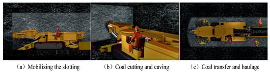
Figure 1.
Tunneling construction process of coal-mine roadways.
Subsequently, at the heading position of the roadway, self-shifting roadway supports are used for temporary support in fully mechanized tunneling. The self-shifting temporary support is powered by high-pressure oil from the variable pump on the crawler-mounted support vehicle, providing heading support within the roadway space. The crawler-mounted support vehicle is used in conjunction with the self-shifting temporary support, and its roof beam is designed with a chain transmission mechanism to assist in the positioning and movement of the self-shifting temporary support, thereby completing the support construction of the fully mechanized roadway. The spatial relationship between the self-shifting temporary support, crawler-mounted support vehicle, and boom-type roadheader in the fully mechanized roadway is shown in Figure 2, with the main technical characteristics listed in Table 1.
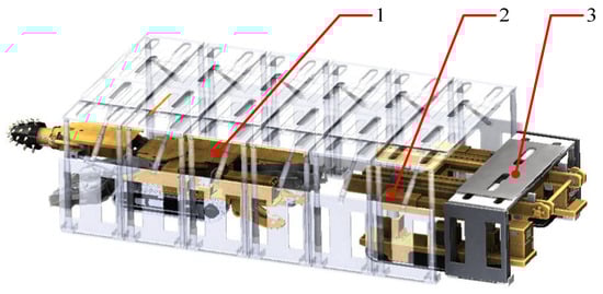
Figure 2.
Default view of the different devices in the fully mechanized roadway (1—boom-type roadheader, 2—crawler-mounted support vehicle, 3—self-shifting temporary support).

Table 1.
The main technical characteristics of self-shifting advanced support equipment.
The self-shifting temporary support mainly consists of four major components: load-bearing structural members, control elements, actuating elements, and auxiliary reset devices, as shown in Figure 3a. The load-bearing structural members include the roof beam, which directly contacts the roadway roof and bears the load; the side guard telescopic beam, hinged to the roof beam via a pushing jack to adjust support width; the sliding shoe base, which contacts the floor and transfers load; and the rib protection plate, which stabilizes the ribs, prevents rock entry, and withstands horizontal thrust. The actuating elements are support columns (located between the roof beam and base, bearing load and adjusting height), pushing jacks (connecting the roof beam and side guard beam), and balance jacks (connecting the side guard beam and rib protection plate). Control elements in the hydraulic system include safety valves, hydraulic control check valves, and control valves. The auxiliary reset device counters tilting under lateral forces, restores the support columns to a vertical position, and resists horizontal pressure.
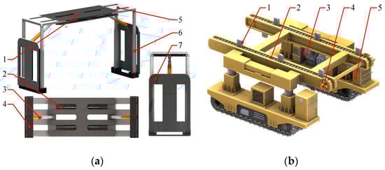
Figure 3.
Structural schematic diagram of the self-shifting advanced support unit. (a) Structural schematic diagram of the self-shifting temporary support (1—roof beam, 2—pushing jack, 3—balance jack, 4—sliding shoe base, 5—side-guard telescopic beam, 6—support column, 7—rib protection plate); (b) structural schematic diagram of the crawler-type support vehicle (1—wedge pushing block, 2—drive chain, 3—pump station and oil tank assembly, 4—sprocket, 5— control console).
The crawler-type support vehicle, shown in Figure 3b, is a tracked transport vehicle primarily composed of a transport mechanism, walking drive mechanism, hydraulic system, electrical system, water system, and lubrication system. Its tracked drive mechanism provides obstacle-crossing capability. A chain drive system (drive chains, sprockets, and wedge blocks) on the vehicle’s roof beam undertakes the transportation and relocation of the self-shifting temporary support. It carries the support to the working face end, using the rotation of the drive chains to complete transport and positioning, enabling rapid roadway heading support installation.
2.2. Fracture Characteristics of Roadway Roof
As excavation advances, it disrupts the original stress state of the surrounding rock, altering overlying strata stress. Depending on geology, this can cause stress concentration leading to roadway displacement or roof failure. The authors of Reference [16] identify four primary roof failure modes (which may occur concurrently), posing safety hazards:
- (1)
- Shear failure (Figure 4a): this occurs when roof deformation exceeds the rock’s ultimate shear strength. Causes include low inter-layer strength or high compressive stress at roof corners, generating significant local shear stress. This leads to upward-propagating fractures and shear-off;
- (2)
- Tensile failure (Figure 4b): this happens when deformation-induced tensile stress exceeds the rock’s ultimate tensile strength. Interconnected tensile failure surfaces can cause roof rock to slide along fractures;
- (3)
- Delamination and flexural failure (Figure 4c): this is a complete rupture from bending-induced tensile failure, common in roofs with weak interlayers. Joint surfaces oblique to maximum principal stress cause layer slippage and instability;
- (4)
- Compression-flow failure (Figure 4d): this is roof compression resulting from the above failures. Fractures initiate in the roof, floor, and corners, expanding inward to form a network, ultimately causing roof collapse.

Figure 4.
Structural schematic diagram of the self-shifting advanced support unit. (a) Shear failure. (b) Tensile failure. (c) Delamination and flexural failure. (d) Compression-flow failure.
2.3. Static Mechanical Model of Roadway Face Roof
To prevent the aforementioned roof-fracturing phenomena during roadway excavation, face support is required for the roadway. Simultaneously, to achieve effective support in fully mechanized excavation roadways, a static mechanical model and analysis of the face roof should first be conducted. This section employs an elastic plate model, which closely resembles the properties of the face roof in fully mechanized excavation roadways, for static analysis of the face roof, providing a foundational model for the subsequent rational calculation of initial support forces.
To facilitate simplified analysis, the following assumptions are made:
- (1)
- The rib sides, coal mass ahead of the face, and support operations behind the roadway provide certain support forces to the roof of the unsupported area, allowing the boundary of the roadway roof to be simplified as a fixed boundary;
- (2)
- The surrounding rock has a short exposure time, and the roof maintains good integrity, enabling the roof of the unsupported area to be treated as a continuous homogeneous medium;
- (3)
- The ratio of the roof thickness in the unsupported area to the roadway span satisfies the thin-plate condition, permitting the modeling of the roof in the unsupported area based on the thin-plate mechanical model.
Figure 5 shows a simplified schematic of the structural form of the excavation roadway space. The unsupported area of the immediate roof is located ahead of the area to be excavated, with the roadway sides on both sides, while the rear of the unsupported area is the permanent anchored zone supported by bolts and mesh. The boundary conditions of the roadway roof are “three edges fixed and one edge simply supported.” Thus, the boundary conditions for the fixed edges OA, OC, and BC are
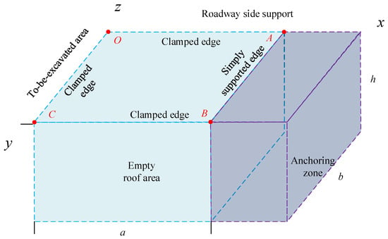
Figure 5.
The roof model of roadway head.
The boundary condition for the simply supported edge AB is
In the equation, ω(x,y) is the deflection function of the roof.
Typically, the thickness of the coal seam is less than 1/5 of the roadway width, satisfying the basic conditions of the thin plate model. The roof is subjected to a uniformly distributed load from the overlying rock layers in the vertical direction. The roof load can be decomposed into two components: one is the transverse load perpendicular to the mid-plane of the roof, and the other is the longitudinal load acting within the mid-plane of the roof. Below, a static thin plate model is established with which to discuss the stress, strain, and displacement issues caused by transverse loads.
According to the small deflection theory of elastic thin plates, two assumptions are first proposed for the elastic thin plate model:
- (1)
- Neglecting the smaller normal strain εz perpendicular to the central plane of the roadway, the line perpendicular to the central plane before and after roadway deformation always remains perpendicular to the central plane of the roadway;
- (2)
- The bending stresses σx, σy and torsional stresses τxy, τxz, τyz on the cross-section caused by a certain load are the main stresses generated, while the normal stress σz parallel to the mid-plane and the bending-torsional stresses are relatively small and can be neglected.
According to thin plate theory, the equilibrium equation of the roadway roof under external load q(x,y) is
where Mx, My, and Mxy are the bending moment components, in N·m, calculated as
where σx, σy, and σz are stress components; D is the bending stiffness of the roadway roof, D = Ez3/(12 − 12μ2) in N/m; E is the elastic modulus of the roof in MPa; and μ is the Poisson’s ratio.
Based on the above static model of the roof, the mechanical criterion for roof stability can be derived, providing a theoretical basis for the calculation of initial support force.
3. Calculation of Initial Support Force Based on Surrounding Rock Stability
3.1. Mechanical Criterion for Roadway Face Support
According to thin plate theory, during face support, the roadway roof is subjected to the external load q(x,y) from the overlying rock layers and the supporting force Fi from the self-shifting temporary support. The deflection differential equation of the roadway roof can be expressed as
Based on the boundary conditions of the roadway roof with ‘three edges fixed and one edge simply supported,’ the tensile stresses along the x and y axes can be obtained from the static model of the roof as
Meanwhile, according to Equation (4), substituting Mx and My, the tensile stresses σx and σy can be expressed in terms of the deflection equation ω as
Equation (7) indicates that the deformation of the roadway roof is not only related to factors such as the geological properties and geometric dimensions of the roof strata but is also influenced by the external load from the surrounding rock and the supporting force. Therefore, to maintain the stability of the roadway roof during excavation, hydraulic support equipment must provide timely support for the unsupported span, supplying appropriate supporting force to prevent fracturing and delamination at the roadway face. Thus, the effective support criterion for the roadway roof is σxmax < [ση], σymax < [ση].
3.2. Determination of Working Resistance for Roof Stability
Based on the above mechanical criterion for preventing roof fracturing, hydraulic support equipment must provide a certain working resistance during roadway support to ensure continuous roof stability and prevent the tensile stress of the roadway roof from exceeding its tensile stress limit. Using the static model of the roof and the expressions for tensile stresses σx and σy established in the previous section, the following can be derived:
In the equation, , where q represents the stress on the roof, and a and b denote the length and width of the roadway, respectively.
According to Equation (8), taking the tensile stress at the plane z = −h/2 (i.e., the bottom surface of the roof) as the study object, the maximum tensile stresses of the roof in the x and y directions are, respectively,
Based on the mechanical criterion for preventing roof fracture (σxmax < [ση]), substituting Q into the formula for σxmax yields Equation (10).
Equation (10) can be expressed as
Within the mathematical formulation, q denotes roof stress, quantified as the net stress distribution arising from the superposition of support forces and the overlying rock load P, expressed as
In the equation, P is the rock load of the roadway roof, kN; Fe is the working resistance of the hydraulic support equipment, kN.
Substituting Equation (12) into Equation (11) yields the hydraulic support resistance required to maintain tunnel stability:
At this point, during the face-support process of the roadway, to avoid excessive working resistance causing crushing and fracturing of the roadway roof, it is necessary to ensure that the working resistance meets the requirements for maintaining the stability of the surrounding rock roof.
3.3. Initial Support-Force Setting for Face Support
The initial support force of hydraulic support equipment is interrelated with the working resistance. A higher initial support force for face support enables the support to provide timely reinforcement to the roadway face roof, quickly achieving a stable working state and avoiding early delamination of the roadway face roof, which plays a positive role in maintaining the stability of the roadway roof. However, excessively high initial support force may lead to “squeeze-flow failure” in the roadway roof, placing undue burden on hydraulic components and oil pumps. Therefore, the initial support force for face support is typically calculated based on relevant empirical formulas:
In the formula, F0 is the initial support force at the face, kN; ρ is the setting coefficient of the initial support force, ρ ∈ [0.65, 0.8].
4. Initial Support-Force Regulation System Based on Pressure Feedback
The initial support-force regulation system based on pressure feedback first requires the construction of a pressure-control system model for the hydraulic cylinder of the support column. Subsequently, a hydraulic pressure-regulated modulation framework is implemented. This system utilizes chamber pressure measurements as its feedback signal, where the optimal initial supporting force required for roadway rock stability serves as the reference input. Through continuous real-time sampling of hydraulic actuator lower compartment pressures via the feedback circuit, the control unit dynamically adjusts outputs to maintain alignment with targeted pressure magnitudes. This meets the demand for different initial support forces in the parallel rapid excavation process of self-shifting temporary supports, completing the construction of an adaptive regulation method for the initial support force of self-shifting temporary supports.
4.1. Modeling of the Hydraulic Cylinder Pressure Control System for Support Columns
As the core equipment in the face-support process of fully mechanized excavation roadways, self-shifting temporary supports can provide reasonable initial support force to the roadway roof, preventing early delamination of the roadway face roof during excavation. During the face-support process, the four sets of hydraulic cylinders of the self-shifting temporary support lift the roof beam upward to achieve effective support for the roadway face roof.
The pressure control system of the hydraulic cylinder for the self-shifting temporary support mainly consists of key components such as the hydraulic cylinder, hydraulic control check valve, proportional relief valve, safety valve, and fixed-displacement hydraulic pump. The schematic diagram of the pressure control system for the column hydraulic cylinder is shown in Figure 6.
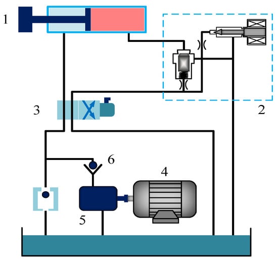
Figure 6.
Schematic diagram of the pressure control system of the column hydraulic cylinder (1—hydraulic cylinder, 2—proportional relief valve, 3—solenoid directional valve, 4—hydraulic motor, 5—hydraulic pump, 6—hydraulic control check valve).
Hydraulic System Modeling Approach (Figure 6): The hydraulic control check valve prevents pressure loss in the column hydraulic cylinders during face support, while the safety valve limits system pressure by opening at a preset threshold. Mathematical modeling and analysis focus on critical system components to determine relevant parameters for the hydraulic cylinder pressure control model.
Modeling simplifies the self-shifting temporary support system based on its characteristics. Key assumptions and priorities include
- (1)
- Omitting functional components like the hydraulic control check valve and proportional directional valve;
- (2)
- Prioritizing pressure control modeling for the lifting action of the column hydraulic cylinders; the lowering action is omitted;
- (3)
- Assuming all four column hydraulic cylinders contact the roadway roof simultaneously after spatial pose leveling;
- (4)
- Neglecting pressure losses in short hydraulic pipelines and avoiding complex fluid mass/dynamic effects;
- (5)
- Setting the hydraulic oil temperature as constant.
Practical applicability: Assumptions (1)–(2) prioritize core pressure control. Assumption (3) holds for flat roofs after leveling; minor irregularities are compensated by controller robustness (Section 4.1). Assumption (4) is valid for compact hydraulic circuits (typical of mining equipment), while (5) applies to short-term operations. High-fidelity co-simulation (Section 5) and field tests (Section 6) validate the model under realistic conditions.
- (1)
- Proportional Relief Valve Modeling
Currently, major manufacturers of large-scale mining hydraulic equipment widely recognize Bosch Rexroth proportional relief valves as highly reliable. Therefore, this paper selects the Bosch Rexroth pilot-operated electro-hydraulic proportional relief valve, which mainly consists of an electro-pilot valve and a main valve. The structure of some components is shown in Figure 7.
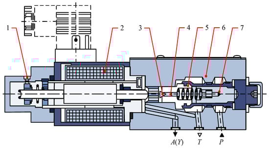
Figure 7.
The structure diagram of the pilot-controlled electro-hydraulic proportional valve (1—screw, 2—proportional solenoid, 3—pilot cone valve, 4—throttle, 5—valve assembly, 6—valve body, 7—valve spool).
Below, mathematical modeling of the proportional relief valve will be conducted, and based on its working principle, its mathematical model will be reasonably simplified and analyzed.
The proportional amplifier performs signal conditioning, computational processing, and power amplification on incoming voltage inputs. This transformed output current subsequently drives proportional solenoid valve operation. The frequency response of the proportional amplifier during operation is generally high and exceeds the cutoff frequency of other components in the system; thus it is simplified as a proportional element:
Kpa is the gain coefficient of the proportional amplifier, A/V; I(s) is the input current of the proportional amplifier during operation, A; and U(s) is the input voltage of the proportional amplifier during operation, V.
Upon energization of the proportional electromagnet, electromagnetic forces act upon the armature assembly. This mechanical displacement subsequently adjusts the pilot cone valve position, thereby modifying the cracking pressure threshold of the pilot stage. The frequency response of the proportional solenoid during operation is generally high, so it is also equivalently treated as a proportional element:
where Kps is the current-to-force gain coefficient of the proportional solenoid, N/A; F(s) is the output thrust generated by the solenoid on the pilot cone valve when current flows, N.
In the pilot-operated proportional relief valve, the armature directly contacts the pilot cone valve. When analyzing the force on the pilot valve spool, the command force on the cone valve can be equated to the thrust generated by the armature, yielding the mechanical equilibrium equation for the pilot valve spool:
where P4 is the outlet pressure of the pilot valve, N/m3; A4 is the effective acting area of the pilot valve spool, m2; P4A4 is the algebraic sum of hydraulic forces on the effective acting area, N; msp is the mass of the pilot valve spool, kg; x is the displacement of the spool, m; Bs is the equivalent damping coefficient of the valve, N/(m·s−1); Kes is the equivalent spring stiffness, N/m, which is the sum of mechanical spring stiffness and steady-state flow force stiffness; Fss1 is the steady-state flow force, N; and Fcf is the Coulomb friction force on the spool, N.
In the hydraulic-system environment, the values of P4A4, Fss1, and Fcf are relatively small. The simplification omitting P4A4, Fss1, and Fcf is justified by their minimal impact in mining hydraulic systems. P4A4 (hydraulic force) is orders smaller than dominant solenoid/spring forces due to low pilot-stage pressures. Fss1 (flow force) is mitigated through pressure-balanced valve design and absorbed in Kes. Fcf (friction) is insignificant versus viscous damping in lubricated spools. This aligns with Assumptions 4–5 (Section 4.1) and enables tractable linear modeling for core dynamics. Higher-order effects are inherently captured in AMESim co-simulation (Section 5).
Following standard mathematical conditioning procedures including variable reduction and Laplace domain conversion, the servo-valve core displacement response to electromagnetic excitation is derived as
By analyzing the force on the main valve spool, its mechanical equilibrium equation is obtained:
where P1 is the pressure at the lower end of the main valve, N/m2; A1 is the force-bearing area at the lower end of the main valve, m2; P2 is the pressure at the upper end of the main valve, N/m2; A2 is the force-bearing area at the upper end of the main valve, m2; y is the displacement of the spool, m; Δy is the pre-compression of the spring, m; and Fss2 is the steady-state flow force on the spool, N. The simplified linearized equation for Fss2 is Fss2 = Kfyy + KfpP1, where: Kfy = əFss2/əy, Kfp = əFss2/əP1; msm msm is the mass of the spool, kg; and Kss is the equivalent spring stiffness acting on the spool, N/m.
Rearranging and combining Equation (19), and performing Laplace transformation yields
Analyzing the flow at the hydraulic bridge, the flow equation can be obtained:
where Q2 is the flow rate toward pipeline R2, m3/s; Q1 is the flow rate toward pipeline R1, m3/s; Q1 = G1(P1 − P3), where G1 is the hydraulic conductance of the pipeline and P3 is the pressure at point A of the hydraulic bridge, N/m2; Q3 is the flow rate of the pipeline, m3/s, Q3 = Kspx + KsqpP4; Ksp is the flow gain of the pilot valve port; Ksqp is the pressure-flow coefficient of the pilot valve port; βe is the bulk modulus of elasticity of the main valve chamber, MPa; and V2 is the volume of the upper chamber of the main valve, m3.
Performing Laplace transformation on Equation (21) and substituting Q1 and Q3 yields
When supplied by a constant pressure source or with minimal pressure variation, ΔP3 = ΔP2 = ΔP4. By combining Equations (20) and (22), the expression for the main valve spool displacement y is obtained as
where ωrm is the natural frequency of the main valve, Hz; , ωrc is the corner frequency of the upper chamber of the main valve, Hz; and , ωrv is the corner frequency during the movement of the main valve spool, Hz; ; ; .
When the proportional relief valve is operational, the natural frequency ωrm of the main valve is typically much higher than other components, thus terms with high-frequency ωrm as the denominator in the expression can be omitted for simplification. The corner frequency ωrc of the main valve upper chamber is also generally at a high frequency, so terms with ωrc as the denominator can similarly be omitted. The frequency ωrA is usually small and close to the operating frequency of the main valve spool. The corner frequency ωrv primarily reflects the influence of the pilot hydraulic bridge on the speed of the main valve movement. Additionally, the expression for the main valve spool displacement shows that different effective working areas A will also affect the dynamic response of the main valve to some extent.
Based on the above analysis, Equation (23) can be simplified to
Meanwhile, the flow continuity equation for the pilot hydraulic bridge chamber is
In the equation, Q4 is the flow rate of the main valve’s lower chamber cavity, m3/s; V1 is the volume of the main valve’s lower chamber, m3; and Qsm is the flow rate through the main valve orifice, m3/s. The linearized equation for Qsm is: Qsm = KQfy + KQpP1, where KQf is the main valve flow gain, and KQp is the main valve pressure-flow coefficient.
Performing Laplace transform on Equation (23) yields
Combining Equations (24) and (26) and eliminating the intermediate variable y, the expression for the controlled parameter P1 in terms of the pilot valve spool displacement x and the disturbance Q4 is obtained as
In the equation, ; ; ; ; ; .
Utilizing the mathematical formulations presented in Equations (15), (17), (18) and (27), the cascaded configuration of component transfer functions yields the pilot proportional relief valve’s mathematical representation, illustrated graphically in Figure 8.
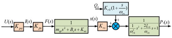
Figure 8.
Mathematical representation of the pilot-operated proportional relief valve system dynamics through cascaded transfer function connections.
The expression for the output pressure of the pilot proportional relief valve is
- (2)
- Hydraulic Cylinder Modeling
During the initial lifting and supporting process of the support-column hydraulic cylinder, the hydraulic cylinder lifts the roof beam of the support to contact the roadway roof and provides output pressure for effective support. Considering the kinematic behavior of the hydraulic actuator in supporting columns, the cylinder’s force balance equation is formulated as
where FH is the driving force generated by the piston rod of the support column hydraulic cylinder during lifting, N; AH is the effective compression cross-sectional area of the support column hydraulic cylinder during lifting, m2; PH is the internal pressure of the support column hydraulic cylinder, N/m2, which can be approximately considered equal to P1 in the hydraulic-system environment; Bp is the equivalent damping coefficient of the hydraulic cylinder, N/(m·s−1); Kmp is the equivalent spring stiffness, N/m; mp is the mass of the hydraulic cylinder piston, kg; z is the displacement of the hydraulic cylinder piston, m; g is the gravitational acceleration, m/s2; and Fef is the equivalent external load pressure, N, mainly including the gravity of the self-shifting temporary support roof beam, etc.
Meanwhile, the flow equation of the hydraulic cylinder is
where QHc is the flow rate of the hydraulic cylinder, m3/s; Chc is the internal leakage coefficient of the hydraulic cylinder, L/min/bar; Vt is the working chamber volume of the hydraulic cylinder, m3; and βec is the effective bulk modulus of the hydraulic cylinder, MPa.
Combining Equations (29) and (30) and performing Laplace transform yields
- (3)
- Roadway Roof Modeling
When the roof beam of the self-shifting temporary support comes into contact with the roadway roof, the load on the hydraulic cylinder of the supporting upright MPa column undergoes certain changes. Before the roof beam contacts the roof, the hydraulic cylinder piston needs to withstand elastic resistance and damping resistance; after contact, the piston must not only continue to bear the elastic and damping resistance from the roadway roof but also handle the impact force from the surrounding rock. This impact force is significant during contact collision but rapidly attenuates.
Based on the ‘free motion-contact deformation’ model [17], the analysis of the impact force generated by the collision between the roof beam and the roadway roof yields the following expression for the impact force:
In the equation, FΔ is the impact force generated by the contact collision between the roof and the hydraulic cylinder, N. The deformation parameter μ (meters) quantifies displacement resulting from interfacial contact between the support structure’s roof beam and the mine roadway ceiling. Due to the high stiffness of the hydraulic cylinder piston rod, µ can be considered as the deformation of the roof; e is the power exponent (and for e ∈ [1, 2], usually e is taken as 1); and ς is the coefficient factor. Before the contact collision between the roof beam of the support and the coal roadway roof, ς = 0; after the contact collision, ς = 1; BL is the hydraulic damping coefficient; Bb is the viscous damping coefficient of the roof beam of the support, N·s/m; Bd is the viscous damping coefficient of the coal roadway roof, N·s/m; Kb is the stiffness of the hydraulic spring, N/m; KL is the stiffness coefficient of the roof beam of the support, N/mm; and Kd is the elastic stiffness of the roof, N/m.
The pressure control system of the column hydraulic cylinder will mainly consist of proportional relief valves, hydraulic cylinders, pressure sensors, etc. However, an overly complex system will introduce unnecessary difficulties for subsequent analysis and experimental simulation. Therefore, partial simplification of the mathematical model is required. Under practical hydraulic operating conditions, pilot valves exhibit elevated intrinsic frequencies that substantially exceed those of main valves. This frequency disparity permits modeling the relief valve as a second-order dynamic system, rendering the pilot stage’s resonant characteristics negligible in system analysis [18].
In summary, combining Equations (17), (31), and (32), the transfer function relationship of the column hydraulic cylinder pressure control system can be obtained. Through systematic consolidation, the mathematical-model representation of the support column’s hydraulic actuator pressure regulation system is streamlined, with this simplified configuration graphically presented in Figure 9.
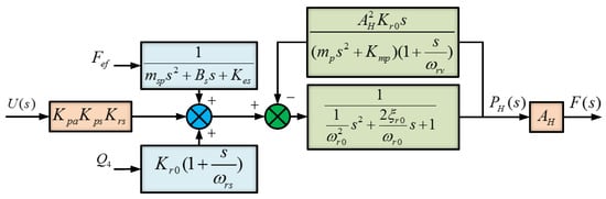
Figure 9.
Block diagram of the transfer function of the column hydraulic cylinder pressure control system.
Therefore, when external disturbances are not considered, the open-loop transfer function expression of the system is:
Based on the calculation of relevant parameters in Table 2, it is known that ωr0 = 18.54 Hz, ωrv = 187.5 Hz, and ωrA = 0.244 Hz. Substituting these parameters into Equation (33) yields the system’s open-loop transfer function.
Table 2.
The parameter table of column hydraulic cylinder pressure control system.
4.2. Modeling of Initial Support-Force Control System for Support Hydraulic Cylinder
Based on the mathematical modeling of the hydraulic cylinder pressure-control system, initial support-force setting, and support strength prediction, the controller in the control system is now constructed to achieve real-time tracking after importing the reasonable initial support-force value as the desired value into the control system. The initial support-force control system for the self-advancing temporary support hydraulic cylinder based on pressure feedback is shown in Figure 10.
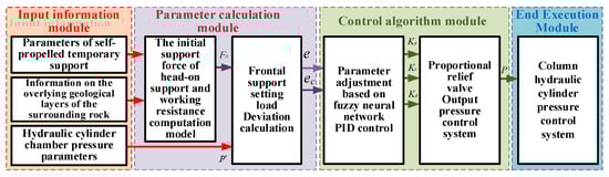
Figure 10.
System diagram of setting force control system based on pressure feedback.
- (1)
- Input information module
In the input information module, the structural parameters of hydraulic support equipment, geological layer information overlying the surrounding rock, and the real-time pressure measured by sensors in the hydraulic cylinder of the prop provide the parameter basis for calculating the initial support force;
- (2)
- Parameter calculation module
In the parameter calculation module, the established formulas for calculating the initial support force and working resistance of heading support are used to reasonably set the initial support force; the deviation and deviation rate of the heading support initial support force are calculated to provide input parameters for the control algorithm module;
- (3)
- Control algorithm module
In the control algorithm module, online tuning of PID control parameters is performed using a fuzzy neural network algorithm to control the output pressure of the proportional relief valve in the hydraulic support, thereby achieving adaptive adjustment of the heading support initial support force;
- (4)
- End execution module
Within the final control stage, electrical inputs actuate the proportional relief valve to modulate flow. This facilitates dynamic pressure regulation within the hydraulic actuator’s lower compartment, ensuring operational compliance with tunnel advancement support specifications.
4.3. Initial Support-Force Controller Design
The adoption of the FNN-PID controller is motivated by the critical need to address the inherent challenges of the hydraulic support-force control system. Conventional PID control suffers from fixed parameters, struggling with the system’s strong nonlinearity (e.g., flow-pressure characteristics of valves) and time-varying disturbances (e.g., roof load fluctuations and hydraulic parameter drift). While fuzzy PID offers improved adaptability to nonlinearities, its performance heavily relies on the quality of the predefined rule base and membership functions, which are difficult to optimize perfectly for complex, dynamic environments like the mining face and which may lack sufficient adaptability to unmodeled disturbances or long-term parameter changes.
The FNN-PID controller integrates the complementary strengths of fuzzy logic and neural networks to overcome these limitations. The fuzzy-logic component provides a structured framework to handle system nonlinearity and imprecise reasoning using linguistic rules, mimicking human-operator intuition. Crucially, the embedded neural network (a BP structure in this implementation) enables online, real-time learning and self-adaptation. This neural component continuously adjusts the PID parameters (Kp, Ki, Kd) based on the current error and its rate of change, effectively optimizing the controller’s response dynamically in the face of uncertainties and disturbances. This fusion allows the controller to automatically fine-tune itself to achieve both high tracking precision (minimizing steady-state error) and rapid response (reducing settling time and overshoot) under varying operating conditions, a capability difficult to achieve with either fuzzy PID or pure neural network PID alone [19,20,21]. The block diagram of the fuzzy neural network PID controller’s construction principle is shown in Figure 11.
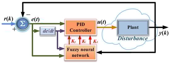
Figure 11.
Block diagram of crawler walking mechanism controlled by fuzzy neural network PID.
4.3.1. Fuzzy PID Controller
- (1)
- PID Controller
Considering the system’s nonlinearity, a fuzzy control algorithm is employed to achieve the optimal proportional, integral, and derivative PID control parameter ratios The difference e(t) between the desired displacement ri(k) and the actual displacement yi(k), along with its rate of change ec(t), serves as the input variables for the fuzzy PID controller. The relationship between these inputs and the output u(t) satisfies
where KP is the proportional gain; KI is the integral gain; and KD is the derivative gain.
A two-dimensional fuzzy controller is employed, with inputs identified as e(t) and its rate of change ec(t) and outputs as three correction parameters ΔKP, ΔKI, and ΔKD. The adjustment rules are as follows:
where K′P, K′I, and K′D are the preset initial values of the control parameters.
Based on the transfer function of the hydraulic pressure control system determined above, the Ziegler–Nichols tuning method is used to set the initial PID control parameters to 1.52, 0.12, and 0.15, respectively.
- (2)
- Fuzzy Logic Design
Drawing upon established control theory and expert knowledge, the deviation e(t) and its derivative ec(t) are assigned normalized domains: [−3, 3] for e(t), [−1.5, 1.5] for ec(t), and [−0.3, 0.3] for output variables. These continuous spaces are partitioned into seven linguistic classes: NB (Negative Big), NM (Negative Medium), NS (Negative Small), ZO (Zero), PS (Positive Small), PM (Positive Medium), and PB (Positive Big). Implementation employs the Mamdani inference scheme with two inputs and three outputs. Membership characterization utilizes triangular (trimf) and Z-shaped functions, while governing heuristics are codified in Table 3. Visual representations of input/output membership distributions appear in Figure 12 [22]. The Ziegler–Nichols tuning method is used to set the initial PID control parameters to 17.6, 0.7, and 0.2, respectively.
Table 3.
Rule base for fuzzy logical control.
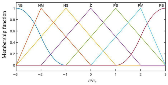
Figure 12.
The subordinating degree function of input and output.
4.3.2. Fuzzy Neural Network PID (FNN-PID) Controller
Illustrated in Figure 13, the fuzzy-neural architecture processes hydraulic cylinder pressure deviations and their temporal derivatives as dual inputs, generating three PID control parameters as outputs. This five-tiered network comprises sequential processing stages:
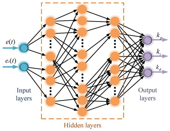
Figure 13.
Schematic diagram of fuzzy neural network structure.
- (1)
- Layer 1 (Fuzzification): 7 neurons mapping input signals to linguistic variables;
- (2)
- Layer 2 (Rule Inference): 49 neurons implementing fuzzy control heuristics;
- (3)
- Layer 3 (Defuzzification): 7 neurons converting fuzzy outputs to crisp values;
- (4)
- Input/output layers completing signal transduction pathways [23].
Based on the input and output structure of the fuzzy neural network shown in Figure 13, the following analysis is conducted:
- (1)
- The input layer of the fuzzy neural network has two signals: e(k) and ec(k), where k ∈ [0, t]. Their corresponding outputs are O1(1,j) = e(k) and O1(2,j) = ec(k), where j = 1, 2, …, 7;
- (2)
- During signal propagation from the input to fuzzification layer, the input–output transformation is mathematically represented as
- (3)
- Signal flow characteristics between the rule execution tier and defuzzification stage are defined as follows:
- (4)
- The inputs and outputs of the output layer are, respectively,
The error feedback-performance metric is established as: E(k) = 0.5[r(k) − y(k)]2,where r(k) denotes the desired reference value at discrete-time index k, and y(k) represents the measured system output. As y(k) converges to r(k), this quadratic cost functional asymptotically approaches its minimum value of zero. The neural network can be used to perform real-time calibration of the center value bij, width cij of the fuzzy membership function, and the weight coefficient λmn. The corresponding adjustment rules are
where ξ(k) is the learning rate of the neural network.
To dynamically synchronize the neural network’s learning rate with the deployed control architecture, we implement phased adaptive learning rate regulation. This staged approach maintains optimal algorithm training rigor and closed-loop control efficacy throughout autonomous learning cycles, governed by the following segmented rules:
The gradient components of the performance metric E(k) defined in Equation (40) are computed via the backpropagation algorithm. The relevant calculation methods are
In Equation (42), the calculation can be approximated by its variable sign function, thus yielding ; let .
5. Simulation Test of Initial Support-Force Control
Under the ideal model scenario, certain uncertain factors present in the actual operation of the hydraulic system are ignored. Based on the aforementioned controller design, experiments are conducted in a co-simulation environment of AMESim 2304 and Matlab/Simulink 2016. First, modules are constructed according to the mathematical modeling of the hydraulic cylinder pressure control system, and relevant parameters are selected to configure functional components. Matlab is utilized to generate simulation graphs, completing the analysis of simulation experimental results for the adaptive control of initial support force in self-shifting temporary supports [24].
5.1. Simulation Model Establishment
To assess the performance superiority of the adaptive control algorithm for primary support forces, computational implementation of standardized analytical expressions determines the target initial supporting-force magnitude based on fundamental resistance parameters. A step signal is employed to simulate input for tracking control of the initial support force. Based on the established mathematical model, elastic and damping loads are used to replace the roadway roof load model. Referring to the measured parameters of the No. 3 coal seam roof in a certain mine, the stiffness coefficient is set to 10,000 N/mm, and the damping coefficient is set to 10 N·s/m.
In AMESim, a model of the pressure regulation system for the hydraulic cylinder chamber of the self-shifting temporary support is established, as shown in Figure 14. Then, different controllers are constructed in Matlab/Simulink for simulation comparison. The Interface Block module is used to enable data exchange between AMESim and Matlab/Simulink, completing the dynamic simulation of the system, as shown in Figure 15. The fuzzy neural network algorithm is programmed based on the Matlab/Simulink compilation window, with a simulation time set to 10s. The Dormand–Prince numerical integration method (ode45) was employed for dynamic simulation, utilizing the hydraulic component specifications documented in Table 2.
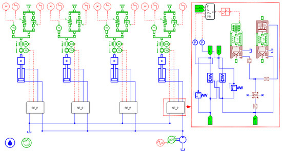
Figure 14.
The simulation model of hydraulic cylinder pressure control system based on AMESim.

Figure 15.
Joint simulation model based on AMEsim and Simulink.
5.2. Simulation Results Analysis
To validate fundamental control algorithm efficacy, the target support-force magnitude is determined through analytical expressions governing excavation support mechanics. This computed benchmark value serves as the reference input signal for the controller. In the simulation process, the test is divided into two situations: Situation A, the use of step signals and square wave signals to simulate the use of hydraulic cylinders with sudden loads and Situation B, the use of sinusoidal signals and sawtooth wave signals to simulate the use of hydraulic cylinders with continuous action.
Figure 16a shows that the FNN PID algorithm has a rise time of approximately 0.8 s under step signals, with overshoot controlled within 5%, a settling time (±2% error band) of about 1.5 s, and a steady-state error approaching zero. The Fuzzy PID has a rise time of about 1.2 s, an overshoot of around 8%, and a settling time of approximately 2.0 s. Using step signals to simulate sudden load conditions, the fast response and low overshoot characteristics of the FNN PID algorithm can effectively reduce impact vibrations in the hydraulic system, avoid seal wear caused by violent piston rod movements, and better suit the pressure control system of the self-shifting temporary support hydraulic cylinder.
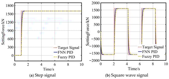
Figure 16.
Signal input response and error curves in Situation A.
Figure 16b indicates that the FNN PID algorithm has a peak tracking error of ±300 kN for square wave signals, a transition time of about 3.5 s, and low waveform distortion. The fuzzy PID algorithm has a peak tracking error of ±500 kN and a transition time of approximately 4.8 s. Using square wave signals to simulate frequent directional changes in the hydraulic cylinder, the low-error tracking capability of the FNN PID algorithm ensures consistent execution of end actions, reduces pressure fluctuations during directional changes, and minimizes impact losses in hydraulic valve groups, further enhancing system lifespan.
Figure 17a shows that the FNN PID algorithm maintains an amplitude error of ±150 kN in sine wave tracking, with a phase lag of approximately 5° and a frequency response bandwidth of 1.2 Hz. The fuzzy PID algorithm has an amplitude error of ±250 kN, a phase lag of about 10°, and a bandwidth of around 0.8 Hz. The wide frequency response and low phase lag characteristics of the FNN PID algorithm ensure precise trajectory control in high-frequency reciprocating motions of the hydraulic column system, preventing action delays caused by phase differences and improving the dynamic performance of servo control.
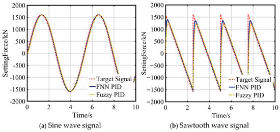
Figure 17.
Signal input response and error curves in Situation B.
Figure 17b indicates that the FNN PID algorithm exhibits a linear error slope of 0.08 kN/s in sawtooth wave tracking, with a steady-state error-fluctuation range of ±100 kN. The fuzzy PID has a linear error slope of 0.15 kN/s and a steady-state error fluctuation of ±180 kN. Using sawtooth wave signals to simulate continuous variable load conditions, the low linear error of the FNN PID algorithm ensures speed stability during uniform piston-rod movement, reduces speed fluctuations caused by gradual load changes, and is well-suited for hydraulic column systems requiring high displacement accuracy to effectively support coal-mine roof structures.
Based on the simulation results in Figure 18 and Figure 19 and Table 4, the FNN-PID algorithm demonstrates superior dynamic performance over fuzzy PID control. For step signals (Condition A), FNN-PID achieves a 51.3% faster rise time (0.55 s vs. 1.13 s), 52.3% lower overshoot (5.02% vs. 10.52%), and 39.4% reduced steady-state error (12.12 kN vs. 20.01 kN). During square-wave tracking, its maximum error is 49% smaller (±51.04 kN vs. ±100.11 kN) with 30% shorter transition time. These attributes effectively mitigate hydraulic impact vibrations and valve-group wear during abrupt load changes.
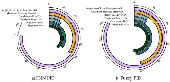
Figure 18.
Dynamic performance indicators of different control algorithms in Situation A.
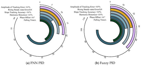
Figure 19.
Dynamic performance indicators of different control algorithms in Situation B.
Table 4.
Comparison of controller simulation results.
Under sinusoidal signals (Condition B), FNN-PID exhibits 40% smaller amplitude error (±150 kN vs. ±250 kN), 50% reduced phase lag (5° vs. 10°), and a 50% wider bandwidth (1.2 Hz vs. 0.8 Hz), ensuring precise trajectory control during high-frequency reciprocation. For sawtooth waves, its linear error slope is 46.7% lower (0.08 kN/s vs. 0.15 kN/s) with 44.4% narrower steady-state fluctuation (±100 kN vs. ±180 kN), maintaining piston-rod velocity stability under gradual loads. The integrated fuzzy-neural adaptation enables FNN-PID to suppress oscillations observed in fuzzy PID (Figure 18b and Figure 19b), achieving ±3.5% force-tracking accuracy critical for preventing roof delamination or compressive failure.
6. Engineering Validation Experiments
6.1. Hydraulic Support Test System
To verify the engineering applicability of simulation results and test the control algorithm’s performance in regulating initial support force under different loads, support tests were conducted on-site indoors. The experimental site is shown in Figure 20. The hydraulic support test system consists of five sets of hydraulic supports, powered by a hydraulic pump station. High-pressure hydraulic oil output from the pump station is delivered via pipelines to the hydraulic cylinders of each support, driving them to perform lifting and advancing actions. PPM-T230B pressure sensors are installed in the return oil circuit of each support’s hydraulic cylinder to collect real-time pressure data. These pressure data are transmitted as electrical signals to the controller panel. Operators can set the target pressure value on the controller panel according to test requirements. By adjusting components such as solenoid directional valves and proportional pressure-reducing valves in the hydraulic system, the pressure inside the hydraulic cylinder of the support column is dynamically regulated in real time, ensuring the hydraulic support maintains the set pressure condition throughout the test.
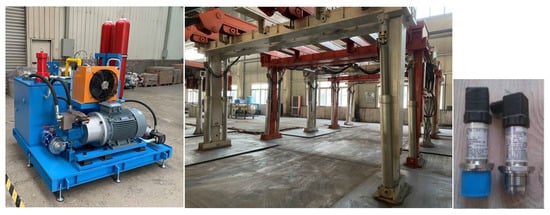
Figure 20.
The experimental site diagram of advanced support equipment.
6.2. Test Result Analysis
To minimize the impact of hydraulic equipment on the control algorithm, output pressure tests were first conducted on the five sets of hydraulic supports. Three target initial support-force levels were set: 1600 kN, 1300 kN, and 1100 kN, with each test repeated three times and the average taken. The hydraulic support with the smallest output error was selected for comparative tests of the control algorithm after each initial support-force test. The test results for different target initial support-force levels are shown in Figure 21, Figure 22 and Figure 23, and the regulation test data are recorded in Table 5.
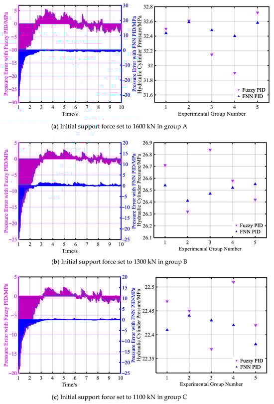
Figure 21.
Hydraulic cylinder pressure test results under different initial support-force settings.
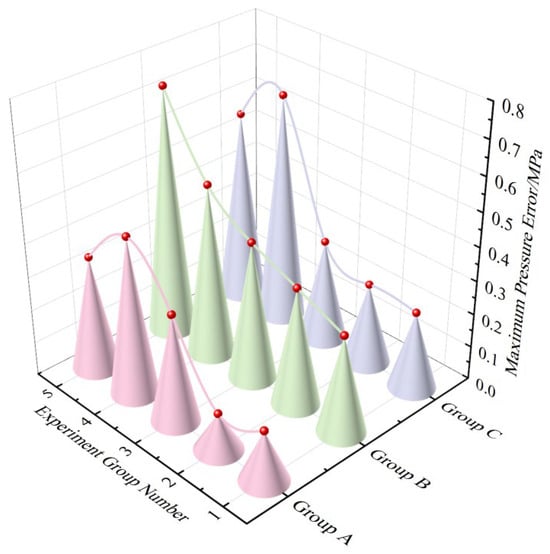
Figure 22.
Maximum pressure errors of each experimental group under different initial support forces in FNN PID control algorithm.
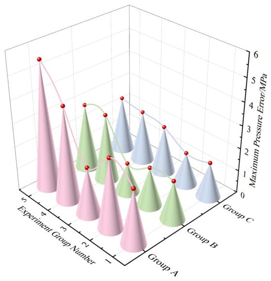
Figure 23.
Maximum pressure errors of each experimental group under different initial support forces in Fuzzy PID control algorithm.
Table 5.
The experimental data of adjustment and control of setting force of hydraulic support.
The measured data results indicate that the FNN PID outperforms the Fuzzy PID control algorithm in terms of pressure tracking accuracy and stability. When hydraulic supports bear roof pressure underground, the FNN PID leverages the self-learning capability of neural networks and the nonlinear adaptability of Fuzzy control to swiftly adjust control parameters and reduce pressure fluctuations when load changes abruptly or prolonged operation causes hydraulic oil-temperature variations. This ensures the pressure inside the hydraulic cylinder remains closer to the ideal state. In contrast, the Fuzzy PID, lacking the dynamic optimization ability of neural networks, exhibits response delays or oscillations under complex working conditions, thereby compromising the reliability and safety of hydraulic cylinder support.
Additionally, during actual hydraulic cylinder operation, nonlinear factors such as changes in hydraulic oil viscosity, pipeline leakage, and mechanical friction can cause the overshoot, settling time, and steady-state error of pressure response to exceed simulation test results. For instance, while the FNN PID’s response time to sudden load changes in simulations may be 0.5 s, real-world measurements—due to system inertia and damping—could extend this to 0.8 s, with pressure fluctuation amplitudes increasing by 10%~15%. Such discrepancies may degrade the actual motion precision of hydraulic cylinders, potentially leading to insufficient initial support force or overload during roof support, thereby affecting equipment lifespan and underground operational safety. Furthermore, while the adaptive capability of FNN PID in measured data still outperforms fuzzy PID, the attenuation of control effectiveness may lead to pressure instability in hydraulic cylinders during prolonged operation. This necessitates on-site parameter fine-tuning or hardware optimization to compensate for discrepancies between simulation and actual measurements.
7. Conclusions
- (1)
- The fracture characteristics of the roadway roof in fully mechanized excavation were analyzed, a thin-plate static model for the heading roof was established, and theoretical calculations for the initial support force and working resistance of heading support were completed, providing target reference inputs for subsequent control systems;
- (2)
- The pressure system model for the hydraulic cylinder of self-shifting temporary support columns was constructed, enabling real-time online adjustment of PID parameters via fuzzy neural network control algorithms. A co-simulation model integrating AMESim and Matlab/Simulink was developed, completing the modeling of the initial support-force regulation system for self-shifting temporary supports based on pressure feedback;
- (3)
- Co-simulation results and measured data demonstrate that the fuzzy neural network PID control proposed in this study exhibits superior dynamic response and target-tracking performance compared to fuzzy PID control algorithms.
Author Contributions
Conceptualization, R.L. and D.W.; methodology, D.W.; software, W.Z.; validation, D.W. and M.W.; formal analysis, R.L. and T.L.; resources, M.W.; funding acquisition, M.W. All authors have read and agreed to the published version of the manuscript.
Funding
This research was supported by Found of the National Natural Science Foundation of China grant number 52474187.
Data Availability Statement
The original contributions presented in this study are included in the article material. Further inquiries can be directed to the corresponding author.
Conflicts of Interest
The authors declare no conflict of interest.
References
- International Energy Agency. Global Coal Consumption Trends; International Energy Agency: Paris, France, 2023. [Google Scholar]
- Yuan, L.; Wang, E.; Ma, Y.; Liu, Y.; Li, X. Research progress of coal and rock dynamic disasters and scientific and technological problems in China. J. China Coal Soc. 2023, 48, 1825–1845. [Google Scholar]
- Hongpu, K.; Pengfei, J.; Fuqiang, G.; Ziyue, W.; Chang, L.; Jianwei, Y. Analysis on stability of rock surrounding heading faces and technical approaches for rapid heading. J. China Coal Soc. 2021, 46, 2023–2045. [Google Scholar]
- Jia-Sheng, C.; Ming-zhong, G. Research on integration of roadway excavation, bolting, support, and detection. Procedia Eng. 2011, 26, 869–875. [Google Scholar] [CrossRef][Green Version]
- Ding, W.; Zhao, S.; Chen, Y. A novel type of overrun support for general mining roadways. Int. J. Min. Sci. Technol. 2020, 30, 687–695. [Google Scholar][Green Version]
- Evans, W. Design of support systems for mine roadways. Min. Eng. 1981, 33, 521–528. [Google Scholar][Green Version]
- Wang, G.; Hu, X.; Liu, X.; Yu, X. Adaptability analysis of four-leg hydraulic support for underhand working face with large mining height of kilometer deep mine. J. Min. Sci. 2020, 45, 865–875. [Google Scholar][Green Version]
- Cheng, J.; Wan, Z.; Peng, S.; Zhang, H.; Xing, K.; Yan, W.; Liu, S. Technology of intelligent sensing of longwall shield supports statusand roof strata based on massive shield pressure monitoring data. J. Min. Sci. 2020, 45, 2090–2103. [Google Scholar][Green Version]
- Zhao, H.; Ma, H.; Wu, M. Dynamic response of advanced support equipment in roadway excavation. J. Vib. Control 2022, 28, 1234–1245. [Google Scholar][Green Version]
- Peng, S. Coal Mine Ground Control; Society for Mining, Metallurgy & Exploration: Englewood, CO, USA, 2008. [Google Scholar]
- Hu, X.; Liu, X.; Pang, Y.; Liu, W. Adaptive control of setting load of hydraulic support based on BP neural network PID. J. Min. Sci. Technol. 2020, 5, 662–671. [Google Scholar][Green Version]
- Xue, G.; Guan, J.; Chai, J.; Zhang, H.; Qu, Y.; Wu, M. Adaptive control of advance bracket support force in fully mechanized roadway based on neural network PID. J. China Coal Soc. 2019, 11, 3597–3603. [Google Scholar][Green Version]
- Xu, Z.; Li, C.; Cao, Y.; Tai, L.; Han, J. A case study on new high-strength temporary support technology of extremely soft coal seam roadway. Sci. Rep. 2023, 13, 21333. [Google Scholar] [CrossRef] [PubMed]
- Yang, T.; Sun, N.; Fang, Y. Adaptive fuzzy control for uncertain mechatronic systems with state estimation and input nonlinearities. IEEE Trans. Ind. Inform. 2021, 18, 1770–1780. [Google Scholar] [CrossRef]
- Yang, X.; Deng, W.; Yao, J. Neural adaptive dynamic surface asymptotic tracking control of hydraulic manipulators with guaranteed transient performance. IEEE Trans. Neural Netw. Learn. Syst. 2022, 34, 7339–7349. [Google Scholar] [CrossRef] [PubMed]
- Li, G.; Ma, F.S.; Guo, J.; Zhao, H.J. Experimental research on deformation failure process of roadway tunnel in fractured rock mass induced by mining excavation. Environ. Earth Sci. 2022, 81, 243. [Google Scholar] [CrossRef] [PubMed]
- Hong, Z.; Tao, M.; Wu, C.; Zhou, J.; Wang, D. The spatial distribution of excavation damaged zone around underground roadways during blasting excavation. Bull. Eng. Geol. Environ. 2023, 82, 155. [Google Scholar] [CrossRef]
- Wang, Q.; Zhang, C.; Qiu, S. The study on electro-hydraulic proportional relief valve of disc braking system based on AMESim. In Proceedings of the 2015 International Conference on Intelligent Systems Research and Mechatronics Engineering, Zhengzhou, China, 11–13 April 2015; Atlantis Press: Dordrecht, The Netherlands, 2015; pp. 980–983. [Google Scholar]
- Chen, J.S.; Yang, Z.H. On the asymmetric line-contact deformation between two planar elasticae. Int. J. Solids Struct. 2022, 256, 111991. [Google Scholar] [CrossRef]
- Zhong, Q.; Xu, E.G.; Jia, T.W.; Yang, H.Y.; Zhang, B.; Li, Y.B. Dynamic performance and control accuracy of a novel proportional valve with a switching technology-controlled pilot stage. J. Zhejiang Univ. Sci. A 2022, 23, 272–285. [Google Scholar] [CrossRef]
- Wang, G.; Qiao, J. An efficient self-organizing deep fuzzy neural network for nonlinear system modeling. IEEE Trans. Fuzzy Syst. 2021, 30, 2170–2182. [Google Scholar] [CrossRef]
- Shi, J. An interval type-3 fuzzy PID control system design and its application in solid oxide fuel cells power plant. J. Intell. Fuzzy Syst. 2023, 45, 11149–11162. [Google Scholar] [CrossRef]
- Zhao, J.; Chang, D.; Cao, B.; Liu, X.; Lyu, Z. Multiobjective evolution of the deep fuzzy rough neural network. IEEE Trans. Fuzzy Syst. 2024, 33, 242–254. [Google Scholar] [CrossRef]
- Buhaianu, A.R.; Dinca, L.; Dumitrache, A.; Benec-Mincu, G.M. Numerical simulations of some characteristics for electrohydrostatic actuators used in aviation. In AIP Conference Proceedings, Proceedings of the International Conference of Numerical Analysis and Applied Mathematics: ICNAAM2022, Heraklion, Greece, 19–25 September 2022; AIP Publishing: Melville, NY, USA, 2024; Volume 3094. [Google Scholar]
Disclaimer/Publisher’s Note: The statements, opinions and data contained in all publications are solely those of the individual author(s) and contributor(s) and not of MDPI and/or the editor(s). MDPI and/or the editor(s) disclaim responsibility for any injury to people or property resulting from any ideas, methods, instructions or products referred to in the content. |
© 2025 by the authors. Licensee MDPI, Basel, Switzerland. This article is an open access article distributed under the terms and conditions of the Creative Commons Attribution (CC BY) license (https://creativecommons.org/licenses/by/4.0/).