Article

Optimizing a Sustainable Inventory Model Under Limited Recovery Rates and Demand Sensitivity to Price, Carbon Emissions, and Stock Conditions

1
Department of Distribution Management, Takming University of Science and Technology, Taipei 114, Taiwan
2
Institute of Industrial Management, National Central University, 300 Zhongda Road, Zhongli District, Taoyuan City 32001, Taiwan
*
Author to whom correspondence should be addressed.
Mathematics 2025, 13(18), 2916; https://doi.org/10.3390/math13182916
Submission received: 25 July 2025 / Revised: 2 September 2025 / Accepted: 5 September 2025 / Published: 9 September 2025

Abstract

The recovery, rework, or remanufacturing of returned products has received significant attention, leading to considerable advancements in green supply chain management. However, the impact of recovery mechanisms under demand sensitivity remains understudied. This study develops a sustainability model that incorporates limited recovery rates and demand sensitivity to price, carbon emissions, and stock conditions. The analysis investigates the difference in profit when considering recovery and proposes a procedure for deriving optimal solutions using two key decision variables: unit sales price and cycle time, within a nonlinear profit model. The findings show that (i) the increase in total profit is significant and (ii) both sellers and consumers benefit from this mechanism. In addition, total profit is 15% higher, while the total cost is 22% lower than in the case without recovery. Consumers can purchase products at lower prices (−12%), and sellers can sell more products (+4%), thereby earning higher profit (+15%). Such a win–win policy aligns with environmental, social, and governance (ESG) regulations and supports a healthy, long-term supply chain relationship. Numerical examples and sensitivity analysis illustrate the characteristics of the proposed model. The results also provide managerial insights into enterprises’ limited recovery capacity.

1. Introduction

Within the paradigm of sustainable supply chain management, the reuse and overhaul of returned products—through recovery, rework, or remanufacturing—has been prioritized like never before, reflecting their growing importance in achieving both environmental and economic goals.
Dwicahyani et al. [1] proposed a closed-loop supply chain model involving a retailer, manufacturer, and supplier, where the return rate functionally depends on the acceptance quality level of returned items. The manufacturer operates an imperfect regular production process that yields some defective units, which are inspected and either reworked, remanufactured using recoverable returns, or, if not fully recoverable, refurbished and sold in a secondary market at a discount.
Mahato and Mahata [2] developed a profit-maximizing green EOQ model under capacity constraints by integrating order-size-dependent trade credit, all-unit discounts, partial backorder, and carbon emissions minimization. They demonstrated that retailers with limited in-house warehouse space can enhance both profitability and environmental performance by placing larger orders and renting additional storage capacity.
Inventory models that address recovery issues and environmental, social, and governance (ESG) considerations have received significant attention, as defining stock dynamics that align with ESG requirements is highly effective [3]. However, the difference between considering and not considering recovery has not yet been thoroughly investigated and quantified. Since contemporary markets are highly competitive, cost-sensitive, and environmentally conscious, such issues remain challenging when market demand is sensitive to selling prices, stock inventory levels, and carbon emissions [4]. Yu et al. [5] considered an inventory model that integrated manufacturer–retailer operations in a closed-loop setup, where both customer demand and return behavior shift in response to price changes. Hasan et al. [6] developed an eco-friendly inventory model that demonstrates how emissions are influenced by three types of carbon policies: taxes, offset schemes, and cap-and-trade systems.
Mabini et al. [7] considered a multi-product model in the case of shortage. Wee [8] optimized a joint pricing and replenishment model with price-dependent demand. Giri and Chaudhuri [9] and Teng and Chang [10] derived economic production quantity (EPQ) models with stock-dependent demand. Shaikh et al. [11] addressed an inventory model with price- and stock-dependent demand. Other studies focused on recovery, rework, or remanufacturing. For instance, Schrady [12] was the earliest to propose an EOQ model with recovery under deterministic demand. Subsequent researchers extended Schrady’s analysis: Nahmias and Revera [13] investigated finite remanufacturing rates, and Koh et al. [14] examined finite manufacturing and remanufacturing rates.
Until recently, the sustainability concept of ESG had attracted more attention for reasons beyond classical cost considerations. Maity et al. [15] developed an eco-friendly EOQ model that accounts for carbon emissions using a pentagonal intuitionistic dense fuzzy framework. Khan et al. [16] presented a model that integrates prepayment installments, pricing, and restocking decisions for product growth, considering demand that follows a power curve, nonlinear storage costs, and carbon regulation rules.
Hua et al. [17] developed an EOQ model using the cap-and-trade mechanism to reduce carbon emissions. Inderfurth et al. [18] derived lot-sizing decisions in a hybrid production/rework system considering defective products. Chung et al. [19] developed a closed-loop inventory system for a vendor and a buyer considering a single manufacturing/remanufacturing cycle with constant demand. Yang et al. [20] extended Chung et al.’s model to evaluate multiple manufacturing/remanufacturing cycles. Hovelaque and Bironneau [21] investigated a sustainable EOQ model with carbon-emission-dependent demand. Helmrich et al. [22] formulated an economic lot-sizing problem with emission capacity constraints. Ghosh et al. [23] optimized a lot-sizing problem with a strict carbon cap policy and stochastic demand. Aljuneidi and Bulgak [24] addressed a facility-location problem considering the carbon footprint of reverse logistics with constant demand. Chan et al. [25] established a vendor–retailer–recycler inventory system by using a genetic algorithm. Konstantaras et al. [26] optimized a closed-loop inventory system with time-varying demand and carbon tax regulations. Sarkar and Guchhait [27] examined the impact of information asymmetry on green supply chains, incorporating cap-and-trade policies, service levels, and vendor-managed inventory strategies. They utilized RFID technology to mitigate asymmetry and improve coordination.
Carbon taxes determine prices, stabilizing the cost of emissions for firms and enabling predictable long-term planning. For instance, carbon taxes in Sweden and British Columbia have led to material reductions in emissions—transport emissions in Sweden fell by 11%, while British Columbia achieved a 5–15% decline. However, carbon taxes do not guarantee emission outcomes. If the rate is set too low, emissions reductions may fall short of targets, exposing weaknesses in the policy.
Conversely, cap-and-trade systems set a fixed emissions quantity and thus ensure compliance with environmental goals; however, they are prone to volatile price signals. This volatility discourages firms from making low-carbon investments due to the uncertainty of allowance costs. Hybrid designs address these trade-offs effectively. For example, incorporating a price floor and ceiling (“safety valve”) in cap-and-trade provides emission certainty while cushioning price volatility, thereby striking a balance between the virtues of both instruments. Empirical modeling suggests that hybrid systems yield superior outcomes compared to either approach alone. In China, pairing a carbon tax with its Emissions Trading System (ETS) is projected to reduce CO2 emissions by an additional 32 million tons by 2030 relative to relying solely on a cap-and-trade approach.
There are various instances where recovery technologies, such as eccentric disk pumps, have been introduced into hygienic manufacturing operations, resulting in significant improvements in the product recovery ratio and operational expenditures [28]. Recovery strategies also support the development of new industry sectors. For instance, increased material costs motivate the automotive, personal computer, and cellular phone industries to reuse materials and items [29]. Sarkar and Bhuniya [30] developed a model focusing on flexible manufacturing and remanufacturing with green investments under variable demand. Their work emphasizes the integration of service facilities to enhance customer satisfaction and sustainability. Lin et al. [31] analyzed when firms should remanufacture in-house vs. outsource under distinct sales/return lifecycles, explicitly addressing remanufacturing capacity/constraints that limit effective recovery. Sebatjane [32] reviewed 140 papers on sustainable inventory models under carbon emission regulations, including carbon taxes, cap-and-trade schemes, and cap-and-offset schemes. A taxonomy was developed to classify existing models, and the reviewed studies were categorized accordingly. Research gaps were identified to outline a future research agenda. Table 1 presents the differences between this and existing studies, offering a more detailed comparison with sustainable inventory models in the literature.
This study differs in that it integrates new and used products into a production line. Based on ISO-developed CE (Circular Economy) standards and the resource flow assessment of a full product lifecycle, the successful integration of new and used products into a single production line is second only to zero-resource utilization, extending product lifespan and promoting resource reuse. This model addresses the urgent need for raw materials and high energy efficiency in the manufacturing industry. Combining new and used products creates dual value within the company: not only are raw material consumption and waste emissions reduced, but new revenue-generating business models are created. Academia and industry have widely recognized that supply chain innovations centered on recycling, reuse, and remanufacturing can significantly reduce pressure on raw material extraction, mitigate the risk of resource depletion, and create new cost and environmental benefits (for example, in the application of recycled electric vehicle batteries, remanufacturing significantly reduces manufacturing costs and carbon footprint). This strategy leverages the potential of integrating the circular economy with international Industry 4.0 technologies, such as using smart manufacturing methods to promote closed resource loops and implementing reverse supply chain management, thereby improving manufacturing efficiency and supporting sustainable development.
Market demand is sensitive to selling price, stock inventory levels, and carbon emissions. A manufacturer with recovery is considered a system. There are two product sources: products can be purchased from an external vendor or produced within the recovery factory. Used products can be recycled and recovered as new products.
This study proposes a sustainable EOQ model, where the cycle time is assumed to be stably synchronized with that of the recovery process. This assumption is adopted because allowing production and recovery cycles to vary independently introduces realism at the expense of analytical simplicity. It can increase in-process inventory and cycle variability, reduce the cost efficiencies predicted by classic EOQ models, and require more complex, adaptive scheduling strategies. When cycles are not synchronized, the hidden inventory cost increases, potentially raising the total operational costs unless the model is reoptimized with revised data. Without synchronized cycles, discrepancies between production and recovery timings result in buffer accumulation, particularly at upstream bottlenecks. As the Theory of Constraints notes, this creates waste in flow and increases work-in-progress (WIP) inventory and lead time variability. A variable synchronization approach, by contrast, can reduce these inefficiencies [4]. The effects of unsynchronized cycles can be summarized as follows: increased WIP inventory and higher holding costs disrupt the cost-optimal cycle, the EOQ assumptions no longer hold, and more complex scheduling (such as multiple deliveries and buffers) is required.
A total profit system (including sales revenue, minus the purchase cost of new and used products, minus the scrap disposal cost, minus the carbon emission cost, minus the classical and recovery setup costs, and minus the holding costs) is optimized to derive two independent decision variables: selling price and cycle time. The corresponding solution procedure is proposed in this study. Numerical examples are used to illustrate the difference in total profit when considering and not considering recovery. Sensitivity analysis is also conducted to identify significant parameters and their impact on decision variables. This research aims to help companies explore feasible solutions that both meet ESG standards while also increasing profits. The objective is to maximize the total profit of the sustainable inventory model, which considers limited recovery rates and demand sensitivity to price, carbon emissions, and stock conditions.

2. Mathematical Modelling

The mathematical model in this study is developed based on the following assumptions:
  • The replenishment rate is instantaneous, and the lead time is constant.
  • Market demand is sensitive to selling price, carbon emissions, and stock level.
  • The used product is recovered as a new product.
  • Cycle times for EOQ models and for recovery are assumed to be synchronized in a steady state.
  • Cap-and-trade regulations are adopted.
Notations are defined as in the following Table 2:
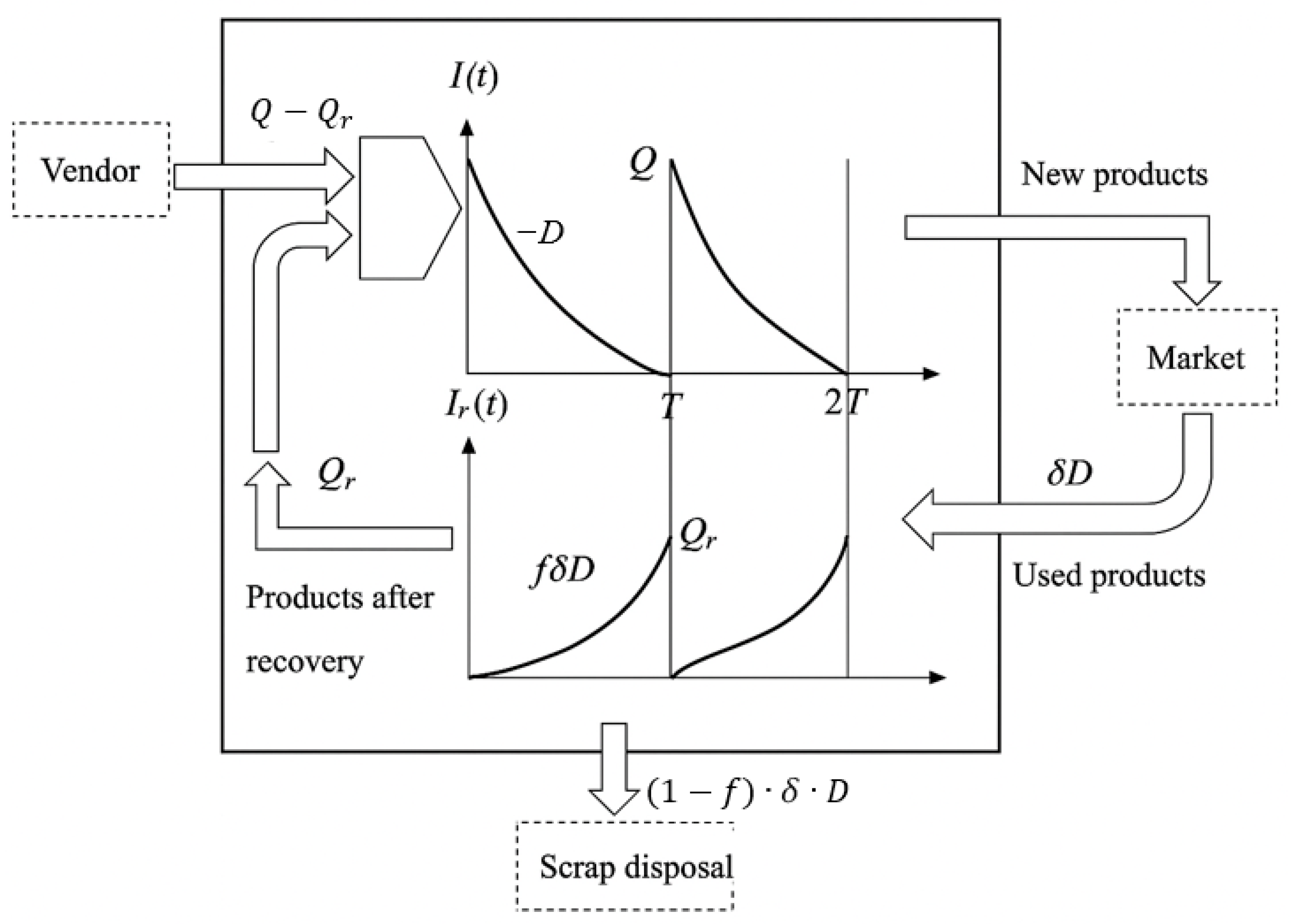
The flow of an EOQ model considering recovery in a mixed production system is illustrated in Figure 1. There are two sources of incoming products: outside vendors and the recovery factory. The old products can be recycled and recovered, and their recycling rate and recovery rate are δ and f, respectively.
Since the inventory level is depleted due to a demand that is sensitive to selling price, carbon emissions, and stock on hand, the inventory levels of the EOQ model and recovery factory are represented by the following differential equations, respectively:
d I t d t + γ I t = α β P κ E ,   0 t T
and
d I r t d t f δ γ I r t = + f δ α β P κ E ,   0 t T
The boundary conditions are I 0 = 0 and I r 0 = 0 .
The above equations were solved by Spiegel [35]:
I t = α β P κ E γ e γ T t 1 ,   0 t T
and
I r t = α β P κ E γ e f δ γ t 1 ,   0 t T
The lot size (denoted as Q) and the recovery lot size (denoted as Qr) can be expressed as I 0 and I r T , respectively, as shown below:
Q = α β P κ E γ [ e γ T 1 ] α β P κ E T ( 1 + 1 2 γ T )
and
Q r = α β P κ E γ e f δ γ T 1 α β P κ E f δ T 1 + 1 2 f δ γ T
The average demand can be obtained from the following:
A v e r a g e   d e m a n d = 1 T P Q = 1 T 0 T α β P k E + r I t d t α β P k E 1 + 1 2 r T
The proof is shown in Appendix A.
The annual sales revenue (denoted as SR) is formulated as
S R = 1 T P Q = α β P κ E ( 1 + 1 2 γ T )
The annual purchase cost (denoted as PC) is
P C = 1 T c Q Q r + u 3 δ Q = α β P κ E [ 1 + 1 2 γ T c + u 3 δ f δ 1 + 1 2 f δ r T c ]
The annual scrap disposal cost (denoted as SDC) is
S D C = 1 T 1 f δ Q = ( 1 f ) δ ( α β P κ E ) ( 1 + 1 2 γ T ) u 4
The annual carbon emission of the classical EOQ model (denoted as Ec) is
E c = S c T + H c T 0 T I t d t = S c T + H c T 2 α β P κ E  
The annual carbon emission of the recovery (denoted as Er) is
E r = S r c T + H r c T 0 T I r t d t = S r c T + H r c f δ T 2 α β P κ E
The total carbon emission (denoted as E) is defined in Equation (13), as the sum of E c and E r .
E = E c + E r
Solving the simultaneous equations of Equations (11)–(13), one can obtain Ec and Er, as shown in Equations (14) and (15), respectively:
E c = H r c f δ k T S c + 2 S c + H c T 2 α H c T 2 β P S r c H c k T T ( H r c f δ k T + H c k T + 2 )
and
E r = H r c f δ α T 2 H r c f δ β P T 2 H r c f δ T k S c + S r c H c T k + 2 S r c T ( H r c f δ T k + H c T k + 2 )
Referring to Hua et al. [17], the annual carbon emission cost (denoted as CEC) can be expressed as
C E C = E c + E r u 1 + E c + E r Z u 2
The annual classical cost (denoted as CC) excluding carbon-emission-related costs is
C C = S T + H 0 T I t d t = S T + H T 2 ( α β P κ E )
The annual recovery cost (denoted as RC) is
R C = S r T + H r T 0 T I r t d t = S r T + H r f δ T 2 α β P κ E
The annual total profit (denoted as TP) is
T P ( P , T ) = S R P C S D C C E C C C R C
The optimization problem of maximizing TP is a constrained nonlinear process, stated as
M a x i m i z e   T P ( P , T ) = S R P C S D C C E C C C R C
and is subject to Equations (12)–(14).
After substituting Equations (13)–(15) into Equations (8)–(10) and (16)–(18), there are two independent variables left, P and T, as shown in Equation (19).
Special Scenarios:
If the price-sensitive parameter β, carbon-emission-sensitive parameter κ, and stock-dependent parameter γ in Equation (19) are equal to zero, the demand is a constant, D = α, with independent variable (T) left. Then, one can solve the economic order cycle time by equating the first derivatives with respect to variable T to zero for the following five special scenarios:
  • For the EOQ model that neglects carbon emissions and recovery, where β, γ, κ, δ, Sc, Hc, Sr, Hr, Src, and Hrc are equal to zero, the economic order quantity and its cycle time are
T = 2 S α H   o r   Q = 2 S H
which is the same as the classical EOQ formula.
2.
For the EOQ model that considers carbon emissions but neglects recovery, where β, γ, κ, δ, Sr, Hr, Src, and Hrc are zero, the economic order cycle time is
T = 2 [ S + ( u 1 + u 2 ) S c ] α [ H + ( u 1 + u 2 ) H c ]   o r   Q = 2 α [ S + ( u 1 + u 2 ) S c ] [ H + ( u 1 + u 2 ) H c ]
3.
For the EOQ model that considers recovery but neglects carbon emissions, where β, γ, κ, Sc, Hc, Src, and Hrc are zero, the economic order cycle time is
T = 2 ( S + S r ) α ( H + δ f H r )   o r   Q = 2 α ( S + S r ) ( H + δ f H r )
4.
For the EOQ model that considers recovery and carbon emissions, where β, γ, and κ are zero, the economic order cycle time is
T = 2 [ S + S r + ( u 1 + u 2 ) ( S c + S r c ) ] α [ H + δ f H r + ( u 1 + u 2 ) ( H c + δ f H r c ) ]
or
Q = 2 α [ S + S r + ( u 1 + u 2 ) ( S c + S r c ) ] [ H + δ f H r + ( u 1 + u 2 ) ( H c + δ f H r c ) ]
5.
For the EOQ model that considers recovery, carbon emissions, and stock-dependent demand, where β and κ are zero, the economic order cycle time is
T = 2 [ S + S r + ( u 1 + u 2 ) ( S c + S r c ) ] α { H + δ f H r + u 1 + u 2 H c + δ f H r c + r [ c 1 δ 2 f 2 + δ u 4 1 f P δ u 3 ] }
In the five abovementioned scenarios, since T P ( P , T ) P = α > 0 , the total profit increases monotonically with the selling price (P).

3. Solution Procedure

If the price-sensitive parameter β, stock-dependent parameter γ, and carbon-emission-sensitive parameter κ are not zero, there are two independent variables in Equation (19), P and T. It is difficult to find closed-form analytical solutions for the nonlinear total profit function; fortunately, it can be derived numerically. To obtain the global optimal solution, the optimal solution of TP(P, T) in Equation (19) must satisfy the following four conditions. The proof of global optimality is shown in Appendix B.
The concave property of the TP function is examined. The following simple but efficient search algorithm is developed to find the optimal value of P and T .
Step 1: Input all parameters.
Step 2: Find the optimal unit sales price, P and cycle time T , by taking the first derivative of T P ( P ,   T ) with respect to P and T setting to zero simultaneously.
Step 3: To satisfy the conditions
2 T P ( P , T ) P 2 < 0   o r   2 T P ( P , T ) T 2 < 0
and
2 T P ( P , T ) P 2 2 T P ( P , T ) T 2 T P P , T P T P P , T T 2 > 0
Step 4. The optimal solution is obtained.
Note that the computing software Maple 18 was developed for this purpose and is implemented to derive the optimum solution for each problem.

4. Numerical Example

The preceding theory can be illustrated by a practical numerical example, where the source data were provided by a local company, Yiming Co., Ltd., New Taipei City, Taiwan, which belongs to A&1 Group. The factory produces consumer goods and utensils through plastic injection molding and metal extrusion molding and sells to large-scale hypermarkets.
Setup cost per cycle, S = USD 280;
Holding cost per unit per year, H = USD 135;
Carbon emissions per setup, Sc = 56 units;
Carbon emissions for each holding unit per year, Hc = 45 units;
Recovery setup cost per cycle, Sr = USD 65;
Recovery holding cost per unit per year, Hr = USD 40;
Recovery carbon emissions per setup, Src = 14 units;
Recovery carbon emissions for each holding unit per year, Hrc = 13 units;
Unit purchase cost, c = USD 330;
Unit purchase cost for used product from market, u 3 = USD 100;
Unit disposal cost for each recovery scrap, u 4 = USD 50;
Recycle rate of used product from market, δ = 0.8;
Yield rate from recovery, f = 0.85;
Unit carbon tax, u 1 = USD 2.5;
Carbon credit, Z = 300 units;
Unit carbon trading price, u 2 = USD 3;
Fixed demand parameter, α = 200;
Price-sensitive parameter, β = 0.18;
Carbon-emission-sensitive parameter, κ = 0.16;
Stock-sensitive parameter, γ = 0.25.
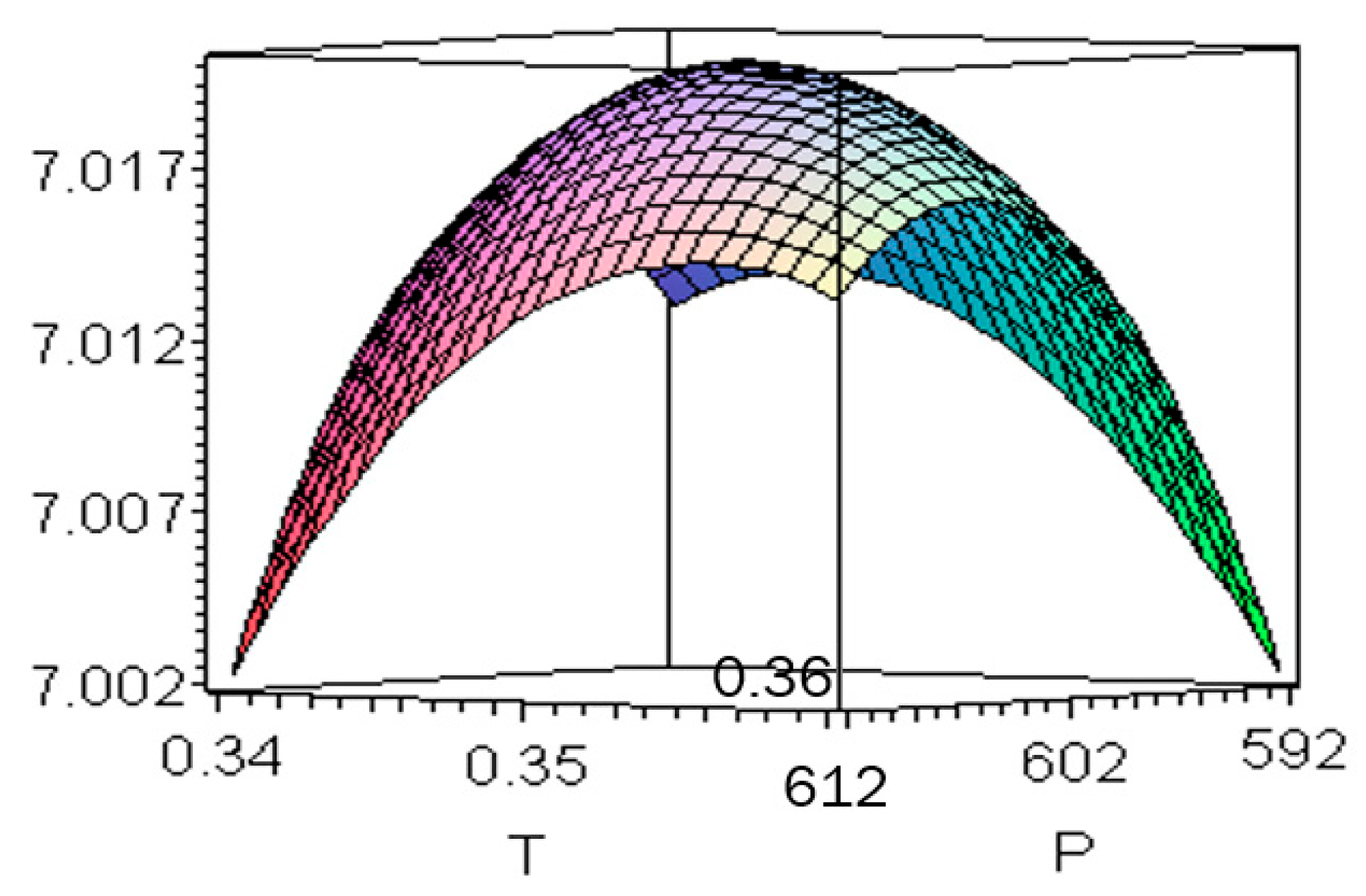
The graph of total profit with respect to P and T is shown in Figure 2.
When recovery is considered, not only is the total profit higher than 15%, but the total cost is also 22% lower than the case without considering recovery, mainly because the purchase cost is 40% lower. Other reasons are that the selling price is 12% lower and the demand is 4% higher. This is a win–win policy for both sellers and consumers. The consumer can buy products at lower prices (−12%), and the seller can sell more products (+4%) and earn more profit (+15%). Please see Table 3.

5. Sensitivity Analysis

To avoid repeating similar observations, the results of the sensitivity analysis of parameters affecting the profitability of the recovery policy are presented in two categories: the cost- and demand-based parameters.

5.1. The Demand-Based Parameters

The decision variables are influenced by a set of demand-based parameters, Φ1 = {α, β, κ, and γ}. These parameters are examined by changing them by ±5% and ±10%, resulting in the decisions shown in Table 4, Table 5, Table 6 and Table 7. The dependent variables {TP, TC, SR, Q , Q r , and PTPC} are also recorded. The relationships between known parameters and the decision variable are illustrated in Figure 3, Figure 4, Figure 5 and Figure 6.
From Table 4 and Figure 3, when the demand’s fixed parameter (α) increases, the selling price and the dependent variables {TP, TC, SR, Q , Q r , and PTPC} increase simultaneously.
Table 4. Sensitivity analysis of fixed parameter α.
αPTTPTCSR Q Q r PTPC (%)
220644.30.315210,073938219,4569.5176.39343.5
210623.20.33158472864817,1199.1066.11420.7
{200}602.50.35037020791414,9348.6825.8250.0
190582.30.37215717718112,8978.2425.525−18.6
180562.80.37804558644611,0047.7835.212−35.1
Note: Basic column; percentage of total profit change (PTPC) = T P T P / T P .
Figure 3. Unit sale price and lot size vs. α. Summary: With the fixed demand parameter, TP increases as α increases, directly and significantly impacting TP.
Mathematics 13 02916 g003
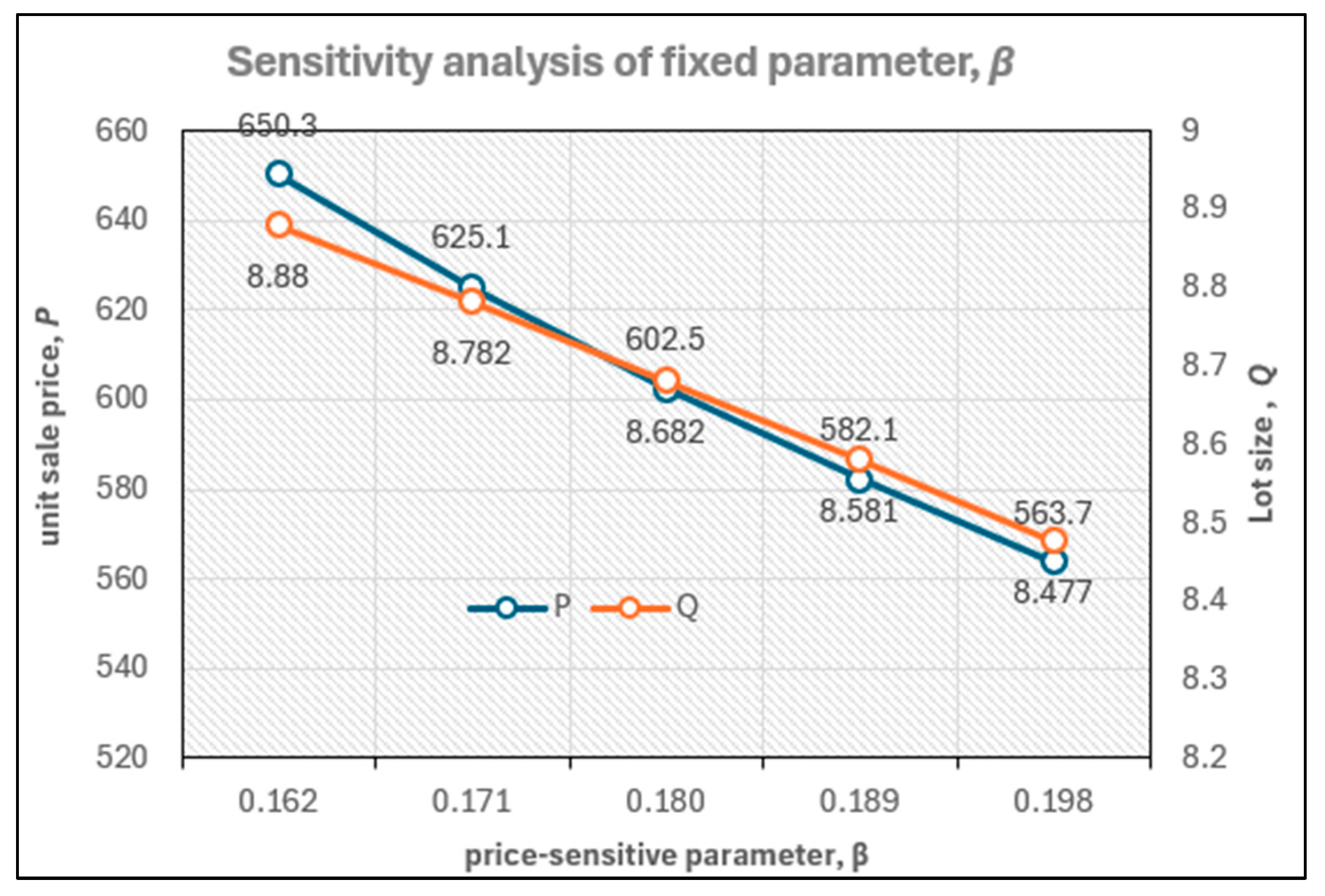
From Table 5 and Figure 4, the selling price (P) and lot size ( Q ) decrease when the price-sensitive parameter (β) increases. This suggests that lowering the price helps offset the effect of a higher price-sensitive parameter.
Table 5. Sensitivity analysis of price-sensitive parameter β.
βPTTPTCSR Q Q r PTPC (%)
0.198563.70.36135679754713,2268.4775.685−19.1
0.189582.10.35576313773214,0458.5815.755−10.1
{0.180}602.50.35037020791414,9348.6825.8250.0
0.171625.10.34517811809615,9078.7825.89311.3
0.162650.30.34028700827616,9758.8805.95923.9
Note: Basic column; percentage of total profit change (PTPC) = T P T P / T P .
Figure 4. Unit sale price and lot size vs. β. Summary: With the price-sensitive parameter, TP decreases as β increases, directly and significantly impacting TP.
Mathematics 13 02916 g004
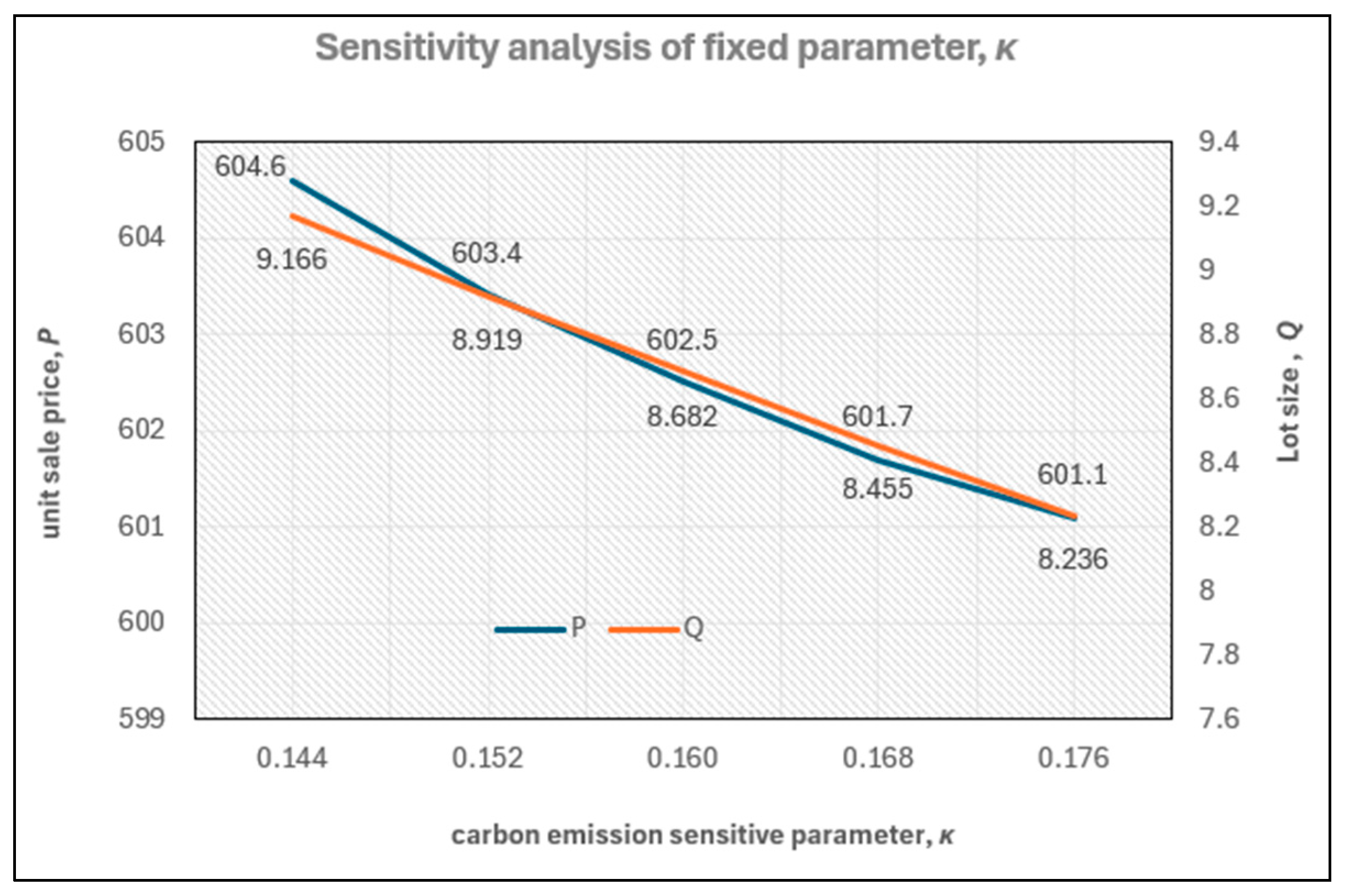
From Table 6 and Figure 5, higher carbon-emission-sensitive parameters result in a smaller lot size ( Q ), thereby reducing carbon emissions. The patterns shown in Figure 4 and Figure 5 are identical.
Table 6. Sensitivity analysis of carbon-emission-sensitive parameter κ.
κPTTPTCSR Q Q r PTPC (%)
0.176601.10.37056159720413,3648.2365.521−12.3
0.168601.70.36036572754914,1218.4555.670−6.4
{0.160}602.50.35037020791414,9348.6825.8250.0
0.152603.40.34057507830015,8078.9195.9866.9
0.144604.60.33108036870816,7459.1666.15414.5
Note: Basic column; percentage of total profit change (PTPC) = T P T P / T P .
Figure 5. Unit sale price and lot size vs. κ. Summary: With the carbon-emission-sensitive parameter, TP decreases as κ increases; however, the effect is weaker than that of β.
Mathematics 13 02916 g005
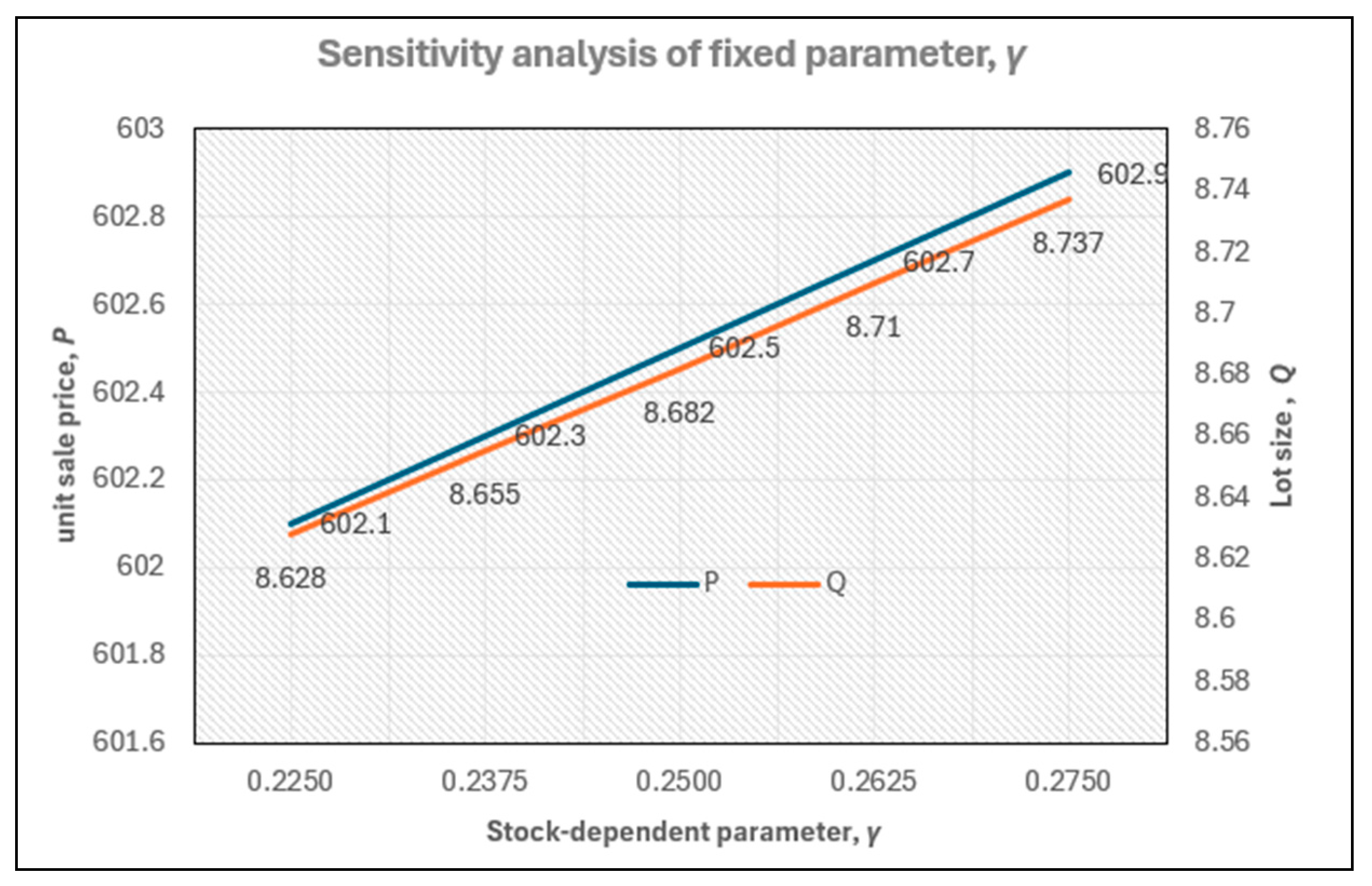
An increase in stock-dependent parameter (γ) leads to a larger lot size ( Q ) and higher sales revenue (see Table 7 and Figure 6).
Table 7. Sensitivity analysis of stock-sensitive parameter γ.
γPTTPTCSR Q Q r PTPC (%)
0.2750602.90.35147055793214,9888.7375.8530.5
0.2625602.70.35097038792314,9618.7105.8390.3
{0.2500}602.50.35037020791414,9348.6825.8250.0
0.2375602.30.34977002790514,9088.6555.811−0.3
0.2250602.10.34916985789614,8818.6285.796−0.5
Note: Basic column; percentage of total profit change (PTPC) = T P T P / T P .
Figure 6. Unit sale price and lot size vs. γ. Summary: With the stock-dependent parameter, TP increases when γ increases; however, its effect on TP is relatively slight.
Mathematics 13 02916 g006

Discussion of Key Demand-Based Parameters

Table 4, Table 5, Table 6 and Table 7 and Figure 3, Figure 4, Figure 5, Figure 6, Figure 7, Figure 8, Figure 9, Figure 10, Figure 11 and Figure 12 indicate that the two demand parameters, α and β, exert the greatest influence on demand, with α having the strongest impact. Naturally, this set of demand behaviors is specific to the industry and the nature of the product. Different product attributes may lead to different outcomes.

5.2. The Cost-Based Parameters

The decision variables are also shaped by a set of key cost-based parameters, Φ2 = {c, u 3 , f and δ}. These parameters are examined by changing them by ±5 and ±10%, with the corresponding results presented in Table 8, Table 9 and Table 10. The relationships between known parameters and the decision variables are illustrated in Figure 7, Figure 8, Figure 9, Figure 10, Figure 11 and Figure 12. The dependent variables {TP, TC, SR, Q , Q r , and PTPC} are recorded simultaneously.
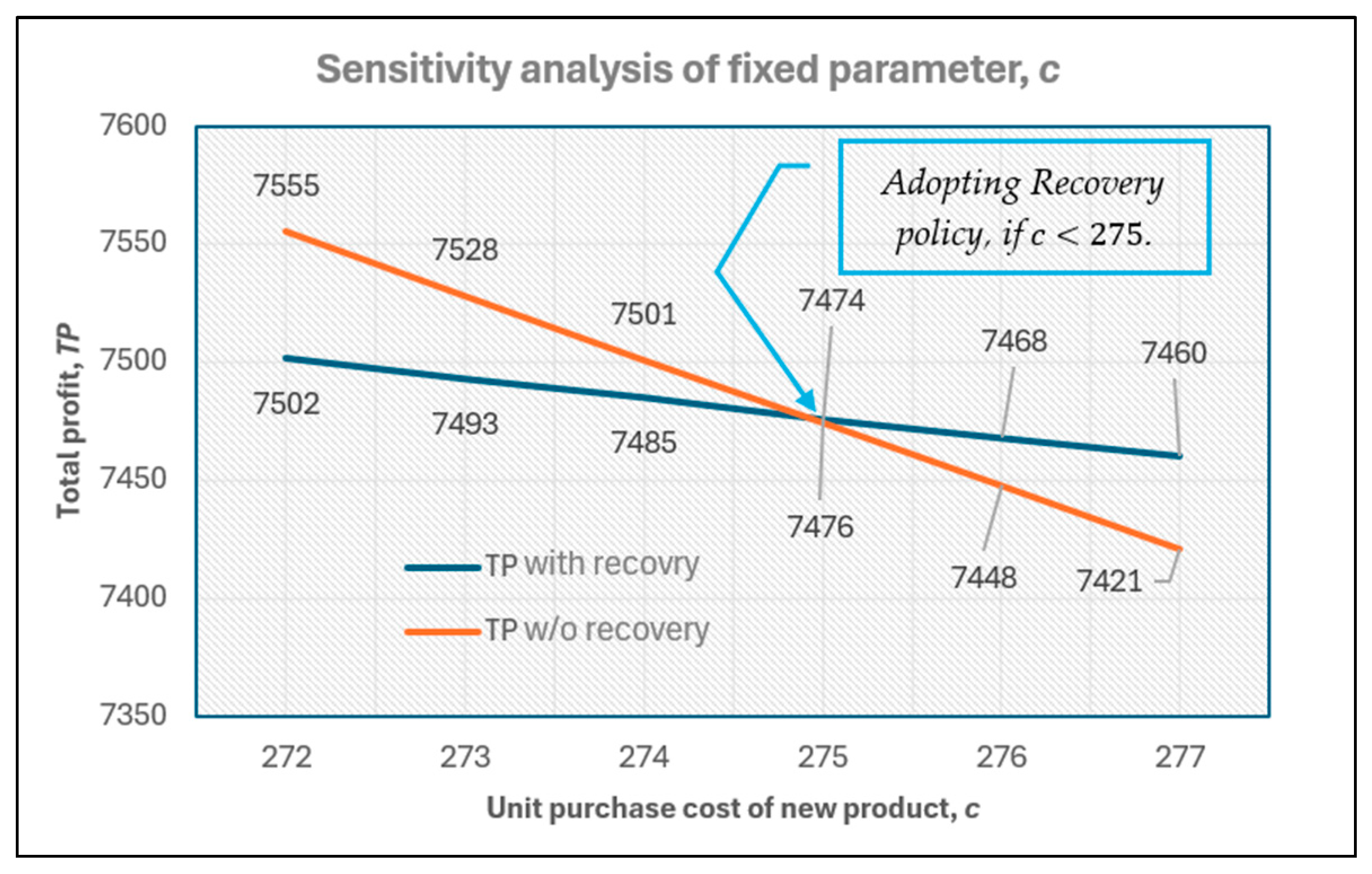
An increase in purchase cost (c) leads to a higher selling price and a smaller lot size (Q) (see Table 8 and Figure 7), since the higher selling price reduces demand (D), which in turn decreases lot size (Q). Figure 8 compares the total profit with and without recovery under different purchase costs (c). A critical threshold emerges: when the purchase cost is below this threshold, recovery yields less total profit than no recovery. Conversely, when the purchase cost exceeds this value, recovery becomes more profitable. Table 8 and Figure 8 show that when the purchase cost is below USD 275, recovery is not worth considering, whereas it becomes beneficial once the purchase cost reaches or surpasses this value.
Table 8. Sensitivity analysis of new-product unit purchase cost c.
Policy c P T TP TC SR Q Q r PTPC (%)
With recovery363609.30.35216794803714,7908.5945.765−3.2
346.5605.90.35216886797714,8638.6385.795−1.9
{330}602.50.35037020791414,9348.6825.8250.0
313.5599.10.34847155784915,0048.7265.8551.9
297595.70.34667292778115,0738.7705.8843.9
277591.60.34457460769515,1548.8235.9206.3
276591.40.34447468769015,1588.8265.9226.4
275591.20.34437476768615,1628.8285.9246.5
274591.00.34427485768115,1668.8315.9266.6
273590.80.34407493883415,1708.8345.9286.7
272590.60.34397502883615,1748.8365.9296.9
Without recovery277649.80.33277421985717,2798.847NA5.7
276649.20.33237448984917,2978.855NA6.1
275648.60.33207474984017,3158.863NA6.5
274648.00.33167501983217,3338.871NA6.9
273647.30.33137528982317,3518.879NA7.2
272646.70.33097555888717,3698.887NA7.6
Note: Basic column; percentage of total profit change (PTPC) = T P T P / T P . NA: Not available.
Figure 7. Unit sale price and lot size vs. c.
Mathematics 13 02916 g007
Figure 8. Total profit vs. c for both policies, with and without recovery. Summary: With the unit purchase cost of a new product, TP decreases when c increases, both with and without the recovery policy. In addition, if the recovery rate c < 275 , it is worth choosing the recovery policy.
Mathematics 13 02916 g008
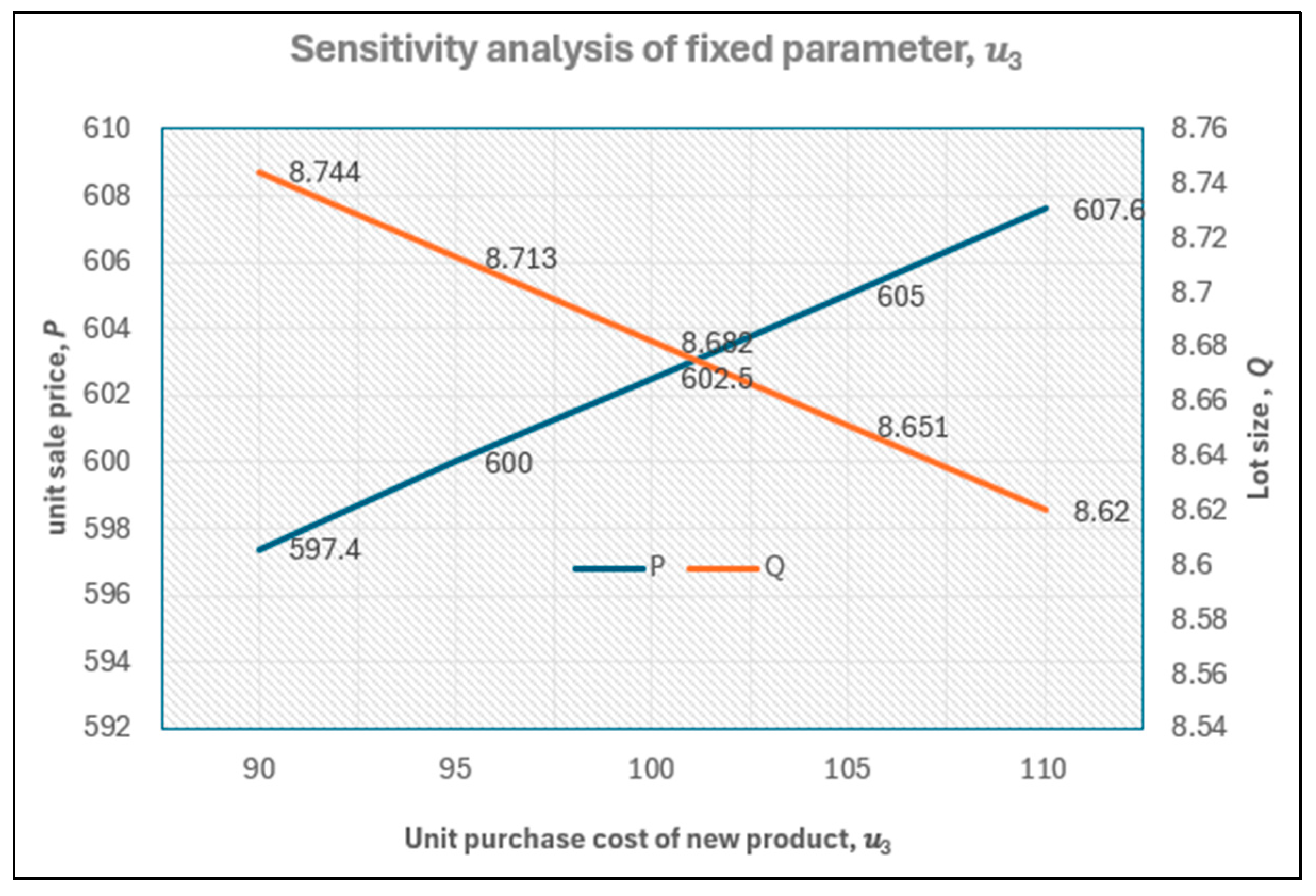
When the purchase cost for used products ( u 3 ) increases, the selling price increases and the lot size (Q) decreases (see Table 9 and Figure 9). Figure 10 compares the total profit with and without recovery when the purchase cost of used products ( u 3 ) varies, as shown in Table 9. When the purchase cost reaches or exceeds the critical value of USD 149, it is not worthwhile to consider recovery; however, if the cost is lower than this value, recovery is worthwhile.
Table 9. Sensitivity analysis of unit purchase cost of used product u 3 .
u 3 PTTPTCSR Q Q r PTPC (%)
151628.40.36606048830814,3568.3615.606−13.8
150627.90.36576067830214,3688.3675.610−13.6
149627.40.36536085829514,3808.3745.614−13.3
148626.90.36506103828914,3928.3805.619−13.1
147626.40.36476122828314,4048.3865.623−12.8
146625.90.36446140827614,4168.3935.628−12.5
110607.60.35326823800414,8278.6205.782−2.8
105605.00.35176921796014,8818.6515.804−1.4
{100}602.50.35037020791414,9348.6825.8250.0
95600.00.34887120786714,9878.7135.8461.4
90597.40.34747220781915,0398.7445.8672.8
Note: Basic column; percentage of total profit change (PTPC) = T P T P / T P .
Figure 9. Unit sale price and lot size vs. u 3 .
Mathematics 13 02916 g009
Figure 10. Total profit vs. u 3 for both policies, with and without recovery. Summary: With the unit purchase cost for used products, TP decreases when u 3 increases, but only with the recovery policy applied. In addition, if the recovery rate u 3 < 149 , it is worth choosing the recovery policy.
Mathematics 13 02916 g010
As shown in Table 10, a higher yield rate (f) of recovery results in a lower selling price, a larger lot size, and a greater total profit. This creates a win–win outcome for both consumers and the entire supply chain. The relationship between total profit and yield rate with and without recovery is shown in Figure 11. When the yield rate of recovery is equal to or higher than the critical yield rate value, 0.70, it is worth considering recovery; conversely, it is not worth considering when the yield rate is equal to or lower than 0.69.
Table 10. Sensitivity analysis of yield rate f.
fPTTPTCSR Q Q r PTPC (%)
0.935586.30.34037569754215,1118.7716.4947.8
0.8925594.40.34527291773515,0268.7276.1573.9
{0.850}602.50.35037020791414,9348.6825.8250.0
0.8075610.60.35556755808014,8358.6375.496−3.8
0.765618.70.36096496823214,7288.5925.170−7.5
0.720627.30.36696228837914,6078.5434.829−11.3
0.710629.20.36826169840914,5798.5324.754−12.1
0.700631.10.36966111843914,5508.5214.679−12.9
0.690633.00.37096053846814,5218.5104.604−13.8
0.680634.90.37235996849614,4928.4994.530−14.6
0.670636.80.37375938852414,4628.4884.455−15.4
Note: Basic column; percentage of total profit change (PTPC) = T P T P / T P .
Figure 11. Total profit vs. f for both policies, with and without recovery. Summary: With the yield rate from recovery, TP increases as f increases, but only under the recovery policy. Moreover, if the recovery rate satisfies f 0.70 , adopting the recovery policy is worthwhile.
Mathematics 13 02916 g011
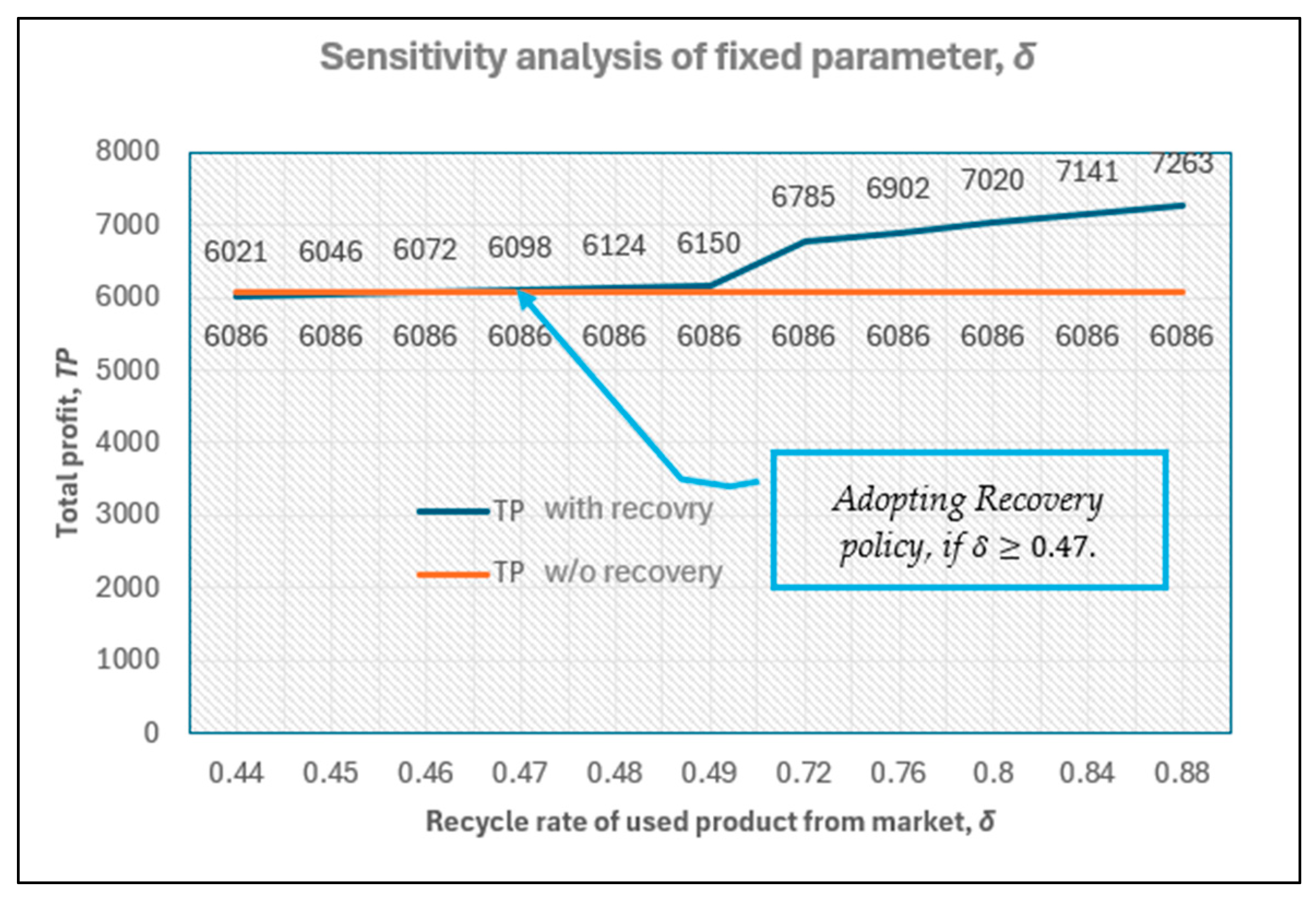
From Table 11 and Figure 12, an increasing recycling rate (δ) results in a greater lot size (Q) and total profit. When the recycling rate of used products is equal to or higher than the critical recycling rate value of 0.47, adopting recovery is worthwhile; conversely, if the rate is equal to or lower than 0.46, recovery is not worthwhile. The relationship patterns between the total profit and the parameters of the recycling rate and yield rate are identical.
Table 11. Sensitivity analysis of recycling rate δ.
δPTTPTCSR Q Q r PTPC (%)
0.88593.90.34457263770214,9648.6806.4253.5
0.84598.20.34737141781014,9508.6816.1241.7
{0.8}602.50.35037020791414,9348.6825.8250.0
0.76606.80.35336902801614,9178.6845.526−1.7
0.72611.10.35636785811314,8988.6875.229−3.3
0.49635.50.37536150861014,7608.7173.536−12.4
0.48636.60.37626124862914,7538.7183.463−12.8
0.47637.60.37716098864814,7468.7203.390−13.1
0.46638.70.37806072866714,7398.7223.317−13.5
0.45639.70.37896046868514,7318.7243.244−13.9
0.44640.80.37986021870314,7248.7273.171−14.2
Note: Basic column; percentage of total profit change (PTPC) = T P T P / T P .
Figure 12. Total profit vs. δ for both policies with and without recovery. Summary: With the recycling rate, TP increases as δ increases, but only under the recovery policy. In addition, if the recovery rate δ 0.47 , adopting the recovery policy is worthwhile.
Mathematics 13 02916 g012

Discussion of Key Cost-Based Parameters

As indicated in Table 8, Table 9, Table 10 and Table 11 and Figure 8, Figure 10, Figure 11 and Figure 12, the relationship between the total profit and cost-based parameters in the set Φ2 = {c, u 3 , f, δ} is revealed when recovery is considered. The set Φ2 represents key parameters associated with cost or profit. Managers can use these indicators to make quick decisions on whether to adopt a recovery policy.

6. Concluding Remarks

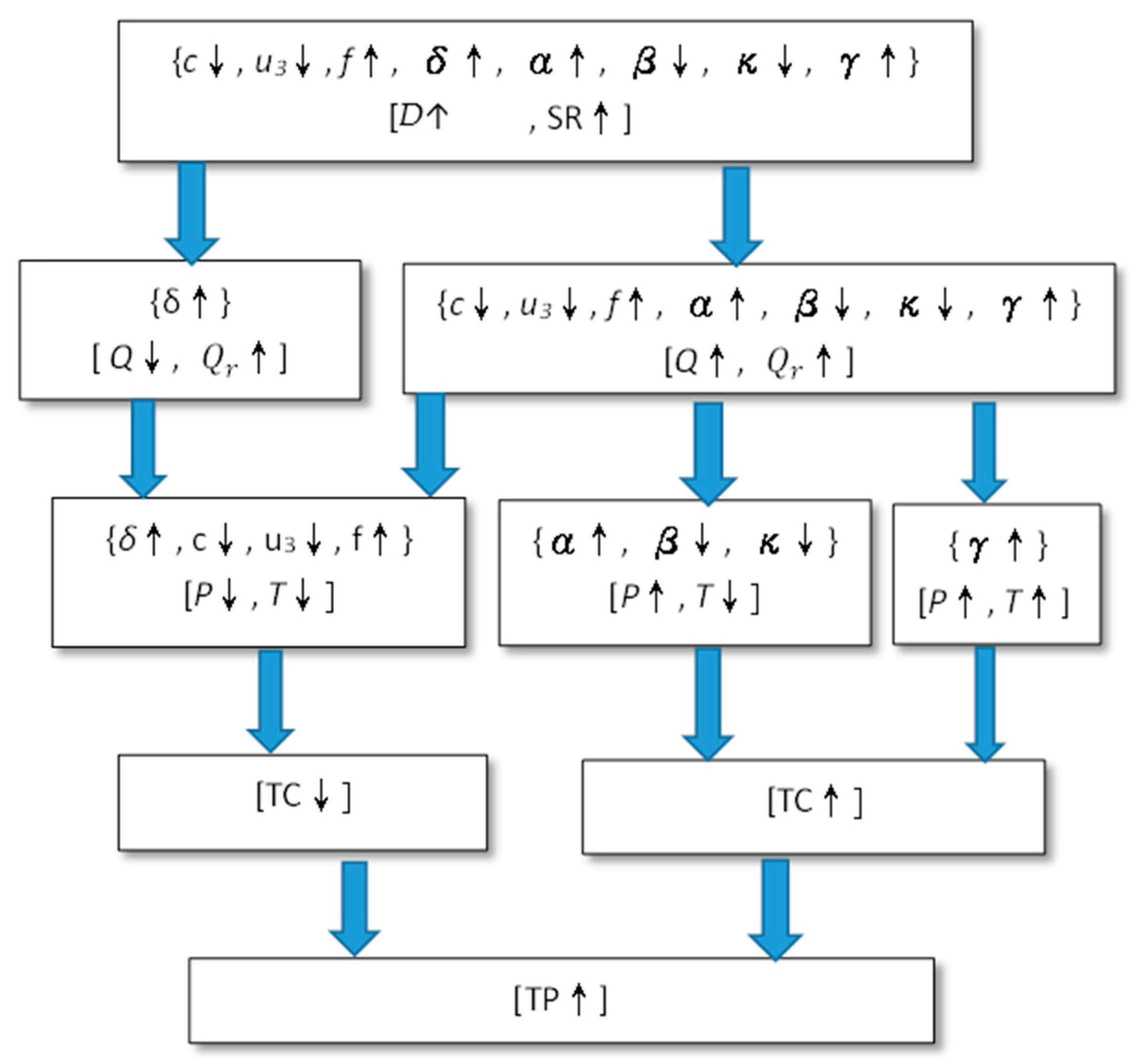
Unlike existing models, this study proposes an EOQ model with recovery, incorporating demand sensitivity to price, stock, and carbon emissions. The impact on recovery is comprehensively examined through sensitivity analysis. The following observations are made: (i) The recovery mechanism increases the total profit by approximately 15%. (ii) The primary reason for this increase is the reduction in purchase cost (−40%), rather than an increase in the selling price (see Table 3). (iii) The recovery mechanism benefits both the seller and consumer, resulting in a higher seller profit (+15%) and lower selling price (−12%), rather than benefiting only the seller. (iv) A critical unit purchase cost exists; if the unit purchase cost is lower than this value, it is not worth considering recovery. However, if the unit purchase cost exceeds this critical value, recovery is worth considering. Similar thresholds exist for other parameters, such as the recycling rate, yield rate, and unit purchase cost of used products. In other words, recovery is advantageous only if c ≥ 275, u 3 < 149, f ≥ 0.70, or δ ≥ 0.47 (please see Figure 8, Figure 10, Figure 11 and Figure 12). (v) In most cases, higher profit requires higher input costs. However, for budget-constrained enterprises, a unique solution is to adopt a recovery mechanism to achieve higher profits with lower costs (refer to Figure 13).

6.1. The Parameter Relationship Map

Based on Table 4, Table 5, Table 6, Table 7, Table 8, Table 9, Table 10 and Table 11, the relationship between parameters ( c , u 3 , f , δ , α , β , k , and γ ) and decision variables (P, T, Q , Q r , SR, TC, TP, PTPC) can be represented as a map, as shown in Figure 13.
By adjusting purchase cost and recovery-related parameters (c↓, u 3 ↓, f↑, δ ↑), the seller can simultaneously reduce cost and increase profit, while the consumer pays a lower price. Conversely, changes in non-recovery-related parameters ( α ↑, β ↓, k ↓, γ ↑) may increase seller profit, but at the expense of higher costs and higher consumer prices.

6.2. Managerial Implications, Limitations, Application and Future Research

The managerial implications of this study highlight the need for a shift in inventory management practices toward a more holistic approach that integrates sustainability into decision-making. By optimizing an inventory model that considers limited recovery rates and demand sensitivity to price, carbon emissions, and stock conditions, managers can better align their operations with both economic and environmental goals. When recovery is considered, the total profit increases by 15%, while the total cost decreases by 22% compared with the case without recovery, mainly because the purchase cost is 40% lower. Other contributing factors include a 12% reduction in the selling price and a 4% increase in demand. This represents a win–win policy for both sellers and consumers: consumers can buy products at lower prices (−12%), while sellers can sell more products (+4%) and earn higher profit (+15%). Adopting such an approach can lead to improved long-term profitability, compliance with regulatory standards, and a competitive edge in markets that are increasingly driven by sustainability considerations.
The model limitations, data, and application constraints, and directions for research and industrial application are summarized as follows:
  • The assumption of synchronized cycle times for EOQ and recovery may limit real-world applicability. Relaxing this assumption improves practical applicability but increases the complexity of the analytical framework. Section 1 discusses this effect.
  • To address the data/application constraints of optimizing the proposed sustainable inventory model, further explanation is needed to enhance the model’s applicability and validity in practice.
  • A critical area for future research is the integration of stochastic elements to account for uncertainties in recovery rates, demand fluctuations, and supply chain disruptions, thereby strengthening the model’s performance under real-world conditions. Additionally, incorporating multi-objective optimization techniques could balance conflicting goals, such as minimizing carbon emissions while maximizing profit, thereby providing more comprehensive decision-making tools for managers. Expanding the model to consider circular economic principles, such as the reuse and recycling of materials, could further enhance its sustainability impact.
  • Future studies could also investigate the effects of different regulatory environments, such as varying carbon pricing mechanisms or environmental standards, on inventory decisions. This would provide valuable insights into how companies can effectively strategize across various regions. Another promising direction involves expanding the model to include multi-echelon supply chains, where sustainability considerations are coordinated across multiple layers of suppliers and distributors [33]. Finally, the exploration of policy implications, such as the effects of carbon taxes or subsidies on inventory decisions, could provide valuable insights for both managers and policymakers seeking to balance economic and environmental objectives [34].

Author Contributions

Conceptualization, J.C.-P.Y.; Methodology, X.-B.L.; Validation, X.-B.L. and J.-M.C.; Formal analysis, X.-B.L., J.C.-P.Y. and J.-M.C.; Investigation, J.C.-P.Y.; Resources, J.-M.C.; Data curation, X.-B.L.; Writing—original draft, X.-B.L.; Writing—review & editing, J.-M.C.; Visualization, X.-B.L.; Project administration, J.C.-P.Y.; Funding acquisition, J.C.-P.Y. All authors have read and agreed to the published version of the manuscript.

Funding

National Science and Technology Council, Taiwan, NSTC 114-2410-H-147-001-MY2.

Data Availability Statement

The original contributions presented in this study are included in the article. Further inquiries can be directed to the corresponding author.

Acknowledgments

The authors would like to thank the Editor-in-Chief and the anonymous reviewers for their helpful comments and suggestions. The funding from the National Science and Technology Council, Taiwan, under research grant NSTC 114-2410-H-147-001-MY2 is greatly appreciated.

Conflicts of Interest

The authors declare no conflicts of interest.

Appendix A. Taylor’s Series Expansion

Using Taylor’s series expansion, e y can be approximated by 1 + y + 1 2 ! y 2 if y 1 .
The error percentage is 1 3 ! y 3 1 + y + 1 2 ! y 2 + 1 3 ! y 3 . When γ · T = 0.15 , the error percentage is 0.0484%. It can be neglected for anything higher than the third terms in Equations (5)–(7).

Appendix B. The Proof of Global Optimality

Assume there is a real-valued function f ( x 1 ,   x 2 ,   ,   x n ) with second-order partial derivatives that are continuous in the domain of definition. Then, the Hessian matrix of the function f is
H ( x ˜ ) = 2 f ( x ˜ ) x 1 2 2 f ( x ˜ ) x 1 x 2 2 f ( x ˜ ) x 1 x n 2 f ( x ˜ ) x 2 x 1 2 f ( x ˜ ) x 2 2 2 f ( x ˜ ) x 2 x n 2 f ( x ˜ ) x n x 1 2 f ( x ˜ ) x n x 2 2 f ( x ˜ ) x n 2
Hence, let det[H(P, T)] be the determination of H(P, T), where matrix H(P, T) is known as the Hessian Matrix of TP(P, T) at (P, T). For the function to be concave, the following sufficient conditions must be satisfied, d e t [ H P , T ] < 0 , provided that
T P P , T P = 0 ,   T P P , T T = 0
T P P , T P = 0 , T P P , T T = 0
2 T P ( P , T ) P 2 < 0   o r   2 T P ( P , T ) T 2 < 0
and
2 T P ( P , T ) P 2 2 T P ( P , T ) T 2 T P P , T P T P P , T T 2 > 0
The result obtained from applying the above solution procedure to this example is {P = 602.5, T = 0.3503}. The results of calculating the above conditions are as follows: 2 T P ( P , T ) P 2 = 0.15 < 0 , 2 T P ( P , T ) T 2 = 98919 < 0 , and 2 T P ( P , T ) P 2 2 T P ( P , T ) T 2 T P P , T P T P P , T T 2 = 11862 > 0 . Therefore, this solution is optimal.

References

  1. Dwicahyani, A.R.; Kholisoh, E.; Rosyidi, C.N.; Laksono, P.W.; Jauhari, W.A. Inventory model optimization for a closed-loop retailer-manufacturer-supplier system with imperfect production, reworks and quality dependent return rate. Int. J. Serv. Oper. Manag. 2020, 35, 528–556. [Google Scholar]
  2. Mahato, C.; Mahata, G.C. Sustainable partial backordering inventory model under linked-to-order credit policy and all-units discount with capacity constraint and carbon emissions. Flex. Serv. Manuf. J. 2023, 35, 896–944. [Google Scholar] [CrossRef]
  3. Feng, G.F.; Long, H.; Wang, H.J.; Chang, C.P. Environmental, social and governance, corporate social responsibility, and stock returns: What are the short-and long-Run relationships. Corp. Soc. Responsib. Environ. Manag. 2022, 29, 1884–1895. [Google Scholar] [CrossRef]
  4. Khouja, M. Synchronization in supply chains: Implications for design and management. J. Oper. Res. Soc. 2003, 54, 984–994. [Google Scholar] [CrossRef]
  5. Yu, C.P.; Yang, P.C.; Lai, X.C. Integrated manufacturer-retailer closed-loop inventory system with price-sensitive return and demand rates. J. Ind. Prod. Eng. 2019, 36, 134–145. [Google Scholar] [CrossRef]
  6. Hasan, S.M.; Mashud, A.H.M.; Miah, S.; Daryanto, Y.; Lim, M.K.; Tseng, M.L. A green inventory model considering environmental emissions under carbon tax, cap-and-offset, and cap-and-trade regulations. J. Ind. Prod. Eng. 2023, 40, 538–553. [Google Scholar] [CrossRef]
  7. Mabini, M.C.; Pintelon, L.M.; Gelders, L.F. EOQ type formulation for controlling repairable inventories. Int. J. Prod. Econ. 1992, 28, 21–33. [Google Scholar] [CrossRef]
  8. Wee, H.M. Joint pricing and replenishment policy for deteriorating inventory with declining market. Int. J. Prod. Econ. 1995, 40, 163–171. [Google Scholar] [CrossRef]
  9. Giri, B.C.; Chaudhuri, K.S. Deterministic models of perishable inventory with stock-dependent demand rate and nonlinear holding cost. Eur. J. Oper. Res. 1998, 105, 467–474. [Google Scholar] [CrossRef]
  10. Teng, J.T.; Chang, C.T. Economic production quantity models for deteriorating items with price- and stock-dependent demand. Comput. Oper. Res. 2005, 32, 297–308. [Google Scholar] [CrossRef]
  11. Shaikh, A.A.; Mashud, A.H.M.; Uddin, M.S.; Khan, M.A.A. Non-instantaneous deterioration inventory model with price and stock dependent demand for fully backlogged shortages under inflation. Int. J. Bus. Forecast. Mark. Intell. 2017, 3, 152–164. [Google Scholar] [CrossRef]
  12. Schrady, D.A. A deterministic inventory model for repairable items. Nav. Res. Logist. Q. 1967, 14, 391–398. [Google Scholar] [CrossRef]
  13. Nahmias, S.; Rivera, H. A deterministic model for a repairable item inventory system with a finite repair rate. Int. J. Prod. Res. 1979, 17, 215–221. [Google Scholar] [CrossRef]
  14. Koh, S.G.; Hwang, H.; Sohn, K.I.; Ko, C.S. An optimal ordering and recovery policy for reusable items. Comput. Ind. Eng. 2002, 43, 59–73. [Google Scholar] [CrossRef]
  15. Maity, S.; Chakraborty, A.; De, S.K.; Pal, M. A study of an EOQ model of green items with the effect of carbon emission under pentagonal intuitionistic dense fuzzy environment. Soft Comput. 2023, 27, 15033–15055. [Google Scholar] [CrossRef]
  16. Khan, M.A.A.; Cárdenas-Barrón, L.E.; Treviño-Garza, G.; Céspedes-Mota, A.; de Jesús Loera-Hernández, I. Integrating prepayment installment, pricing and replenishment decisions for growing items with power demand pattern and non-linear holding cost under carbon regulations. Comput. Oper. Res. 2023, 156, 106225. [Google Scholar] [CrossRef]
  17. Hua, G.; Cheng, T.C.E.; Wang, S. Managing carbon footprints in inventory management. Int. J. Prod. Econ. 2011, 132, 178–185. [Google Scholar] [CrossRef]
  18. Inderfurth, K.; Lindner, G.; Rachaniotis, N.P. Lot sizing in a production system with rework and product deterioration. Int. J. Prod. Res. 2005, 43, 1355–1374. [Google Scholar] [CrossRef]
  19. Chung, S.L.; Wee, H.M.; Yang, P.C. Optimal policy for a closed-loop supply chain inventory system with remanufacturing. Math. Comput. Model. 2008, 48, 867–881. [Google Scholar] [CrossRef]
  20. Yang, P.C.; Wee, H.M.; Chung, S.L.; Ho, P.C. Sequential and global optimization for a closed-loop deteriorating inventory supply chain. Math. Comput. Model. 2010, 52, 161–175. [Google Scholar] [CrossRef]
  21. Hovelaque, V.; Bironneau, L. The carbon-constrained EOQ model with carbon emission dependent demand. Int. J. Prod. Econ. 2015, 164, 285–291. [Google Scholar] [CrossRef]
  22. Helmrich, M.J.R.; Jans, R.; Heuvel, W.D.; Wagelmans, A.P.M. The economic lot-sizing problem with an emission capacity constraint. Eur. J. Oper. Res. 2015, 241, 50–62. [Google Scholar] [CrossRef]
  23. Ghosh, A.; Jha, J.K.; Sarmah, S.P. Optimal lot-sizing under strict carbon cap policy considering stochastic demand. Appl. Math. Model. 2017, 44, 688–704. [Google Scholar] [CrossRef]
  24. Aljuneidi, T.; Bulgak, A.A. Carbon footprint for designing reverse logistics network with hybrid manufacturing-remanufacturing systems. J. Remanuf. 2020, 10, 107–126. [Google Scholar] [CrossRef]
  25. Chan, C.K.; Man, N.; Fang, F.; Campbell, J.F. Supply chain coordination with reverse logistics: A vendor/recycler-buyer synchronized cycles model. Omega 2020, 95, 102090. [Google Scholar] [CrossRef]
  26. Konstantaras, I.; Skouri, K.; Benkherouf, L. Optimizing inventory decisions for a closed-loop supply chain model under a carbon tax regulatory mechanism. Int. J. Prod. Econ. 2021, 239, 108185. [Google Scholar] [CrossRef]
  27. Sarkar, B.; Guchhait, R. Ramification of information asymmetry on a green supply chain management with the cap-trade, service, and vendor-managed inventory strategies. Electron. Commer. Res. Appl. 2023, 60, 101274. [Google Scholar] [CrossRef]
  28. Rahman, M.S.; Rahman, M.J.; Al-Habsi, N. Hygienic design and sanitation. In Handbook of Food Preservation; CRC Press: Boca Raton, FL, USA, 2020; pp. 957–968. [Google Scholar]
  29. Liu, M.; Fang, S.; Dong, H.; Xu, C. Review of digital twin about concepts, technologies, and industrial applications. J. Manuf. Syst. 2021, 58, 346–361. [Google Scholar] [CrossRef]
  30. Sarkar, B.; Bhuniya, S. A sustainable flexible manufacturing–remanufacturing model with improved service and green investment under variable demand. Expert Syst. Appl. 2022, 202, 117154. [Google Scholar] [CrossRef]
  31. Lin, J.; Naim, M.; Tang, O. In-house or outsourcing? The impact of remanufacturing strategies on the dynamics of component remanufacturing systems under lifecycle demand and returns. Eur. J. Oper. Res. 2024, 315, 965–979. [Google Scholar] [CrossRef]
  32. Sebatjane, M. Sustainable inventory models under carbon emissions regulations: Taxonomy and literature review. Comput. Oper. Res. 2025, 173, 106865. [Google Scholar] [CrossRef]
  33. Xu, Z.; Pokharel, S.; Elomri, A. An eco-friendly closed-loop supply chain facing demand and carbon price uncertainty. Ann. Oper. Res. 2023, 320, 1041–1067. [Google Scholar] [CrossRef]
  34. Li, J.; Lai, K.K.; Li, Y. Remanufacturing and low-carbon investment strategies in a closed-loop supply chain under multiple carbon policies. Int. J. Logist. Res. Appl. 2024, 27, 170–192. [Google Scholar] [CrossRef]
  35. Spiegel, M.R. Applied Differential Equations, Englewood Cliffs; Prentice Hall: Upper Saddle River, NJ, USA, 1960. [Google Scholar]
Figure 1. The flow of a mixed production system.
Mathematics 13 02916 g001
Figure 2. Total profit with respect to P and T (with recovery policy). Note: This figure shows a concave function TP, where the optimal set {P = 602.5, T = 0.3503}.
Mathematics 13 02916 g002
Figure 13. Map of various decisions made while changing known parameters. Note: ↑: increase; ↓: decrease.
Mathematics 13 02916 g013
Table 1. Comparison between the proposed work and previous studies.
ReferenceCarbon
Emission
ESGRecovery
Operations
Sustainability
[1]NoNoYesYes
[2]YesNoYesNo
[3]YesNoNoNo
[5]NoYesYesNo
[6]YesNoYesNo
[7]NoYesNoYes
[8]NoNoNoYes
[9]NoNoNoYes
[10]NoNoNoYes
[11]NoNoNoYes
[12]NoYesYesYes
[13]NoYesYesYes
[14]NoYesYesYes
[15]YesNoYesYes
[16]NoNoNoYes
[17]YesNoNoYes
[18]NoYesNoYes
[19]NoNoYesYes
[20]NoNoYesYes
[21]YesNoYesYes
[22]YesNoNoYes
[23]YesNoNoYes
[24]YesYesNoNo
[25]NoNoYesYes
[26]YesNoYesYes
[27]YesNoNoYes
[30]NoNoYesYes
[31]YesYesYesNo
[32]YesNoYesYes
[33]YesNoYesNo
[34]YesNoYesYes
Proposed modelYesYesYesYes
Table 2. Notations.
Table 2. Notations.
The demand-based parameters
DAnnual demand rate, where D = α β P κ E + γ I ( t ) .
αFixed demand parameter
βPrice-sensitive parameter
EAnnual carbon emissions including production process (Ec) and recovery process (Er)
κCarbon-emission-sensitive parameter
γStock-dependent parameter
The cost-based parameters
SSetup cost per cycle
HHolding cost per unit per year
cUnit purchase cost of new product
u 1 Unit carbon tax
u 2 Unit carbon trading price
u 3 Unit purchase cost for used product from market
u 4 Unit disposal cost for each recovery scrap
Others
I(t)Inventory level with time
S c Carbon emissions per setup
H c Carbon emissions for each holding unit per year
S r Recovery setup cost per cycle
H r Recovery holding cost per unit per year
S r c Recovery carbon emissions per setup
H r c Recovery carbon emissions per holding unit per year
ZCarbon credit
δ Recycle rate of used product from market, 0 < δ < 1
f Yield rate from recovery, 0 < f < 1
The decision variables
TCycle time
PUnit sales price for each finished product
The dependent variables
Q Lot size during a given cycle time
Q r Used product recovered during a given cycle time
TPAnnual total profit denoted as TP(P, T)
Table 3. Comparison between including and excluding recovery policy.
PolicyWith Recovery (i)Without Recovery (ii) Difference = i     i i i i   ( % )
Optimal Results
Total profit, T P   7020608615%
Total cost, TC791410,162−22%
Sales revenue, SR14,93416,247−8%
Purchase cost, PC46757857−40%
Scrap disposal cost, SDC1490NA
Classical cost, CC136113362%
Recovery cost, RC2990NA
Carbon emission cost, CEC143196948%
Selling price, P   602.5682.4−12%
Cycle time, T   0.35030.3532−1%
Lot size, Q   8.6828.4093%
Recovery lot size, Q r   5.8250NA
Note: * means the optimal solution; NA: not available.
Disclaimer/Publisher’s Note: The statements, opinions and data contained in all publications are solely those of the individual author(s) and contributor(s) and not of MDPI and/or the editor(s). MDPI and/or the editor(s) disclaim responsibility for any injury to people or property resulting from any ideas, methods, instructions or products referred to in the content.