Abstract
Accurate prediction of a robot’s dynamic parameters, including mass and moment of inertia, is essential for adequate motion planning and control in autonomous systems. Traditional methods often depend on manual computation or physics-based modelling, which can be time-consuming and approximate for intricate, real-world environments. Recent advances in machine learning, primarily through artificial neural networks (ANNs), offer profitable alternatives. However, the potential of quantum-inspired models in this context remains largely uncharted. The current research assesses the predictive performance of a classical artificial neural network (CANN) and a quantum-inspired artificial neural network (QANN) in estimating a car-like mobile robot’s mass and moment of inertia. The predictive accurateness of the models was considered by minimizing a cost function, which was characterized as the RMSE between the predicted and actual values. The outcomes indicate that while both models demonstrated commendable performance, QANN consistently surpassed CANN. On average, QANN achieved a 9.7% reduction in training RMSE, decreasing from 0.0031 to 0.0028, and an 84.4% reduction in validation RMSE, dropping from 0.125 to 0.0195 compared to CANN. These enhancements highlight QANN’s singular predictive accuracy and greater capacity for generalization to unseen data. In contrast, CANN displayed overfitting tendencies, especially during the training phase. These findings emphasize the significance of quantum-inspired neural networks in enhancing prediction precision for involved regression tasks. The QANN framework has the potential for wider applications in robotics, including autonomous vehicles, uncrewed aerial vehicles, and intelligent automation systems, where accurate dynamic modelling is necessary.
Keywords:
car-like robot; quantum computing; artificial neural network; hybrid activation functions; quantum artificial neural network; dynamic parameter estimation MSC:
34A34; 68T07; 03G12
1. Introduction
1.1. Context of the Study
Over the past decade, mobile robotics has experienced remarkable advancements, mainly driven by an increasing demand for intelligent autonomy, resilient adaptability, and context-sensitive decision-making. Nowadays, these systems are essential for required applications across various fields, such as autonomous driving, industrial logistics, planetary exploration, and precision agriculture. A key requirement for ensuring the performance, reliability, and safety of mobile robots, particularly wheeled platforms constrained by nonholonomic conditions, is the accurate characterization of their underlying dynamics. In practice, this necessitates the precise identification of essential physical parameters, including effective mass, inertia distribution, and other mechanical properties. These parameters play an important role in controlling the stability of motion control algorithms, the efficiency of trajectory planning, and the overall active performance of the system, making the dynamic modeling and parameter estimation critical components of advanced mobile robotic design [1,2,3].
Parameter identification of dynamic systems traditionally depended on physics-based dynamic models, which require detailed prior knowledge of a robot’s kinematic structure, mass distribution, and payload characteristics. While such formulations can be effective under well-defined laboratory conditions, they often involve considerable computational effort and limited adaptability, rendering them vulnerable to modeling errors and unmodeled dynamics. Their dependence on precise geometric and inertial information makes them especially delicate in the presence of environmental uncertainties or nonlinear interactions. In practical deployments, such as handling variable payloads on irregular terrains, these limitations often manifest as degraded tracking precision, increased control demands, and reduced resilience to external disturbances [4,5,6].
Data-driven approaches, and, in particular, artificial neural networks (ANNs), have increasingly been recognized as powerful alternatives to conventional model-based strategies. Unlike rigid physical modeling, ANNs can capture intricate nonlinear dynamics by providing a flexible and scalable framework for adaptive system identification. When ANNs are utilized for dynamic parameter estimation, they are capable of extracting latent patterns from trajectory data that often remain inaccessible to standard identification techniques. Nonetheless, conventional ANN architectures are not without limitations: they are prone to overfitting, exhibit strong dependence on large volumes of high-quality data, and frequently struggle to generalize effectively in environments characterized by noise or sparse sampling [7,8,9]. The identified gap highlights the necessity of developing novel modeling strategies capable of preserving the flexibility of artificial neural networks while improving stability and data-efficiency, with a special emphasis on accurate parameter estimation essential to the real-time functionality of mobile robotic systems.
1.2. Related Works
While classical artificial neural networks have contributed to robotic modeling and control advancements, several challenges remain. These models often require large datasets, are prone to overfitting, and may struggle with generalization in dynamic, unstructured environments. Furthermore, traditional techniques for estimating parameters such as mass and inertia are embedded in specified physics, making them computationally intensive and less adaptable to the complexities of real-world robotic systems.
To address this gap, the present study implements and evaluates two artificial neural network architectures: a classical neural network and a quantum-inspired neural network. These models are developed to predict a mobile robot’s mass and moment of inertia designated on trajectory-based error metrics. Both models were trained to estimate dynamic parameters crucial for accurate motion control using a dataset consisting of the root mean square error values between the desired and actual trajectories. The study aims to consider the comparative performance of these architectures with respect to prediction accuracy and generalization capabilities. The conclusions indicate that the QANN outperforms the CANN in reducing training and validation errors, demonstrating superior learning capability and robustness. The study contributes to the field by showcasing the practical applicability of quantum-inspired neural networks for regression tasks in robotic modeling, underlining their possibility to enhance real-time control in autonomous systems.
Artificial neural networks have appeared as potent tools in mobile robotics, significantly enhancing critical areas such as real-time decision-making, perception, and control. Their capacity for nonlinear relationships makes them especially well-suited for dynamic conditions and autonomous operations. Numerous studies have confirmed the practical applications of ANNs in improving various robotic functionalities. Wang et al. [10] proposed an end-to-end approach for trajectory planning and motion control utilizing deep reinforcement learning (DRL). By developing a physical model of the robot and optimizing LiDAR inputs, their method processed obstacle distances, enhancing obstacle avoidance and overall adaptability. This research underlines the importance of integrating sensor data with neural control frameworks to improve autonomous navigation. Mutti et al. [11] introduced a recurrent neural network RNN-based algorithm to reduce the computational demands commonly associated with modeling autonomous robots. Their strategy involved training the model on synthetic data and augmenting LiDAR signals through rigid transformations. The model was subsequently fine-tuned using real-world positional data and external camera measurements. This hybrid training approach eased the need for extensive real-world datasets, addressing a standard limitation of robotics-based deep learning methods. Ding et al. [12] presented a tracking control algorithm based on partial reinforcement learning neural networks in another contribution. Their strategy particularly tackled the challenge of trajectory tracking in wheeled mobile robots with time-varying feed angles. Their model showed enhanced adaptability in managing nonlinear and uncertain trajectory patterns by utilizing partial reinforcement signals. Also analyzing hybrid strategies, a study [13] combined maneuver classification through standard neural networks with trajectory prediction using long short-term memory (LSTM) networks. This dual-layered model aimed to enhance vehicle localization and future position estimation. Combining temporal dependencies via LSTM networks proved beneficial in predicting complicated, dynamic motion patterns. Hu et al. [14] addressed efficiency and energy consumption in multi-robot systems through a cooperative exploration strategy. They implemented dynamic Voronoi partitions to minimize redundant area coverage while integrating a deep reinforcement learning (DRL)-based collision avoidance algorithm for navigation in dynamic and uncertain environments. Their method allowed real-time obstacle detection and interaction prediction, essential capabilities for practical deployment. Several studies have supported employing optimized deep-learning architectures for object detection to promote efficient perception. Studies such as [15,16] employed algorithms like Faster R-CNN, R-FCN, and SSD to balance detection accuracy, computational speed, and memory utilization, especially within autonomous driving.
Despite these advancements, multi-object detection and tracking challenges persist in problematic traffic scenarios. Ravindran et al. [17] handled these challenges through data fusion and sensor integration. Their work underscored the matter of integrating spatial and temporal data streams, enhancing the reliability of real-time object tracking across diverse situations. Huang et al. [18] also improved autonomous driving performance with a deep learning model that utilized multimodal sensor fusion. By merging RGB images and depth data at an early fusion stage, they performed detailed per-pixel semantic segmentation, thus enhancing environmental performance and control accuracy. Lio et al. [19] introduced an innovative artificial neural network architecture inspired by cognitive mental imagery for predictive motor control. Their procedure comprises two main components: predictive models trained on data from environmental interactions and inverse models developed through delayed, offline episodic simulations. This cognitive-inspired practice stresses the increasing tendency of biologically inspired learning methods in robotics. Concurrently, these investigations exemplify the versatility and efficacy of classical neural networks across various robotics applications, including trajectory planning, tracking, perception, and control. However, they also accentuate specific limitations, such as high data requirements, exposure to overfitting, and scalability challenges when addressing complicated, high-dimensional assignments. These issues drive the need to examine alternative neural models, such as quantum-inspired architectures, which promise enhanced efficiency and generalization for avant-garde robotic modeling tasks. With advances in classical artificial neural networks, important limitations remain, including a high reliance on vast labeled datasets, increased computational costs, and restricted adaptability in real-time environments. These challenges have sparked growing interest in quantum computing techniques to enhance learning efficiency and scalability in robotics. Quantum-inspired neural networks and hybrid quantum-classical models suggest advantageous alternatives by harnessing quantum principles such as superposition, entanglement, and amplitude amplification.
The integration of quantum computing into mobile robotics has progressed steadily. Quantum computation has emerged as a transformative force in mobile robotics, providing innovative techniques for control, optimization, and perception that classical computing methods have often struggled with. Interdisciplinary research has explored how quantum technologies can improve autonomous systems by addressing complex challenges such as path planning, multi-agent coordination, sensor fusion, and optimization tasks.
One of the earliest frameworks in this discipline proposed the use of quantum decision-making models for mobile robot navigation. By leveraging quantum probability theory, such models allowed robots to make more nuanced decisions under uncertainty, outperforming their classical counterparts in dynamic environments [20]. Building on this idea, Mahanti et al. proposed quantum robot simulations on IBM’s quantum processor to showcase their potential in gaming and mobility tasks [21]. An important application lies in optimization for order-picking and batching problems in logistics robotics. Atchade-Adelomou et al. introduced qRobot, a quantum-augmented approach to improve path efficiency in mobile warehouse robots [22]. Similarly, Sarkar et al. proposed a hybrid quantum architecture for path planning in quantum-enabled robots, optimizing energy and trajectory planning [23]. In tandem, Bogue provided a broader technological outlook by examining how quantum sensing and computing enable better localization, mapping, and route optimization in robotics [24]. In practical terms, Panda et al. validated quantum control algorithms for remote robot direction steering using Zidan’s quantum model, showcasing robust results on IBM’s quantum backend [25]. On the theoretical front, Petschnigg et al. bridged quantum information theory and mobile robot control by simulating 3D environments with quantum-enhanced models [26]. Meanwhile, Yan et al. offered a comprehensive review on quantum robotics, highlighting use-cases in weak signal detection and secure communication in robotic swarms [27].
Peixoto solved latency and bandwidth challenges in cloud-based robotics by deploying quantum algorithms at the network edge. This framework improved decision-making for interconnected and autonomous vehicles (CAVs), enhancing the efficiency and speed of data processing [28]. Quantum models are displaying notable potential in multi-agent coordination. Chella et al. [29] and Mannone et al. [30] investigated quantum-based decision-making techniques for swarm robotics, resulting in enhanced scalability and improved cooperative behavior. These frameworks utilized the principles of quantum entanglement to facilitate communication among agents and optimize collective motion strategies. Similarly, Gehlot et al. [31] used quantum computing to manage complicated robotic differential equations through quantum superposition and entanglement, offering a robust alternative to conventional numerical methods. Likewise, Lathrop et al. [32] executed quantum-fast planning and scheduling (q-FPS) as well as quantum-rapidly random trees (q-RRT) for mobile robot navigation, highlighting progress in planning speed and a reduction in computational overhead.
In marine applications, Wang et al. [33] showcased the effectiveness of a quantum particle swarm optimization algorithm for unmanned surface vehicles (USVs), enabling real-time obstacle avoidance and trajectory optimization. In the same manner, Chalumuri et al. [34] designed a hybrid model that integrated convolutional layers with quantum layers, successfully reducing the number of trainable parameters and enhancing image classification performance, achieving an impressive accuracy of 85.28% on the UC Merced dataset, surpassing both purely classical and purely quantum models.
In the cybersecurity domain, considerable advancements have been driven by quantum technologies for robotic networks. Islam et al. [35] presented a hybrid quantum-classical neural network prepared to detect amplitude shift cyber-attacks in embedded controller networks, which reached a detection accuracy of 94%, significantly exceeding the performance of standalone classical (88%) and quantum (62%) models. Moreover, Salek et al. [36] proposed a hybrid intrusion detection system that employed classical neural networks for feature extraction and a quantum-restricted Boltzmann machine for classification, demonstrating enhanced performance in ensuring security within controller area networks (CAN).
In reinforcement learning, Hohenfeld et al. [37] studied hybrid quantum-classical architectures for navigation tasks in wheeled robots. Their findings indicated a significant reduction in trainable parameters, although classical models still excelled in stability and training time. Building on this foundation, the following analysis [38,39] introduced quantum reinforcement learning (QRL) algorithms precisely designed for navigation control. One such algorithm employed quantum measurement collapse and amplitude amplification, demonstrating enhanced effectiveness compared to classical methods. The field of quantum multi-agent reinforcement learning has also achieved advances. Yun et al. [40] showed how quantum frameworks could improve robot coordination in smart factory settings. Further advancing this area, Hu et al. [41] proposed a hybrid fuzzy A * and quantum multi-stage Q-learning algorithm, integrated with artificial potential fields, to navigate environments characterized by narrow passages and traps, resulting in the best navigation performance.
The applications of Quantum Artificial Neural Networks have extended beyond terrestrial robots. Research [42,43,44] has tackled trajectory planning, user grouping, and power allocation in unmanned aerial vehicles (UAVs) through quantum optimization. Park et al. [45] introduced a multi-agent reinforcement learning (MARL) technique that allowed UAVs to collaborate while optimizing actions under shared constraints, including a quantum centralized critique to pass the limits posed by near-intermediate scale quantum (NISQ) hardware. Additionally, Silvirianti et al. [46] offered quantum-based frameworks such as the deep deterministic policy gradient (Q-DDPG) and quantum recurrent DDPG (Q-RDDPG) for UAV resource allocation and trajectory optimization. Their quantum-enhanced models exhibited higher learning rewards and diminished training loss than their classical counterparts. These investigations spotlight quantum and hybrid quantum-classical models’ commitment to advancing robotics across different applications. From optimization and navigation to multi-agent collaboration and cybersecurity, quantum-inspired approaches suggest scalable, efficient, and increasingly achievable alternatives to classic learning systems, opening influential choices for future research overview of the robotic setup.
Collectively, these studies establish that quantum computing is not just theoretically viable but practically beneficial for robotic parameter identification. Applications range from dynamic model tuning to real-time control adaptation, showing that quantum-enhanced identification algorithms may significantly outperform their classical counterparts in robotic domains.
1.3. Research Gap and Motivation
While artificial neural networks have shown their effectiveness in tackling complicated modeling tasks within mobile robotics, several important limitations remain, particularly in the realm of dynamic parameter estimation for real-time control. Classical ANNs, with their adaptability and robust approximation capabilities, often demand extensive training data, are susceptible to overfitting, and may lack robustness in unstructured or dynamically changing environments. These challenges become even more pronounced when estimating critical physical parameters such as mass and moment of inertia, which directly affect the robot’s control response, trajectory adherence, and energy efficiency. Furthermore, traditional parameter identification techniques, which are usually based on rigid physics-based models, are typically computationally intensive and ill-equipped for real-time applications, especially in unknown or rapidly evolving conditions.
Recent endeavors to enhance the performance of artificial neural networks through architectural modifications and hybrid learning frameworks have delivered incremental advancements. However, these advancements still fall short of overcoming the fundamental limitations associated with generalization in constrained data environments and dynamic uncertainties. While quantum computing principles are beginning to influence the fields of robotics and machine learning, their application has predominantly been focused on path planning, multi-agent coordination, and optimization tasks. The integration of quantum-inspired mechanisms such as superposition and probabilistic measurement into the activation functions of neural networks remains a largely unexplored area, particularly in the context of regression problems related to physical parameter estimation in mobile robotic systems. This gap is influential, as precise identification of mass and moment of inertia is foundational for high-performance motion planning and control, especially in car-like robots with nonlinear, nonholonomic dynamics. If quantum-inspired neural networks can better capture the quiet nonlinearities and dynamic correlations from limited trajectory-based error data, they may offer a transformative improvement over classical architecture.
Motivated by these principles, the current research presents an innovative quantum-inspired artificial neural network designed for estimating the dynamic parameters of a car-like mobile robot by integrating quantum-inspired activation functions into a conventional ANN architecture, which aims to assess whether these enhancements can improve prediction accuracy, convergence behavior, and generalization capabilities under real-world-inspired conditions. The investigation subject not only addresses a noteworthy methodological gap but also contributes to the growing discourse on quantum-inspired learning in autonomous systems, thereby laying the foundation for more resilient and adaptive robotic platforms.
1.4. Key Contributions and Novelty of the Study
The study presents a quantum-inspired artificial neural network framework tailored for dynamic parameter estimation in car-like mobile robots. The proposed method offers a considerable improvement over classical artificial neural networks by incorporating principles from quantum computing into the activation functions of a standard feedforward neural architecture. While previous research has examined quantum-inspired models in contexts such as control, navigation, and optimization, their use in the regression-based estimation of physical parameters, including mass and moment of inertia, remains largely unaddressed.
A key innovation of this work is the integration of quantum-inspired activation functions, including quantum sigmoid, ReLU, and linear variants, into a cohesive artificial neural network framework explicitly designed for regression tasks. These functions are mathematically formulated to simulate quantum behavior and have been demonstrated to enhance model convergence, prediction stability, and generalization, particularly in scenarios characterized by limited and noisy input data. In contrast to classic methods, the QANN employs trajectory-based RMSE profiles during training, allowing for indirect yet data-efficient learning of dynamic properties derived from motion error characteristics.
Moreover, the study performs a thorough comparative evaluation of the CANN and QANN models, employing the same dataset and architecture while optimizing the learning rates through particle swarm optimization (PSO), which offers an approach that ensures a reasonable and reproducible performance benchmark. All-around, the proposed QANN framework not only addresses key limitations of traditional parameter identification methods but also offers an adaptable and scalable approach that applies to real-time robotic control, trajectory tracking, and adaptive modeling in autonomous systems.
The rest of this paper is organized as follows: Section 2 discusses the architecture of the artificial neural networks employed in this study, providing details on classical and quantum-inspired activation functions. Section 3 outlines the experimental setup and presents the simulation results, then compares the predictive performance of CANN and QANN. Finally, Section 4 concludes the paper and suggests potential directions for future research.
2. Materials and Methods
2.1. Artificial Neural Network Presentation
An artificial neural network is a computational model inspired by the way biological neural networks in the human brain process and transmit information. It consists of layers of interconnected nodes (neurons) linked by adaptive weights, enabling the system to approximate complex nonlinear mappings for tasks such as classification, regression, and control. Neurons serve as the fundamental information-processing units in both biological and artificial networks, where weighted inputs are aggregated, passed through activation functions, and propagated across the structure. Figure 1 and Table 1 illustrate the structural and functional parallels between biological and artificial neurons. In practice, ANNs leverage supervised and unsupervised learning algorithms to extract patterns from data, offering scalability and adaptability that make them essential for domains ranging from computer vision and natural language processing to robotics and autonomous systems.
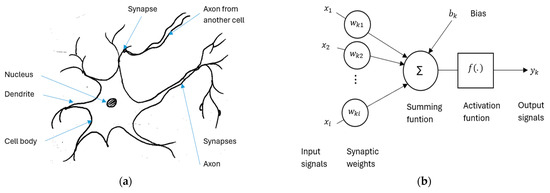
Figure 1.
Neuron’s points of convergence as: (a) Simplified biological neuron model; (b) Artificial neuron [47].

Table 1.
Biological neuron’s and artificial neuron’s points of convergence.
As shown in Figure 2, the ANN consists of three types of nodes, which can be differentiated based on their roles.
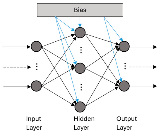
Figure 2.
Artificial neural network [48].
Input nodes receive continuous or discrete signals, which are transferred to the hidden nodes through interconnected weights. The primary distinction between the input and hidden layers is that while the hidden layers process the data, the input nodes merely pass it into the network. Finally, the output nodes generate the network’s final results. In deep learning, artificial neural networks have multiple hidden layers that facilitate mapping complex relationships between input and output nodes [49].
2.2. Artificial Neural Network Architecture
Considering the ANN in Figure 2 for regression or classification tasks, the input vector and their weight vector were used to find the input vector of the activation function at the two nodes of the hidden layer:
After receiving signals from the bias and the two inputs, the nodes in the hidden layer make the sum of all input values before processing it through the activation functions. The outputs of the activation function at each node of the hidden layer can be found as follows:
The output of the activation function at each node of the hidden layer can then be used as inputs of the activation function of the output layer. Therefore, the input and output vector of the activation function at the output layer were, respectively, calculated by analogy to Equations (1) and (2). It means that the output vector of the hidden layer and the weight vector were used to find the input vector of the activation function at the output layer:
The outputs of the activation function at the output layer can be found as follows:
2.2.1. Classical Activation Function
An activation function is a mathematical equation determining whether a neuron should be activated. It introduces nonlinearity, allowing the model to learn complex relationships between the input and output data flows [50].
The sigmoid function generates output as the probability of a Boolean signal based on the input value. When the input is negative, there is a high likelihood that the output will be zero; conversely, when the input is positive, the probability of the output being one increases. This activation function is primarily utilized for classification tasks. The mathematical relationship between the input and output can be defined as follows [51]:
The linear activation function does not perform any transformation on the input data; it essentially means that the input value is directly transmitted to the output, regardless of whether it is negative or positive. The mathematical relationship between the input and output can be expressed as follows:
ReLU (Rectified Linear Unit) is a variation in the linear activation function, which transmits input values to the output only for positive values. For negative values, the output is consistently zero. The mathematical relationship between the input and output can be expressed as:
2.2.2. Fundamentals of Quantum Computing
Quantum computing marks a significant shift from the principles of classical computation. Unlike traditional systems that manipulate information through binary bits restricted to values of 0 or 1, quantum systems employ quantum bits, or qubits, which follow the rules of quantum mechanics. The behavior of qubits is governed by two core quantum phenomena-superposition and entanglement-enabling them to encode not only 0 or 1 but also any linear combination of both states simultaneously [9,52]. Through superposition, a qubit can exist in a blended state of and . Mathematically, its state is described as a linear superposition of the computational basis vectors [53]:
Here, and are complex coefficients denoting probability amplitudes. Upon measurement, the likelihood of observing the qubit in equals , while the probability of collapsing to is given by . These values must satisfy the normalization rule, [52].
A convenient representation of qubit states is offered by the Bloch sphere, where and lie along orthogonal directions. Any qubit state can be expressed using spherical coordinates defined by the angles and [54]:
In this formulation, specifies the polar angle from the north pole of the sphere, while denotes the azimuthal angle. Qubit manipulation is achieved through quantum gates, which are unitary operators analogous to classical logic gates but inherently reversible. Rotations about the Bloch sphere’s axes constitute basic operations, implemented by rotation operators such as [55]:
where , and correspond to rotations around the , and z axes, respectively. Another cornerstone of quantum mechanics is entanglement, a phenomenon in which qubits become inseparably correlated so that the state of one immediately reflects the state of the other, regardless of distance [56]. Entanglement enables the creation of multi-qubit states crucial for quantum algorithms. A key operation in generating such correlations is the rotation, which facilitates the formation of superpositions and entangled states. This process underpins advanced applications such as quantum error correction and teleportation [57,58].
2.2.3. Quantum-Inspired Activation Function
The concept is to define the qubit state as a function of the classical input Z and then employ quantum computing principles, including superposition and quantum measurement. The qubit’s measurement product will deliver the probability that it performs as the output of our quantum activation function [52,56,57]. Thus, the qubit state is a function of the input Z. Considering a qubit state , the input of the quantum activation function is defined as a function of Z [58]. The qubit state can then be expressed as:
The parameter , constrained within the interval , characterizes the probability amplitudes associated with the computational basis states and . In contrast, the parameter , defined over the range , determines the relative phase between these two basis components. Together, and fully specify the state of a single qubit on the Bloch sphere [57,58,59].
To express the qubit as a function of the input Z, we took equal to 0 rad and the angle was taken as the product of and the output of the classical sigmoid function of Z. These operations map values between zero and rad.
After performing quantum measurement of |ψ⟩, if the obtained result gives |0⟩, it means that the probability of |ψ⟩ being in the classical state |0⟩ is more than the probability of |ψ⟩ being in the classical state :
Quantum measurement of |ψ⟩ gives , when the probability of being in the classical state is less or equal to the probability of |ψ⟩ being in the classical state :
Specifically, the probability of the quantum state collapsing to the classical basis state upon measurement is given by , while the probability of it collapsing to the basis state is given by . These probabilities arise from the squared magnitudes of the corresponding probability amplitudes in the state vector representation [56,59].
Quantum-inspired sigmoid activation function takes as input and then performs a quantum measurement on it; the output is the value of the probability of being in the classical state :
Figure 3 provides graphs of the classical and quantum sigmoid functions to compare their convergence and divergence.
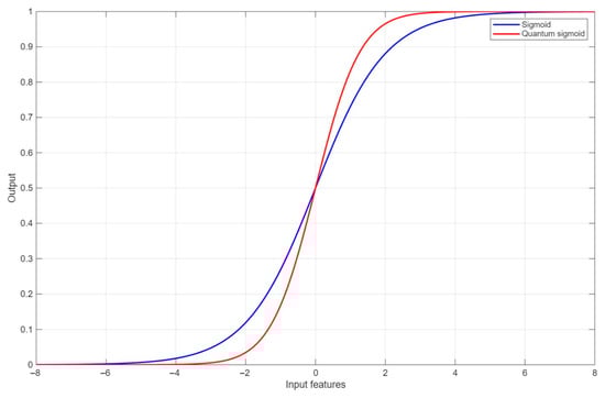
Figure 3.
Comparison of classical sigmoid and quantum sigmoid functions.
The two sigmoid functions are quite similar in their behavior; they start from minus infinity with both outputs set at zero before increasing gradually, respectively, at input values of −6 for classical sigmoid and −4 for quantum sigmoid. The two sigmoids converge at an input of 0, where they yield outputs equal to 0.5; Beyond this point, the output of the quantum sigmoid function surpasses the output value of classical sigmoid for the same input value. Quantum-inspired sigmoid reaches its maximum output for inputs superior or equal to 4, whereas classical sigmoid reaches its maximum output for inputs superior or equal to 6.
Quantum-inspired Relu activation function was taken as the quantum-inspired sigmoid function weighted by the initial classical value of Z:
To compare graphs of the classical and the quantum Relu activation functions, Figure 4 was provided below:
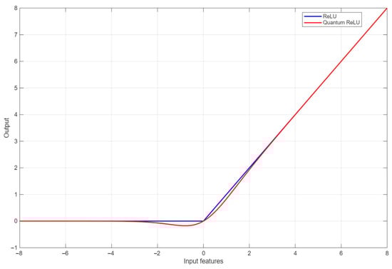
Figure 4.
Comparison between classical and quantum-inspired Relu activation functions.
The two Relu activation functions have a lot of similarity in their behaviors; for negative values they both give as output 0, while for positive input values, they give the identical values as output. However, between −2 and 2 as input values, the quantum-inspired Relu activation function gives back identical values with a small transformation. In other words, the output values were a little bit smaller than the expected output values.
Quantum-inspired linear activation function takes as input and then performs a quantum measurement on it. If the classical input Z is negative, the value of the probability of being in the classical state weighted by the initial classical value Z will be considered as the output. Consequently, if the classical input Z was positive, the value of the probability of being in the classical state weighted by the initial classical value Z will be considered as the output:
To compare graphs of the classical and quantum linear activation functions, Figure 5 was provided below:
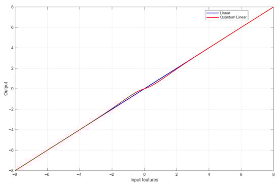
Figure 5.
Comparison between classical and quantum-inspired linear activation functions.
As for the linear activation functions, classical and quantum-inspired linear activation functions are quite similar; they give back as output the identical values regardless of the positive and negative signs of the input values. However, between −2 and 0 as input values, the quantum-inspired function’s output experienced a small transformation where the values were a little bit bigger than the expected values. And between 0 and 2 as input values, the quantum-inspired function’s output experienced a small transformation where the values became a little bit smaller than the expected values.
2.2.4. Development of a QANN Architecture for the Regression Task
The ANN inspired by quantum computing was implemented and trained to estimate mass and moment of inertia of Car-Like Mobile Robot using its RMSE between the desired and the robot’s actual trajectory. The training of this QANN was carried out using a considerable amount of data Where masses values were between 5 and 20 kg, while moments of inertia values between 0.1 and 0.25 .
To confine the parameters of the QANN architecture, we examined mobile robots tasked with tracking a combination of linear and curvy trajectory. The dynamic constraints and the absence of an optimization process made it impossible for the robots to adhere to the desired path perfectly. By examining the RMSEs of the robots at 20 identical points within the simulation, denoting the number of inputs for the QANN, and allocating a value of two to the outputs, which correspond to the robots’ masses and moments of inertia, we can establish the mathematical relationship between the inputs and outputs.
For weight and bias optimization, the input vector X and the weight vector are considered. This allows us to find the input vector for the activation functions at the 20 nodes of the hidden layer.
To find the input vector of the activation functions at the 20 nodes of the hidden layer in the quantum form according to Equations (13) and (14):
The output vector of the quantum-inspired activation functions at each node of the hidden layer can be found as follows:
The output vector of quantum-inspired activation functions at each node of the hidden layer and its vector of weights were used to find the input vector of the activation functions at the output layer:
To find the input vector of the activation functions at the 2 nodes of the output layer in their quantum form, the analogy to relations (13) and (14) was considered:
The outputs of the activation function at the output layer in their quantum forms can be found analogically to Equation (19):
Backward propagation was implemented to correct the cost function, which is the root mean squared error between the predicted output of the CANN/QANN and the true value of the training set. The idea is to minimize the cost function using an optimization algorithm; knowing that the more the cost function tends toward zero, the more precise the model is to predict the output values knowing the input values. The first derivate of the vector of weights, which are located between the hidden layer and the output layer:
Here, der (·) denotes the partial derivative of the cost function with respect to the indicated parameter. In this expression, is the vector of predicted outputs from the quantum-inspired linear activation function, is the vector of true target values (mass and moment of inertia), and denotes the quantum-inspired ReLU outputs from the hidden layer; their outer product yields the gradient of the weights between the hidden and output layers. Update of the vector of weights, which are located between the hidden and the output layers each iteration:
This equation updates the hidden-to-output weight matrix by subtracting the product of the learning rate and its corresponding gradient, steering the weights in the direction that reduces prediction error. The first derivate of the vector of bias, which is located between the hidden and the output layers:
The bias gradient at the output layer is calculated as the difference between the predicted output and the true output, representing the output-layer error. Update of the vector of bias, which is located between the hidden and the output layers, matrix:
Here, the output-layer bias vector , a matrix, is updated by subtracting its gradient scaled by the learning rate. The first derivate of the vector of the activation functions, which are located between the input and the hidden layers, matrix:
This term represents the backpropagated error at the hidden layer, computed by multiplying the transposed output-layer weight matrix with the output error, and serves as the sensitivity vector for the hidden layer. The first derivate of the input vector of the activation functions, which are located at the 20 nodes of the hidden layer:
The expression refers to the derivative of the quantum-inspired ReLU activation function with respect to the pre-activation input ; these derivatives capture how small changes in the hidden-layer inputs affect the nonlinear quantum activation outputs during backpropagation. In this step, the derivative of the hidden-layer pre-activation values is computed by multiplying the local error signal from each neuron with the derivative of the corresponding quantum-inspired ReLU activation function. The first derivate of the vector of the weights, located between the input and the hidden layers:
The gradient of the input-to-hidden weight matrix is obtained by multiplying the vector of hidden-layer pre-activation gradients with the transpose of the input vector . Here, denotes the 20-dimensional input vector composed of RMSE values calculated at discrete points along the robot’s trajectory, each representing the deviation between the desired and actual positions at that point in time. Update of the vector of the weights, located between the input and the hidden layers:
This equation updates the weight matrix by subtracting the scaled gradient from its current value, facilitating the adjustment of how input features influence the hidden neurons. The first derivate of the vector of the bias, which is located between the input and the hidden layers:
The gradient of the hidden-layer bias vector is equal to the derivative of the hidden pre-activation vector , reflecting how much each bias term contributes to the error. Update of the vector of the bias, which is located between the input layer and the hidden layer:
Lastly, the hidden-layer biases are updated by subtracting the gradient scaled by the learning rate from the current bias vector, ensuring that each neuron’s bias is refined during training to reduce output error.
Both the CANN and QANN were developed with highly similar overall architectures to ensure a reasonable comparison. Each model processes a 20-dimensional input vector of RMSE values, passes it through a hidden layer of 20 neurons, and outputs two values corresponding to the robot’s mass and moment of inertia. Both architectures were trained for 5000 epochs using a PSO-optimized learning rate, 50 particles, scaled velocity factor 0.5, 100 iterations, with RMSE serving as the cost function. The datasets for training 50 configurations and validation 21 configurations were purposely left unnormalized to replicate raw real-world conditions. The main architectural difference lies in the activation functions. While CANN employs traditional nonlinear functions, QANN integrates hybrid quantum-inspired activation functions that combine quantum principles to simulate qubit dynamics, thereby enhancing the network’s representational power.
To additionally describe this distinction, it is important to note that the CANN employs standard sigmoid, ReLU, and linear activations. In contrast, the QANN replaces them with hybrid counterparts that map the classical input z to a qubit state and use measurement probabilities as outputs. This probabilistic weighting maintains the overall shape of the classical functions while introducing adaptive rescaling around critical regions, such as near zero or in early saturation, so heightening nonlinearity and representation without altering the overall architecture. Table 2 provides a summary of the differences in activation functions between the implementations in CANN and QANN for each function.
Table 2.
Comparison between classical and quantum-inspired activation functions.
2.3. Mobile Robot Model
Deriving the equations of motion is required for the effective modeling, control, and path planning of car-like mobile robots (CLMR). These equations form the foundation for creating accurate controllers and navigation strategies that improve path-tracking performance. In this study, we employ the Euler–Lagrange formalism, leveraging the nonlinear dynamic characteristics of the system as depicted in Figure 6, which enables the explicit incorporation of inertial, Coriolis, and gravitational effects [51,60]. Such a formulation enhances the accuracy of the dynamic model and provides a systematic framework for designing energy-efficient and robust control strategies suitable for real-time implementation.
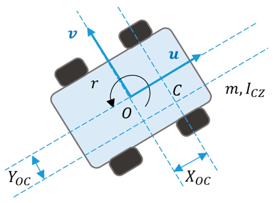
Figure 6.
The mobile robot dynamics within a 2D planar surface.
Both linear velocity components at the robot’s center of mass, projected along the x-axis and y-axis, are mathematically defined as:
Here, and represent the distances from the origin of the body frame to the center of mass along the x- and y-directions, respectively, while and denote the corresponding velocities at the center of mass. The translational velocities and , together with the angular velocity , capture the complete kinematic state of the mobile robot in body-fixed coordinates.
The robot’s equations of motion, defined with respect to its body-fixed frame, are formulated as follows:
In these expressions, is the robot’s total mass, is the moment of inertia about the z-axis, and is the robot’s angular velocity. For the configuration considered in this study, the center of mass coincides with the origin of the body frame, implying that both and are equal to zero. This simplifies the dynamic equations, allowing the torque applied to the car-like mobile robot to be directly influenced by its linear and angular accelerations. Accordingly, the system dynamics can be represented compactly in matrix form:
So that, is the vector of generalized accelerations representing the CLMR’s nonholonomic motion behavior, is the total torque vector acting on the system; is the dynamic (inertia) matrix capturing the system’s mass distribution and resistance to acceleration; and aggregates Coriolis and centrifugal effects. Having an accurate estimate of the robot’s position, applied forces, and inertial characteristics enable real-time adjustment of velocity and acceleration commands. This dynamic recalibration ensures that torque and control signals are precisely tuned, resulting in enhanced path following performance for the CLMR.
3. Results and Discussion
3.1. Simulation Parameters
Both models were developed using a standardized architecture and dataset to assess and compare the performance of Classical Artificial Neural Networks and Quantum-Inspired Artificial Neural Networks in estimating the mass and moment of inertia of a car-like mobile robot. This comparative framework ensures that any differences observed in predictive accuracy or convergence behavior can be directly attributed to the model architecture itself, rather than variations in training conditions. Table 3 provides a summary of key architectural parameters, including the number of layers, activation functions, and learning rates, as well as the simulation settings employed to maintain consistency across all experiments.
Table 3.
Neural Network Architecture and Training Parameters.
The dataset used in this study was derived from a previous trajectory-tracking experiment involving a car-like mobile robot [60]. In that work, we employed a Quantum Particle Swarm Optimization (QPSO) algorithm to refine the robot’s trajectory based on a dynamic model that included mass, moment of inertia, viscous coefficients, and a fixed desired trajectory. For the current analysis, we simulated multiple robot configurations by systematically varying the mass and moment of inertia. Each configuration attempted to follow the same desired path without optimization, leading to deviations caused by dynamic constraints. These deviations were quantified as RMSE values by comparing the actual and desired trajectories. As a result, the dataset includes triplets of mass, moment of inertia, and their associated RMSE profiles, which can serve as a valuable resource for future research in robot trajectory tracking and optimization algorithms. The formal definition of these deviations and the computation of the RMSE values are presented in the following formulation and in standard PD control for trajectory tracking, the position error is defined as follows [60]:
where denotes the desired trajectory of the robot at time step , and represents the actual trajectory measured at the same instant. To quantify the deviation between the desired and actual trajectories, the Root Mean Square Error (RMSE) was calculated as:
where is the total number of discrete sampling points along the trajectory, is the -th time step, and is the position error at that time step. This formulation ensures that the RMSE provides a single scalar value representing the overall tracking performance for each robot configuration. These RMSE values were then used to construct the dataset, where each entry consists of the mass, moment of inertia, and the corresponding RMSE profile. In this study, no control law is implemented or analyzed. The PD–QPSO controller referenced from [60] is only used as the source of the trajectory data, from which RMSE profiles were computed for training the neural models.
Each model takes a 20-dimensional input vector representing the RMSE values calculated at 20 discrete points along the robot’s trajectory. These values characterize the differences between the desired and actual trajectories, providing indirect insights into the robot’s underlying dynamics. The output layer consists of two neurons corresponding to the predicted mass and moment of inertia.
The number of hidden layer nodes was empirically chosen to be 20 based on preliminary investigations that pointed out that this size strikes a promising balance between model expressiveness and the risk of overfitting. A fixed training epoch of 5000 iterations was set to allow sufficient convergence for both architectures while facilitating comparative analysis of their training dynamics. The selection of 20 input nodes was designed to capture essential details throughout the robot’s trajectory. With adequately distinct robot configurations simulated, each exhibiting varying mass and moment of inertia values, unique actual trajectories were generated while adhering to the exact desired path. The 20 chosen time points provided a representative sampling of critical trajectory deviations, allowing the network to learn the dynamic relationships effectively. Additionally, 20 hidden nodes were selected to maintain architectural symmetry, a design principle that ensures the network’s structure is balanced and organized, and to ensure sufficient learning capacity without the risk of overfitting.
The learning rates for both the CANN and QANN were deliberately optimized rather than chosen at random. This optimization was achieved through Particle Swarm Optimization (PSO), a bio-inspired, population-based metaheuristic algorithm designed to minimize the training cost function. By employing this method, we ensured that both neural networks operated under near-optimal learning conditions specifically tailored to their unique architectures. The search space for learning rates was defined within the interval [0, 1] to facilitate this. A swarm of 50 particles was initialized with random positions and velocities, the latter scaled by a factor of 0.5 to prevent overshooting. Each particle represented a potential learning rate and was assessed using the RMSE-based cost function. Throughout 100 iterations, the swarm evolved as particles adjusted their positions using both personal best and global best information. The learning rate that minimized the cost function across all particles and iterations was ultimately chosen for model training.
The training dataset comprised 1000 unique data points, each representing a dis-tinct robot configuration and its corresponding RMSE profile. An independent validation dataset containing 100 entries was utilized to evaluate generalization performance. This validation dataset was purposefully left unnormalized to duplicate real-world scenarios where incoming data may vary in scale, variance, or feature distribution. Notably, no normalization was applied to either the input or output data in this study. This design decision was made to evaluate the models’ true generalization capabilities in conditions that resemble raw real-world data without artificial preprocessing to equalize feature scales. This design choice facilitates a robust evaluation of the models’ generalization abilities under non-ideal input conditions, essential for practical implementation in a real-time setting.
3.2. Training Process Results
To estimate the proposed neural network models’ learning performance and convergence dynamics, both CANN and QANN were trained over 5000 iterations using the same dataset. The performance was assessed using the Root Mean Square Error between the predicted and actual values of the robot’s mass and moment of inertia. This cost function directly measures the model’s predictive accuracy regarding the mobile robot’s physical parameters. Figure 7 illustrates the evolution of the cost functions for the CANN and QANN models over multiple iterations. These cost functions were determined by calculating the root mean square errors between the predicted and actual values of the robot’s masses and moments of inertia.
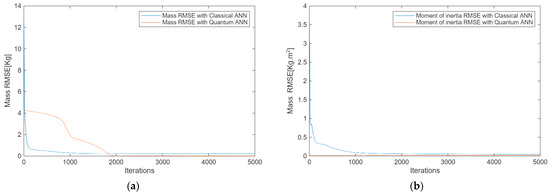
Figure 7.
The evolution over iterations of the cost functions for: (a) Masses evolution; (b) Moments of inertia.
Figure 7a illustrates the performance of CANN and QANN in minimizing their cost functions, which resulted in accurate mass predictions. Both artificial neural networks (ANNs) exhibited similar trends, with average errors decreasing from 4.3 kg for QANN and 11.7 kg for CANN. By the 2000th iteration, the cost functions dropped significantly to 0.031 kg for QANN and 0.041 kg for CANN. As iterations progressed, the average errors continued to decline, albeit at a slower pace, ultimately reaching 0.0028 kg for QANN and 0.0031 kg for CANN by the 5000th iteration.
Figure 7b presents the performances of CANN and QANN in reducing their cost functions for predicting the moment of inertia. Again, both ANNs demonstrated comparable behavior, with initial average errors of 0.03 for QANN and 3.8 for CANN. By the 1000th iteration, these errors decreased to 0.025 for QANN and 0.71 for CANN. Figure 7b shows that the cost functions gradually decreased with each iteration, eventually reaching 0.0132 for QANN and 0.1789 for CANN at the 5000th iteration. Both ANNs were trained over 100 iterations, and consistently, QANN outperformed CANN in effectively reducing cost functions for both mass and moment of inertia estimates. This consistent performance suggests a promising future for QANN in various applications. While CANN managed to lower cost functions to acceptable levels, it tended to become trapped in local minima and overfit the data.
An alternative approach to demonstrating the superiority of QANN over CANN is by comparing the accuracy of predictions against the actual data from the training set, as illustrated in Figure 8 and Figure 9.
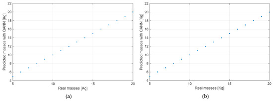
Figure 8.
Comparison between real mass data and those predicted by: (a) QANN; (b) CANN.
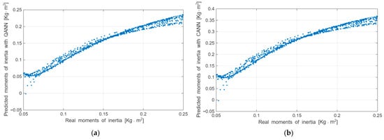
Figure 9.
Comparison between actual moment of inertia data and those predicted by: (a) QANN; (b) CANN.
Figure 8a showcases the precision of QANN’s predictions. For each real mass value on the x-axis, QANN consistently predicts corresponding values within a narrow margin of 0.0028 kg on the y-axis. In contrast, Figure 8b demonstrates that CANN’s predictions deviate more, with a mean error of 0.0031 kg on the y-axis. While CANN’s accuracy is a bit lower than QANN’s precision; both model’s predictions are quite similar
Figure 9 indicates that both types of artificial neural networks predict different moments of inertia with acceptable accuracy: QANN achieves an accuracy of 0.0132 , while CANN reaches 0.1789 . In all instances, QANN demonstrates superior performance in predicting moments of inertia.
The results from the training process clearly show that QANN is more effective in reducing the cost function. This is a significant finding, as it signifies that QANN outperforms CANN in predicting the masses and moments of inertia of the robot. The predictions made by QANN are much closer to the actual values in the training database, demonstrating its effectiveness. Table 4 summarizes the training outcomes for CANN and QANN to consolidate the comparative performance of both neural network models. The table includes RMSE values at critical stages of the training process for predicting both mass and moment of inertia. Additionally, it highlights each model’s prediction accuracy, generalization behavior, and consistency across repeated trials.
Table 4.
Summary of Training Outcomes for CANN compared with QANN.
In summary, the training results highlight the different advantages of the quantum-inspired neural network compared to its classical counterpart. The QANN exhibited faster convergence, enhanced prediction accuracy, and improved stability throughout all training trials. It consistently achieved more precise estimations of both mass and moment of inertia while demonstrating robustness throughout the learning process. In contrast, the CANN exhibited tendencies toward overfitting and was sensitive to local minima. However, the QANN’s unique ability to capture involved, nonlinear relationships in robotic dynamics were a key advantage, as it maintained reliable performance as training advanced. These findings highlight the possibility of quantum-inspired architectures for broader applications in real-time estimation and control tasks.
3.3. Results’ Validation
Predictions from both models were compared using an independent validation dataset to estimate and validate the generalization capabilities of the Quantum-Inspired Artificial Neural Network and the Classical Artificial Neural Network. This measure is essential for confirming the robustness of the models and their ability to sustain predictive accuracy when applied to previously overlooked data, thereby simulating requirements closer to real-world deployment scenarios. Figure 10 delivers a straightforward comparison between the actual values and the predictions generated by both neural networks for mass and moment of inertia parameters.
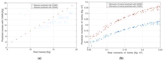
Figure 10.
Comparison between actual and predicted data for: (a) Masses; (b) Moments of Inertia.
In Figure 10a, the predictions for mass show reasonable accuracy from both QANN and CANN, closely aligning with the diagonal line that represents perfect prediction accuracy. Both models achieved identical root mean square errors about RMSE of approximately 0.003 kg, offering substantial generalization capabilities and consistent performance when faced with unseen data. The predictions closely reach the ideal values across the entire tested mass range among 5–20 kg, accentuating the effectiveness of both QANN and CANN in accurately evaluating mass in practical applications.
Figure 10b depicts a clear difference between QANN and CANN in their predictions of moments of inertia. QANN’s predictions invariably align with the actual values, achieving a validation RMSE of 0.0195 , which indicates firm agreement and stability compared to its training dataset performance in RMSE of 0.0132 . Nevertheless, CANN’s predictions show a much wider distribution and more influential deviation, particularly at higher inertia values. The validation dataset’s RMSE for CANN increased significantly to 0.125 , demonstrating a noteworthy decline in predictive reliability relative to its training performance, which emphasizes the demand for further research and progress in CANN’s predictive capabilities.
The discrepancy between the performance of QANN and CANN highlights an important distinction, QANN exhibits a stable predictive capability, effectively balancing the complexity of learned relationships with the ability to generalize across new data points. In contrast, the CANN shows signs of overfitting, performing well during training validation, particularly with complicated predictions involving higher moments of inertia.
In conclusion, the validation results reaffirm QANN’s benefits, particularly its superior capacity to generalize without succumbing to common modeling challenges such as overfitting or underfitting. The consistent predictive accuracy of QANN across both mass and moment of inertia, even for previously unseen data, verifies its robustness and reliability for real-world robotics applications.
4. Conclusions
The comparative evaluation of two distinct neural architectures, a Classical Artificial Neural Network and a Quantum-Inspired Artificial Neural Network, demonstrated clear advantages in integrating quantum-inspired computation for dynamic parameter estimation in mobile robotics. Leveled in classic learning theory, CANN served as a performance baseline. At the same time, QANN, designed using principles such as quantum superposition and probabilistic measurement, exhibited better predictive accuracy, convergence behavior, and generalization capacity. Over 100 simulation independent trials, QANN consistently outperformed CANN, achieving a 9.7% reduction in training RMSE for mass from 0.0031 kg to 0.0028 kg and an 84.4% decrease in validation RMSE for moment of inertia from 0.125 kg·m2 to 0.0195 kg·m2. Additionally, QANN displayed better generalization and robustness in regression and classification tasks.
These findings highlight the advantages of integrating quantum computing principles into classical machine learning frameworks. Quantum-inspired artificial Neural networks’ enhanced convergence, stability to overfitting, and stable prediction results signify a profitable advancement for high-precision dynamic parameter estimation in robotic control systems. More importantly, they instill confidence in its robust performance, particularly in situations that demand accurate real-time modeling, reassuring the audience about its performance in challenging situations.
However, this study’s limitation is that it focuses only on simulated data, based on a relatively modest dataset. The models have yet to be tested in real-world conditions, where factors such as sensor noise, nonlinear dynamics, and system uncertainties could impact performance. Therefore, future research should focus both on validating these findings under real-world conditions and on expanding the dataset to ensure more comprehensive and reliable evaluation of the proposed QANN framework.
Future research to enhance the quantum model of the network involves implementing the QANN architecture on different embedded robotic platforms and evaluating its performance under varying environmental conditions. This step holds significant promise for the future of robotic applications, as QANN’s potential in real-world scenarios, including multi-joint manipulators, unmanned aerial vehicles (UAVs), and cooperative multi-agent platforms, is yet to be thoroughly investigated. Additionally, focus on expanding the dataset, as the current architecture requires a larger volume of data to effectively optimize its numerous trainable parameters and more reliably minimize the cost function. Beyond dataset expansion, future studies will also incorporate randomized training and validation splits, such as cross-validation, to provide a more statistically rigorous assessment of model performance and to confirm the robustness of the QANN framework across multiple data partitions. These future directions will provide broader validation of the QANN framework, offering further confirmation of its robustness, adaptability, and general applicability across diverse robotic domains. Moreover, future research may also extend toward closed-loop stability analysis for car-like robots under nonholonomic constraints and viscous environments, which lies beyond the current parameter-estimation scope.
In conclusion, the current research underscores the influential potential of quantum-inspired neural models. The advantageous performance of QANN in this study particularly enhances our anticipation for its future applications, where it can seriously enhance precision, adaptability, and computational efficiency in autonomous robotic systems.
Author Contributions
J.N. contributed to methodology, investigation, formal analysis, writing editing of the original draft, and visualization. M.F. contributed to methodology, formal analysis, writing editing of the original draft, and visualization. N.Z. contributed to providing resources, supervision, project administration, formal analysis, review and editing of the original draft, funding acquisition, and visualization. All authors have read and agreed to the published version of the manuscript.
Funding
This work was financially supported by NSERC Canada.
Data Availability Statement
The data supporting the findings of this study are not publicly available as they are part of ongoing research and future work. Data may be shared upon reasonable request after the completion of future studies.
Conflicts of Interest
The authors declare no conflicts of interest.
Abbreviations
The following abbreviations are used in this manuscript:
| ANN | Artificial Neural Network |
| CANN | Classical Artificial Neural Network |
| CAVs | Connected and Autonomous Vehicles |
| CLMR | Car-Like Mobile Robot |
| DDPG | Deep Deterministic Policy Gradient |
| LiDAR | Light Detection and Ranging |
| LSTM | Long Short-Term Memory |
| MARL | Multi-Agent Reinforcement Learning |
| MSE | Mean Squared Error |
| NISQ | Noisy Intermediate-Scale Quantum |
| PSO | Particle Swarm Optimization |
| QANN | Quantum-Inspired Artificial Neural Network |
| Q-DDPG | Quantum Deep Deterministic Policy Gradient |
| Q-RDDPG | Quantum Recurrent Deep Deterministic Policy Gradient |
| QRL | Quantum Reinforcement Learning |
| R-CNN | Region-based Convolutional Neural Network |
| R-FCN | Region-based Fully Convolutional Network |
| ReLU | Rectified Linear Unit |
| RGB | Red Green Blue (color space used in imaging) |
| RMSE | Root Mean Squared Error |
| USV | Unmanned Surface Vehicle |
| LR | Learning Rate |
| q-FPS | Quantum Fast Path Search |
| q-RRT | Quantum Rapidly Exploring Random Tree |
| UAV | Unmanned Aerial Vehicles |
References
- Alexa, O.; Ciobotaru, T.; Grigore, L.Ș.; Grigorie, T.L.; Ștefan, A.; Oncioiu, I.; Priescu, I.; Vlădescu, C. A Review of Mathematical Models Used to Estimate Wheeled and Tracked Unmanned Ground Vehicle Kinematics and Dynamics. Mathematics 2023, 11, 3735. [Google Scholar] [CrossRef]
- Leboutet, Q.; Roux, J.; Janot, A.; Guadarrama-Olvera, J.R.; Cheng, G. Inertial parameter identification in robotics: A survey. Appl. Sci. 2021, 11, 4303. [Google Scholar] [CrossRef]
- Siwek, M.; Panasiuk, J.; Baranowski, L.; Kaczmarek, W.; Prusaczyk, P.; Borys, S. Identification of differential drive robot dynamic model parameters. Materials 2023, 16, 683. [Google Scholar] [CrossRef]
- Wu, J.; Wang, J.; You, Z. An overview of dynamic parameter identification of robots. Robot. Comput. Manuf. 2010, 26, 414–419. [Google Scholar] [CrossRef]
- Mavrakis, N.; Stolkin, R. Estimation and exploitation of objects ’ inertial parameters in robotic grasping and manipulation: A survey. Robot. Auton. Syst. 2020, 124, 103374. [Google Scholar] [CrossRef]
- Zhu, M.; Gong, D.; Zhao, Y.; Chen, J.; Qi, J.; Song, S. Compliant Force Control for Robots: A Survey. Mathematics 2025, 13, 2204. [Google Scholar] [CrossRef]
- Lee, T.; Kwon, J.; Wensing, P.M.; Park, F.C. Robot model identification and learning: A modern perspective. Annu. Rev. Control. Robot. Auton. Syst. 2023, 7, 311–334. [Google Scholar] [CrossRef]
- Nguyen-Tuong, D.; Peters, J. Model learning for robot control: A survey. Cogn. Process. 2011, 12, 319–340. [Google Scholar] [CrossRef] [PubMed]
- Fazilat, M.; Zioui, N. Quantum Neural Network-based Inverse Kinematics of a Six-jointed Industrial Robotic Arm. Robot. Auton. Syst. 2025, 194, 105123. [Google Scholar] [CrossRef]
- Wang, Y.; Shen, B.; Nan, Z.; Tao, W. An End-to-End Path Planner Combining Potential Field Method with Deep Reinforcement Learning. IEEE Sensors J. 2024, 24, 26584–26591. [Google Scholar] [CrossRef]
- Mutti, S.; Pedrocchi, N.; Valente, A.; Dimauro, G. Sim-to-Real RNN-Based Framework for the Precise Positioning of Autonomous Mobile Robots. IEEE Access 2024, 12, 163948–163957. [Google Scholar] [CrossRef]
- Ding, L.; Li, S.; Gao, H.; Chen, C.; Deng, Z. Adaptive partial reinforcement learning neural network-based tracking control for wheeled mobile robotic systems. IEEE Trans. Syst. Man, Cybern. Syst. 2018, 50, 2512–2523. [Google Scholar] [CrossRef]
- Saleem, H.; Malekian, R.; Munir, H. Neural network-based recent research developments in SLAM for autonomous ground vehicles: A review. IEEE Sensors J. 2023, 23, 13829–13858. [Google Scholar] [CrossRef]
- Hu, J.; Niu, H.; Carrasco, J.; Lennox, B.; Arvin, F. Voronoi-based multi-robot autonomous exploration in unknown environments via deep reinforcement learning. IEEE Trans. Veh. Technol. 2020, 69, 14413–14423. [Google Scholar] [CrossRef]
- Chen, L.; Lin, S.; Lu, X.; Cao, D.; Wu, H.; Guo, C.; Liu, C.; Wang, F.-Y. Deep neural network based vehicle and pedestrian detection for autonomous driving: A survey. IEEE Trans. Intell. Transp. Syst. 2021, 22, 3234–3246. [Google Scholar] [CrossRef]
- Li, Y.; Wang, H.; Dang, L.M.; Nguyen, T.N.; Han, D.; Lee, A.; Jang, I.; Moon, H. A deep learning-based hybrid framework for object detection and recognition in autonomous driving. IEEE Access 2020, 8, 194228–194239. [Google Scholar] [CrossRef]
- Ravindran, R.; Santora, M.J.; Jamali, M.M. Multi-object detection and tracking, based on DNN, for autonomous vehicles: A review. IEEE Sens. J. 2021, 21, 5668–5677. [Google Scholar] [CrossRef]
- Huang, Z.; Lv, C.; Xing, Y.; Wu, J. Multi-modal sensor fusion-based deep neural network for end-to-end autonomous driving with scene understanding. IEEE Sensors J. 2020, 21, 11781–11790. [Google Scholar] [CrossRef]
- Da Lio, M.; Donà, R.; Papini, G.P.R.; Biral, F.; Svensson, H. A mental simulation approach for learning neural-network predictive control (in self-driving cars). IEEE Access 2020, 8, 192041–192064. [Google Scholar] [CrossRef]
- Steshenko, J.; Kagan, E.; Ben-Gal, I. A simple protocol for a society of NXT robots communicating via Bluetooth. In Proceedings of the ELMAR-2011, Zadar, Croatia, 14–16 September 2011. [Google Scholar]
- Mahanti, S.; Das, S.; Behera, B.K.; Panigrahi, P.K. Quantum robots can fly; play games: An IBM quantum experience. Quantum Inf. Process. 2019, 18, 219. [Google Scholar] [CrossRef]
- Atchade-Adelomou, P.; Alonso-Linaje, G.; Albo-Canals, J.; Casado-Fauli, D. qRobot: A quantum computing approach in mobile robot order picking and batching problem solver optimization. Algorithms 2021, 14, 194. [Google Scholar] [CrossRef]
- Sarkar, M.; Pradhan, J.; Singh, A.K.; Nenavath, H. A novel hybrid quantum architecture for path planning in quantum-enabled autonomous mobile robots. IEEE Trans. Consum. Electron. 2024, 70, 5597–5606. [Google Scholar] [CrossRef]
- Bogue, R. Quantum technologies in robotics: A preliminary appraisal. Ind. Robot. Int. J. Robot. Res. Appl. 2025, 52, 1–8. [Google Scholar] [CrossRef]
- Panda, B.; Tripathy, N.K.; Sahu, S.; Behera, B.K.; Elhady, W.E. Controlling Remote Robots Based on Zidan’s Quantum Computing Model. Comput. Mater. Contin. 2022, 73, 6225–6236. [Google Scholar] [CrossRef]
- Petschnigg, C.; Brandstotter, M.; Pichler, H.; Hofbaur, M.; Dieber, B. Quantum computation in robotic science and applications. In Proceedings of the 2019 International Conference on Robotics and Automation (ICRA), Montreal, Canada, 20–24 May 2019. [Google Scholar]
- Yan, F.; Iliyasu, A.M.; Li, N.; Salama, A.S.; Hirota, K. Quantum robotics: A review of emerging trends. Quantum Mach. Intell. 2024, 6, 86. [Google Scholar] [CrossRef]
- Peixoto, M.L.M. Quantum Edge Computing for Data Analysis in Connected Autonomous Vehicles. In Proceedings of the 2024 IEEE Symposium on Computers and Communications (ISCC), Paris, France, 26–29 June 2024. [Google Scholar]
- Chella, A.; Gaglio, S.; Mannone, M.; Pilato, G.; Seidita, V.; Vella, F.; Zammuto, S. Quantum planning for swarm robotics. Robot. Auton. Syst. 2023, 161, 104362. [Google Scholar] [CrossRef]
- Mannone, M.; Seidita, V.; Chella, A. Modeling and designing a robotic swarm: A quantum computing approach. Swarm Evol. Comput. 2023, 79, 101297. [Google Scholar] [CrossRef]
- Gehlot, V.P.; Balas, M.J.; Quadrelli, M.B.; Bandyopadhyay, S.; Bayard, D.S.; Rahmani, A. A Path to Solving Robotic Differential Equations Using Quantum Computing. J. Auton. Veh. Syst. 2022, 2, 031004. [Google Scholar] [CrossRef]
- Lathrop, P.; Boardman, B.; Martínez, S. Quantum search approaches to sampling-based motion planning. IEEE Access 2023, 11, 89506–89519. [Google Scholar] [CrossRef]
- Xia, G.; Han, Z.; Zhao, B.; Wang, X. Local path planning for unmanned surface vehicle collision avoidance based on modified quantum particle swarm optimization. Complexity 2020, 2020, 3095426. [Google Scholar] [CrossRef]
- Chalumuri, A.; Kune, R.; Kannan, S.; Manoj, B.S. Quantum–classical image processing for scene classification. IEEE Sensors Lett. 2022, 6, 1–4. [Google Scholar] [CrossRef]
- Islam, M.; Chowdhury, M.; Khan, Z.; Khan, S.M. Hybrid quantum-classical neural network for cloud-supported in-vehicle cyberattack detection. IEEE Sensors Lett. 2022, 6, 1–4. [Google Scholar] [CrossRef]
- Salek, M.S.; Biswas, P.K.; Pollard, J.; Hales, J.; Shen, Z.; Dixit, V.; Chowdhury, M.; Khan, S.M.; Wang, Y. A novel hybrid quantum-classical framework for an in-vehicle controller area network intrusion detection. IEEE Access 2023, 11, 96081–96092. [Google Scholar] [CrossRef]
- Hohenfeld, H.; Heimann, D.; Wiebe, F.; Kirchner, F. Quantum deep reinforcement learning for robot navigation tasks. IEEE Access 2024, 12, 87217–87236. [Google Scholar] [CrossRef]
- Bar, N.F.; Yetis, H.; Karakose, M. An approach based on quantum reinforcement learning for navigation problems. In Proceedings of the 2022 International Conference on Data Analytics for Business and Industry (ICDABI), Virtual Conference, 25–26 October 2022. [Google Scholar]
- Alomari, A.; Kumar, S.A. ReLAQA: Reinforcement Learning-Based Autonomous Quantum Agent for Quantum Applications. IEEE Trans. Artif. Intell. 2024, 6, 549–558. [Google Scholar] [CrossRef]
- Yun, W.J.; Kim, J.P.; Jung, S.; Kim, J. Quantum multiagent actor–critic neural networks for Internet-connected multirobot coordination in smart factory management. IEEE Internet Things J. 2023, 10, 9942–9952. [Google Scholar] [CrossRef]
- Hu, L.; Wei, C.; Yin, L. Fuzzy A∗ quantum multi-stage Q-learning artificial potential field for path planning of mobile robots. Eng. Appl. Artif. Intell. 2025, 141, 109866. [Google Scholar] [CrossRef]
- Li, Y.; Aghvami, A.H.; Dong, D. Intelligent trajectory planning in UAV-mounted wireless networks: A quantum-inspired reinforcement learning perspective. IEEE Wirel. Commun. Lett. 2021, 10, 1994–1998. [Google Scholar] [CrossRef]
- Silvirianti; Narottama, B.; Shin, S.Y. Layerwise quantum deep reinforcement learning for joint optimization of UAV trajectory and resource allocation. IEEE Internet Things J. 2023, 11, 430–443. [Google Scholar] [CrossRef]
- Li, Y.; Aghvami, A.H.; Dong, D. Path planning for cellular-connected UAV: A DRL solution with quantum-inspired experience replay. IEEE Trans. Wirel. Commun. 2022, 21, 7897–7912. [Google Scholar] [CrossRef]
- Park, C.; Yun, W.J.; Kim, J.P.; Rodrigues, T.K.; Park, S.; Jung, S.; Kim, J. Quantum multiagent actor–critic networks for cooperative mobile access in multi-UAV systems. IEEE Internet Things J. 2023, 10, 20033–20048. [Google Scholar] [CrossRef]
- Silvirianti; Narottama, B.; Shin, S.Y. UAV coverage path planning with quantum-based recurrent deep deterministic policy gradient. IEEE Trans. Veh. Technol. 2023, 73, 7424–7429. [Google Scholar] [CrossRef]
- Mirzoev, A.A.; Gelchinski, B.R.; Rempel, A.A. Neural network prediction of interatomic interaction in multielement substances and high-entropy alloys: A review. In Doklady Physical Chemistry; Springer: Berlin/Heidelberg, Germany, 2022. [Google Scholar]
- Aboukarima, A.M.; Elsoury, H.A.; Menyawi, M. Artificial neural network model for the prediction of the cotton crop leaf area. Int. J. Plant Soil Sci. 2015, 8, 1–13. [Google Scholar] [CrossRef]
- Bertsekas, D.; Gallager, R. Data Networks; Athena Scientific: Nashua, NH, USA, 2021. [Google Scholar]
- Meduri, S. Activation functions in neural networks: A comprehensive overview. Int. J. Res. Comput. Appl. Inf. Technol. (IJRCAIT) 2024, 7, 214–227. [Google Scholar] [CrossRef]
- Fathi, E.; Shoja, B.M. Deep neural networks for natural language processing. In Handbook of Statistics; Elsevier: Amsterdam, The Netherlands, 2018; pp. 229–316. [Google Scholar]
- Fazilat, M.; Zioui, N. Quantum Particle Swarm Optimization (QPSO)-Based Enhanced Dynamic Model Parameters Identification for an Industrial Robotic Arm. Mathematics 2025, 13, 2631. [Google Scholar] [CrossRef]
- Fazilat, M.; Zioui, N. Investigating Quantum Artificial Neural Networks for singularity avoidance in robotic manipulators. In Proceedings of the 2024 12th International Conference on Systems and Control (ICSC), Batna, Algeria, 3–5 November 2024. [Google Scholar]
- Fazilat, M.; Zioui, N.; St-Arnaud, J. A novel quantum model of forward kinematics based on quaternion/Pauli gate equivalence: Application to a six-jointed industrial robotic arm. Results Eng. 2022, 14, 100402. [Google Scholar] [CrossRef]
- Fazilat, M.; Zioui, N. Quantum-Inspired Sliding-Mode Control to Enhance the Precision and Energy Efficiency of an Articulated Industrial Robotic Arm. Robotics 2025, 14, 14. [Google Scholar] [CrossRef]
- Zioui, N.; Mahmoudi, A.; Fazilat, M.; Kone, O.; Dermouche, R.; Tadjine, M. Quantum Space Vector Pulse Width Modulation for Speed Control of Permanent Magnet Synchronous Machines. e-Prime-Adv. Electr. Eng. Electron. Energy 2025, 13, 101074. [Google Scholar] [CrossRef]
- Reda, D.; Talaoubrid, A.; Fazilat, M.; Zioui, N.; Tadjine, M. A quantum direct torque control method for permanent magnet synchronous machines. Comput. Electr. Eng. 2025, 122, 109994. [Google Scholar] [CrossRef]
- Feraoun, H.; Fazilat, M.; Dermouche, R.; Bentouba, S.; Tadjine, M.; Zioui, N. Quantum maximum power point tracking (QMPPT) for optimal solar energy extraction. Syst. Soft Comput. 2024, 6, 200118. [Google Scholar] [CrossRef]
- Numbi, J.; Zioui, N.; Tadjine, M. The Concept of Quantum Teleportation for Remote Control of a Car-like Mobile Robot. Robotics 2025, 14, 25. [Google Scholar] [CrossRef]
- Numbi, J.; Zioui, N.; Tadjine, M. Quantum Particle Swarm Optimisation Proportional–Derivative Control for Trajectory Tracking of a Car-like Mobile Robot. Electronics 2025, 14, 832. [Google Scholar] [CrossRef]
Disclaimer/Publisher’s Note: The statements, opinions and data contained in all publications are solely those of the individual author(s) and contributor(s) and not of MDPI and/or the editor(s). MDPI and/or the editor(s) disclaim responsibility for any injury to people or property resulting from any ideas, methods, instructions or products referred to in the content. |
© 2025 by the authors. Licensee MDPI, Basel, Switzerland. This article is an open access article distributed under the terms and conditions of the Creative Commons Attribution (CC BY) license (https://creativecommons.org/licenses/by/4.0/).