Abstract
Accurately estimating a sequence of latent variables in state observation models remains a challenging problem, particularly when maintaining coherence among consecutive estimates. While forward filtering and smoothing methods provide coherent marginal distributions, they often fail to maintain coherence in marginal MAP estimates. Existing methods efficiently handle discrete-state or Gaussian models. However, general models remain challenging. Recently, a recursive Bayesian decoder has been discussed, which effectively infers coherent state estimates in a wide range of models, including Gaussian and Gaussian mixture models. In this work, we analyze the theoretical properties and implications of this method, drawing connections to classical inference frameworks. The versatile applicability of mixture models and the prevailing advantage of the recursive Bayesian decoding method are demonstrated using the double-slit experiment. Rather than inferring the state of a quantum particle itself, we utilize interference patterns from the slit experiments to decode the movement of a non-stationary particle detector. Our findings indicate that, by appropriate modeling and inference, the fundamental uncertainty associated with quantum objects can be leveraged to decrease the induced uncertainty of states associated with classical objects. We thoroughly discuss the interpretability of the simulation results from multiple perspectives.
Keywords:
Bayesian inference; recursive estimation; decoding; state observation model; dynamic systems; Gaussian mixtures; double-slit experiment; quantum-based inference MSC:
62M20
1. Introduction
State observation models play a crucial role in statistical signal processing and inference, where latent variables need to be inferred from erroneous observations. In this context, recursive Bayesian methods that exploit the sparse dependency structure of such dynamic models are particularly valuable, as they make the inference task computationally efficient and adaptable to real-time applications. Bayesian filtering, prediction, smoothing, and decoding are fundamental inference techniques employed across a diverse range of disciplines. Their applications span from traditional fields like navigation and control systems [1,2,3] to contemporary areas such as biomedical engineering [4], telecommunications [5], remote sensing [6], environmental monitoring [7], quantum physics [8,9], and various other fields [10].
A significant challenge arises when attempting to decode maximum a posteriori (MAP) state sequences from filtered or smoothed state distributions: the coherence inherent in consecutive marginal distributions does not necessarily extend to their MAP modes. Simply concatenating the marginal MAP modes will likely result in implausible sequences, which can even violate model assumptions, particularly if they include state transitions with zero probability. Speech recognition (typically achieved through machine learning models) illustrates this: decoding individual audio samples produces gibberish, while coherent output requires sequence-level decoding. Ideally, one would decode the joint MAP assignment to obtain a coherent sequence of states; however, recursive methods for maximizing the joint posterior distribution are only established for discrete-state models and Gaussian models. The need for a more general approach to recursive MAP decoding becomes apparent when addressing models beyond these special cases, like Gaussian mixture models, for instance.
Recently, a recursive Bayesian decoding method has been proposed in [11], which offers a promising solution. This method is not only capable of maintaining coherence in state estimates but also exhibits applicability to a wide range of models, including Gaussian and Gaussian mixture models. Its development marks a significant advancement in the field, bridging the gap between efficient recursive processing and maintaining coherence across MAP state estimates.
In this work, we undertake a comprehensive analysis of the theoretical properties of this novel recursive Bayesian decoding method. We examine the decoder within different model frameworks, specifically focusing on general, Gaussian, and Gaussian mixture models. By establishing connections to classical inference methods, we provide a thorough understanding of how this method integrates within the broader context of Bayesian inference in state observation models. To illustrate the practical advantages of this method, we discuss a quantum-based inference application. We focus on the double-slit experiment [12,13,14,15] to showcase how the recursive Bayesian decoding method can be employed to not infer the state of a quantum particle but rather to decode the movement of a non-stationary detector sensing double-slit particle detections. There is growing interest in quantum non-stationary systems across fields such as cosmology, quantum field theory, and particle physics [16]. Inferring a quantum detector’s motion solely from detection statistics, without external tracking, could open new directions in this area.
1.1. Related Work and State of the Art
A comprehensive overview of probabilistic models, including Bayesian inference in dynamic models along with graphical representations, is given in [17]. Relevant related work is summarized in Table 1.
Fundamental marginal inference methods for discrete-state Hidden Markov Models (HMM), such as forward-filtering, forward/backward-smoothing, and other techniques applied to such models, are well-documented in [18,19]. The Viterbi decoder, widely used for discrete-state problems, efficiently computes the joint MAP assignment, ensuring coherence among single-state estimates. The method is first introduced in [20] and further discussed in [21]. However, discrete-state approaches become increasingly impractical in high-dimensional settings and large state spaces, as their complexity not only scales quadratically with the number of states but also explodes when extended to higher dimensions [22,23].
Inference in complex models is often performed by sampling particles, propagating them through functional dependencies between variables, and perturbing them with the model uncertainties. Particle-based methods for filtering, smoothing, and decoding (e.g., [24,25,26,27,28,29,30]) are conceptually appealing and flexible but come with high computational costs. As with discrete-state approaches, particle-based approaches are also affected by the curse of dimensionality [31]. In many applications, state spaces reach very high dimensions [32,33], making the number of particles required for resolving marginal distributions prohibitively large. This paper focuses on the more efficient techniques using parametric approaches via Gaussian and Gaussian mixture model assumptions.
In the special case of Gaussian models, marginal inference can be performed relatively efficiently using Kalman filters [34,35,36] and Rauch–Tung–Striebel smoothers [37,38]. Alternative smoothing methods are discussed in [39,40]. Gaussian models, particularly concerning marginal and MAP inference, are comprehensively covered in [41,42,43,44]. In particular, ref. [41] presents a formulation of Bayes’ rule specifically for Gaussian distributions, introducing a Gaussian refactorization lemma (GRL) that is employed in the present paper within the derivations of the Gaussian decoders.
When systems exhibit nonlinear, non-Gaussian, or multi-modal characteristics, inference methods associated with Gaussian models can perform poorly. In such cases, more accurate approximations can be obtained using Gaussian mixtures. Recursive Bayesian filtering and smoothing in Gaussian mixture models are discussed in [45,46,47,48,49,50,51,52,53,54,55,56,57,58], respectively. The problem of decoding coherent state estimates has been recently addressed in [11,59,60]. All mixture methods face the challenge of exponential growth in the number of mixture components within a marginal distribution, as each recursion step increases this number multiplicatively. To manage this complexity, it is essential to employ reduction techniques that simplify the mixture representation. One prominent strategy involves approximating the mixtures with simpler representations to reduce computational demands. A reduction step can be introduced to address this issue—for instance, one based on the Bhattacharyya distance [61]—mitigating exponential growth. Additional techniques for Gaussian mixture reduction are discussed in [54,62,63,64], offering alternative approaches to mixture reduction and component management.
When systems exhibit nonlinear, non-Gaussian, or multi-modal characteristics, inference methods associated with Gaussian models can perform poorly. In such cases, more accurate approximations can be obtained using Gaussian mixtures. Recursive Bayesian filtering and smoothing in Gaussian mixture models are discussed in [45,46,47,48,49,50,51,52,53,54,55,56,57,58], respectively. The problem of decoding coherent state estimates has been recently addressed in [11,59,60]. All mixture methods face the challenge of exponential growth in the number of mixture components within a marginal distribution, as each recursion step increases this number multiplicatively. To manage this complexity, it is essential to employ reduction techniques that simplify the mixture representation. One prominent strategy involves approximating the mixtures with simpler representations to reduce computational demands. A reduction step can be introduced to address this issue—for instance, one based on the Bhattacharyya distance [61]—mitigating exponential growth. Additional techniques for Gaussian mixture reduction are discussed in [54,62,63,64], offering alternative approaches to mixture reduction and component management.

Table 1.
Relevant related work on Bayesian inference in state observation models.
Table 1.
Relevant related work on Bayesian inference in state observation models.
| Model | Discrete-State | Particle-Based | Gaussian | Gaussian Sum |
|---|---|---|---|---|
| filtering | [18,19] | [10,24,25,30,31,33] | [10,34,35,36] | [45,46,47,48,49,50,58,62,63] |
| smoothing | [18,19] | [10,27,29,30] | [10,37,38,39,40] | [32,50,51,52,53,54,56,57,58] |
| decoding | [20,21,23] | [23,26,28,29] | [23,41,42,43,44] | [11,59,60] |
1.2. Contributions and Outline
This paper comprehensively summarizes theoretical insights on MAP predecessor decoding, a recursive Bayesian inference method for state observation models recently introduced in [11] as a technique to infer valid trajectory estimates from observations distorted by multimodal noise. The method is further elaborated in [59,60], consolidating its novelty and fundamentality. The present paper
- Provides new theoretical insights into the relationships between MAP predecessor decoding and classical inference methods;
- Breaks down predecessor decoding for Gaussian and Gaussian mixture models;
- Presents systematically structured overviews of classical methods for these models;
- Compares the decoder with classical methods in an extensive numerical evaluation;
- Offers multiple interpretations of the results and a thorough general discussion.
The comparison is conducted within the framework of the double-slit experiment, demonstrating that combining predecessor decoding with mixture models can leverage the fundamental uncertainty of quantum particles to enhance the certainty of latent states in classical systems, such as the movement of a non-stationary detector sensing double-slit particles.
Recursive Bayesian inference is discussed for general state observation models in Section 2, for Gaussian models in Section 3, and for Gaussian mixture models in Section 4. Each of these sections includes dedicated subsections covering marginal inference (prediction, filtering, smoothing) and MAP inference (decoding). Section 5 applies the Bayesian inference methodology to a problem related to quantum theory, highlighting the distinct characteristics of each model and inference method, with a final comprehensive discussion presented in Section 6.
1.3. Notation
In this work, the variables and represent real-valued multivariate dynamic random variables with continuous-state state spaces, potentially of different dimensions d and q. The states are hidden or latent, while are observables. Variables with the same time index in the subscript correspond to the same discrete time slice. Superscript indices, as in , indicate multiple instances in the state space. The probability distribution of the random variable is denoted by . For the sake of conciseness and readability, may also refer to the probability density function (pdf) of . This notation extends to conditional variables and distributions. The normal pdf with argument , mean , and covariance matrix is denoted . A Gaussian mixture distribution with K components is characterized by the parameter tuple , where represents the weight, the mean, and the covariance matrix of the k-th component.
2. Recursive Marginal and MAP Inference in State Observation Models
This section outlines the probabilistic model and the associated notation, forming the basis for the inference methods explored in subsequent sections. The model consists of two stochastic components: the dynamic states and the observations . To simplify notation, a time series of consecutive random variables, such as , is condensed into , thereby confining the scope of this study to discrete-time models. As implied by the terminology, the variables represent observable quantities, where each observation causally depends on the corresponding state , which remains latent. States are allowed to evolve over time, with each state depending on its predecessor (Markov property). The distribution of the initial state, denoted as , is presumed to be known. Both the initial distribution and the conditional dependencies
are the fundamental parameters of the considered model and have to be specified for each possible realization of the variables and for all . This work considers probabilistic models over hidden states and given observations , where the joint distribution factorizes into the product of (1)–(3)
These models encompass a wide range of applications and interpretations. The literature reveals various terminologies for models that satisfy (4), with the chosen nomenclature often reflecting the specific context, methodological perspective, or assumptions related to the variables and distributions involved. For instance, ref. [37,45,46] use Stochastic Dynamical System in the context of systems theory, Hidden Markov Model is used for discrete variables [17,18], Kalman Filter Model and Hidden Gauss–Markov Model are used interchangeably in [41,42] presuming Gaussian assumptions for all model parameters, State Space Model allow for control variables additional to states and observations [10,26,51], and Dynamic Bayesian Network generalizes variables to networks of variables [17].
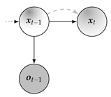
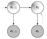
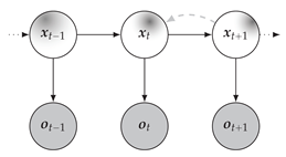
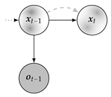
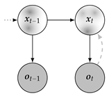
For the scope of this work, the term State Observation Model from [17] aligns best, presuming only the presence of state and observation variables. The graphical interpretation of this probabilistic model is provided in Figure 1, with arrows indicating variable dependencies, white nodes  representing hidden variables, and gray nodes
  denoting variables
with given realizations (either by observation or estimation). Distributions are visualized
as density maps
  within the respective nodes. The graph will be further extended by
  to depict likelihoods, which may be interpreted as incomplete state distributions because the encoded observation data may not be sufficient to form a full rank probabilistic description of the whole state space. Contrary to state distributions and likelihoods, state estimates will be shown as dots
  within the respective nodes.
 representing hidden variables, and gray nodes
  denoting variables
with given realizations (either by observation or estimation). Distributions are visualized
as density maps
  within the respective nodes. The graph will be further extended by
  to depict likelihoods, which may be interpreted as incomplete state distributions because the encoded observation data may not be sufficient to form a full rank probabilistic description of the whole state space. Contrary to state distributions and likelihoods, state estimates will be shown as dots
  within the respective nodes.
Figure 1.
Probabilistic graph of the state observation model.
2.1. Marginal Inference
Predicting, filtering, and smoothing all refer to inferring the marginal distribution of a specific state variable given a partial observation sequence , i.e.,
and differ only in whether observations are considered proactive (), reactive (), or retroactive (), respectively [57]. These tasks can be accomplished by marginalizing the joint posterior . Certainly, the marginals can be computed recursively, and therefore more efficiently, by utilizing the factorization (4), which exploits the sparse dependency structure of the state observation model. This paper considers only one-step predictions (), which occur in an a priori sense within filtering or smoothing. In Table 2, the marginals for are decomposed into well-known expressions mainly by applying Bayes’ theorem, the law of total probability, and by exploiting independencies. Derivations can be found in [10,65].

Table 2.
Marginal inference tasks (gray) along with substeps in state observation models.
All terms appearing in Table 2 are either model parameters (1)–(3), constant factors, or can be inferred recursively. However, smoothing can be performed by two fundamentally different approaches: recursive forward-filtering/backward-correcting, also known as fixed-lag smoothing, or non-recursive forward-filtering/backward-filtering, referred to as two-filter smoothing. Here, ‘recursive’ and ‘non-recursive’ refer to whether the smoothing marginals are inferred recursively. Therefore, the two-filter smoother is non-recursive, although it decomposes into two recursive filters, one forward in time for and the other backward in time for . The backward filter recursion is given by
Both (6) and (7) represent likelihoods. Hence, the integrals over the state variable might not always exist.
2.2. MAP Inference (Decoding)
State estimates can be decoded from the posterior marginals by maximization
While subsequent marginal distributions are coherent by transition kernel , the obtained sequences and are not coherent, and might even be invalid, e.g., if the transition probability is zero for any t. Marginal coherence does not imply MAP coherence.
One way to obtain coherent state estimates is by decoding the joint MAP assignment, i.e., maximizing the joint posterior over all possible sequences
Efficiently decoding is limited to special cases, such as HMM (Viterbi algorithm [18,20,21]) and Gaussian models (sequence of marginal means becomes the joint mode, Lemma 2). No analytical solutions are known for more general state observation models, such as mixture models.
An efficient approach to decoding coherent state sequences was recently proposed in [11]. Instead of aiming for the joint sequence (10), this approach focuses on maximizing marginal distributions similar to (9), but additionally, conditions the marginals on previously decoded MAP state estimates in a recursive manner
This method, referred to as predecessor decoding, has a complexity similar to that of posterior decoding (8) and (9), but it yields coherent estimates, a characteristic similar to sequence decoding (10). Due to its abstract definition, predecessor decoding is fundamentally applicable to general state observation models. It is important to note that the backward recursion is specified up to initialization; is not defined in (11). This introduces a degree of freedom, as (11) formally specifies a set of predecessor sequences, each sequence consisting of coherent state estimates. Any state or point of interest can be freely chosen as the initial state for the backward recursion, with different initializations producing different predecessor sequences.
As further elaborated in [60], with regard to the joint posterior , a marginal MAP becomes
a MAP predecessor maximizes
and the joint MAP sequence fulfills
In (12) past and future states are marginalized, in (15) past states are marginalized and future states are maximized, and in (16) past and future states are maximized.
Due to the properties of arg max, MAP predecessors could have also been defined via any of the equivalent formulations in (13) and (14). Due to conditional independence of and given , the predecessor expression can be further simplified. In the following sections, we omit the superfluous and apply Bayes’ rule, leading to
3. Recursive Inference in Gaussian Models
In this section we consider linear Gaussian state observation models
Assumptions (20) and (21) can equivalently be formulated in state-space representation and , with and . Parameters are grouped per time frame in the tuple
where is a (transition-) matrix, is a (process noise covariance-) matrix, is a (observation-) matrix and is a (observation noise covariance-) matrix.
In the following, the fundamental inference tasks from Section 2, are discussed for a Gaussian model (19)–(21), given initial , , a for all , and observations .
3.1. Gaussian Marginals
Under linear Gaussian model assumptions (19)–(21), the marginals remain Gaussian
Moreover, under (19)–(21), any joint distribution is also Gaussian, e.g.,
where the joint mean consists of and the block diagonal elements of the joint covariance matrix are . The recursive formulations for the parameters in (23)–(25) are provided in Table 3 and can also be found in [10,17,34,37,65]. Two-filter smoothing in Gaussian models has also been investigated [39].

Table 3.
Recursive marginal inference in Gaussian models.
3.2. Gaussian Decoding
In contrast to Section 3.1, which deals with inferring marginal state distributions (23)–(25), this section resolves predecessor decoding under Gaussian model assumptions, and discusses its relation to the other inference methods.
Theorem 1
(Gaussian Predecessor Recursion). Consider a state observation model with linear Gaussian assumptions (19)–(21). The MAP predecessor of a given can be obtained via
where , and , are the filtered and predicted mean and covariance matrix, respectively.
Proof.
Given , the predecessor distribution to be maximized by definition (11) to obtain is . Bayes’ theorem gives
The left side consists of the transition probability and the filtered marginal at time , which are both Gaussian. In the next step we apply the Gaussian refactorization lemma (GRL [41,42,53]) to this product of two Gaussians and obtain the Gaussian representations of the two terms from the right side in (28).
where
and with . The proof is concluded with
where (30) and (31) are the predicted mean and covariance matrix , respectively, as given in Table 3 or in [10,17,34,37,65]. □
Lemma 1.
Under Gaussian model assumptions (19)–(21), the set of MAP predecessor sequences comprises the joint MAP assignment.
Proof.
Decoding the MAP predecessors of a mode (or mean) effectively generates the joint MAP sequence, as detailed in Lemma 2. □
Lemma 2.
Under Gaussian model assumptions (19)–(21) and observations , the following methods yield identical results:
- (i)
- Inferring the marginal means ;
- (ii)
- Inferring the marginal MAP assignments ;
- (iii)
- Inferring the MAP predecessors of ;
- (iv)
- Inferring the joint MAP sequence .
Proof.
(i) (ii): Under assumptions (19)–(21), the marginal posteriors of each given are Gaussian . Since mode and mean are identical for normal distributions, it follows that the marginal MAP estimates are .
(i) (iii): It holds that . Note that the recursion formula for the smoothed means, see Table 3, is identical to the decoding recursion (27); the output can only differ because of different initializations. By initializing the predecessor decoder in the mean , both recursions yield identical sequences.
(i) (iv): The joint posterior corresponding to a model in which all factors are Gaussian is a Gaussian , where is the joint mean and is the joint covariance matrix. Therefore, the joint MAP estimate is . By marginalization on the joint Gaussian posterior, one sees that the joint mean is composed of the marginal means , which concludes the proof. □
Note that the equivalence of the decoding methods only holds for Gaussian models; in particular, the predecessor decoder maximizes the joint distribution (4) only in the special case where, at , it is initialized in . Starting the decoding process in a different state will result in a different sequence, as demonstrated in [11].
An interesting aspect compared to the discrete case, where the Viterbi algorithm requires keeping track of back pointers to best prior states in a separate index structure during the forward pass, is that the predecessor decoder only requires the filtered marginals, which are computed during a standard forward filter pass. Appropriately, Algorithm 1 effectively consists of a Kalman Filter on lines 3–7, which is extended to a dynamic decoder by adding a backward predecessor decoding pass on lines 11–15. By initializing per default on lines 8–10, the algorithm will decode the joint MAP sequence if not instructed otherwise.
| Algorithm 1 Filtering and Predecessor Decoding in Gaussian Models. |
▹ predicting
▹ updating
▹ decoding
|
4. Recursive Inference in Gaussian Mixture Models
In this section we assume that the factors in (4) are convex mixtures of linear Gaussians
The process parameters are stored in the tuple
Note that we do not assume stationarity, as our contributions address the general, non-stationary setting. However, in many applications, some components of (or the entire tuple) are often assumed to be stationary or are adapted only gradually over time.
4.1. Marginal Inference
In case all model factors are linear Gaussian mixtures, the predicting, filtering, and smoothing marginals also take the form of Gaussian sums:
The recursive formulations for predicted (41) and filtered (42) weights, means, and covariance matrices can be found in Table 4 and also in [11,45,46,54,62]. The undefined factor in the filtering weights is a normalizing constant, , which ensures that and need not be specified explicitly. The recursive solution to the mixture smoothing problem is elusive, as discussed in [56]. The problem is due to the presence of division by non-Gaussian densities as stated in [51], where it is proposed to perform non-recursive forward-filtering/backward-filtering for Gaussian-Sum smoothing. The two-filter approach has since been used extensively, for instance, in [52,53,54]. It is based on the decomposition
where the terms from the right side can be solved by separate filters, one running forward and the other backward in time, as illustrated in Table 4. In general, the backward filter cannot be represented in moment form, that is, in terms of the mean and covariance matrix. Instead, it is typically formulated in information form, which is why it is commonly referred to as the backward information filter. However, in certain special cases, a moment-form representation may still be possible.

Table 4.
Marginal inference in Gaussian mixture models.
The absence of a smoothing mixture recursion in the systematic approach of Table 4 (following Table 2 and Table 3) has been the main motivation for [56,57], where a closed-form solution to this problem is discussed. However, both papers are of a theoretical nature and require practical considerations such as mixture reduction before being applicable to real-world problems. The basic idea is to insert the mixture distribution before applying Bayes’ theorem, which then results in dividing by component densities rather than dividing by mixture density.
4.2. Mixture Decoding
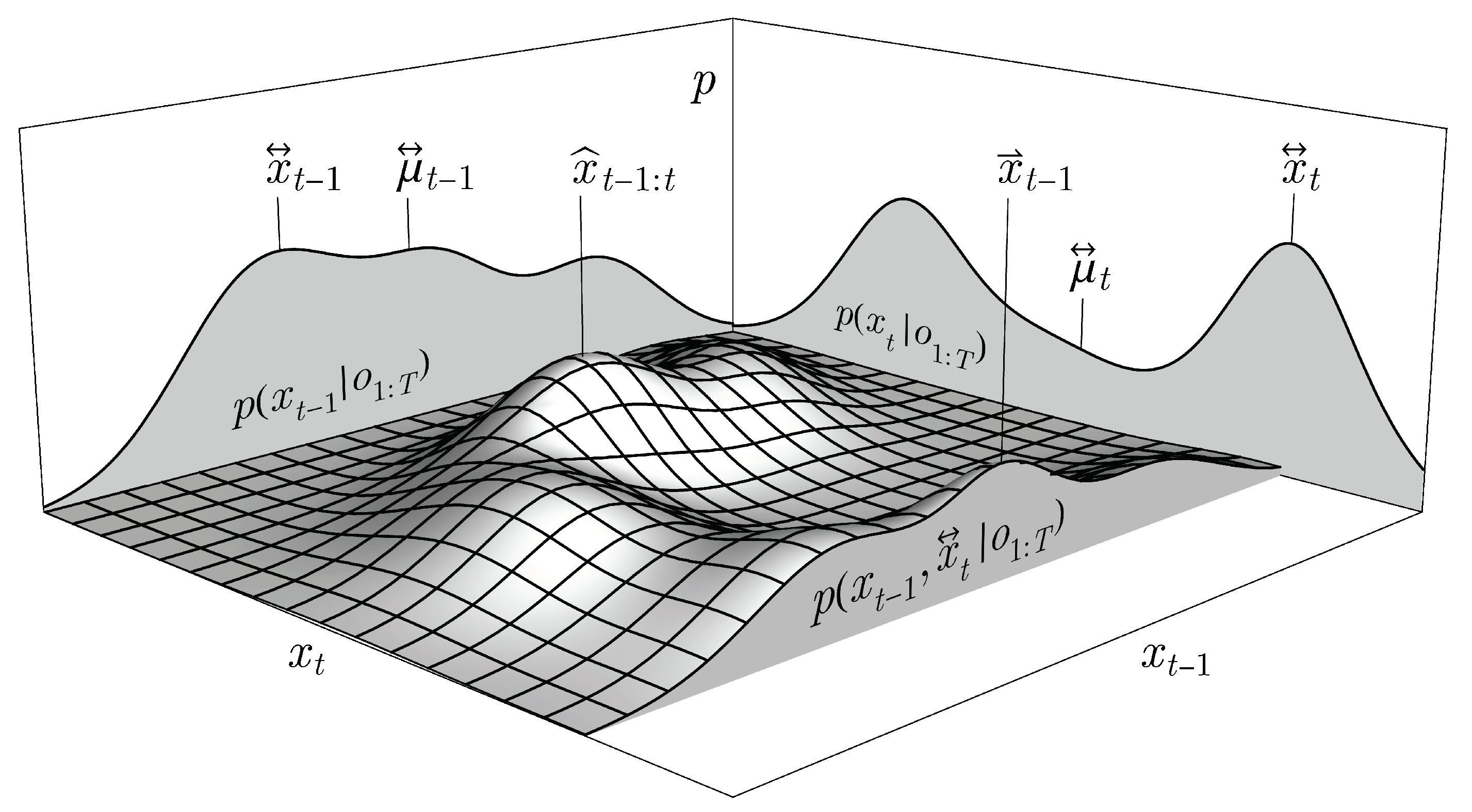
Unlike in Gaussian models, the four inference methods used to decode sequence estimates are no longer equivalent for mixture models, as demonstrated in Figure 2, which serves as a counterexample to Gaussian Lemmas 1 and 2 in the context of more general models.
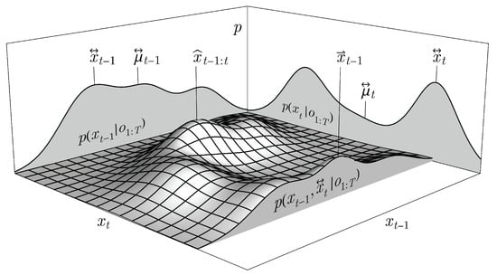
Figure 2.
Exemplary Gaussian mixture representing the joint and marginal distributions of two consecutive states and , highlighting the different state estimations of decoding marginal means , marginal MAPs , the joint MAP , and the MAP predecessor of .
Remark 1.
For general models, such as Gaussian mixture models (37)–(39), the equivalence (Lemma 2) among the decoders does not hold
as visualized in the example shown in Figure 2.
For the sake of completeness, we include the following theorem, which, in essence, was presented in [11].
Theorem 2
(Gaussian Mixture Predecessor Recursion). Consider a state observation model under the assumptions of linear Gaussian mixture model (37)–(39). The MAP predecessor of a given is
where
and with .
Proof.
The following derivation begins by noting that maximizes the distribution given in (17) and (18). It then proceeds by inserting the Gaussian mixture expressions for the transition model and the filtered marginal, combining the two sums, and finally applying the refactorization lemma to the components:
where the GRL from [41,42] was applied component-wise in (49), yielding
with . The proof is concluded with
where Table 4 or [11,45,46,54,62] give , , and . □
The appropriate predecessor decoding algorithm (Algorithm 2) consists of mixture filtering on line 2, which is followed by the dynamic mixture predecessor recursion performed on lines 3–9, starting either in a specified point of interest or in the marginal MAP (per default). Similar to mixture predicting and updating (Table 4) the double-sums in (45) are reformulated into equivalent single-sum representations (line 7) by re-indexing the components over , which then goes from 1 to . Finally, a mixture reduction is performed on line 10.
From a purely theoretical perspective, the reduction step on line 10 is optional. However, in practical Bayesian inference applications involving mixture distributions, reduction is both necessary and standard, as the number of components would otherwise increase exponentially. As discussed in [45,46], the weights associated with numerous components become negligible, allowing for their exclusion without introducing significant error. Additionally, components tend to converge to similar values, facilitating their combination. Extensive research has been conducted based on this prune and merge paradigm to reduce the number of components while maintaining a high level of approximation. One widely used reduction technique involves computing pairwise similarities based on the Kullback-Leibler divergence [54,62]. Alternative reduction methods can be found in [63,64]. In any case, the reduced Gaussian mixture should consist of fewer components, i.e., , where may be treated as a design parameter.
| Algorithm 2 Filtering and Predecessor Decoding in Gaussian Mixture Models. |
▹ mixture filtering
▹ mixture decoding
▹ mixture reduction
|
The problem of maximizing multivariate Gaussian mixtures, also known as mode finding, has received comparatively limited attention in the literature. This task can be addressed using iterative numerical methods [66,67,68], or alternatively, by selecting the most probable component mean as a greedy approximation [69,70]. Consequently, in contrast to the Gaussian case, Bayesian inference involving mixture distributions can only be performed approximately. In addition to the reduction of Gaussian mixtures on line 10, their maximization, on lines 4 and 8 in Algorithm 2, may also result in the introduction of approximation errors.
Algorithms 1 (GaussDecode()) and 2 (MixDecode()) are designed for real-time applications that aim to dynamically decode coherent state trajectories with each new observation . As , it may be necessary to consider early stopping of the decoding recursions. A potential criterion for stopping could involve detecting when the current predecessor sequence closely approaches a previously decoded sequence. A thorough convergence analysis could be the focus of future work. For offline applications, where a finite observation sequence is given from the outset, the best practice is to run the forward filtering pass and the backward decoding pass separately.
5. Quantum-Based Inference
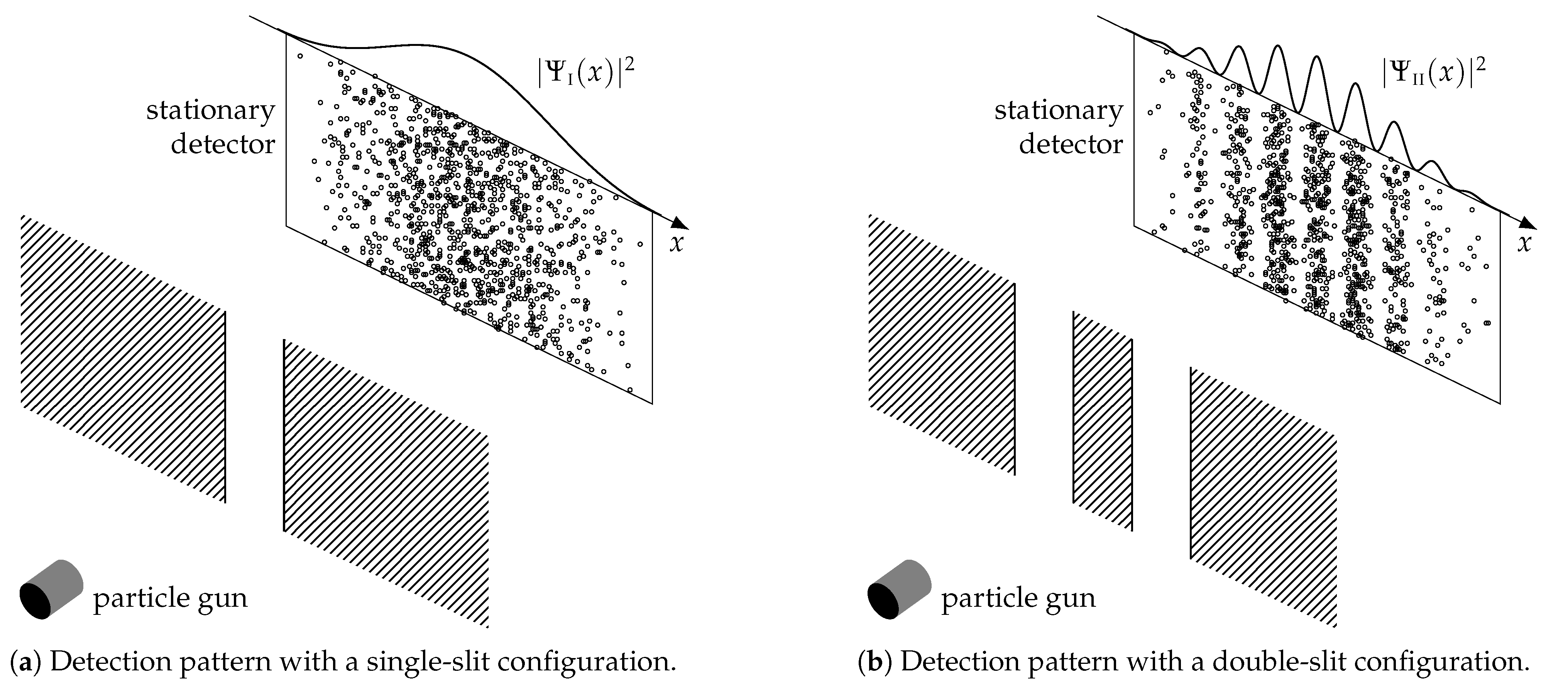
This section provides a comparative analysis of the discussed decoders. By utilizing the distinct detection patterns observed in the single- and double-slit experiments (Figure 3), we aim to infer the lateral movement of a non-stationary detector. The double-slit experiment, first conducted by Thomas Young in 1801, is one of the most famous experiments in the history of physics, providing critical insights into the nature of light and matter. The original experiment involved a light source shining through two closely spaced slits, producing an interference pattern on a stationary detector placed behind the slits. This pattern, with alternating bright and dark bands, indicated a wave-like nature of light. The experiment has been extended to particles, such as electrons, revealing that the wave-particle duality extends beyond just light and challenges classical notions of physics [12,13,14].
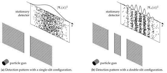
Figure 3.
Slit experiments and interference patterns with stationary detectors.
In this paper, we do not engage in the philosophical discussion regarding the underlying reasons for the occurrence of interference patterns; rather, we only presume their presence for the simulation experiment discussed in this section. The manifestation of interference patterns has been repeatedly shown through numerous experiments using various slit configurations and different quantum particles, including atoms and some molecules. The analytical form of the detection patterns has also been studied, for instance, in [15,71]. These forms emerge from applying the Born rule to the wavefunction [12]. For the slit experiments specifically, consists of sinc- and cos-terms accounting for diffraction and interference effects, respectively, and is parameterized by wavenumber k or wavelength , slit width a, slit separation d, and slit-to-detector distance ℓ. Noteworthy, the detection pattern of the double-slit has a single-slit envelope. We will consider experiments with setup
The wavenumber k in (50) corresponds to electrons with a kinetic energy of , which have a de Broglie wavelength of approximately .
Contrary to the classical experiment, we simulate a detector non-stationary in x-direction, with the aim of inferring its lateral movement from sequential quantum particle detections. The state variable is , where x is the lateral position and v the velocity. In the following we formulate appropriate state observation models and evaluate the different inference and decoding methods on simulated data.
5.1. Observation Models
Since the analytic forms of the detection patterns are well known, we use a model-based approach to approximate and by appropriate Gaussian and Gaussian mixture pdf’s, respectively. The single-slit pattern is approximated by a Gaussian
with stationary parameters
The detection pattern for the double-slit is approximated by a Gaussian mixture
with a total number of components, and
where normalizes the weights such that . Again, all parameters are stationary. The terms for the standard deviations and were determined by Taylor expansion and curvature matching. The mixture components were additionally narrowed such that the minima approach zero; this was achieved by specifying a coefficient <1 of inside the covariance matrix in (54).
For a fair comparison with the uni-modal Gaussian approximation, the component number for the multi-modal mixture was set to (), ignoring diffraction effects, occurring at much lower magnitude and further beyond the range shown in Figure 3, yet indicated in Figure 4. Increasing would generate components at distant diffraction maxima, leading to more accurate approximations.

Figure 4.
Gaussian mixture approximations (dashed) of interference patterns (solid).
Note that the inference methods are not limited to the presented approximations; in particular, they are not restricted to model-based approximations. When actual detection data is available, data-driven approximations can be employed. However, the model-based approximations in (52) and (54) offer the advantage of scaling appropriately with the parameters of the experimental setup (50).
In the slit experiments, the likelihoods and may be interpreted as reconstruction-attempts of possible quantum waveforms and , before they collapsed into the particle observation o.
5.2. Transition Model and Initialization
We consider inferring the sequence of positions and velocities of an object (detector) from a sequence of noisy position observations . For the transition model, we specify that the motion of the object retains a constant velocity over the interval between two time steps but can experience a random acceleration with standard deviation . Hence, we set , i.e., a linear Gaussian with stationary parameters
specifying and . The initial state was with
5.3. Evaluation and Implementation
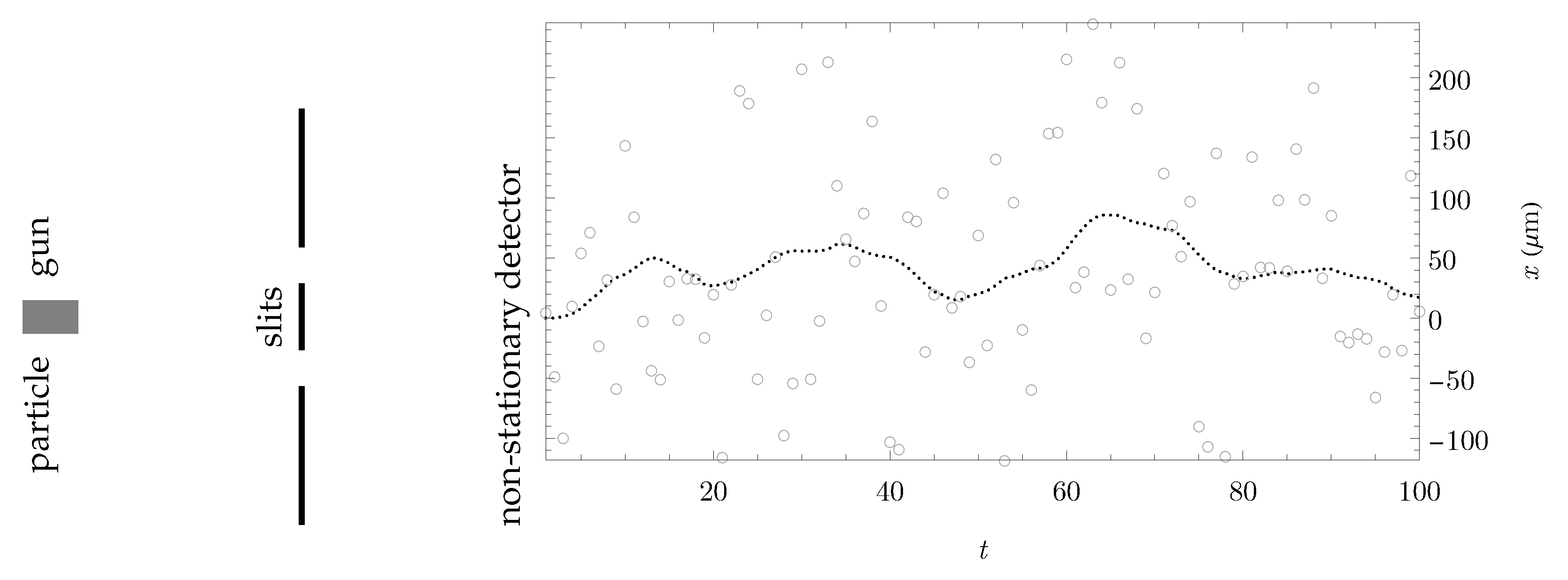
Having specified the observation models, the transition model, and the initial state distribution, we can sample a trajectory that constitutes the hidden ground truth, along with corresponding observations. A sample trajectory , together with the associated double-slit detection samples , is shown in Figure 5, featuring an absolute distance traveled of .
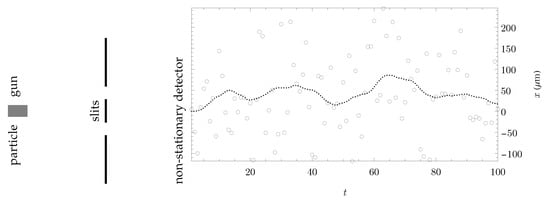
Figure 5.
Double-slit experiment with a non-stationary detector. The simulated hidden ground truth of the 1D-movement is shown as a dotted line with double-slit detections as gray circles.
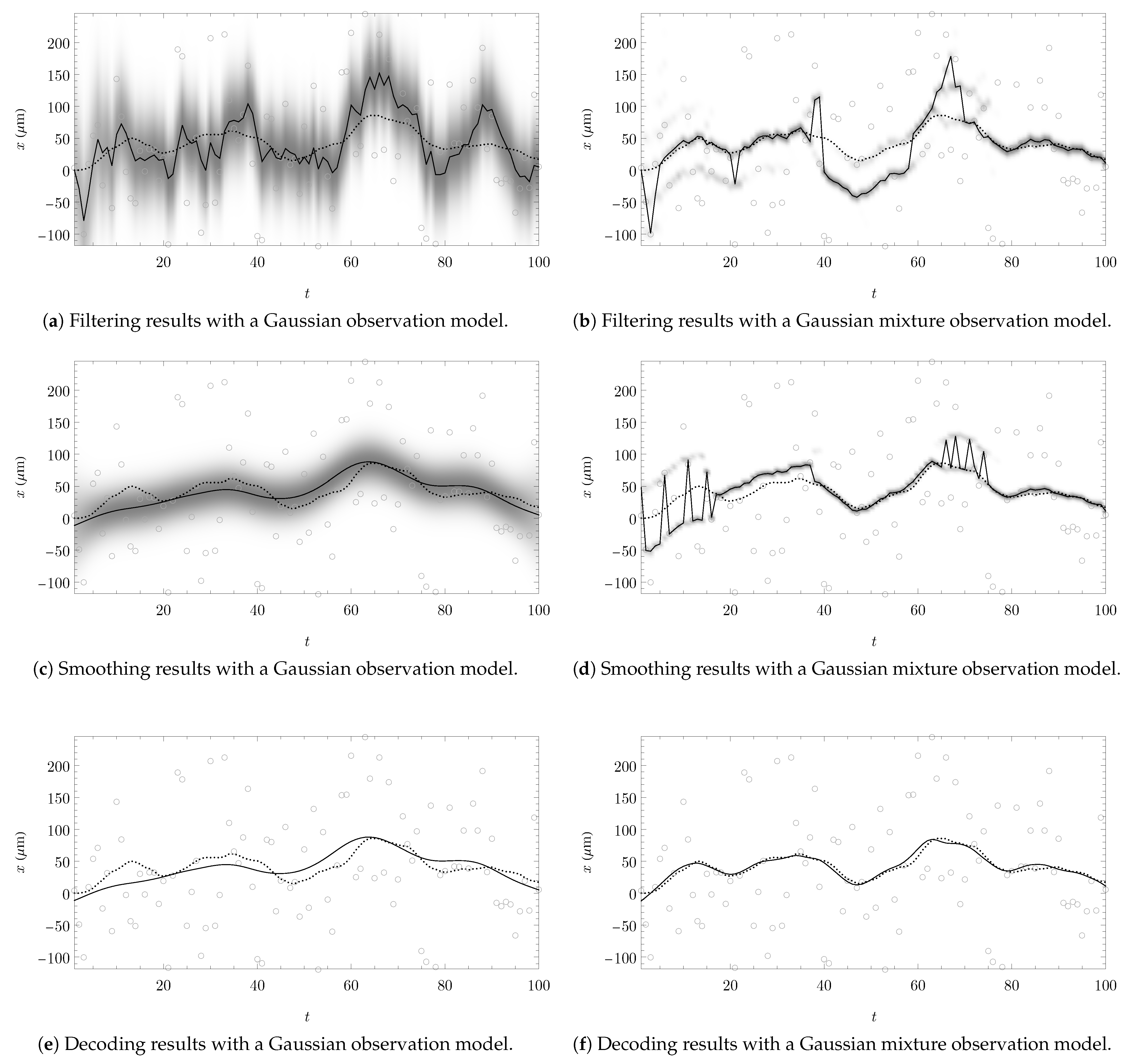
All data and parameters required to perform Bayesian inference evaluations have now been specified. The evaluation results, illustrated in Figure 6, are based primarily on straightforward implementations of the recursive marginal inference methods from Table 3 and Table 4, and of the recursive MAP inferences methods GaussDecode() and MixDecode() from Algorithms 1 and 2, respectively. For the implementation of an accurate two-filter smoother, the results of which are shown in Figure 6d, we refer to [54].

Figure 6.
Inference results under Gaussian model or one-slit assumptions (a,c,e) and under Gaussian mixture model or double-slit assumptions (b,d,f). The ground truth trajectory is dotted, gray circles indicate the observations, and distributions are plotted in gray scale for each t. Trajectory estimates (solid black lines) are obtained by posterior decoding, i.e., maximizing the marginal distributions in (a–d), respectively by predecessor decoding in (e,f).
To prevent exponential growth in the number of mixture components, a reduction technique was applied to each filtered and smoothed distribution. This was achieved by pruning components with weights below a certain threshold (i.e., and ), followed by merging similar components based on the Bhattacharyya distance [61]. Each mixture was limited to at most components. Mixture maximization was implemented by selecting the component mean with the highest probability. Note that this technique may perform poorly if the components are clustered rather than sparse. In such cases, we recommend initializing gradient-based optimization or hill-climbing techniques at each component mean.
While the specific mixture reduction or maximization technique is not critical, it is important for the comparison to apply the same techniques consistently across all Bayesian inference methods. Compared to Gaussian filtering, -smoothing, -decoding, and -mixture decoding, which had negligible computation time, the evaluation of mixture filtering and smoothing required a few seconds per run, primarily due to the computation of pairwise component distances in the mixture reduction step. All computations were performed on a business-grade notebook.
6. Discussion
The evaluation results shown in Figure 6 illustrate the different characteristics of the individual inference methods. Filtering (Figure 6a,b) is more prone to errors in the observation data, as marginals only depend on previous observations. Smoothing (Figure 6c,d) is based on previous and future observations, the smoothed distributions are more compact, and estimation outliers are largely eliminated. Predecessor decoding (Figure 6e,f) utilizes previous observations and future state estimates, resulting in more plausible sequences that better reflect the assumed transition behavior. In the context of the quantum-based tracking example, this improvement is reflected in the distance error, defined as the difference between the estimated distance traveled and the true distance traveled, which amounts to
- for Gaussian filtered (Figure 6a);
- for Mixture filtered (Figure 6b);
- for Mixture smoothed (Figure 6d);
- Only for the Mixture decoded trajectory (Figure 6f).
Under non-Gaussian conditions, only the predecessor decoder was able to generate coherent state estimates and plausible sequences. This is more significantly demonstrated in the distance error distribution charts shown in Figure 7b.

Figure 7.
Error statistics for all inference methods based on 10,000 evaluation rounds.
While Figure 6 illustrates one evaluation round, the error statistics in Figure 7 and Figure 8 are based on 10,000 evaluation rounds, where in each round, the ground truth trajectory and associated double-slit observations were sampled randomly according to the specified model. The filtering methods have relatively poor error statistics, in particular with regard to the distance error. Gaussian smoothing and Gaussian decoding perform identically as both were initialized identically in each round. Mixture filtering, smoothing, and decoding have comparable good position accuracies. However, with mixture filtering and smoothing, the distance error accumulates significantly over time, whereas the decoder strictly acts according to the transition model and produces coherent state estimates, resulting in low distance errors. The relatively reasonable performance of the (single) Gaussian decoder and smoother can be attributed to the fact that, in the considered experiment, the mixture (double-slit) components are enveloped by a Gaussian-like (single-slit) function.
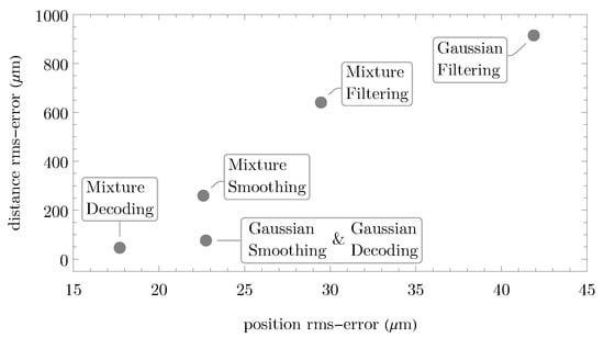
Figure 8.
RMSE diagram comparing all inference methods based on 10,000 evaluation rounds.
Note that both Gaussian and mixture-based inference methods were evaluated on double-slit observation data. We deliberately omitted separate sampling of single-slit observation data to enable direct comparability. However, the comparison presented in Figure 6, Figure 7 and Figure 8 can be interpreted not only as a contrast between Gaussian and mixture-based inference but also as a comparison between classical and quantum-based inference and, finally, between single- vs. double-slit-based inference:
- Gaussian vs. Mixture Model is the destined and mathematically motivated interpretation, highlighting the behavior induced by the models across the discussed inference methods. The Gaussian model constitutes an oversimplification; in particular, Gaussian distributions are underfitting the double-slit pattern. In contrast, the more complex Gaussian mixture model reduces the model error (bias) by better capturing the interference sub-patterns.
- Classical vs. Quantum Particles is an applicable interpretation for the considered experiment setup. For classical or real particles, the expected detection pattern in a double-slit experiment would form a bimodal mixture. However, because the distance between the two slits is small relative to the detector distance, the resulting modes would significantly overlap, effectively resembling a single Gaussian. Thus, the single Gaussian model approximates the classical outcome, supporting this interpretation. But beware of the counterintuitive nature of the subject: If we try to gather additional information about the particle, e.g., by sensing through which slit it went, then this would slightly improve the accuracy with real particles but increase the uncertainty with quantum particles, as the observation at the slit instantly collapses the waveform such that we cannot exploit interference patterns at the detector.
- Single vs. Double-Slit interpretation of the comparison for quantum particles remains reasonable, as the double-slit pattern is enveloped by a single-slit profile and as the specified mixture approximation preserves symmetry. Whether and how the addition of more slits, leading to more complex interference patterns, improves the inference results remains an open question.
The results indicate that mixture-based inference methods can efficiently exploit the fundamental uncertainty of the state of quantum particles to increase the certainty of states of a real object, e.g., the movement of a non-stationary detector sensing double-slit observations. This study was conducted entirely through simulation, and the results strongly support the effectiveness of the mixture-based predecessor decoder in particular. While these findings are promising, they remain theoretical in nature. As such, experimental validation is an essential next step to assess the practical applicability and robustness of these methods in real-world physical systems. Unfortunately, the authors are no experts in this field and would encourage quantum physicists and experimental researchers to investigate these results further through empirical studies and laboratory experiments. If the quantum interpretations are deemed inapplicable for any reason, the results should be considered solely in the fallback Gaussian vs. Mixture Model interpretation.
In essence, the double-slit experiment, with its multimodal interference patterns, served as an exemplary demonstration for showcasing the potential of the recursive Bayesian decoder. Further applications of this method, particularly in signal processing, are under consideration and will be explored in future work.
General Discussion and Conclusions
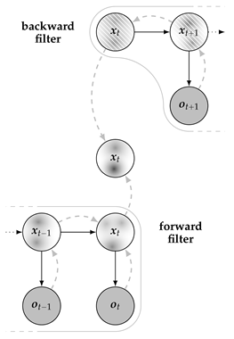
Decoding MAP predecessors has a comparable complexity to decoding marginal MAP assignments since both methods maximize marginal state distributions. However, by conditioning each marginal on the previously decoded estimate during the backward recursion, predecessor decoding achieves coherent estimates, a characteristic akin to the joint MAP. It has been reasoned that predecessor decoding, being relatively new, has not yet been thoroughly discussed in the literature. One reason is that recursive smoothing in Gaussian models already yields the joint (and thus coherent) MAP assignment, spoiling the contributions of another such decoder. Another important reason is that, until recently, no analytic solution existed for recursive smoothing in mixture models (see [56]). In the context of mixture models, neither the recursive nor the non-recursive two-filter smoother produces the joint MAP, unlike in the case of Gaussian models. However, the process of recursively decoding the MAP predecessors constitutes the MAP inference analog to the marginal inference task of recursive smoothing. This analogy becomes apparent in Figure 9 in a side-by-side comparison of the graphical interpretations of both methods. Finally, we note that backward decoding seamlessly integrates with forward filtering, making it inherently applicable wherever a Bayesian filter is utilized.

Figure 9.
Analogous inference graphs of recursive smoothing and recursive predecessor decoding.
Author Contributions
Conceptualization, B.R.; methodology, B.R.; software, B.R.; validation, B.R., D.E. and M.P.-S.; formal analysis, B.R. and D.E.; investigation, B.R.; resources, M.P.-S.; writing—original draft preparation, B.R.; writing—review and editing, B.R., M.P.-S. and D.E.; visualization, B.R.; supervision, D.E.; project administration, M.P.-S.; funding acquisition, M.P.-S. All authors have read and agreed to the published version of the manuscript.
Funding
This work has been supported by the COMET-K2 Center of the Linz Center of Mechatronics (LCM) funded by the Austrian federal government and the federal state of Upper Austria.
Data Availability Statement
Only reproducible simulation data was created and analyzed in this study. All simulation setups are explained in detail.
Conflicts of Interest
Branislav Rudić and Markus Pichler-Scheder were employed by Linz Center of Mechatronics GmbH. The remaining authors declare that the research was conducted in the absence of any commercial or financial relationships that could be construed as a potential conflict of interest.
References
- Abdallah, M.A. Advancing Decision-Making in AI Through Bayesian Inference and Probabilistic Graphical Models. Symmetry 2025, 17, 635. [Google Scholar] [CrossRef]
- Yang, Z.; Zhang, X.; Xiang, W.; Lin, X. A Novel Particle Filter Based on One-Step Smoothing for Nonlinear Systems with Random One-Step Delay and Missing Measurements. Sensors 2025, 25, 318. [Google Scholar] [CrossRef] [PubMed]
- Ali, W.; Li, Y.; Chen, Z.; Raja, M.A.Z.; Ahmed, N.; Chen, X. Application of Spherical-Radial Cubature Bayesian Filtering and Smoothing in Bearings Only Passive Target Tracking. Entropy 2019, 21, 1088. [Google Scholar] [CrossRef]
- Cassidy, M.J.; Penny, W.D. Bayesian nonstationary autoregressive models for biomedical signal analysis. IEEE Trans. Biomed. Eng. 2002, 49, 1142–1152. [Google Scholar] [CrossRef]
- Behnamfar, F.; Alajaji, F.; Linder, T. MAP decoding for multi-antenna systems with non-uniform sources: Exact pairwise error probability and applications. IEEE Trans. Commun. 2009, 57, 242–254. [Google Scholar] [CrossRef]
- Gao, Y.; Tang, X.; Li, T.; Chen, Q.; Zhang, X.; Li, S.; Lu, J. Bayesian Filtering Multi-Baseline Phase Unwrapping Method Based on a Two-Stage Programming Approach. Appl. Sci. 2020, 10, 3139. [Google Scholar] [CrossRef]
- Retkute, R.; Thurston, W.; Gilligan, C.A. Bayesian Inference for Multiple Datasets. Stats 2024, 7, 434–444. [Google Scholar] [CrossRef]
- Huang, Z.; Sarovar, M. Smoothing of Gaussian quantum dynamics for force detection. Phys. Rev. A 2018, 97, 042106. [Google Scholar] [CrossRef]
- Ma, K.; Kong, J.; Wang, Y.; Lu, X.M. Review of the Applications of Kalman Filtering in Quantum Systems. Symmetry 2022, 14, 2478. [Google Scholar] [CrossRef]
- Särkkä, S. Bayesian Filtering and Smoothing; Institute of Mathematical Statistics Textbooks; Cambridge University Press: Cambridge, UK, 2013. [Google Scholar] [CrossRef]
- Rudić, B.; Pichler-Scheder, M.; Efrosinin, D. Valid Decoding in Gaussian Mixture Models. In Proceedings of the 2024 IEEE 3rd Conference on Information Technology and Data Science (CITDS), Debrecen, Hungary, 26–28 August 2024. [Google Scholar] [CrossRef]
- Griffiths, D.J.; Schroeter, D.F. The Wave Function. In Introduction to Quantum Mechanics; Cambridge University Press: Cambridge, UK, 2018; pp. 3–24. [Google Scholar]
- Feynman, R.P.; Leighton, R.B.; Sands, M. The Feynman Lectures on Physics, Vol. III: The New Millennium Edition: Quantum Mechanics; The Feynman Lectures on Physics; Basic Books: New York, NY, USA, 2011. [Google Scholar]
- Cohen-Tannoudji, C.; Diu, B.; Laloë, F. Quantum Mechanics, 2nd ed.; Wiley-VCH: Weinheim, Germany, 2019; Volume 1–3. [Google Scholar]
- Rolleigh, R. The Double Slit Experiment and Quantum Mechanics. In Hendrix College Faculty Archives; Hendrix College: Conway, AR, USA, 2010. [Google Scholar]
- Dodonov, V.V.; Man’ko, M.A. CAMOP: Quantum Non-Stationary Systems. Phys. Scr. 2010, 82, 031001. [Google Scholar] [CrossRef]
- Koller, D.; Friedman, N. Probabilistic Graphical Models: Principles and Techniques; Adaptive Computation and Machine Learning; The MIT Press: Cambridge, MA, USA, 2009. [Google Scholar]
- Rabiner, L.R. A tutorial on hidden Markov models and selected applications in speech recognition. Proc. IEEE 1989, 77, 257–286. [Google Scholar] [CrossRef]
- Cappé, O.; Moulines, E.; Rydén, T. Filtering and Smoothing Recursions. In Inference in Hidden Markov Models; Springer: New York, NY, USA, 2005; pp. 51–76. [Google Scholar] [CrossRef]
- Viterbi, A.J. Error bounds for convolutional codes and an asymptotically optimum decoding algorithm. IEEE Trans. Inf. Theory 1967, 13, 260–269. [Google Scholar] [CrossRef]
- Forney, G.D. The Viterbi algorithm. Proc. IEEE 1973, 61, 268–278. [Google Scholar] [CrossRef]
- Zegeye, W.K.; Dean, R.A.; Moazzami, F. Multi-Layer Hidden Markov Model Based Intrusion Detection System. Mach. Learn. Knowl. Extr. 2019, 1, 265–286. [Google Scholar] [CrossRef]
- Rudić, B.; Pichler-Scheder, M.; Efrosinin, D.; Putz, V.; Schimbäck, E.; Kastl, C.; Auer, W. Discrete- and Continuous-State Trajectory Decoders for Positioning in Wireless Networks. IEEE Trans. Instrum. Meas. 2020, 69, 6016–6029. [Google Scholar] [CrossRef]
- Arulampalam, M.S.; Maskell, S.; Gordon, N.; Clapp, T. A tutorial on particle filters for online nonlinear/non-Gaussian Bayesian tracking. IEEE Trans. Signal Process. 2002, 50, 174–188. [Google Scholar] [CrossRef]
- Kotecha, J.; Djuric, P. Gaussian sum particle filtering. IEEE Trans. Signal Process. 2003, 51, 2602–2612. [Google Scholar] [CrossRef]
- Godsill, S.; Doucet, A.; West, M. Maximum a Posteriori Sequence Estimation Using Monte Carlo Particle Filters. Ann. Inst. Stat. Math. 2001, 53, 82–96. [Google Scholar] [CrossRef]
- Godsill, S.; Doucet, A.; West, M. Monte Carlo Smoothing for Nonlinear Time Series. J. Am. Stat. Assoc. 2004, 99, 156–168. [Google Scholar] [CrossRef]
- Mejari, M.; Piga, D. Maximum—A Posteriori Estimation of Linear Time-Invariant State-Space Models via Efficient Monte-Carlo Sampling. ASME Lett. Dyn. Syst. Control 2021, 2, 011008. [Google Scholar] [CrossRef]
- Klaas, M.; Briers, M.; de Freitas, N.; Doucet, A.; Maskell, S.; Lang, D. Fast particle smoothing: If I had a million particles. In Proceedings of the 23rd International Conference on Machine Learning (ICML ’06), New York, NY, USA, 25–29 June 2006; pp. 481–488. [Google Scholar] [CrossRef]
- Doucet, A.; Johansen, A.M. A Tutorial on Particle Filtering and Smoothing: Fifteen Years Later. In The Oxford Handbook of Nonlinear Filtering; Crisan, D., Rozovsky, B., Eds.; Oxford University Press: Oxford, UK, 2011; pp. 656–704. [Google Scholar]
- Daum, F.E.; Huang, J. Curse of dimensionality and particle filters. In Proceedings of the 2003 IEEE Aerospace Conference Proceedings (Cat. No. 03TH8652), Big Sky, MT, USA, 8–15 March 2003; Volume 4, pp. 1979–1993. [Google Scholar]
- Lolla, T.; Lermusiaux, P.F.J. A Gaussian Mixture Model Smoother for Continuous Nonlinear Stochastic Dynamical Systems: Theory and Scheme. Mon. Weather Rev. 2017, 145, 2743–2761. [Google Scholar] [CrossRef]
- van Leeuwen, P.J.; Künsch, H.R.; Nerger, L.; Potthast, R.; Reich, S. Particle filters for high-dimensional geoscience applications: A review. Q. J. R. Meteorol. Soc. 2019, 145, 2335–2365. [Google Scholar] [CrossRef]
- Kalman, R.E. A New Approach to Linear Filtering and Prediction Problems. Trans. ASME- Basic Eng. 1960, 82, 35–45. [Google Scholar] [CrossRef]
- Smith, G.L.; Schmidt, S.F.; McGee, L.A. Application of Statistical Filter Theory to the Optimal Estimation of Position and Velocity on Board a Circumlunar Vehicle; NASA Technical Report; National Aeronautics and Space Administration: Washington, DC, USA, 1962.
- Julier, S.J.; Uhlmann, J.K. New extension of the Kalman filter to nonlinear systems. In Proceedings of the Signal Processing, Sensor Fusion, and Target Recognition VI, Orlando, FL, USA, 21–25 April 1997; SPIE: Bellingham, MA, USA, 1997; Volume 3068, pp. 182–193. [Google Scholar] [CrossRef]
- Rauch, H.E.; Tung, F.; Striebel, C.T. Maximum likelihood estimates of linear dynamic systems. AIAA J. 1965, 3, 1445–1450. [Google Scholar] [CrossRef]
- Särkkä, S. Unscented Rauch–Tung–Striebel Smoother. IEEE Trans. Autom. Control 2008, 53, 845–849. [Google Scholar] [CrossRef]
- Fraser, D.C.; Potter, J.E. The optimum linear smoother as a combination of two optimum linear filters. IEEE Trans. Autom. Control 1969, 14, 387–390. [Google Scholar] [CrossRef]
- Cosme, E.; Verron, J.; Brasseur, P.; Blum, J.; Auroux, D. Smoothing Problems in a Bayesian Framework and their Linear Gaussian Solutions. Mon. Weather Rev. 2012, 140, 683–695. [Google Scholar] [CrossRef]
- Ainsleigh, P.L. Theory of Continuous-State Hidden Markov Models and Hidden Gauss-Markov Models; Technical Report 11274; Naval Undersea Warfare Cent.: Newport, RI, USA, 2001. [Google Scholar]
- Ainsleigh, P.L.; Kehtarnavaz, N.; Streit, R.L. Hidden Gauss-Markov models for signal classification. IEEE Trans. Signal Process. 2002, 50, 1355–1367. [Google Scholar] [CrossRef]
- Turin, W. Continuous State HMM. In Performance Analysis and Modeling of Digital Transmission Systems; Springer: Boston, MA, USA, 2004; Chapter 7; pp. 295–340. [Google Scholar] [CrossRef]
- Ortiz, J.; Evans, T.; Davison, A.J. A visual introduction to Gaussian Belief Propagation. arXiv 2021, arXiv:2107.02308. [Google Scholar]
- Sorenson, H.W.; Alspach, D.L. Recursive Bayesian Estimation using Gaussian Sums. Automatica 1971, 7, 465–479. [Google Scholar] [CrossRef]
- Alspach, D.L.; Sorenson, H.W. Nonlinear Bayesian estimation using Gaussian sum approximations. IEEE Trans. Autom. Control 1972, 17, 439–448. [Google Scholar] [CrossRef]
- Anderson, B.D.; Moore, J.B. Gaussian Sum Estimators. In Optimal Filtering; Kailath, T., Ed.; Information and System Sciences Series; Prentice-Hall: Saddle River, NJ, USA, 1979; pp. 211–222. [Google Scholar]
- Terejanu, G.; Singla, P.; Singh, T.; Scott, P.D. Adaptive Gaussian Sum Filter for Nonlinear Bayesian Estimation. IEEE Trans. Autom. Control 2011, 56, 2151–2156. [Google Scholar] [CrossRef]
- Horwood, J.T.; Aragon, N.D.; Poore, A.B. Gaussian Sum Filters for Space Surveillance: Theory and Simulations. J. Guid. Control. Dyn. 2011, 34, 1839–1851. [Google Scholar] [CrossRef]
- Šimandl, M.; Královec, J. Filtering, Prediction and Smoothing with Gaussian Sum Representation. IFAC Proc. Vol. 2000, 33, 1157–1162. [Google Scholar] [CrossRef]
- Kitagawa, G. The two-filter formula for smoothing and an implementation of the Gaussian-sum smoother. Ann. Inst. Stat. Math. 1994, 46, 605–623. [Google Scholar] [CrossRef]
- Kitagawa, G. Revisiting the Two-Filter Formula for Smoothing for State-Space Models. arXiv 2023, arXiv:2307.03428. [Google Scholar]
- Vo, B.N.; Vo, B.T.; Mahler, R.P.S. Closed-Form Solutions to Forward–Backward Smoothing. IEEE Trans. Signal Process. 2012, 60, 2–17. [Google Scholar] [CrossRef]
- Balenzuela, M.P.; Dahlin, J.; Bartlett, N.; Wills, A.G.; Renton, C.; Ninness, B. Accurate Gaussian Mixture Model Smoothing using a Two-Filter Approach. In Proceedings of the 2018 IEEE Conference on Decision and Control (CDC), Miami, FL, USA, 17–19 December 2018; pp. 694–699. [Google Scholar] [CrossRef]
- Balenzuela, M.P.; Wills, A.G.; Renton, C.; Ninness, B. A new smoothing algorithm for jump Markov linear systems. Automatica 2022, 140, 110218. [Google Scholar] [CrossRef]
- Rudić, B.; Sturm, V.; Efrosinin, D. On the Analytic Solution to Recursive Smoothing in Mixture Models. In Proceedings of the 2024 58th Asilomar Conference on Signals, Systems, and Computers, Pacific Grove, CA, USA, 27–30 October 2024; pp. 1301–1305. [Google Scholar] [CrossRef]
- Rudić, B.; Sturm, V.; Efrosinin, D. Recursive Bayesian Smoothing with Gaussian Sums. TechRxiv 2025. preprint. [Google Scholar] [CrossRef]
- Cedeño, A.L.; González, R.A.; Godoy, B.I.; Carvajal, R.; Agüero, J.C. On Filtering and Smoothing Algorithms for Linear State-Space Models Having Quantized Output Data. Mathematics 2023, 11, 1327. [Google Scholar] [CrossRef]
- Rudić, B.; Pichler-Scheder, M.; Efrosinin, D. Maximum A Posteriori Predecessors in State Observation Models. In Proceedings of the 23rd International Conference on Information Technologies and Mathematical Modelling (ITMM’2024), Karshi, Usbekistan, 20–26 October 2024; pp. 391–395. [Google Scholar]
- Rudić, B.; Sturm, V.; Efrosinin, D. On Recursive Marginal and MAP Inference in State Observation Models. In Information Technologies and Mathematical Modelling. Queueing Theory and Related Fields; Dudin, A., Nazarov, A., Moiseev, A., Eds.; Springer: Cham, Switzerland, 2025; pp. 85–97. [Google Scholar] [CrossRef]
- Hennig, C. Methods for merging Gaussian mixture components. Adv. Data Anal. Classif. 2010, 4, 3–34. [Google Scholar] [CrossRef]
- Wills, A.G.; Hendriks, J.; Renton, C.; Ninness, B. A Bayesian Filtering Algorithm for Gaussian Mixture Models. arXiv 2017. [Google Scholar] [CrossRef]
- Crouse, D.F.; Willett, P.; Pattipati, K.; Svensson, L. A look at Gaussian mixture reduction algorithms. In Proceedings of the 14th International Conference on Information Fusion, Chicago, IL, USA, 5–8 July 2011; pp. 1–8. [Google Scholar]
- Ardeshiri, T.; Granström, K.; Özkan, E.; Orguner, U. Greedy Reduction Algorithms for Mixtures of Exponential Family. IEEE Signal Process. Lett. 2015, 22, 676–680. [Google Scholar] [CrossRef]
- Einicke, G.A. Smoothing, Filtering and Prediction: Estimating the Past, Present and Future, 2nd ed.; Prime Publishing: Northbrook, IL, USA, 2019. [Google Scholar]
- Carreira-Perpiñán, M.Á. Mode-finding for mixtures of Gaussian distributions. IEEE Trans. Pattern Anal. Mach. Intell. 2000, 22, 1318–1323. [Google Scholar] [CrossRef]
- Carreira-Perpiñán, M.Á. A review of mean-shift algorithms for clustering. arXiv 2015, arXiv:1503.00687. [Google Scholar]
- Pulkkinen, S.; Mäkelä, M.M.; Karmitsa, N. A Continuation Approach to Mode-Finding of Multivariate Gaussian Mixtures and Kernel Density Estimates. J. Glob. Optim. 2013, 56, 459–487. [Google Scholar] [CrossRef]
- Olson, E.; Agarwal, P. Inference on Networks of Mixtures for Robust Robot Mapping. In Robotics: Science and Systems VIII; The MIT Press: Cambridge, MA, USA, 2013; pp. 313–320. [Google Scholar] [CrossRef]
- Pfeifer, T.; Lange, S.; Protzel, P. Advancing Mixture Models for Least Squares Optimization. IEEE Robot. Autom. Lett. 2021, 6, 3941–3948. [Google Scholar] [CrossRef]
- Luo, B.J.; Francis, L.; Rodríguez-Fajardo, V.; Galvez, E.J.; Khoshnoud, F. Young’s double-slit interference demonstration with single photons. Am. J. Phys. 2024, 92, 308–316. [Google Scholar] [CrossRef]
Disclaimer/Publisher’s Note: The statements, opinions and data contained in all publications are solely those of the individual author(s) and contributor(s) and not of MDPI and/or the editor(s). MDPI and/or the editor(s) disclaim responsibility for any injury to people or property resulting from any ideas, methods, instructions or products referred to in the content. |
© 2025 by the authors. Licensee MDPI, Basel, Switzerland. This article is an open access article distributed under the terms and conditions of the Creative Commons Attribution (CC BY) license (https://creativecommons.org/licenses/by/4.0/).


