Existence of Local Solutions to a Free Boundary Problem for Compressible Viscous Magnetohydrodynamics

Abstract

The motion of viscous compressible magnetohydrodynamics (MHD) is considered in a domain bounded by a free boundary. The motion interacts through the free surface with an electromagnetic field located in a domain that is exterior to the free surface and bounded by a given fixed surface. Some data for the electromagnetic fields are prescribed on this fixed boundary. On the free surface, jumps in magnetic and electric fields are assumed. We prove the local existence of solutions by the method of successive approximations using Sobolev–Slobodetskii spaces.

1. Introduction

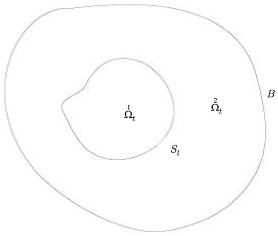
We consider a free boundary problem for a viscous compressible magnetohydrodynamics motion in domain ${\stackrel{1}{\mathrm{\Omega }}}_t$, bounded by a free surface $S_t.$ The motion interacts with an electromagnetic field located in ${\stackrel{2}{\mathrm{\Omega }}}_t$. Moreover, ${\stackrel{2}{\mathrm{\Omega }}}_t$ is bounded by a fixed boundary B. Hence, $\mathrm{\Omega }={\stackrel{1}{\mathrm{\Omega }}}_t\cup S_t\cup {\stackrel{2}{\mathrm{\Omega }}}_t$ and $\partial \mathrm{\Omega }=B$.

In Figure 1, we present the two-dimensional section of the considered problem.

Figure 1. Two-dimensional intersections of the considered problem.

In ${\stackrel{1}{\mathrm{\Omega }}}_t$, the magnetohydrodynamic motion of viscous compressible barotropic fluid is described by the following system of equations:

$$\begin{array}{cc}\hfill & {\rho }_{,t}+div(\rho v)=0\hfill \\ \hfill & \rho \left(v_{,t}+v·\nabla v\right)-div\mathbb{D}(v)+\nabla p(\rho )-{\mu }_1\stackrel{1}{H}·\nabla \stackrel{1}{H}+{\displaystyle \frac{1}{2}}{\mu }_1\nabla \stackrel{1}{H}{}^2=\rho f,\hfill \\ \hfill & {\mu }_1{\stackrel{1}{H}}_{,t}=-\mathrm{rot}\stackrel{1}{E},\hfill \\ \hfill & rot\stackrel{1}{H}={\sigma }_1(\stackrel{1}{E}+{\mu }_{1}v\times \stackrel{1}{H}),\hfill \\ \hfill & div\stackrel{1}{H}=0,\hfill \end{array}$$

(1)

where $v=v(x,t)=\left(v_1(x,t),v_2(x,t),v_3(x,t)\right)\in {\mathbb{R}}^3$ is the velocity of the fluid, $\rho =\rho (x,t)\in {\mathbb{R}}_{+}$ is the density, $\stackrel{1}{H}=\stackrel{1}{H}(x,t)=(\stackrel{1}{H}(x,t),{\stackrel{1}{H}}_2(x,t),{\stackrel{1}{H}}_3(x,t))\in {\mathbb{R}}^3$ is the magnetic field, $\stackrel{1}{E}=\stackrel{1}{E}(x,t)=({\stackrel{1}{E}}_1(x,t),{\stackrel{1}{E}}_2(x,t),{\stackrel{1}{E}}_3(x,t))\in {\mathbb{R}}^3$ is the electric field, $f=f(x,t)=\left(f_1(x,t),f_2(x,t),f_3(x,t)\right)\in {\mathbb{R}}^3$ is the external force field, and $x=\left(x_1,x_2,x_3\right)\in {\mathbb{R}}^3$ are Cartesian coordinates.

Since the fluid is considered barotropic, we have

$$p=p(\rho )$$

(2)

and $\mathbb{D}(v)={\left\{{\mathbb{D}}_{i,j}\right\}}_{i,j=1,2,3}$ is the strain tensor of the form

$${\mathbb{D}}_{ij}(\nu )=\mu \left({\displaystyle \frac{\partial v_i}{\partial x_j}}+{\displaystyle \frac{\partial v_j}{\partial x_i}}-{\displaystyle \frac{2}{3}}{\delta }_{ij}divv\right)+\nu {\delta }_{ij}divv,$$

(3)

where $\mu$ and $\nu$ are positive viscosity coefficients, and ${\delta }_{i,j}$ is the Kroneker delta, which is such that ${\delta }_{i,j}=1$ for $i=j$ and ${\delta }_{i,j}=0$ for $i\ne j$.

Moreover, ${\mu }_1$ is the constant magnetic permeability; ${\sigma }_1$ is the constant electric conductivity. For system (1), the following initial and boundary conditions are prescribed:

$${\displaystyle \begin{array}{cc}\hfill & \phantom{(}\overline{n}·\mathbb{D}(v)+\overline{n}p(\varrho )+{\mu }_1\overline{n}·\mathbb{T}=p_0\overline{n}\hfill \\ \hfill & {\rho |}_{t=0}{=\rho (0),v|}_{t=0}=v(0),\stackrel{1}{H}{|}_{t=0}=\stackrel{1}{H}(0),div\stackrel{1}{H}(0)=0\mathrm{in}\hspace{1em}{\mathrm{\Omega }}_0,\hfill \\ \hfill & {\stackrel{1}{\mathrm{\Omega }}}_t{{|}_{t=0}={\stackrel{1}{\mathrm{\Omega }}}_0,\hspace{1em}{S}_t|}_{t=0}=S_0,\hfill \end{array}}$$

(4)

where $\overline{n}$ is the unit vector outward to ${\stackrel{1}{\mathrm{\Omega }}}_t$ and normal to $S_t$ and $\mathbb{T}(\stackrel{1}{H})$ is the stress magnetic field tensor of the form

$$\mathbb{T}(\stackrel{1}{H})={\left\{{\stackrel{1}{H}}_i{\stackrel{1}{H}}_j-{\displaystyle \frac{1}{2}}{\stackrel{1}{H}}^2{\delta }_{ij}\right\}}_{i,j=1,2,3}.$$

(5)

The boundary condition (4)₁ implies the compatibility condition

$$\overline{n}(0)·\mathbb{D}(v(0))·\overline{\tau }(0)+{\mu }_1\overline{n}(0)·\stackrel{1}{H}(0)\overline{\tau }(0)·\stackrel{1}{H}(0)=0\mathrm{on}{S}_0,$$

(6)

where $\overline{n}(0)={\left.\overline{n}\right|}_{t=0},\overline{\tau }(0)={\left.\overline{\tau }\right|}_{t=0}$, and $\overline{\tau }$ is a tangent vector to $S_t$. In ${\stackrel{2}{\mathrm{\Omega }}}_t$, we have a motionless dielectric gas under the constant pressure $p_0$.

Therefore, we only have an electromagnetic field described by the system of equations

$$\begin{array}{cc}\hfill & {\mu }_2{\stackrel{2}{H}}_{,t}=-\mathrm{rot}\stackrel{2}{E},\hfill \\ \hfill & {\sigma }_2\stackrel{2}{E}=rot\stackrel{2}{H},\hfill \\ \hfill & div\stackrel{2}{H}=0,\hfill \end{array}$$

(7)

where ${\mu }_2$ is the constant magnetic permeability and ${\sigma }_2$ is the constant electric conductivity.

For system (7), the following initial and boundary conditions are prescribed:

$${\displaystyle \begin{array}{cc}\hfill & \phantom{(}\stackrel{2}{H}{|}_{t=0}=\stackrel{2}{H}(0),\hspace{1em}div\stackrel{2}{H}(0)=0,\hspace{1em}{\stackrel{2}{\mathrm{\Omega }}}_t{|}_{t=0}={\stackrel{2}{\mathrm{\Omega }}}_0,\hfill \\ \hfill & \stackrel{2}{H}·{\overline{\tau }}_{\alpha }{{|}_B=H_{\ast \alpha },\hspace{1em}\alpha =1,2,\hspace{1em}div\stackrel{2}{H}|}_B=0,\hfill \end{array}}$$

(8)

where ${\overline{\tau }}_{\alpha },\alpha =1,2$ are tangent vectors to B.

Problems (1)–(8) are composed of two problems. For a given $\stackrel{1}{H}$, we have the following problem for v and $\rho$:

$$\begin{array}{cccc}\hfill & {\rho }_t+div(\rho v)=0\hfill & \hfill & \mathrm{in}{\stackrel{1}{\mathrm{\Omega }}}_t,t\in (0,T),\hfill \\ \hfill & \rho \left(v_{,t}+v·\nabla v\right)-div\mathbb{D}(v)+\nabla p(\rho )\hfill \\ \hfill & ={\mu }_1\stackrel{1}{H}·\nabla \stackrel{1}{H}-{\displaystyle \frac{1}{2}}{\mu }_1\nabla \stackrel{1}{H}{}^2+\rho f\hfill & \hfill & \mathrm{in}{\stackrel{1}{\mathrm{\Omega }}}_t,t\in (0,T),\hfill \\ \hfill & {\left.\rho \right|}_{t=0}=\rho (0),{\left.v\right|}_{t=0}=v(0),{\stackrel{1}{\mathrm{\Omega }}}_t{|}_{t=0}={\stackrel{1}{\mathrm{\Omega }}}_0,\hfill \\ \hfill & \overline{n}·\mathbb{D}(v)+\overline{n}·\left(p(\rho )-p_0\right)=-{\mu }_1\overline{n}·\mathbb{T}(\stackrel{1}{H})\hfill & \hfill & \mathrm{on}{S}_t,t\in (0,T).\hfill \end{array}$$

(9)

Furthermore, for a given v, we have the following problem for $\stackrel{1}{H}$ and $\stackrel{2}{H}$:

$$\begin{array}{cccc}\hfill & {\mu }_1{\stackrel{1}{H}}_{,t}=-rot\stackrel{1}{E}\hfill & \hfill & \mathrm{in}{\stackrel{1}{\mathrm{\Omega }}}_t,\hfill \\ \hfill & rot\stackrel{1}{H}={\sigma }_1\left(\stackrel{1}{E}+{\mu }_{1}v\times \stackrel{1}{H}\right)\hfill & \hfill & \mathrm{in}{\stackrel{1}{\mathrm{\Omega }}}_t,\hfill \\ \hfill & div\stackrel{1}{H}=0\hfill & \hfill & \mathrm{in}{\stackrel{1}{\mathrm{\Omega }}}_t,\hfill \\ \hfill & {\mu }_2{\stackrel{2}{H}}_{,t}=-rot\stackrel{2}{E}\hfill & \hfill & \mathrm{in}{\stackrel{2}{\mathrm{\Omega }}}_t,\hfill \\ \hfill & rot\stackrel{2}{H}={\sigma }_2\stackrel{2}{E}\hfill & \hfill & \mathrm{in}{\stackrel{2}{\mathrm{\Omega }}}_t,\hfill \\ \hfill & div\stackrel{2}{H}=0\hfill & \hfill & \mathrm{in}{\stackrel{2}{\mathrm{\Omega }}}_t,\hfill \end{array}$$

(10)

where $t\in (0,T)$ and

$${\displaystyle \begin{array}{cc}\hfill & \phantom{(}\stackrel{1}{H}{|}_{t=0}=\stackrel{1}{H}(0),\hspace{1em}\hspace{1em}\hspace{1em}\hspace{1em}\stackrel{2}{H}{|}_{t=0}=\stackrel{2}{H}(0)\hfill \\ \hfill & \stackrel{2}{H}·{\overline{\tau }}_{\alpha }{{|}_B=H_{\ast \alpha },\hspace{1em}\alpha =1,2,div\stackrel{2}{H}|}_B=0.\hfill \end{array}}$$

Problem (10) is not complete because electromagnetic fields in ${\stackrel{1}{\mathrm{\Omega }}}_t$ and ${\stackrel{2}{\mathrm{\Omega }}}_t$ interact through the free surface $S_t$. The general transmission conditions are formulated in Lemma 1.1 in [1]. Recalling them, we have

$$\sum _{\alpha =1}^2\left(a_1\stackrel{1}{E}·{\overline{\tau }}_{\alpha }\overline{n}\times {\overline{\tau }}_{\alpha }·\stackrel{1}{H}-a_2\stackrel{2}{E}·{\overline{\tau }}_{\alpha }\overline{n}\times {\overline{\tau }}_{\alpha }·\stackrel{2}{H}\right)=0\mathrm{on}{S}_t,$$

(11)

where $a_1,a_2$ are arbitrary non-vanishing constants, $\overline{n}$ is the unit normal vector to $S_t$, and ${\overline{\tau }}_{\alpha },\alpha =1,2$ are tangent to $S_t$.

Eliminating the electric fields from (10), we obtain for any $t\in (0,T)$ the following problem:

$$\begin{array}{cc}{\mu }_1{\stackrel{1}{H}}_{,t}+\frac{1}{{\sigma }_1}{\mathrm{rot}}^2\stackrel{1}{H}={\mu }_1\mathrm{rot}(v\times \stackrel{1}{H})\hfill & \mathrm{in}\hspace{1em}{\stackrel{1}{\mathrm{\Omega }}}_t,\hfill \\ \hspace{0.17em}div\stackrel{1}{H}=0\hfill & \mathrm{in}\hspace{1em}{\stackrel{1}{\mathrm{\Omega }}}_t,\hfill \\ {\mu }_2{\stackrel{2}{H}}_{,t}+\frac{1}{{\sigma }_2}{\mathrm{rot}}^2\stackrel{2}{H}=0\hfill & \mathrm{in}\hspace{1em}{\stackrel{2}{\mathrm{\Omega }}}_t,\hfill \\ \hspace{0.17em}div\stackrel{2}{H}=0\hfill & \mathrm{in}\hspace{1em}{\stackrel{2}{\mathrm{\Omega }}}_t,\hfill \\ \hspace{0.17em}\stackrel{1}{H}{|}_{t=0}=\stackrel{1}{H}(0),\hspace{1em}div\stackrel{1}{H}(0)=0\hfill & \mathrm{in}\hspace{1em}{\stackrel{1}{\mathrm{\Omega }}}_0,\hfill \\ \hspace{0.17em}\stackrel{2}{H}{|}_{t=0}=\stackrel{2}{H}(0),\hspace{1em}div\stackrel{2}{H}(0)=0\hfill & \mathrm{in}\hspace{1em}{\stackrel{2}{\mathrm{\Omega }}}_0,\hfill \\ \hspace{0.17em}\stackrel{2}{H}·{\overline{\tau }}_{\alpha }^{\prime }=H_{\ast \alpha },\hspace{1em}\alpha =1,2,\hspace{1em}div\stackrel{2}{H}{|}_B=0\hfill & \mathrm{on}\hspace{1em}B,\hfill \end{array}$$

(12)

where ${\overline{\tau }}_{\alpha }^{\prime },\alpha =1,2$ are tangent vectors to B, and the transmission condition (11) takes the form

$$\begin{array}{cc}\hfill {\displaystyle \sum _{\alpha =1}^2}& \left[{\displaystyle \frac{a_1}{{\sigma }_1}}\left(\mathrm{rot}\stackrel{1}{H}-{\mu }_{1}v\times \stackrel{1}{H}\right)·{\overline{\tau }}_{\alpha }\overline{n}\times {\overline{\tau }}_{\alpha }·\stackrel{1}{H}\right.\hfill \\ \hfill & \left.-{\displaystyle \frac{a_2}{{\sigma }_2}}\mathrm{rot}\stackrel{2}{H}·{\overline{\tau }}_{\alpha }\overline{n}\times {\overline{\tau }}_{\alpha }·\stackrel{2}{H}\right]=0.\hfill \end{array}$$

(13)

In this paper, we prove the local existence of solutions to problems (10), (12), and (13). We prove it by the method of successive approximations described in problems (53) and (54).

The existence is proved in the Sobolev–Slobodetskii spaces defined in Section 2.1. We use the Besov-type spaces to describe more precisely the initial and boundary traces. Moreover, we are able to prove the local existence of solutions with sharp regularity with the lowest possible regularity that is necessary to handle the nonlinearity of the problem. To describe the main result precisely, we need to describe the following quantities:

We define Lagrangian coordinates in ${\stackrel{1}{\mathrm{\Omega }}}_t$ and ${\stackrel{2}{\mathrm{\Omega }}}_t$ as the initial data for the Cauchy problems (see (49)):

$${\displaystyle \frac{d\stackrel{i}{x}}{dt}}=\stackrel{i}{v}(\stackrel{i}{x},t),\stackrel{i}{x}{|}_{t=0}=\stackrel{i}{\xi }\in {\stackrel{i}{\mathrm{\Omega }}}_0,i=1,2.$$

(14)

Solving the equation, we get

$$\stackrel{i}{x}(\stackrel{i}{\xi },t)=\stackrel{i}{\xi }+\underset{0}{\overset{t}{\int }}\stackrel{i}{\overline{v}}(\stackrel{i}{\xi },\tau )d\tau ,$$

(15)

where $\stackrel{i}{\overline{v}}(\stackrel{i}{\xi },t)=\stackrel{i}{v}(\stackrel{i}{x}(\stackrel{i}{\xi },t),t),\stackrel{i}{\xi }\in {\stackrel{i}{\mathrm{\Omega }}}_0,i=1,2.$

However, to define the Lagrangian coordinate $\stackrel{2}{\xi }$, we need $\stackrel{2}{v}$ in ${\stackrel{2}{\mathrm{\Omega }}}_t$. Since we do not have it, we construct $\stackrel{2}{v}$ in ${\stackrel{2}{\mathrm{\Omega }}}_t$ as a solution to the problem (see (47))

$${\displaystyle \begin{array}{cc}\phantom{(}{\stackrel{2}{v}}_{,t}-div\mathbb{D}(\stackrel{2}{v})=0\hfill & \mathrm{in}\hspace{1em}{\stackrel{2}{\mathrm{\Omega }}}_t,\hfill \\ \stackrel{2}{v}{|}_{S-t}=\stackrel{1}{v}{|}_{S_t},\hspace{1em}\stackrel{2}{v}{|}_B=0,\hfill & \hfill \\ \stackrel{2}{v}{|}_{t=0}=\stackrel{2}{v}(0)\hfill & \mathrm{in}\hspace{1em}{\stackrel{2}{\mathrm{\Omega }}}_0.\hfill \end{array}}$$

(16)

Since $\stackrel{2}{v}$ is unknown, we construct it as a solution to the following elliptic problem (see (48)):

$$\begin{array}{c}div\mathbb{D}(\stackrel{2}{v}(0))=0\mathrm{in}{\stackrel{2}{\mathrm{\Omega }}}_0,\hfill \\ \stackrel{2}{v}(0){{|}_{S_0}=\stackrel{1}{v}(0)|}_{S_0}.\hfill \end{array}$$

(17)

Now, we formulate the main result.

Theorem 1.

Assume that $v(0)\in H^{1+\alpha }({\stackrel{1}{\mathrm{\Omega }}}_0)$, $\stackrel{1}{H}(0)\in H^{1+\alpha }({\stackrel{1}{\mathrm{\Omega }}}_0)$, $\stackrel{2}{H}(0)\in H^{1+\alpha }(\stackrel{2}{\mathrm{\Omega }}(0))$, ${\mathrm{\Omega }}_t{|}_{t=0}={\mathrm{\Omega }}_0$, $S_t{|}_{t=0}=S_0$, and $\alpha >3/4$. Assume that $\overline{f}\in H^{\alpha ,\alpha /2}(\stackrel{1 }{{\mathrm{\Omega }}_0^t})$ and $p=p(\varrho )$, where $p(\varrho )$ is a smooth function, $H_{\ast i}\in H^{3/2+\alpha ,3/4+\alpha /2}(B^t)$, $i=1,2$. Assume that $S_0\in H^{3/2+\alpha }$, and $x(\xi ,t)=\xi +{\int }_0^t\overline{v}(\xi ,t)d{t}^{\prime }$, $\overline{v}(\xi ,t)=v(x(\xi ,t),t)$, $\stackrel{1}{\overline{H}}(\xi ,t)=\stackrel{1}{H}(x(\xi ,t),t)$, and $\stackrel{2}{\overline{H}}(\xi ,t)=\stackrel{2}{H}(\stackrel{2}{x}(\xi ,t),\xi )$, where $\stackrel{2}{x}(\xi ,t)=\xi +{\int }_0^t\stackrel{2}{\overline{v}}(\xi ,t)$, $\stackrel{2}{\overline{v}}(\xi ,t)=\stackrel{2}{v}(x^2(\xi ,t),t)$, and $\stackrel{2}{v}$ is defined by (47).

Then, for sufficiently small t, there exists a local solution to problems (9), (12), and (13) such that $\overline{v}\in H^{2+\alpha ,1+\alpha /2}(\stackrel{1 }{{\mathrm{\Omega }}_0^t})$, $\stackrel{1}{H}\in H^{2+\alpha ,1+\alpha /2}(\stackrel{1 }{{\mathrm{\Omega }}_0^t})$, and $\stackrel{2}{\overline{H}}\in H^{2+\alpha ,1+\alpha /2}(\stackrel{2 }{{\mathrm{\Omega }}_0^t})$.

Now, we describe the proof of this theorem. Since the free boundary problem is considered, we need to use the Lagrangian coordinates.

In ${\stackrel{2}{\mathrm{\Omega }}}_t$, there is no velocity, so we introduce velocity $\stackrel{2}{v}$ in ${\stackrel{2}{\mathrm{\Omega }}}_t$ as a solution to problem (47).

Hence, we have $v=\stackrel{1}{v}$ in ${\stackrel{1}{\mathrm{\Omega }}}_t$ and $\stackrel{2}{v}$ in ${\stackrel{2}{\mathrm{\Omega }}}_t$. Hence, an evolution of the free surface $S_t$ and domains ${\stackrel{1}{\mathrm{\Omega }}}_t$, ${\stackrel{2}{\mathrm{\Omega }}}_t$ is described by the relation between Eulerian and Lagrangian coordinates.

The Lagrangian coordinates in ${\stackrel{1}{\mathrm{\Omega }}}_t$ and ${\stackrel{2}{\mathrm{\Omega }}}_t$ are introduced in (49) and (50).

Expressing problems (9) and (12) in the Lagrangian coordinates yields problems (51) and (52). To show the existence of solutions to problems (51) and (52), we construct a method of successive approximations described by problems (53) and (54).

Problem (53) is linear with respect to ${\overline{v}}_{n+1}$ and nonlinear in ${\overline{v}}_n$, $n\in N$. In Section 4, we derive the inequality

$$\parallel {\overline{v}}_{n+1}{\parallel }_{H^{2+\alpha ,1+\alpha /2}(\stackrel{1 }{{\mathrm{\Omega }}_0^t})}\le \varphi (t^a\parallel {\overline{v}}_n{\parallel }_{H^{2+\alpha ,1+\alpha /2}(\stackrel{1 }{{\mathrm{\Omega }}_0^t})},D_2),$$

(18)

where $a>0$,$D_2=\parallel v_0{\parallel }_{H^{1+\alpha }({\stackrel{1}{\mathrm{\Omega }}}_0)}+\parallel H_0{\parallel }_{H^{1+\alpha }({\stackrel{1}{\mathrm{\Omega }}}_0)}+\parallel {\rho }_0{\parallel }_{H^{1+\alpha }({\stackrel{1}{\mathrm{\Omega }}}_0)}+{\parallel \overline{f}\parallel }_{H^{\alpha ,\alpha /2}(\stackrel{1 }{{\mathrm{\Omega }}_0^t})}$, and $\varphi$ is an increasing positive function.

To derive estimate (18), we have to examine the operator

$${\overline{\rho }}_n({\overline{v}}_n){\overline{v}}_{n+1,t}-{div}_{\xi }{\mathbb{D}}_{\xi }({\overline{v}}_{n+1})=F,$$

(19)

where $\overline{F}$ and ${\overline{v}}_n$ are given and ${\overline{v}}_{n+1}$ is a solution. To obtain an estimate for the quantity

$$\parallel {\overline{v}}_{n+1}{\parallel }_{H^{2+\alpha ,1+\alpha /2}(\stackrel{1 }{{\mathrm{\Omega }}_0^t})}$$

(20)

we need the Hölder continuity of ${\overline{\rho }}_n({\overline{v}}_n)$ and appropriate partition of unity, which helps to derive an estimate for (20). This difficulty follows from the compressibility of the considered problem.

To formulate problem (52), we need Lagrangian coordinates in ${\stackrel{2}{\mathrm{\Omega }}}_0$, so we construct $\stackrel{2}{v}$ by problem (47). We describe the quantities (see expressions (14) to (17)) introduced prior in Theorem 1. Problem (54) is a linear problem for ${\stackrel{1}{\overline{H}}}_{n+1}$ and ${\stackrel{2}{\overline{H}}}_{n+1}$ and nonlinear with respect to ${\overline{v}}_n$ and ${\stackrel{1}{\overline{H}}}_n$, ${\stackrel{2}{\overline{H}}}_n$, with appropriate initial and boundary conditions and the transmission condition. It is a very complicated problem.

The existence and estimate for ${\stackrel{1}{\overline{H}}}_{n+1}$, ${\stackrel{2}{\overline{H}}}_{n+1}$ are derived by the regularizer technique. The method can be found in [2]. Estimates of nonlinear terms containing ${\stackrel{1}{\overline{H}}}_n$, ${\stackrel{2}{\overline{H}}}_n$, and ${\overline{v}}_n$ can be derived in the same way as in Section 4. Therefore, we have

$${\displaystyle \begin{array}{l}\phantom{(}{\displaystyle \sum _{i=1}^2}\parallel {\stackrel{i}{\overline{H}}}_{n+1}{\parallel }_{H^{2+\alpha ,1+\alpha /2}({\stackrel{i}{\mathrm{\Omega }}}_0^t)}\\ \le \varphi (t^a\parallel {\stackrel{1}{\overline{H}}}_n{\parallel }_{H^{2+\alpha ,1+\alpha /2}({\stackrel{1}{\mathrm{\Omega }}}_0^t)},t^a\parallel {\stackrel{2}{\overline{H}}}_n{\parallel }_{H^{2+\alpha ,1+\alpha /2}({\stackrel{1}{\mathrm{\Omega }}}_0^t)},\\ \parallel \stackrel{1}{H}{(0)\parallel }_{H^{1+\alpha }({\stackrel{1}{\mathrm{\Omega }}}_0)},\parallel \stackrel{2}{H}{(0)\parallel }_{H^{1+\alpha }({\stackrel{2}{\mathrm{\Omega }}}_0)},\parallel H_{\ast 1}{\parallel }_{H^{3/2+\alpha ,3/4+\alpha /2}(B^t)},\\ \parallel H_{\ast 2}{\parallel }_{H^{3/2+\alpha ,3/4+\alpha /2}(B^t)}),\end{array}}$$

(21)

where $a>0$.

From (18) and (21) and t being sufficiently small, we have

$$\parallel {\overline{v}}_n{\parallel }_{H^{2+\alpha ,1+\alpha /2}(\stackrel{1 }{{\mathrm{\Omega }}_0^t})}+\sum _{i=1}^2{\parallel \stackrel{i}{\overline{H}}\parallel }_{H^{2+\alpha ,1+\alpha /2}({\stackrel{i}{\mathrm{\Omega }}}_0^t)}\le \varphi (\mathrm{data}).$$

(22)

The above estimate and the standard estimates for differences imply the existence of the solutions described in Theorem 1.

The free boundary problems for incompressible and compressible magnetohydrodynamics were developed by P. Kacprzyk between 2003 and 2015 (see the references in [2]). The technique developed by P. Kacprzyk is based on the energy method. A more advanced technique developed in [1,2] for incompressible magnetohydrodynamics potentiates proving the existence of solutions with the lowest possible regularity for the considered nonlinear problem. The technique in this paper requires the results of V.A. Solonnikov (see the references in [2]). The mathematical motivation of the considered problem is that it is an open problem. Physically, it means that the magnetohydrodynamic fluid is kept in a bounded domain by the electromagnetic field. Hence, the fusion problem has a physical motivation.

2. Notation and Auxiliary Results

2.1. Spaces

We consider the anisotropic Sobolev–Slobodetskii spaces $H^{k+\alpha ,k/2+\alpha /2}({\mathrm{\Omega }}^T),\mathrm{\Omega }\subset {\mathbb{R}}^3,$ $k\in {\mathbb{N}}_0=\mathbb{N}\cup \left\{0\right\}$ and $\alpha \in (0,1)$ with the norm

$$\begin{array}{cc}\hfill {\parallel u\parallel }_{H^{k+\alpha ,k/2+\alpha /2}\left({\mathrm{\Omega }}^T\right)}^2& ={\displaystyle \sum _{|\beta |+2i⩽k}}{∥D_x^{\beta }{\partial }_t^{i}u∥}_{L_2\left({\mathrm{\Omega }}^T\right)}^2\hfill \\ \hfill & +{\displaystyle \sum _{|\beta |=k}}\underset{0}{\overset{T}{\int }}\underset{\mathrm{\Omega }}{\int }\underset{\mathrm{\Omega }}{\int }{\displaystyle \frac{{\left|D_{x^{\prime }}^{\beta }u(x^{\prime },t)-D_{x^{″}}^{\beta }u\left(x^{″},t\right)\right|}^2}{{\left|x^{\prime }-x^{″}\right|}^{3+2(k+\alpha -[k+\alpha ])}}}d{x}^{\prime }d{x}^{″}dt\hfill \\ \hfill & +\underset{\mathrm{\Omega }}{\int }\underset{0}{\overset{T}{\int }}\underset{0}{\overset{T}{\int }}{\displaystyle \frac{{\left|{\partial }_{t^{\prime }}^{[k/2+\alpha /2]}u\left(x,t^{\prime }\right)-{\partial }_{t^{″}}^{[k/2+\alpha /2]}u\left(x,t^{″}\right)\right|}^2}{{\left|t^{\prime }-t^{″}\right|}^{1+2\left(\frac{k}{2}+\frac{\alpha }{2}-\left[\frac{k}{2}+\frac{\alpha }{2}\right]\right)}}}d{t}^{\prime }d{t}^{″}dx,\hfill \end{array}$$

(23)

where $D_x^{\beta }={\partial }_{x_1}^{{\beta }_1}{\alpha }_{x_2}^{{\beta }_2}{\partial }_{x_3}^{{\beta }_3},|\beta |={\beta }_1+{\beta }_2+{\beta }_3,{\beta }_i\in N_0,i=1,2,3,\left[l\right]$ means the integer part of $l.$

In this paper, we need special spaces of (23) such that $k=2,\alpha \in (0,1)$. Hence, we use spaces $H^{2+2,1+\alpha /2}\left({\mathrm{\Omega }}^T\right)$ with the norm

$$\begin{array}{cc}\hfill {\parallel u\parallel }_{H^{2+\alpha ,1+\alpha /2}\left({\mathrm{\Omega }}^T\right)}^2& ={\displaystyle \sum _{|\beta |+2i⩽2}}{∥D_x^{\beta }{\partial }_t^{i}u∥}_{L_2\left({\mathrm{\Omega }}^T\right)}^2\hfill \\ \hfill & +{\displaystyle \sum _{|\beta |=2}}\underset{0}{\overset{T}{\int }}\underset{\mathrm{\Omega }}{\int }\underset{\mathrm{\Omega }}{\int }{\displaystyle \frac{{\left|D_{x^{\prime }}^{\beta }u(x^{\prime },t)-D_{x^{″}}^{\beta }u\left(x^{″},t\right)\right|}^2}{{\left|x^{\prime }-x^{″}\right|}^{3+2\alpha }}}d{x}^{\prime }d{x}^{″}dt\hfill \\ \hfill & +\underset{\mathrm{\Omega }}{\int }\underset{0}{\overset{T}{\int }}\underset{0}{\overset{T}{\int }}{\displaystyle \frac{{\left|{\partial }_{t^{\prime }}u\left(x,t^{\prime }\right)-{\partial }_{t^{″}}u\left(x,t^{″}\right)\right|}^2}{{\left|t^{\prime }-t^{″}\right|}^{1+\alpha }}}d{t}^{\prime }d{t}^{″}dx.\hfill \end{array}$$

(24)

In this paper, we also need the $L_p$-Besov spaces. Hence, we recall some properties of isotropic Besov spaces that are frequently used in this paper. Next, we define anisotropic Besov spaces and formulate some imbedding theorems that we need.

Let us introduce the differences

$${\mathrm{\Delta }}_i(h)u(x)=u\left(x+h{e}_i\right)-u(x),$$

where $x\in {\mathbb{R}}^n$ and $e_i,i=1,\dots ,n$ are the standard unit vectors. Then, we define the m-difference inductively as follows:

$${\mathrm{\Delta }}_i^m(h)u(x)={\mathrm{\Delta }}_i(h)\left({\mathrm{\Delta }}_i^{m-1}(h)u(x)\right)=\sum _{j=0}^m{(-1)}^m{c}_{jm}u\left(x+jh{e}_i\right),$$

where $c_{jm}=({\displaystyle \genfrac{}{}{0pt}{}{m}{j}})={\displaystyle \frac{m!}{j!(m-j)!}}$. Moreover, we introduce the difference

$$\mathrm{\Delta }(y)f(x)=f(x+y)-f(x),x,y\in {\mathbb{R}}^n$$

and inductively

$${\mathrm{\Delta }}^m(y)f(x)=\mathrm{\Delta }(y)\left({\mathrm{\Delta }}^{m-1}(y)f(x)\right).$$

Since

$$\mathrm{\Delta }(x-y)f(y)=f(x)-f(y)$$

we have

$${\mathrm{\Delta }}^m(x-y)f(y)=\sum _{i=1}^n{\mathrm{\Delta }}^m\left((x-y)e_i\right)f(y)=\sum _{i=1}^n{\mathrm{\Delta }}_i^m(h)f(y),$$

where the last equality holds for $(x-y)·e_i=h_i$.

We define the isotropic Besov spaces by describing their norm (see [3], Ch. 4, Sect. 18)

$${\parallel u\parallel }_{B_p^l\left({\mathbb{R}}^n\right)}={\parallel u\parallel }_{L_p\left({\mathbb{R}}^n\right)}+\sum _{i=1}^n{\left(\underset{0}{\overset{h_0}{\int }}dh\underset{{\mathbb{R}}^n}{\int }{\displaystyle \frac{{\left|{\mathrm{\Delta }}_i^m(h){\partial }_{x_i^k}^{k}u\right|}^p}{h^{1+(l-k)p}}}dx\right)}^{1/p},$$

(25)

where $m>l-k,m,k\in \mathbb{N}\cup \left\{0\right\},l\in {\mathbb{R}}_{+},l\ne \mathbb{Z},p\in (1,\infty )$.

It was shown in [4] that the Besov spaces defined by (25) all coincide and have equivalent norms for all $m,k$, satisfying $m>l-k.$

Next, we define the $L_p$-scale of Sobolev–Slobodetskii spaces by introducing the norm

$${\parallel u\parallel }_{W_p^l\left({\mathbb{R}}^n\right)}={\parallel u\parallel }_{L_p\left({\mathbb{R}}^n\right)}+\sum _{i=1}^n{\left({\int }_0^{h_0}dh\int {\displaystyle \frac{{\left|{\mathrm{\Delta }}_i(h){\partial }_{x_i}^{\left[l\right]}u\right|}^p}{h^{1+p(l-[l])}}}dx\right)}^{1/p},$$

(26)

where $l\notin \mathbb{Z},\left[l\right]$ is the integer part of l.

We frequently write $l=k+\alpha ,k\in \mathbb{N}\cup \left\{0\right\},\alpha \in (0,1)$, so $k=\left[l\right]$ and $\alpha =l-\left[l\right]$.

By the Golorkin theorem (see [4]), the norms of spaces $B_p^l\left({\mathbb{R}}^n\right)$ and $W_p^l\left({\mathbb{R}}^n\right)$ are equivalent.

We also define the norms

$${\parallel u\parallel }_{{\overline{B}}_p^l({\mathbb{R}}^n)}={\parallel u\parallel }_{L_p\left({\mathbb{R}}^n\right)}+\sum _{|\alpha |=k}{\left(\underset{{\mathbb{R}}^n}{\int }dx\underset{{\mathbb{R}}^n}{\int }dy{\displaystyle \frac{\mid {\mathrm{\Delta }}^m(x-y)D_y^{\alpha }{u(y)|}^p}{{|x-y|}^{n+p(l-k)}}}\right)}^{1/p}$$

(27)

for any $m>l-k$ and

$${\parallel u\parallel }_{{\overline{W}}_p^l}\left({\mathbb{R}}^n\right)={\parallel u\parallel }_{L_p({\mathbb{R}}^n)}+\sum _{|\alpha |=\left[l\right]}{\left(\underset{{\mathbb{R}}^n}{\int }dx\underset{{\mathbb{R}}^n}{\int }dy{\displaystyle \frac{\mid \mathrm{\Delta }(x-y)D_y^{\alpha }{u(y)|}^p}{{|x-y|}^{n+p(l-[l])}}}\right)}^{1/p}.$$

(28)

By [4], norms (27) and (28) are also equivalent. Moreover, norms (25)–(27) and (26)–(28) are equivalent too.

Now, we introduce the partial derivatives

$$\begin{array}{cc}& {⟨u⟩}_{\alpha ,x,p,{\mathrm{\Omega }}^t}={\left(\underset{0}{\overset{t}{\int }}d{t}^{\prime }\underset{\mathrm{\Omega }}{\int }\underset{\mathrm{\Omega }}{\int }{\displaystyle \frac{{\left|u\left(x^{\prime },t^{\prime }\right)-u\left(x^{″},t^{\prime }\right)\right|}^p}{{\left|x^{\prime }-x^{″}\right|}^{3+p\alpha }}}d{x}^{\prime }d{x}^{″}\right)}^{1/p},\hfill \\ & {⟨u⟩}_{{\displaystyle \frac{\alpha }{2}},t,p,{\mathrm{\Omega }}^t}={\left(\underset{\mathrm{\Omega }}{\int }dx\underset{0}{\overset{t}{\int }}\underset{0}{\overset{t}{\int }}{\displaystyle \frac{{\left|u\left(x,t^{\prime }\right)-u\left(x,t^{″}\right)\right|}^p}{{\left|t^{\prime }-t^{″}\right|}^{1+p\alpha /2}}}d{t}^{\prime }d{t}^{″}\right)}^{1/p},\hfill \end{array}$$

where $\mathrm{\Omega }\subset {\mathbb{R}}^3$. Let

$$L_p^k(\mathrm{\Omega })=\left\{u:\sum _{|\alpha |=k}{∥D_x^{\alpha }u∥}_{L_p(\mathrm{\Omega })}<\infty \right\}$$

We also need the following seminorms:

$${⟨u⟩}_{\alpha ,x,p,\mathrm{\Omega }}={\left(\underset{\mathrm{\Omega }}{\int }\underset{\mathrm{\Omega }}{\int }{\displaystyle \frac{{\left|u\left(x^{\prime }\right)-u\left(x^{″}\right)\right|}^p}{{\left|x^{\prime }-x^{″}\right|}^{3+p\alpha }}}d{x}^{\prime }d{x}^{″}\right)}^{1/p},$$

and

$$\begin{array}{cc}& {⟨u⟩}_{{\displaystyle \frac{\alpha }{2}},t,p,(0,t)}\hfill \end{array}={\left(\underset{0}{\overset{t}{\int }}\underset{0}{\overset{t}{\int }}{\displaystyle \frac{{\left|u\left(t^{\prime }\right)-u\left(t^{″}\right)\right|}^p}{{\left|t^{\prime }-t^{\prime }\right|}^{1+p\alpha /2}}}d{t}^{\prime }d{t}^{″}\right)}^{1/p},$$

where $\mathrm{\Omega }\subset {\mathbb{R}}^3$.

Lemma 1.

The following imbeddings

$${⟨D_x^{k}u⟩}_{\beta ,x,,p,\mathrm{\Omega }}⩽c{\parallel u\parallel }_{H^{l+\alpha }(\mathrm{\Omega })},\mathrm{\Omega }\subset {\mathbb{R}}^3,$$

(29)

where

$${\displaystyle \frac{3}{2}}-{\displaystyle \frac{3}{p}}+k+\beta \le l+\alpha ,\alpha ,\beta \in (0,1),p\in [1,\infty ],k,l\in \mathbb{N}\cup \left\{0\right\},$$

and

$${⟨{\partial }_t^{k}u⟩}_{{\displaystyle \frac{\beta }{2}},t,p,(0,t)}\le c\parallel u\parallel H^{1/2+\alpha /2}(0,t),$$

(30)

where ${\displaystyle \frac{1}{2}}-{\displaystyle \frac{1}{p}}+{\displaystyle \frac{\beta }{2}}+k⩽{\displaystyle \frac{1}{2}}+{\displaystyle \frac{\alpha }{2}}$

• and

$${\parallel u\parallel }_{L_p^k(\mathrm{\Omega })}⩽c{\parallel u\parallel }_{H^{l+\alpha }(\mathrm{\Omega })},\mathrm{\Omega }\subset {\mathbb{R}}^3,$$

(31)

where

$${\displaystyle \frac{3}{2}}-{\displaystyle \frac{3}{p}}+k\le l+\alpha ,$$

hold.

We recall the following imbedding theorems, which are frequently used in the paper:

Lemma 2.

• Let $l,l_1\in {\mathbb{R}}_{+},p,p_1\in (1,\infty ),p_1\ge p$. Let $\mathrm{\Omega }\subset {\mathbb{R}}^3$. If $3/p-3/p_1+l_1\le l$, then

  $$W_p^l(\mathrm{\Omega })\subset W_{p_1}^{l_1}(\mathrm{\Omega }).$$
• If ${\displaystyle \frac{3}{p}}-{\displaystyle \frac{3}{q}}+\alpha \le l,\alpha \in \mathbb{N}\cup \left\{0\right\},q\in [1,\infty ],q\ge p$, then

  $${\partial }_x^{\alpha }{W}_p^l(\mathrm{\Omega })\subset L_q(\mathrm{\Omega }).$$

Consider anisotropic Sobolev–Slobodetskii spaces $W_{p,q}^{l,l/2}(\mathrm{\Omega }\times (0,T))$ with the norm

$$\begin{array}{cc}& {\parallel u\parallel }_{W_{p,q}^{l,l/2}(\mathrm{\Omega }\times (0,T))}={\parallel u\parallel }_{L_{p,q}\left({\mathrm{\Omega }}^T\right)}+{⟨D_x^{\left[l\right]}u⟩}_{l-\left[l\right],x,p,q,{\mathrm{\Omega }}^T}\hfill \\ & +{⟨{\partial }_t^{\left[{\displaystyle \frac{l}{2}}\right]}u⟩}_{{\displaystyle \frac{l}{2}}-\left[{\displaystyle \frac{l}{2}}\right],t,p,q,{\mathrm{\Omega }}^T},\hfill \end{array}$$

where $\left[l\right]$ is the integer part of $l,p,q\in [1,\infty ]$,

$${⟨u⟩}_{\alpha ,x,p,q,{\mathrm{\Omega }}^T}={\left[\underset{0}{\overset{T}{\int }}dt{\left(\underset{\mathrm{\Omega }}{\int }\underset{\mathrm{\Omega }}{\int }{\displaystyle \frac{{\left|u\left(x^{\prime },t\right)-u\left(x^{″},t\right)\right|}^p}{{\left|x^{\prime }-x^{″}\right|}^{3+p\alpha }}}d{x}^{\prime }d{x}^{″}\right)}^{q/p}\right]}^{1/q},$$

where $\alpha \in (0,1)$ and

$${⟨u⟩}_{\alpha ,t,p,q,{\mathrm{\Omega }}^T}={\left[\underset{\mathrm{\Omega }}{\int }dx{\left(\underset{0}{\overset{T}{\int }}\underset{0}{\overset{T}{\int }}{\displaystyle \frac{{\left|u\left(x,t^{\prime }\right)-u\left(x,t^{″}\right)\right|}^q}{{\left|t^{\prime }-t^{″}\right|}^{1+q\alpha }}}d{t}^{\prime }d{t}^{″}\right)}^{p/q}\right]}^{1/p}.$$

Lemma 3.

Let $l,l^{\prime }\in {\mathbb{R}}_{+},p,q,p^{\prime },q^{\prime }\in [1,\infty ],p^{\prime }\ge p,q^{\prime }\ge q,\mathrm{\Omega }\subset {\mathbb{R}}^3$.

• Let

$${\displaystyle \frac{3}{p}}+{\displaystyle \frac{2}{q}}-{\displaystyle \frac{3}{p^{\prime }}}-{\displaystyle \frac{2}{q^{\prime }}}+l^{\prime }\le l.$$

Then, the imbedding

$$W_{p,q}^{l,l/2}(\mathrm{\Omega }\times (0,T))\subset W_{p^{\prime },q^{\prime }}^{l^{\prime },l^{\prime }/2}(\mathrm{\Omega }\times (0,T))$$

holds.

Now, we recall the trace theorems from [5].

Lemma 4

(Trace theorem). Let $S=\partial \mathrm{\Omega }$. Let $u\in W_{p,q}^{l,l/2}(\mathrm{\Omega }\times (0,T))$, $l\in {\mathbb{R}}_{+},(p,q)\in (1,\infty )$. Let $\phi ={\left.u\right|}_{S^T}$ be the trace of u on $S^T$. Then, $\phi \in W_{p,q}^{l-1/p,l/2-1/2q}(S\times (0,T))$ and

$${\parallel \phi \parallel }_{W_{p,q}^{l-1/p,l/2-1/2q}(S\times (0,T))}\le c{\parallel u\parallel }_{W_{p,q}^{l,l/2}(\mathrm{\Omega }\times (0,T)),}$$

where c does not depend on u.

Lemma 5

(Inverse trace theorem). Let $\phi \in W_{p,q}^{l-1/p,l/2-1/2q}(S\times (0,T))$, $l\in {\mathbb{R}}_{+},(p,q)\in (1,\infty )$. Then, there exists a function $u\in W_{p,q}^{l.l/2}(\mathrm{\Omega }\times (0,T))$ such that ${\left.u\right|}_{S^T}=\phi$, and there exists a constant c independent of φ such that

$${\parallel u\parallel }_{W_{p,q}^{l.l/2}(\mathrm{\Omega }\times (0,T))}\le c{\parallel \phi \parallel }_{W_{p,q}^{l-1/p,l/2-1/2q}(S\times (0,T))}.$$

Lemma 6

(Time trace theorem). Let $u\in W_{p,q}^{l,l/2}(\mathrm{\Omega }\times (0,T)),l\in {\mathbb{R}}_{+}$, $p,q\in (1,\infty ),t_0\in (0,T)$. Then, the time trace $\phi ={\left.u\right|}_{t=t_0}$ belongs to $W_p^{l-2/q}(\mathrm{\Omega })$, and there exists a constant c independent of u such that

$${\parallel \phi \parallel }_{W_p^{l-2/q}(\mathrm{\Omega })}⩽c{\parallel u\parallel }_{W_{p,q}^{l,l/2}(\mathrm{\Omega }\times (0,T)).}$$

Lemma 7

(Inverse time trace theorem). $Let\phi \in W_p^{l-2/q}(\mathrm{\Omega }),l\in {\mathbb{R}}_{+}$, $p,q\in (1,\infty )$. Then, there exists a function $u\in W_{p,q}^{l,l/2}(\mathrm{\Omega }\times (0,T))$ such that

$${\left.u\right|}_{t=t_0}=\phi ,t_0\in (0,T)$$

and

$${\parallel u\parallel }_{W_{p,q}^{l,l/2}(\mathrm{\Omega }\times (0,T))}\le c{\parallel \phi \parallel }_{W_p^{l-2/q}(\mathrm{\Omega })}.$$

Finally, we introduce the energy type space

$${\parallel u\parallel }_{V_2^{2+\alpha }\left({\mathrm{\Omega }}^t\right)}={\displaystyle \underset{t}{sup}}{\parallel u(t)\parallel }_{H^{1+\alpha }(\mathrm{\Omega })}+{\parallel u\parallel }_{H^{2+\alpha ,1+\alpha /2}\left({\mathrm{\Omega }}^t\right)}$$

2.2. Partition of Unity

2.2.1. The Partition of Unity for Linearized Problem (9)

To prove the existence of solutions, we need a partition of unity. We consider two collections of open subsets $\left\{{\omega }^{(k)}\right\}$ and $\left\{{\mathrm{\Omega }}^{(k)}\right\},k\in \mathfrak{M}\cup \mathfrak{N}$ such that ${\overline{\omega }}^{(k)}\subset {\mathrm{\Omega }}^{(k)}\subset {\mathrm{\Omega }}_0={\stackrel{1}{\mathrm{\Omega }}}_0\cup {\stackrel{2}{\mathrm{\Omega }}}_0,$${\bigcup }_k{\omega }^{(k)}={\bigcup }_k{\mathrm{\Omega }}^{(k)}={\mathrm{\Omega }}_0,$${\overline{\mathrm{\Omega }}}^{(k)}\cap S_0={\varphi }_0$, where ${\varphi }_0$ describes the empty set for $k\in$${\mathfrak{M}}_1\cup {\mathfrak{M}}_2,{\overline{\mathrm{\Omega }}}^{(k)}\cap S_0\ne {\varphi }_0$, where ${\varphi }_0$ describes the empty set for $k\in {\mathfrak{N}}_1$ and ${\overline{\mathrm{\Omega }}}^{(k)}\cap B\ne {\varphi }_0$, and where ${\varphi }_0$ describes the empty set for $k\in {\mathfrak{N}}_2,\mathfrak{N}={\mathfrak{N}}_1\cup {\mathfrak{N}}_2$. Moreover, subdomains with $k\in {\mathfrak{M}}_i$ are contained in $\stackrel{i}{{\mathrm{\Omega }}_0},i=1,2$.

We assume that at most $N_0$ of the ${\mathrm{\Omega }}^{(k)}$ sets have nonempty intersections, and that ${\displaystyle {sup}_k}diam{\mathrm{\Omega }}^{(k)}\le 2\lambda ,{\displaystyle {sup}_k}diam{\omega }^{(k)}\le \lambda$ for some $\lambda >0$. Let ${\zeta }^{(k)}(x)$ be a smooth function such that $0\le {\zeta }^{(k)}(x)\le 1,{\zeta }^{(k)}(x)=1$ for $x\in {\omega }^{(k)},{\zeta }^{(k)}(x)=0$ for $x\in {\mathrm{\Omega }}_0\setminus {\mathrm{\Omega }}^{(k)}$, and $\left|D_x^{\nu }{\zeta }^{(k)}(x)\right|\le c/{\lambda }^{|\nu |}$. Then, $1\le$${\sum }_k{\left({\zeta }^{(k)}(x)\right)}^2\le N_0$. Introducing the function

$${\eta }^{(k)}(x)={\displaystyle \frac{{\zeta }^{(k)}(x)}{{\sum }_l{\left({\zeta }^{(l)}(x)\right)}^2}}$$

we obtain that ${\eta }^{(k)}(x)=0$ for $x\in {\mathrm{\Omega }}_0\setminus {\mathrm{\Omega }}^{(k)},{\sum }_k{\eta }^{(k)}(x){\zeta }^{(k)}(x)=1$ and $\left|D_x^{\nu }{\eta }^{(k)}(x)\right|\le c/{\lambda }^{|\nu |}$.

We denote by ${\xi }^{(k)}$ an interior point of ${\omega }^{(k)}$ and ${\mathrm{\Omega }}^{(k)}$ for $k\in \mathfrak{M}$ and an interior point of ${\overline{\omega }}^{(k)}\cap S_0$ and of ${\overline{\mathrm{\Omega }}}^{(k)}\cap S_0$ for $k\in {\mathfrak{N}}_1$ and an interior point of ${\overline{\omega }}^{(k)}\cap B$ and of ${\overline{\mathrm{\Omega }}}^{(k)}\cap B$ for $k\in {\mathfrak{N}}_2$. For $k\in {\mathfrak{M}}_i,{\xi }^{(k)}\in {\mathrm{\Omega }}_0^i,i=1,2$. Let $x=\left(x_1,x_2,x_3\right)$ be the Cartesian system of coordinates with the origin located in the interior of ${\mathrm{\Omega }}_0$.

Then, by translations and rotations, we introduce a local coordinate system $y=\left(y_1,y_2,y_3\right)$ with the origin at ${\xi }^{(k)}\in {\mathrm{\Omega }}^{(k)}\cap S_0,k\in {\mathfrak{N}}_1$ such that the part ${\tilde{S}}_0^{(k)}=S_0\cap {\overline{\mathrm{\Omega }}}^{(k)}$ of the boundary $S_0$ is described by $y_3=F_k\left(y_1,y_2\right)$. We denote the transformation as $y=Y_k(x)$. Then, we introduce new coordinates defined by

$$z_i=y_i,i=1,2,z_3=y_3-F_k\left(y_1,y_2\right),k\in {\mathfrak{N}}_1.$$

We will denote this transformation by ${\widehat{\mathrm{\Omega }}}^{(k)}\ni z={\mathsf{\Phi }}_k(y)$, where $y\in {\mathrm{\Omega }}^{(k)}$.

We assume that the sets ${\widehat{\omega }}^{(k)},{\widehat{\mathrm{\Omega }}}^{(k)}$ are described in local coordinates at ${\xi }^{(k)}$ by the inequalities

$$\begin{array}{cc}& \left|y_i\right|<\lambda ,i=1,2,\left|y_3-F_k\left(y_1,y_2\right)\right|<\lambda ,\hfill \\ & \left|y_i\right|<2\lambda ,i=1,2,\left|y_3-F_k\left(y_1,y_2\right)\right|<2\lambda ,\hfill \end{array}$$

respectively. Moreover, $\left(y_1,y_2,y_3\right)\in {\stackrel{1}{\mathrm{\Omega }}}_0$ if $y_3>F_k\left(y_1,y_2\right)$ and $\left(y_1,y_2,y_3\right)\in$$\stackrel{2}{{\mathrm{\Omega }}_0}$ for $y_3<F_k\left(y_1,y_2\right)$. Let ${\mathsf{\Psi }}_k={\mathsf{\Phi }}_k\circ Y_k$. Then, $z={\mathsf{\Psi }}_k(x)$ and

$${\widehat{u}}^{(k)}(z,t)=u\left({\mathsf{\Psi }}_k^{-1}(z),t\right),{\tilde{u}}^{(k)}(z,t)={\widehat{u}}^{(k)}(z,t){\widehat{\zeta }}^{(k)}(z,t).$$

For $k\in \mathfrak{M}$, we have

$${\tilde{u}}^{(k)}(x,t)=u^{(k)}(x,t){\zeta }^{(k)}(x).$$

For $k\in {\mathfrak{N}}_2$, we introduce new local coordinates with origin at ${\xi }^{(k)}\in B\cap {\overline{\mathrm{\Omega }}}^{(k)}$ such that $y_3=F_k\left(y_1,y_2\right)$ locally describes $B\cap {\overline{\mathrm{\Omega }}}^{(k)}$. We also introduce the transformation $z_i=y_i,i=1,2,z_3=y_3-F_k\left(y_1,y_2\right)$ and assume that $z={\mathsf{\Phi }}_k(y)$ belongs to ${\widehat{\mathrm{\Omega }}}^{(k)}$ for $y\in {\mathrm{\Omega }}^{(k)}$.

Finally, ${\widehat{\omega }}^{(k)},{\widehat{\mathrm{\Omega }}}^{(k)}$ are described by the inequalities

$$\begin{array}{cc}& \left|y_i\right|<\lambda ,i=1,2,0<y_3-F_k\left(y_1,y_2\right)<\lambda ,\hfill \\ & \left|y_i\right|<2\lambda ,i=1,2,0<y_3-F_k\left(y_1,y_2\right)<2\lambda ,\hfill \end{array}$$

respectively.

Moreover, we introduce the notations r.h.s. (right-hand side) and l.h.s. (left-hand side).

By $\varphi$, we denote an increasing positive function such that $\varphi (0)\ne 0$, and it can change its form from formula to formula.

2.2.2. The Partition of Unity for the Linearized Problem (12)

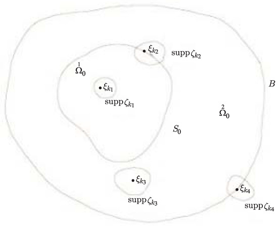
To apply the regularizer technique to the linearized problem (12), we need much more complicated partition of unity than in Section 2.2.1. The partition of unity contains four types of functions: ${\zeta }_1,{\zeta }_2,{\zeta }_3,{\zeta }_4.$ The supports of these functions and their interior points are presented in Figure 2, where $k_i\in {\mathbb{N}}_0,i=1,2,3,4$.

Figure 2. The partition of unity necessary for the proof of existence solution of magnetic field by the technique of regularizer.

The other properties of functions ${\zeta }_1,\dots ,{\zeta }_k$ are the same as in Section 2.2.1.

2.3. A Model Problem: Initial-Boundary Value Problem for a Parabolic System

We consider the following problem:

$$\begin{array}{cc}a{u}_t-{div}_x{\mathbb{D}}_x(u)=F(x,t)\hfill & \mathrm{in}{\mathrm{\Omega }}^T,\hfill \\ \overline{n}·{\mathbb{D}}_x(u)=G(x^{\prime },t)\hfill & \mathrm{on}{S}^T,\hfill \\ {\left.u\right|}_{t=0}=u(0)\hfill & \mathrm{in}\mathrm{\Omega },\hfill \end{array}$$

(32)

where $x^{\prime }\in S,a=a(x,t),a>0$ and either $\mathbb{D}$ is defined in (3) or ${div}_x{\mathbb{D}}_x$ is an elliptic operator.

Assumption 1.

$$\begin{array}{cc}& F(x,t)\in H^{\alpha ,\alpha /2}\left({\mathrm{\Omega }}^T\right),G\in H^{1/2+\alpha ,1/4+\alpha /2}\left(S^T\right),\hfill \\ & u(0)\in H^{1+\alpha }(\mathrm{\Omega }),\mathit{where}\alpha \in (0,1).\hfill \end{array}$$

Our aim is to prove the existence of solutions to (32) such that $u\in H^{2+\alpha ,1+\alpha /2}\left({\mathrm{\Omega }}^T\right)$. To show the existence of solutions to problem (32), we have to transform it to a problem with vanishing initial data.

Let $\tilde{u}$ be an extension of the initial data such that $\tilde{u}\in H^{2+{\alpha }_{1}1+\alpha /2}\left({\mathrm{\Omega }}^T\right)$ and ${\left.\tilde{u}\right|}_{t=0}=u(0)$. Introduce the function

$$w=u-\tilde{u}.$$

(33)

Then, w is a solution to the problem

$$\begin{array}{cc}\hfill & a{w}_t-{div}_x{\mathbb{D}}_x(w)=F(x,t)-a{\tilde{u}}_t+{div}_x{D}_x(\tilde{u})\equiv F^{\prime }(x,t),\hfill \\ \hfill & \overline{n}·D_x(w)=G(x^{\prime },t)-\overline{n}·D_x(\tilde{u})\equiv G^{\prime }(x,t),\hfill \\ \hfill & {\left.w\right|}_{t=0}=0.\hfill \end{array}$$

(34)

To prove the existence of solutions for problem (34), we use the regularizer technique (see [6], Ch. 4, Sect. 7). For this purpose, we have to consider problem (34) for all $t\in \mathbb{R}$.

First, we assume the compatibility conditions

$$\begin{array}{cc}\hfill & F(x,0)-\left({\left.a{\tilde{u}}_t\right|}_{t=0}-{div}_x{T}_x(u(0))\right)=0\mathrm{so}{\left.F^{\prime }\right|}_{t=0}=0,\hfill \\ \hfill & G(x^{\prime },0)-\overline{n}·\mathbb{D}\left({\left.u(0))\right|}_S=0\mathrm{so}{\left.G^{\prime }\right|}_{t=0}=0,\right.\hfill \end{array}$$

(35)

where the first condition yields

$${\tilde{u}}_t{|}_{t=0}={\displaystyle \frac{1}{{\left.a\right|}_{t=0}}}\left(F(x,0)+{div}_x{\mathbb{D}}_x(u(0))\right).$$

(36)

To examine problem (34) for $t\in \mathbb{R}$, we have to extend functions $F^{\prime }$ and $G^{\prime }$ for $t<0$ by zero. Therefore, we introduce

$$\begin{array}{c}\hfill {\tilde{F}}^{\prime }=\left\{\begin{array}{cc}{F}^{\prime }\hfill & \mathrm{for}t>0,\hfill \\ 0\hfill & \mathrm{for}t\le 0,\hfill \end{array}\right.\\ \\ \hfill {\tilde{G}}^{\prime }=\left\{\begin{array}{cc}{G}^{\prime }\hfill & \mathrm{for}t>0,\hfill \\ 0\hfill & \mathrm{for}t\le 0.\hfill \end{array}\right.\end{array}$$

(37)

and we need that ${\tilde{F}}^{\prime }\in H^{\alpha ,\alpha /2}(\mathrm{\Omega }\times R),{\tilde{G}}^{\prime }\in H^{1/2+\alpha ,1/4+\alpha /2}(S\times R)$, so we have

$${∥{\tilde{F}}^{\prime }∥}_{H^{\alpha ,\alpha /2}(\mathrm{\Omega }\times \mathbb{R})}\le c{∥F^{\prime }∥}_{\left.H^{\alpha ,\alpha /2}\left(\mathrm{\Omega }\times {\mathbb{R}}_{+}\right)\right)},$$

(38)

$${∥{\tilde{G}}^{\prime }∥}_{H^{1/2+\alpha ,1/4+\alpha /2}(S\times \mathbb{R})}\le c{∥G^{\prime }∥}_{H^{1/2+\alpha ,1/4+\alpha /2}\left(S\times {\mathbb{R}}_{+}\right)}.$$

(39)

To show (38), we have to examine the expression

$$\begin{array}{cc}& \underset{\mathrm{\Omega }}{\int }\underset{-\infty }{\overset{T}{\int }}\underset{-\infty }{\overset{T}{\int }}{\displaystyle \frac{{\left|{\tilde{F}}^{\prime }\left(x,t^{\prime }\right)-{\tilde{F}}^{\prime }\left(x,t^{″}\right)\right|}^2}{{\left|t^{\prime }-t^{″}\right|}^{1+\alpha }}}d{t}^{\prime }d{t}^{\prime }dx\hfill \\ \hfill =& \underset{\mathrm{\Omega }}{\int }dx\underset{-\infty }{\overset{0}{\int }}d{t}^{″}\underset{0}{\overset{T}{\int }}d{t}^{\prime }{\displaystyle \frac{{\left|{\tilde{F}}^{\prime }\left(x,t^{\prime }\right)\right|}^2}{{\left|t^{\prime }-t^{″}\right|}^{1+\alpha }}}+\underset{\mathrm{\Omega }}{\int }dx\underset{0}{\overset{T}{\int }}\underset{0}{\overset{T}{\int }}{\displaystyle \frac{{\left|F^{\prime }\left(x,t^{\prime }\right)-F^{\prime }\left(x,t^{″}\right)\right|}^2}{{\left|t^{\prime }-t^{″}\right|}^{1+\alpha }}}d{t}^{\prime }d{t}^{″},\hfill \end{array}$$

where the first term equals

$${\left.{\displaystyle \frac{1}{\alpha }}\underset{\mathrm{\Omega }}{\int }dx\underset{0}{\overset{T}{\int }}d{t}^{\prime }{\left|F^{\prime }\left(x,t^{\prime }\right)\right|}^2{\displaystyle \frac{1}{{\left|t^{\prime }-t^{″}\right|}^{\alpha }}}\right|}_{t^{″}=-\infty }^{t^{″}=0}={\displaystyle \frac{1}{\alpha }}\underset{\mathrm{\Omega }}{\int }dx\underset{0}{\overset{T}{\int }}d{t}^{\prime }{\displaystyle \frac{{\left|F^{\prime }\left(x,t^{\prime }\right)\right|}^2}{t^{\prime \alpha }}}$$

To show (38), we use Lemma 2 from [7], which implies

$$\underset{\mathrm{\Omega }}{\int }dx\underset{0}{\overset{T}{\int }}{\displaystyle \frac{{\left|F^{\prime }\left(x,t^{\prime }\right)\right|}^2}{t^{\prime \alpha }}}d{t}^{\prime }\le c\underset{\mathrm{\Omega }}{\int }dx\underset{0}{\overset{T}{\int }}\underset{0}{\overset{T}{\int }}{\displaystyle \frac{{\left|F^{\prime }\left(x,t^{\prime }\right)-F^{\prime }\left(x,t^{″}\right)\right|}^2}{{\left|t^{\prime }-t^{″}\right|}^{1+\alpha }}}d{t}^{\prime }d{t}^{″}$$

Hence, (38) is proved.

Next, we examine (39). Therefore, we calculate

$$\begin{array}{cc}& \underset{S}{\int }ds\underset{-\infty }{\overset{T}{\int }}\underset{-\infty }{\overset{T}{\int }}{\displaystyle \frac{{\left|{\tilde{G}}^{\prime }\left(s,t^{\prime }\right)-{\tilde{G}}^{\prime }\left(s,t^{″}\right)\right|}^2}{{\left|t^{\prime }-t^{″}\right|}^{1+2\left(\frac{1}{4}+\frac{\alpha }{2}-\left[\frac{1}{4}+\frac{\alpha }{2}\right]\right)}d{t}^{\prime }d{t}^{″}}}\hfill \\ \hfill =& \underset{S}{\int }ds\underset{-\infty }{\overset{0}{\int }}d{t}^{\prime }\underset{0}{\overset{T}{\int }}{\displaystyle \frac{{\left|G^{\prime }\left(s,t^{\prime }\right)\right|}^2}{{\left|t^{\prime }-t^{″}\right|}^{1+\frac{1}{2}+\alpha }}}d{t}^{\prime }+\underset{S}{\int }ds\underset{0}{\overset{T}{\int }}d{x}^{\prime }\underset{0}{\overset{T}{\int }}d{x}^{″}{\displaystyle \frac{{\left|G^{\prime }\left(s,t^{\prime }\right)-G^{\prime }\left(s,t^{″}\right)\right|}^2}{{\left|t^{\prime }-t^{″}\right|}^{1+1/2+\alpha }}}\hfill \end{array}$$

where the first equals

$${\displaystyle \frac{1}{\frac{1}{2}+\alpha }}\underset{S}{\int }ds\underset{0}{\overset{T}{\int }}{\displaystyle \frac{{\left|G^{\prime }\left(s,t^{\prime }\right)\right|}^2}{{\left|t^{\prime }\right|}^{1/2+\alpha }}}d{t}^{\prime }⩽c\underset{S}{\int }ds\underset{0}{\overset{T}{\int }}\underset{0}{\overset{T}{\int }}{\displaystyle \frac{{\left|G^{\prime }\left(s,t^{\prime }\right)-G^{\prime }\left(s,t^{″}\right)\right|}^2}{{\left|t^{\prime }-t^{″}\right|}^{1+1/2+\alpha }}}d{t}^{\prime }d{t}^{″},$$

and where the second inequality follows from Lemma 2 from [7]. Hence, (39) is proved.

In view of the above considerations, problem (34) takes the form

$$\begin{array}{cc}a{\tilde{w}}_t-{div}_x{\mathbb{D}}_x\tilde{w}={\tilde{F}}^{\prime }\hfill & \mathrm{in}\mathrm{\Omega }\times (-\infty ,T),\hfill \\ \overline{n}·{\mathbb{D}}_x(\tilde{w})={\tilde{G}}^{\prime }\hfill & \mathrm{in}S\times (-\infty ,T),\hfill \end{array}$$

(40)

where

$$\tilde{w}=\left\{\begin{array}{cc}w\hfill & \mathrm{for}t>0,\hfill \\ 0\hfill & \mathrm{for}t\le 0,\hfill \end{array}\right.$$

Applying the regularizer technique described in [6] (Ch. 4, Sect. 7) and the partition of unity from Section 2.2.1, we have

Lemma 8.

Assume that $a\in C^{\alpha ,\alpha /2}\left(\mathrm{\Omega }\times {\mathbb{R}}^T\right),\alpha \in (0,1),a\ge a_{\ast }$, where $a_{\ast }$ is a positive constant.

Assume that ${\tilde{F}}^{\prime }\in H^{\alpha ,\alpha /2}\left(\mathrm{\Omega }\times {\mathbb{R}}^T\right),{\tilde{G}}^{\prime }\in H^{1/2+\alpha ,1/4+\alpha /2}\left(S\times {\mathbb{R}}^T\right).$

Then, there exists a solution to (40) such that $\tilde{w}\in H^{2+\alpha ,1+\alpha /2}\left(\mathrm{\Omega }\times {\mathbb{R}}^T\right)$, and the following estimate holds

$$\begin{array}{c}\parallel \tilde{w}{\parallel }_{H^{2+\alpha ,1+\alpha /2}\left(\mathrm{\Omega }\times {\mathbb{R}}^T\right)}⩽c\left({∥{\tilde{F}}^{\prime }∥}_{H^{\alpha ,\alpha /2}\left(\mathrm{\Omega }\times {\mathbb{R}}^T\right)}+{∥{\tilde{G}}^{\prime }∥}_{H^{1/2+\alpha ,1/4+\alpha /2}\left(S\times {\mathbb{R}}^T\right)}\right),\end{array}$$

(41)

where ${\mathbb{R}}^T=(-\infty ,T)$.

In view of Lemma 8 and Lemma 2 from [7] and (33), we get

Lemma 9.

Assume that $a\in C^{\alpha ,\alpha /2}\left({\mathrm{\Omega }}^T\right),\alpha \in (0,1),a⩾a_{\ast }$, where $a_{\ast }$ is a positive constant. Assume that $F\in H^{\alpha ,\alpha /2}\left({\mathrm{\Omega }}^T\right),G\in H^{1/2+\alpha ,1/4+\alpha /2}\left(S^T\right)$, $u(0)\in H^{1+\alpha }(\mathrm{\Omega })$. Then, there exists a solution to problem (32) such that $u\in H^{2+\alpha ,1+\alpha /2}(\mathrm{\Omega })$ and

$$\begin{array}{cc}\hfill & {\parallel u\parallel }_{H^{2+\alpha ,1+\alpha /2}\left({\mathrm{\Omega }}^T\right)}⩽c\left({\parallel F\parallel }_{H^{\alpha ,\alpha /2}\left({\mathrm{\Omega }}^T\right)}\right.\hfill \\ \hfill & \left.+{\parallel G\parallel }_{H^{1/2+\alpha ,1/4+\alpha /2}\left(S^T\right)}+{\parallel u(0)\parallel }_{H^{1+\alpha }(\mathrm{\Omega })}\right).\hfill \end{array}$$

(42)

The linearized problem (12) has the form

$$\begin{array}{cccc}\hfill & {\mu }_1{\stackrel{1}{H}}_{,t}+{\displaystyle \frac{1}{{\sigma }_1}}{rot}_x^2\stackrel{1}{H}=M_1\hfill & \hfill & \mathrm{in}{\stackrel{1}{\mathrm{\Omega }}}_0^T,\hfill \\ \hfill & {div}_x\stackrel{1}{H}=N_1\hfill & \hfill & \mathrm{in}{\stackrel{1}{\mathrm{\Omega }}}_0^T,\hfill \\ \hfill & {\mu }_2{\stackrel{2}{H}}_{,t}+{\displaystyle \frac{1}{{\sigma }_2}}{rot}_x^2\stackrel{2}{H}=M_2\hfill & \hfill & \mathrm{in}{\stackrel{2}{\mathrm{\Omega }}}_0^T,\hfill \\ \hfill & {div}_x\stackrel{2}{H}=N_2\hfill & \hfill & \mathrm{in}{\stackrel{2}{\mathrm{\Omega }}}_0^T,\hfill \\ \hfill & \left({\displaystyle \frac{1}{{\sigma }_1}}{rot}_x\stackrel{1}{H}-{\displaystyle \frac{1}{{\sigma }_2}}{rot}_x\stackrel{2}{H}\right)·{\overline{\tau }}_{\alpha }=K_{\alpha },\alpha =1,2,\hfill & \hfill & \mathrm{on}{S}_0^T,\hfill \\ \hfill & (\stackrel{1}{H}-\stackrel{2}{H})·\overline{n}\times {\overline{\tau }}_{\alpha }=L_{\alpha },\alpha =1,2,\hfill & \hfill & \mathrm{on}{S}_0^T,\hfill \\ \hfill & {\left.\stackrel{2}{H}·{\overline{\tau }}_{\alpha }\right|}_B=H_{\ast \alpha },\alpha =1,2,{div}_x\stackrel{2}{H}{|}_B=D\hfill & \hfill & \mathrm{on}{B}^T,\hfill \\ \hfill & \stackrel{i}{H}{|}_{t=0}=\stackrel{i}{H}(0),\hfill \end{array}$$

(43)

where $M_i\in H^{\alpha ,\alpha /2}(\stackrel{i }{{\mathrm{\Omega }}_0^T}),N_i\in H^{1+\alpha ,1/2+\alpha /2}(\stackrel{i }{{\mathrm{\Omega }}_0^T}),i=1,2$,

$$\begin{array}{cc}\hfill & K_{\alpha }\in H^{1/2+\alpha ,1/4+\alpha /2}\left(S_0^T\right),L_{\alpha }\in H^{{\displaystyle \frac{3}{2}}+\alpha ,{\displaystyle \frac{3}{4}}+\alpha /2}\left(S_0^T\right),\alpha =1,2\hfill \\ \hfill & H_{\ast \alpha }\in H^{3/2+\alpha ,3/4+\alpha /2}\left(B^T\right),\alpha =1,2,D\in H^{1/2+\alpha ,1/4+\alpha /2}\left(B^T\right),\hfill \\ \hfill & \stackrel{i}{H}(0)\in H^{1+\alpha }({\stackrel{i}{\mathrm{\Omega }}}_0),i=1,2.\hfill \end{array}$$

(44)

Repeating the considerations leading to Lemma 9 and using the partition of unity introduced in Figure 1 and also applying the regularizer technique, we get

Lemma 10.

Let assumptions (44) hold. Then, there exists a solution to problem (43) such that $\stackrel{i}{H}\in H^{2+\alpha ,1+\alpha /2}(\stackrel{i }{{\mathrm{\Omega }}_0^T}),i=1,2$, and

$$\begin{array}{cc}\hfill {\displaystyle \sum _{i=1}^2}& \parallel \stackrel{i}{H}{\parallel }_{H^{2+\alpha ,1+\alpha /2}(\stackrel{i }{{\mathrm{\Omega }}_0^T})}\hfill \\ \hfill & \le c{\displaystyle \sum _{i=1}^2}\left({∥M_i∥}_{H^{\alpha ,\alpha /2}(\stackrel{i }{{\mathrm{\Omega }}_0^T})}+{∥N_i∥}_{H^{1+\alpha ,1/2+\alpha /2}(\stackrel{i }{{\mathrm{\Omega }}_0^T})}\right.\hfill \\ \hfill & +{∥K_i∥}_{H^{1/2+\alpha ,1/4+\alpha /2}\left(S_0^T\right)}+{∥L_i∥}_{H^{3+\alpha ,{\displaystyle \frac{3}{4}}+\alpha /2}\left(S_0^T\right)}\hfill \\ \hfill & \left.+{∥H_{\ast i}∥}_{H^{3/2+\alpha ,3/4}+\alpha /2\left(B^T\right)}+{\parallel \stackrel{i}{H}(0)\parallel }_{H^{1+\alpha }(\stackrel{i }{{\mathrm{\Omega }}_0^T})}\right)\hfill \\ \hfill & +{c\parallel D\parallel }_{H^{1/2+\alpha ,1/4+\alpha /2}\left(B^T\right)}.\hfill \end{array}$$

(45)

2.4. Notation

We use the following simplified notation: $\varphi$ always denotes an increasing positive function

$$\begin{array}{cc}{\delta }_{1n}(t)=t^a{∥{\overline{v}}_n∥}_{H^{2+\alpha ,,1+\alpha /2}(\stackrel{1 }{{\mathrm{\Omega }}_0^t})},\hfill & a>0,\hfill \\ {\delta }_{2n}(t)=t^a{\parallel \stackrel{1}{{\overline{H}}_n}\parallel }_{H^{2+\alpha ,1+\alpha /2}(\stackrel{1 }{{\mathrm{\Omega }}_0^t}),}\hfill \\ {\delta }_{3n}(t)=t^a{\parallel {\stackrel{2}{\overline{H}}}_n\parallel }_{H^{2+\alpha ;1+\alpha /2}(\stackrel{2 }{{\mathrm{\Omega }}_0^t})},\hfill \end{array}$$

where $\overline{u}(\xi ,t)=u(x(\xi ,t),t),x(\xi ,t)=\xi +{\int }_0^t\overline{v}(\xi ,t^{\prime })d{t}^{\prime }$, and $x=x(\xi ,t)$ describes the relation between Lagrangian and Eulerian coordinates.

3. Method of Successive Approximations

Let $v=v(x,t),x\in {\stackrel{1}{\mathrm{\Omega }}}_t$ be given.

Definition 1.

The Lagrangian coordinates in ${\stackrel{1}{\mathrm{\Omega }}}_0$ are initial data to the Cauchy problem

$${\displaystyle \frac{dx}{dt}}=v(x,t),{\left.x\right|}_{t=0}=\xi \in {\stackrel{1}{\mathrm{\Omega }}}_0$$

(46)

Hence, the domain ${\stackrel{1}{\mathrm{\Omega }}}_t$ is defined by

$${\stackrel{1}{\mathrm{\Omega }}}_t=\left\{x\in {\mathbb{R}}^3:x=x(\xi ,t)=\xi +{\int }_0^t\overline{v}\left(\xi ,t^{\prime }\right)d{t}^{\prime },\xi \in {\overline{\mathrm{\Omega }}}_0^1\right\},$$

where $\overline{v}(\xi ,t)=v(x(\xi ,t),t)$.

In free boundary problems in hydrodynamics, the free boundary at any time $t>0$ is built up from the same fluid particles as at time $t=0$ because ${\left.v\right|}_{S_t}$ is tangent to $S_t$.

To formulate problem (12) in Lagrangian coordinates, we have to introduce them in $\stackrel{2}{\mathrm{\Omega }}$ artificially because there is no velocity in ${\stackrel{2}{\mathrm{\Omega }}}_t$. For this purpose, we need

Definition 2.

Let $\stackrel{1}{v}=v$ be defined in ${\stackrel{1}{\mathrm{\Omega }}}_t$. Then, we construct $\stackrel{2}{v}$ in ${\stackrel{2}{\mathrm{\Omega }}}_t$ as a solution to the parabolic problem

$${\displaystyle \begin{array}{l}\phantom{(}{\stackrel{2}{v}}_{,t}-div\mathbb{D}(\stackrel{2}{v})=0\mathrm{in}{\stackrel{2}{\mathrm{\Omega }}}_t,\\ \stackrel{2}{v}{|}_{S_t}=\stackrel{1}{v}{|}_{S_t},\stackrel{2}{v}{|}_B=0,\\ \stackrel{2}{v}{|}_{t=0}=\stackrel{2}{v}(0)\hspace{1em}\hspace{1em}\hspace{1em}\mathrm{in}{\stackrel{2}{\mathrm{\Omega }}}_0.\end{array}}$$

(47)

Since $\stackrel{2}{v}(0)$ is unknown, we construct it as a solution to the following elliptic problem

$${\displaystyle \begin{array}{l}\phantom{(}div\mathbb{D}(\stackrel{2}{v}(0))=0\mathrm{in}\hspace{1em}{\stackrel{2}{\mathrm{\Omega }}}_0,\\ \stackrel{2}{v}{(0)|}_{S_0}=\stackrel{1}{v}(0){{|}_{S_0}\hspace{1em}\stackrel{2}{v}(0)|}_B=0\end{array}}$$

(48)

A proof of the existence of solutions to (47) is similar to the proof from [8], where parabolic system (47) with the slip boundary conditions was considered. Having $\stackrel{2}{v}$ constructed by problems (47) and (48), we can introduce Lagrangian coordinates $\stackrel{1}{\xi },\stackrel{2}{\xi }$ as the Cauchy data to the problems

$${\displaystyle \frac{d\stackrel{i}{x}}{dt}}=\stackrel{i}{v}(\stackrel{i}{x},t),\stackrel{i}{x}{|}_{t=0}=\stackrel{i}{\xi }\in {\stackrel{i}{\mathrm{\Omega }}}_0,i=1,2.$$

(49)

Then,

$$\begin{array}{cc}\hfill {\stackrel{i}{\mathrm{\Omega }}}_t=& \{\stackrel{i}{x}\in {\mathbb{R}}^3:\stackrel{i}{x}=\stackrel{i}{x}(\stackrel{i}{\xi },t)=\stackrel{i}{\xi }+\underset{0}{\overset{t}{\int }}\stackrel{i}{v}(\stackrel{i}{x}(\stackrel{i}{\xi },t^{\prime }),t^{\prime })d{t}^{\prime }\hfill \\ \hfill & =\stackrel{i}{\xi }+\underset{0}{\overset{t}{\int }}\stackrel{i}{\overline{v}}(\stackrel{i}{\xi },t^{\prime })d{t}^{\prime },\stackrel{i}{\xi }\in {\stackrel{i}{\mathrm{\Omega }}}_0\},i=1,2,\hfill \end{array}$$

(50)

where $\stackrel{i}{\overline{v}}(\stackrel{i}{\xi },t)=\stackrel{i}{v}(\stackrel{i}{x}(\stackrel{i}{\xi },t),t),\stackrel{i}{\xi }\in {\stackrel{i}{\mathrm{\Omega }}}_0,i=1,2.$

Expressing problems (9) and (12) in Lagrangian coordinates yields

$$\begin{array}{cc}\hfill & {\displaystyle \frac{d}{dt}}\overline{\rho }(\xi ,t)=-{div}_{\overline{v}}\overline{v}\overline{\rho }(\xi ,t),\hfill \\ \hfill & \overline{\rho }{\overline{v}}_{,t}-{div}_{\overline{v}}{\mathbb{D}}_{\overline{v}}(\overline{v})=\overline{\rho }\overline{f}-{\nabla }_{\overline{v}}p(\overline{\rho })+{\mu }_1{div}_{\overline{v}}\mathbb{T}(\stackrel{1}{\overline{H}}),\hfill \\ \hfill & {\overline{n}}_{\overline{v}}·{\mathbb{D}}_{\overline{v}}(\overline{v})=-{\overline{n}}_{\overline{v}}\left(p(\overline{\rho })-p_0\right)-{\mu }_1{\overline{n}}_{\overline{v}}\mathbb{T}(\stackrel{1}{\overline{H}}),\hfill \\ \hfill & {\left.\overline{\rho }\right|}_{t=0}=\rho (0),{\left.\overline{v}\right|}_{t=0}=v(0)\hfill \end{array}$$

(51)

and

$$\begin{array}{cccc}\hfill & {\mu }_1{\stackrel{1}{\overline{H}}}_{,t}+{\displaystyle \frac{1}{{\sigma }_1}}{rot}_{\stackrel{1}{\overline{v}}}^2\stackrel{1}{\overline{H}}={\mu }_1{rot}_{\stackrel{1}{\overline{v}}}\left(\stackrel{1}{\overline{v}}\times \stackrel{1}{\overline{H}}\right)+{\mu }_1\stackrel{1}{\overline{v}}·{\nabla }_{\stackrel{1}{\overline{v}}}\stackrel{1}{\overline{H}}\hfill & \hfill & \mathrm{in}{\stackrel{1}{\mathrm{\Omega }}}_0^T,\hfill \\ \hfill & {div}_{\stackrel{1}{\overline{v}}}\stackrel{1}{\overline{H}}=0\hfill & \hfill & \mathrm{in}{\stackrel{1}{\mathrm{\Omega }}}_0^T,\hfill \\ \hfill & {\mu }_2{\stackrel{2}{\overline{H}}}_{,t}+{\displaystyle \frac{1}{{\sigma }_2}}{rot}_{\stackrel{2}{\overline{v}}}^2\stackrel{2}{\overline{H}}={\mu }_2\stackrel{2}{\overline{v}}·{\nabla }_{\stackrel{2}{\overline{v}}}\stackrel{2}{\overline{H}}\hfill & \hfill & \mathrm{in}{\stackrel{2}{\mathrm{\Omega }}}_0^T,\hfill \\ \hfill & {div}_{\stackrel{2}{\overline{v}}}\stackrel{2}{\overline{H}}=0\hfill & \hfill & \mathrm{in}{\stackrel{2}{\mathrm{\Omega }}}_0^T,\hfill \\ \hfill & \left({\displaystyle \frac{1}{{\sigma }_1}}{\mathrm{rot}}_{\stackrel{1}{\overline{v}}}\stackrel{1}{\overline{H}}-{\displaystyle \frac{1}{{\sigma }_2}}{\mathrm{rot}}_{\stackrel{2}{\overline{v}}}\stackrel{1}{\overline{H}}\right)·{\overline{\tau }}_{\overline{v}\alpha }={\mu }_1\overline{v}\times \stackrel{1}{\overline{H}}·{\overline{\tau }}_{\overline{v}\alpha },\alpha =1,2,\hfill & \hfill & \mathrm{on}{S}_0^T,\hfill \\ \hfill & (\stackrel{1}{\overline{H}}-\stackrel{2}{\overline{H}})·({\overline{n}}_{\overline{v}}\times {\overline{\tau }}_{\overline{v}\alpha })=0,\alpha =1,2,\hfill & \hfill & \mathrm{on}{S}_0^T,\hfill \\ \hfill & \stackrel{2}{\overline{H}}·{\overline{\tau }}_{\alpha }{{|}_{t=0}=H_{\ast \alpha },\alpha =1,2,{div}_{\stackrel{2}{\overline{v}}}\stackrel{2}{\overline{H}}|}_B=0\hfill & \hfill & \mathrm{on}{B}^T,\hfill \\ \hfill & \stackrel{i}{\overline{H}}{|}_{t=0}=\stackrel{i}{H}(0)\hfill & \hfill & \mathrm{in}{\stackrel{i}{\mathrm{\Omega }}}_0,i=1,2,\hfill \end{array}$$

(52)

where $\overline{v}=\stackrel{1}{\overline{v}}$ in ${\stackrel{1}{\mathrm{\Omega }}}_t,\overline{v}=\stackrel{1}{\overline{v}}=\stackrel{2}{\overline{v}}$ in $S_0$, and ${\nabla }_{\overline{v}}={\left.{\displaystyle \frac{\partial {\xi }_k}{\partial x}}\right|}_{x=x(\xi ,t)}{\partial }_{{\xi }_k},x(\xi ,t)=\xi +\underset{0}{\overset{t}{\int }}\overline{v}\left(\xi ,t^{\prime }\right)d{t}^{\prime }$.

Moreover, any operator with subscript $\overline{v}$ means that it contains the transformed gradient ${\nabla }_{\overline{v}}$, and any operator with subscript ξ contains derivatives with respect to ξ.

To prove the existence of local solutions to problems (51) and (52), we apply the following method of successive approximations. Let ${\overline{v}}_n={\stackrel{1}{\overline{v}}}_n,{\stackrel{2}{\overline{v}}}_n$ be given. Then,

$${\displaystyle \begin{array}{ll}\phantom{(}\frac{d}{dt}{\overline{\varrho }}_n=-{div}_{{\overline{v}}_n}{\overline{v}}_n{\overline{\varrho }}_n,& \\ {\overline{\varrho }}_n{\overline{v}}_{n+1,t}-{div}_{\xi }{\mathbb{D}}_{\xi }({\overline{v}}_{n+1})& \\ =-(div{\mathbb{D}}_{\xi }({\overline{v}}_n)-div{\overline{v}}_n{\mathbb{D}}_{{\overline{v}}_n}({\overline{v}}_n))-{\nabla }_{{\overline{v}}_n}p({\overline{\varrho }}_n)+{\mu }_1{div}_{{\overline{v}}_n}\mathbb{T}({\stackrel{1}{\overline{H}}}_n)+{\overline{\varrho }}_n\overline{f}& \\ \equiv {\overline{F}}_n& \mathrm{in}\hspace{1em}\stackrel{1 }{{\overline{\mathrm{\Omega }}}_0^T},\\ {\overline{n}}_{\xi }·{\mathbb{D}}_{\xi }({\overline{v}}_{n+1})& \\ ={\overline{n}}_{\xi }·{\mathbb{D}}_{\xi }({\overline{v}}_n)-{\overline{n}}_{{\overline{v}}_n}·{\mathbb{D}}_{{\overline{v}}_n}({\overline{v}}_n)-{\overline{m}}_{{\overline{v}}_n}(p({\overline{\varrho }}_n)-p_0)-{\mu }_1{\overline{n}}_{{\overline{v}}_n}\mathbb{T}({\stackrel{1}{\overline{H}}}_n)\equiv {\overline{G}}_n& \mathrm{on}\hspace{1em}{S}_0^T\\ {\overline{v}}_{n+1}{{|}_{t=0}=v(0),\hspace{1em}{\overline{\varrho }}_n|}_{t=0}=\varrho (0)& \mathrm{in}\hspace{1em}{\stackrel{1}{\mathrm{\Omega }}}_0,\end{array}}$$

(53)

where ${\overline{v}}_n={\stackrel{1}{\overline{v}}}_n$. Let ${\stackrel{i}{\overline{H}}}_n,i=1,2$, be given.

Then, ${\stackrel{i}{\overline{H}}}_{n+1},i=1,2$ are solutions to the problem

$$\begin{array}{cccc}\hfill & {\mu }_1{\stackrel{1}{\overline{H}}}_{n+1,t}+{\displaystyle \frac{1}{{\sigma }_1}}{rot}_{\xi }^2{\stackrel{1}{\overline{H}}}_{n+1}={\displaystyle \frac{1}{{\sigma }_1}}\left({rot}_{\xi }^2{\stackrel{1}{\overline{H}}}_n-{\mathrm{rot}}_{\stackrel{1}{\overline{v}}}^2{\stackrel{1}{\overline{H}}}_n\right)\hfill & \hfill & \\ \hfill & +{\mu }_1{\mathrm{rot}}_{\stackrel{1}{\overline{v}}}({\stackrel{1}{\overline{v}}}_n\times \stackrel{1}{\overline{H}})+{\mu }_1\stackrel{1}{\overline{v}}·{\nabla }_{{\stackrel{1}{\overline{v}}}_n}{\stackrel{1}{\overline{H}}}_n={\stackrel{1}{M}}_n\hfill & \hfill & \mathrm{in}\stackrel{1 }{{\mathrm{\Omega }}_0^T},\hfill \\ \hfill & {div}_{\xi }{\stackrel{1}{\overline{H}}}_{n+1}={div}_{\xi }{\stackrel{1}{\overline{H}}}_n-{div}_{\stackrel{1}{\overline{v}}}{\stackrel{1}{\overline{H}}}_n\equiv {\widehat{N}}_n\hfill & \hfill & \mathrm{in}\stackrel{1 }{{\mathrm{\Omega }}_0^T},\hfill \\ \hfill & {\mu }_2{\stackrel{2}{\overline{H}}}_{n+1,t}+{\displaystyle \frac{1}{{\sigma }_2}}{rot}_{\xi }^2{\stackrel{2}{\overline{H}}}_{n+1}={\displaystyle \frac{1}{{\sigma }_2}}\left({rot}_{\xi }^2{\stackrel{2}{\overline{H}}}_n-{\mathrm{rot}}_{\stackrel{2}{\overline{v}}}^2{\stackrel{2}{\overline{H}}}_n\right)\hfill & \hfill & \\ \hfill & +{\mu }_2\stackrel{2}{\overline{v}}·{\nabla }_{{\stackrel{2}{\overline{v}}}_n}{\stackrel{2}{\overline{H}}}_n={\stackrel{2}{M}}_n\hfill & \hfill & \mathrm{in}\stackrel{2 }{{\mathrm{\Omega }}_0^T},\hfill \\ \hfill & {div}_{\xi }{\stackrel{2}{\overline{H}}}_{n+1}={div}_{\xi }{\stackrel{2}{\overline{H}}}_n-{div}_{\stackrel{2}{\overline{v}}}{\stackrel{2}{\overline{H}}}_n\equiv {\widehat{N}}_n\hfill & \hfill & \mathrm{in}\stackrel{2 }{{\mathrm{\Omega }}_0^T},\hfill \\ \hfill & \left({\displaystyle \frac{1}{{\sigma }_1}}{rot}_{\xi }{\stackrel{1}{\overline{H}}}_{n+1}-{\displaystyle \frac{1}{{\sigma }_2}}{rot}_{\xi }{\stackrel{2}{\overline{H}}}_{n+1}\right)·{\overline{\tau }}_{\alpha }\hfill \\ \hfill & =\left({\displaystyle \frac{1}{{\sigma }_1}}{rot}_{\xi }{\stackrel{1}{\overline{H}}}_n-{\displaystyle \frac{1}{{\sigma }_2}}{rot}_{\xi }{\stackrel{2}{\overline{H}}}_n\right)·{\overline{\tau }}_{\alpha }-\left({\displaystyle \frac{1}{{\sigma }_1}}{rot}_{\stackrel{n}{\overline{v}}}{\stackrel{1}{\overline{H}}}_n-{\displaystyle \frac{1}{{\sigma }_2}}{rot}_{\stackrel{n}{\overline{v}}}{\stackrel{2}{\overline{H}}}_n\right)·{\overline{\tau }}_{\stackrel{n}{\overline{v}}\alpha }\hfill \\ \hfill & +{\mu }_1{\overline{v}}_n\times {\stackrel{1}{\overline{H}}}_n·{\overline{\tau }}_{\stackrel{n}{\overline{v}}\alpha }\equiv K_{n\alpha }\hfill & \hfill & \mathrm{on}{S}_0^T,\hfill \\ \hfill & \left({\stackrel{1}{\overline{H}}}_{n+1}-{\stackrel{2}{\overline{H}}}_{n+1}\right)\left(\overline{n}\times {\overline{\tau }}_{\alpha }\right)\hfill \\ \hfill & =\left({\stackrel{1}{\overline{H}}}_n-{\stackrel{2}{\overline{H}}}_n\right)\left(\overline{n}\times {\overline{\tau }}_{\alpha }\right)-\left({\stackrel{1}{\overline{H}}}_n-{\stackrel{2}{\overline{H}}}_n\right)\left({\overline{n}}_{\stackrel{n}{\overline{v}}}\times {\overline{\tau }}_{\stackrel{n}{\overline{v}}\alpha }\right)\equiv L_{n\alpha }\hfill & \hfill & \mathrm{on}{S}_0^T,\hfill \\ \hfill & {\stackrel{2}{\overline{H}}}_{n+1}·{\overline{\tau }}_{\alpha }{|}_B=H_{\ast \alpha },\alpha =1,2,\hfill & \hfill & \mathrm{on}{B}^T,\hfill \\ \hfill & {div}_{\xi }{\stackrel{2}{\overline{H}}}_{n+1}={div}_{\xi }{\stackrel{2}{\overline{H}}}_n-{div}_{{\stackrel{2}{\overline{v}}}_n}{\stackrel{2}{\overline{H}}}_n\equiv D_n\hfill & \hfill & \mathrm{on}{B}^T,\hfill \\ \hfill & {\stackrel{i}{\overline{H}}}_{n+1}{|}_{t=0}=\stackrel{i}{H}(0)\hfill & \hfill & \mathrm{in}{\stackrel{i}{\mathrm{\Omega }}}_0,i=1,2,\hfill \end{array}$$

(54)

where ${\overline{v}}_n={\stackrel{1}{\overline{v}}}_n$ in $\stackrel{1 }{{\mathrm{\Omega }}^T}$, ${\overline{v}}_n={\stackrel{1}{\overline{v}}}_n={\stackrel{2}{\overline{v}}}_n$ in $S_0^T$, and

$${\nabla }_{{\overline{v}}_n}={\left.{\displaystyle \frac{\partial {\xi }_k}{\partial x_n}}\right|}_{x_n=x_n(\xi ,t)}{\partial }_{{\xi }_k},x_n=x_n(\xi ,t)=\xi +{\int }_0^t{\overline{v}}_n(\xi ,t^{\prime })d{t}^{\prime }.$$

4. Existence and Estimates for Solutions to Problem (53)

The aim of this section is to find an estimate for $v_{n+1}\in H^{2+\alpha ,1+\alpha /2}\left({\mathrm{\Omega }}^t\right)$ in terms of $v_n\in H^{2+\alpha ,1+\alpha /2}\left({\mathrm{\Omega }}^t\right)$. Integrating (53)₁ with respect to time yields

$${\overline{\rho }}_n(\xi ,t)=exp\left(-{\int }_0^t{div}_{{\overline{v}}_n}{\overline{v}}_{n}d{t}^{\prime }\right)\rho (0).$$

(55)

Using (55), we find the following problem for ${\overline{v}}_{n+1}$:

$$\begin{array}{c}exp\left(-\underset{0}{\overset{t}{\int }}{div}_{{\overline{v}}_n}{\overline{v}}_{n}d{t}^{\prime }\right)\rho (0){\overline{v}}_{n+1,t}-{div}_{\xi }{\mathbb{D}}_{\zeta }{\overline{v}}_{n+1}={\overline{F}}_n,\hfill \\ {\overline{n}}_{\xi }·\mathbb{D}({\overline{v}}_{n+1})=G_n,\hfill \\ v_{n+1}=v(0),\hfill \end{array}$$

(56)

where ${\overline{F}}_n$ and ${\overline{G}}_n$ are defined in (53).

To find the estimate, we introduce a partition of unity ${\zeta }^{\left(k,l\right)}(\xi ,t)={\zeta }^{(k)}(\xi ){\zeta }_0^{(l)}(t)$ such that the center of $supp{\zeta }^{(k)}$ is ${\xi }^{(k)}$ and of $supp{\zeta }_0^{(l)}$ is $t^{(l)}$. Introduce the notation

$${\overline{v}}_{n+1}^{(k,l)}={\overline{v}}_{n+1}{\zeta }^{(k,l)}.$$

(57)

Then, ${\overline{v}}_{n+1}^{(k,l)}$ is a solution to the problem

$$\begin{array}{cc}\hfill & exp\left(-{\int }_0^t{div}_{{\overline{v}}_n}{\overline{v}}_{n}d{t}^{\prime }\right)\rho (0){\overline{v}}_{n+1,t}^{(k,l)}-{div}_{\xi }{\mathbb{D}}_{\xi }\left({\overline{v}}_{n+1}^{(k,l)}\right)\hfill \\ \hfill & =exp\left(-{\int }_0^t{div}_{{\overline{v}}_n}{\overline{v}}_{n}d{t}^{\prime }\right)\rho (0){\overline{v}}_{n+1}{\zeta }_{,t}^{(k,l)}\hfill \\ \hfill & -\left({div}_{\xi }{\mathbb{D}}_{\xi }\left({\overline{v}}_{n+1}^{(k,l)}\right)-{div}_{\xi }{\mathbb{D}}_{\xi }{\overline{v}}_{n+1}{\zeta }^{(k,l)}\right)+{\overline{F}}_n^{(k,l)}\hfill \\ \hfill & \equiv {\tilde{F}}_n^{(k,l)},\hfill \\ \hfill & {\overline{n}}_{\xi }{\mathbb{D}}_{\xi }\left({\overline{v}}_{n+1}^{(k,l)}\right)={\overline{n}}_{\xi }·{\mathbb{D}}_{\xi }\left({\zeta }^{(k,l)}\right)·{\overline{v}}_{n+1}+{\overline{G}}_n^{(k,l)}\equiv {\tilde{G}}_n^{(k,l)},\hfill \\ \hfill & {\left.{\overline{v}}_{n+1}^{(k,l)}\right|}_{t=0}={\left.v(0){\zeta }^{(k,l)}\right|}_{t=0}.\hfill \end{array}$$

(58)

Introduce the notation

$$a_n(\xi ,t)=exp\left(-{\int }_0^t{div}_{v_n}{\overline{v}}_{n}d{t}^{\prime }\right)\rho (0),w_{n+1}={\overline{v}}_{n+1}^{(k,l)}.$$

(59)

Then, (58) takes the form

$$\begin{array}{cc}\hfill & a_n\left({\xi }^{(l)},t^{(l)}\right)w_{n+1,t}-div{v}_{\xi }{\mathbb{D}}_{\xi }\left(w_{n+1}\right)\hfill \\ \hfill & =\left[a_n\left({\xi }^{(k)},t^{(l)}\right)-a_n(\xi ,t)\right]w_{n+1,t}+{\tilde{F}}_n^{(k,l)},\hfill \\ \hfill & {\overline{n}}_{\xi }·{\mathbb{D}}_{\xi }\left(w_{n+1}\right)={\tilde{G}}_n^{(k,l)},\hfill \\ \hfill & {\left.w_{n+1}\right|}_{t=0}={\left.v(0){\zeta }^{(k,l)}\right|}_{t=0}.\hfill \end{array}$$

(60)

Using [8] in the case of the Neumann problem, we have

$$\begin{array}{cc}\hfill & {∥w_{n+1}∥}_{H^{2+\alpha ,1+\alpha /2}(\stackrel{1 }{{\mathrm{\Omega }}_0^t}\cap supp{\zeta }^{\left(k,l\right)}))}\hfill \\ \hfill & \le c\parallel (a_n({\xi }^{(k)},t^{(k)})-a_n(\xi ,t))w_{n+1,t}{\parallel }_{H^{\alpha ,\alpha /2}(\stackrel{1 }{{\mathrm{\Omega }}_0^t}\cap supp{\zeta }^{(k,l)})}+c{∥{\tilde{F}}_n^{(k,l)}∥}_{H^{\alpha ,\alpha /2}(\stackrel{1 }{{\mathrm{\Omega }}_0^t}\cap supp{\zeta }^{\left(k,l\right)})}\hfill \\ \hfill & +c{∥{\tilde{G}}_n^{(k,l)}∥}_{H^{1/2+\alpha ,1/4+\alpha /2}(S_0^t\cap supp{\zeta }^{(k,l)})}+c{∥{\left.v(0){\zeta }^{(k,l)}\right|}_{t=0}∥}_{H^{1+\alpha }({\stackrel{1}{\mathrm{\Omega }}}_0\cap supp{\zeta }^{(k)})}.\hfill \end{array}$$

(61)

Now, we estimate the terms from the r.h.s. of (61). First, we have

Lemma 11.

Assume that ${\overline{v}}_n\in H^{2+\alpha ,1+\alpha /2}\left({\mathrm{\Omega }}^t\right),\lambda ={\displaystyle {sup}_{k,l}}diamsupp{\zeta }^{(k,l)}$. Let ${\stackrel{1}{\mathrm{\Omega }}}_0^{(k)}={\stackrel{1}{\mathrm{\Omega }}}_0\cap supp{\zeta }^{(k)}$. Let $w_{n+1}\in H^{2+\alpha ,1+\alpha /2}\left({\mathrm{\Omega }}^t\right).$

Then,

$$\begin{array}{cc}\hfill & \parallel (a_n({\xi }^{(k)},t^{(l)})-a_n(\zeta ,t))w_{n+1,t}{\parallel }_{H^{\alpha ,\alpha /2}(\stackrel{1 }{{\mathrm{\Omega }}_0^t}\cap supp{\zeta }^{(k,l)})}\hfill \\ \hfill & \le {\lambda }^a\varphi (t^a{∥{\overline{v}}_n∥}_{H^{2+\alpha ,1+\alpha /2}({\stackrel{1}{\mathrm{\Omega }}}_0^t)}){∥{\omega }_{n+1,t}∥}_{H^{\alpha ,\alpha /2}(\stackrel{1 }{{\mathrm{\Omega }}_0^t})}.\hfill \end{array}$$

(62)

Proof. 

We consider the expression

$$\begin{array}{cc}\hfill & {∥\left(a_n\left({\xi }^{(k)},t^{(l)}\right)-a_n(\xi ,t)\right)w_{n+1,t}∥}_{H^{\alpha ,\alpha /2}(\stackrel{1 }{{\mathrm{\Omega }}_0^t}\cap supp{\zeta }^{(k,l)})}\hfill \\ \hfill =& {∥\left(a_n\left({\xi }^{(k)},t^{(l)}\right)-a_n(\xi ,t)\right)w_{n+1,t}∥}_{L_2((0,t)\cap \mathrm{supp}{\zeta }_0^{(l)};H^{\alpha }({\stackrel{1}{\mathrm{\Omega }}}_0\cap supp{\zeta }^{(k)}))}\hfill \\ \hfill +& {∥\left(a_n\left({\xi }^{(k)},t^{(l)}\right)-a_n(\xi ,t)\right)w_{n+1,t}∥}_{L_2({\stackrel{1}{\mathrm{\Omega }}}_0\cap supp{\zeta }_0^{(k)};H^{\alpha /2}((0,t)\cap supp{\xi }_0^{(l)}))}\hfill \\ \hfill \equiv & I_1+I_2.\hfill \end{array}$$

Let $\stackrel{1 }{{\mathrm{\Omega }}_0^{(k)}}={\stackrel{1}{\mathrm{\Omega }}}_0$∩ supp ${\zeta }^{(k)}$. Consider $I_1$.

$$\begin{array}{cc}\hfill I_1& \le {\left(\underset{0}{\overset{t}{\int }}\underset{{\stackrel{1}{\mathrm{\Omega }}}_0^{(k)}}{\int }\underset{{\stackrel{1}{\mathrm{\Omega }}}_0^{(k)}}{\int }{\displaystyle \frac{{\left|(a({\xi }^{(k)},t^{(l)})-a({\xi }^{\prime },t^{\prime }))w_{,t}\left({\xi }^{\prime },t^{\prime }\right)-(a({\xi }^{(k)},t^{(l)})-a({\xi }^{\prime \prime },t^{\prime }))w_{,t}\left({\xi }^{″},t^{\prime }\right)\right|}^2}{{\left|{\xi }^{\prime }-{\xi }^{″}\right|}^{3+2\alpha }}}d{\xi }^{\prime }d{\xi }^{″}d{t}^{\prime }\right)}^{1/2}\hfill \\ \hfill & \le {\left(\underset{0}{\overset{t}{\int }}\underset{{\stackrel{1}{\mathrm{\Omega }}}_0^{(k)}}{\int }\underset{{\stackrel{1}{\mathrm{\Omega }}}_0^{(k)}}{\int }{\displaystyle \frac{{\left|a\left({\xi }_0^{\prime },t^{\prime }\right)-a\left({\xi }^{\prime \prime },t^{\prime }\right)\right|}^2{\left|w_t\left({\xi }^{\prime },t^{\prime }\right)\right|}^2}{{\left|{\xi }^{\prime }-{\xi }^{″}\right|}^{3+2\alpha }}}d{\xi }^{\prime }d{\xi }^{″}d{t}^{\prime }\right)}^{1/2}\hfill \\ \hfill & +{\left(\underset{0}{\overset{t}{\int }}\underset{{\stackrel{1}{\mathrm{\Omega }}}_0^{(k)}}{\int }\underset{{\stackrel{1}{\mathrm{\Omega }}}_0^{(k)}}{\int }{\displaystyle \frac{{\left|a\left({\xi }^{(k)},t^{(l)}\right)-a\left({\xi }^{\prime \prime },t^{\prime }\right)\right|}^2{\left|w_{,t}\left({\xi }^{\prime },t^{\prime }\right)-w_t\left({\xi }^{\prime \prime },t^{\prime }\right)\right|}^2}{|{\xi }^{\prime }-{\left.{\xi }^{″}\right|}^{3+2\alpha }}}d{\xi }^{\prime }d{\xi }^{″}d{t}^{\prime }\right)}^{1/2}\hfill \\ \hfill & \equiv I_1^1+I_1^2,\hfill \end{array}$$

where $a(\xi ,t)=exp\left(-{\int }_0^t{\xi }_x\left(\xi ,t^{\prime }\right){\overline{v}}_{n,\xi }\left(\xi ,t^{\prime }\right)d{t}^{\prime }\right)\rho (0)$ is written in a qualitative way. To derive estimates for $I_1^1$ and $I_1^2$, we have to estimate some norms of $a({\xi }_t)$. We employed

$${div}_{{\overline{v}}_n}{\overline{v}}_n={\nabla }_{{\overline{v}}_n}·{\overline{v}}_n$$

where

$${\nabla }_{{\overline{v}}_n}={\displaystyle \frac{\partial \xi }{\partial x}}{|}_{x=\xi +{\int }_0^t{\overline{v}}_n(\xi ,t^{\prime })d{t}^{\prime }}{\nabla }_{\xi }.$$

Next,

$${\xi }_x={\left\{x_{,\xi }\right\}}^{-1},x_{,\xi }=\delta +{\int }_0^t{\overline{v}}_{n,\xi }(\xi ,t^{\prime })d{t}^{\prime }.$$

We have

$$|x_{,\xi }|\le 1+t^{1/2}{\left({\int }_0^t\left|{\overline{v}}_{n,\xi }(·,t^{\prime }\right){|}_{\infty ,{\stackrel{1}{\mathrm{\Omega }}}_0}^{2}d{t}^{\prime }\right)}^{1/2}\le 1+c{t}^{1/2}{∥{\overline{v}}_n∥}_{L_2(0,t;H^{2+\alpha }({\stackrel{1}{\mathrm{\Omega }}}_0))}$$

for $\alpha >1/2$.

Next,

$$\begin{array}{cc}& \left|a({\xi }^{\prime },t)-a\left({\xi }^{″},t\right)\right|\le exp\mid {\int }_0^t{\xi }_x\left({\xi }_{\ast },t^{\prime }\right){\overline{v}}_{n,\xi }\left({\xi }_{\ast },t^{\prime }\right)d{t}^{\prime }\hfill \\ & ·\left|{\int }_0^t\left({\xi }_x\left({\xi }^{\prime },t^{\prime }\right){\overline{v}}_{n,\xi }\left({\xi }^{\prime },t^{\prime }\right)-{\xi }_x\left({\xi }^{″},t^{\prime }\right){\overline{v}}_{n,\xi }\left({\xi }^{″},t^{\prime }\right)\right)d{t}^{\prime }\right|\equiv L_1{L}_2.\hfill \end{array}$$

where ${\xi }_{\ast }\in \left({\xi }^{\prime },{\xi }^{″}\right)$. Then,

$$\begin{array}{cc}\hfill L_1& \le exp\left({\displaystyle \underset{\xi ,t}{sup}}\left|{\xi }_x(\xi ,t)\right|{\int }_0^l\left|{\overline{v}}_{n,\xi }\left(\xi ,t^{\prime }\right)\right|d{t}^{\prime }\right)\hfill \\ & \le exp\left(\varphi \left(t^{1/2}{∥{\overline{v}}_n∥}_{L_2(0,t;H^{2+\alpha }({\stackrel{1}{\mathrm{\Omega }}}_0))}\right)t^{1/2}{∥{\overline{v}}_n∥}_{L_2(0,t;H^{2+\alpha }({\stackrel{1}{\mathrm{\Omega }}}_0))}\right)\hfill \\ & \le \varphi \left(t^{1/2}{∥{\overline{v}}_n∥}_{L_2(0,t,H^{2+\alpha }({\stackrel{1}{\mathrm{\Omega }}}_0))}\right)\hfill \end{array}$$

and

$$\begin{array}{cc}\hfill L_2& \le \left|\underset{0}{\overset{t}{\int }}\left({\xi }_x\left({\xi }^{\prime },t^{\prime }\right)-{\xi }_x\left({\xi }^{″},t^{\prime }\right)\right){\overline{v}}_{n,\xi }\left({\xi }^{\prime }{t}^{\prime }\right)d{t}^{\prime }\right|\hfill \\ & +\left|{\int }_0^t{\xi }_x\left({\xi }^{″},t^{\prime }\right)\left({\overline{v}}_{n,\xi }\left({\xi }^{\prime },t^{\prime }\right)-{\overline{v}}_{n,\xi }\left({\xi }^{″},t^{\prime }\right)\right)d{t}^{\prime }\right|\equiv L_2^1+L_2^2.\hfill \end{array}$$

Since

$$\begin{array}{cc}& {\xi }_x({\xi }^{\prime },t^{\prime })-{\xi }_x({\xi }^{″},t^{″})=\varphi (t^{1/2}\parallel {\overline{v}}_n{\parallel }_{L_2((0,t);H^{2+\alpha }(\mathrm{\Omega }))})·{\int }_0^t\left({\overline{v}}_{n,\xi }({\xi }^{\prime },t^{″}\right)-{\overline{v}}_{n,\xi }\left({\xi }^{″},t^{″}\right))d{t}^{″},\hfill \end{array}$$

where the second factor is bounded by

$$\begin{array}{cc}\hfill & |\underset{{\stackrel{1}{\mathrm{\Omega }}}_0}{\int }\left({\overline{v}}_n\left({\zeta }^{\prime },t^{″}\right)-{\overline{v}}_n\left({\zeta }^{″},t^{″}\right)\right)d{t}^{″}|\le \underset{0}{\overset{t}{\int }}{\displaystyle \frac{{\left|{\overline{v}}_n\left({\xi }^{\prime },t^{″}\right)-{\overline{v}}_n\left({\xi }^{″},t^{″}\right)\right|}^2}{{\left|{\xi }^{\prime }-{\xi }^{″}\right|}^{\delta }}}d{t}^{″}{\lambda }^{\delta }\hfill \\ \hfill & \le \underset{0}{\overset{t}{\int }}{∥{\overline{v}}_{n,\xi }\left(·,t^{″}\right)∥}_{B_{\infty }^{\delta }({\stackrel{1}{\mathrm{\Omega }}}_0)}d{t}^{″}{\lambda }^{\delta }⩽t^{1/2}{\left(\underset{0}{\overset{t}{\int }}{∥{\overline{v}}_n∥}_{H^{2+\alpha }({\stackrel{1}{\mathrm{\Omega }}}_0)}|d{t}^{\prime }\right)}^{1/2}{t}^{1/2}{\lambda }^{\delta },\hfill \end{array}$$

and where we used the imbedding

$${\partial }_{\xi }{H}^{2+\alpha }({\stackrel{1}{\mathrm{\Omega }}}_0)\subset W_{\infty }^{\delta }({\stackrel{1}{\mathrm{\Omega }}}_0)\mathrm{for}{\displaystyle \frac{3}{2}}+\delta <1+\alpha .$$

Recall that all functions in the above considerations are defined in $supp{\zeta }^{(k,l)},\lambda ={\displaystyle {sup}_{k,l}}diamsupp{\zeta }^{(k,l)}.$ Similarly,

$$\begin{array}{cc}\hfill & L_2^2\le \varphi (t^{1/2}{∥{\overline{v}}_n∥}_{L_2(0,t;H^{2+\alpha }({\stackrel{1}{\mathrm{\Omega }}}_0)}·\underset{0}{\overset{t}{\int }}{∥{\overline{v}}_{n,\xi }∥}_{B_{\infty }^{\delta }({\stackrel{1}{\mathrm{\Omega }}}_0)}d{t}^{\prime }{\lambda }^{\delta }\hfill \\ \hfill & \le t^{1/2}{∥{\overline{v}}_n∥}_{L_2(0,t;H^{2+\alpha }({\stackrel{1}{\mathrm{\Omega }}}_0))}\varphi (t^{1/2}{∥{\overline{v}}_n∥}_{L_2(0,t;H^{2+\alpha }({\stackrel{1}{\mathrm{\Omega }}}_0)})·{\lambda }^{\delta }.\hfill \end{array}$$

Consider $I_1^1$. By the Hölder inequality with respect to ξ, we get

$$\begin{array}{cc}\hfill I_1^1& \le [\underset{0}{\overset{t}{\int }}{\left(\underset{{\stackrel{1}{\mathrm{\Omega }}}_0}{\int }\underset{{\stackrel{1}{\mathrm{\Omega }}}_0}{\int }{\displaystyle \frac{{\left|a\left({\xi }^{\prime },t^{\prime }\right)-a\left({\xi }^{″},t^{\prime }\right)\right|}^{2p}}{{\left|{\xi }^{\prime }-{\xi }^{″}\right|}^{\frac{3}{{\mu }_1}p+2p\alpha }}}d{\xi }^{\prime }d{\xi }^{″}\right)}^{1/p}\hfill \\ \hfill & ·{\left(\underset{{\stackrel{1}{\mathrm{\Omega }}}_0}{\int }\underset{{\stackrel{1}{\mathrm{\Omega }}}_0}{\int }{\displaystyle \frac{|w_{,t}({\xi }^{\prime },t^{\prime }){|}^{2p^{\prime }}}{|{\xi }^{\prime }-{\xi }^{″}{|}^{\frac{3}{{\mu }_2}{p}^{\prime }}}}d{\xi }^{\prime }d{\xi }^{″}\right)}^{1/p^{\prime }}d{t}^{\prime }{]}^{1/2}\equiv I_1^{12},\hfill \end{array}$$

where $1/{\mu }_1+1/{\mu }_2=1,{\displaystyle \frac{1}{p}}+{\displaystyle \frac{1}{p^{\prime }}}=1,p^{\prime }<{\mu }_2,{\displaystyle \frac{3}{{\mu }_1}}p+2\alpha =3+2p{\alpha }^{\prime }$, and where ${\alpha }^{\prime }={\displaystyle \frac{3}{2{\mu }_1}}-{\displaystyle \frac{3}{2p}}+\alpha$.

Continuing,

$$I_1^{12}\le {\left(\underset{0}{\overset{t}{\int }}{\parallel a\parallel }_{B_{2p}^{{\alpha }^{\prime }}({\stackrel{1}{\mathrm{\Omega }}}_0)}^2{\parallel w_{,t}\parallel }_{L_{2p^{\prime }}({\stackrel{1}{\mathrm{\Omega }}}_0)}^{2}d{t}^{\prime }\right)}^{1/2}\equiv I_1^{13}.$$

Estimating, we get

$$I_1^{13}\le {\displaystyle \underset{t}{sup}}{\parallel a\parallel }_{B_{2p}^{{\alpha }^{\prime }}({\stackrel{1}{\mathrm{\Omega }}}_0)}{\parallel w_{,t}\parallel }_{L_2(0,t;L_{2p^{\prime }}({\stackrel{1}{\mathrm{\Omega }}}_0))}\equiv I_1^{14}.$$

Now, we use the imbeddings

$${\displaystyle \begin{array}{l}{\displaystyle \underset{t}{sup}}{\parallel a\parallel }_{B_{2p}^{{\alpha }^{\prime }}({\stackrel{1}{\mathrm{\Omega }}}_0)}\\ \le \varphi (t^{1/2}\parallel {\overline{v}}_n{\parallel }_{L_2(0,t;H^{2+\alpha }({\stackrel{1}{\mathrm{\Omega }}}_0))})·t^{1/2}{\left[\underset{0}{\overset{t}{\int }}\underset{{\stackrel{1}{\mathrm{\Omega }}}_0}{\int }\underset{{\stackrel{1}{\mathrm{\Omega }}}_0}{\int }\frac{|{\overline{v}}_{n,\xi }({\xi }^{\prime },t^{\prime })-{\overline{v}}_{n,\xi }({\xi }^{″},t^{\prime }){|}^{2p}}{|{\xi }^{\prime }-{\xi }^{″}{|}^{3+2p{\alpha }^{\prime }}}d{\xi }^{\prime }d{\xi }^{″}\right)}^{1/p}d{t}^{\prime }{]}^{1/2},\end{array}}$$

where ${\alpha }^{\prime }={\displaystyle \frac{3}{2}}\left({\displaystyle \frac{1}{{\mu }_1}}-{\displaystyle \frac{1}{p}}\right)+\alpha$.

We need

$$\parallel {\overline{v}}_{n,\zeta }{\parallel }_{B_{2p}^{{\alpha }^{\prime }}({\stackrel{1}{\mathrm{\Omega }}}_0)\}}\le {\parallel {\overline{v}}_n\parallel }_{H^{2+\alpha }({\stackrel{1}{\mathrm{\Omega }}}_0)},$$

where

$${\displaystyle \frac{3}{2}}-{\displaystyle \frac{3}{2p}}+{\alpha }^{\prime }\le 1+\alpha$$

(63)

and

$$\parallel {\overline{w}}_{,t}{\parallel }_{L_{2p^{\prime }}({\stackrel{1}{\mathrm{\Omega }}}_0)}\le {\parallel {\overline{w}}_{,t}\parallel }_{H^{\alpha }({\stackrel{1}{\mathrm{\Omega }}}_0)}$$

where

$${\displaystyle \frac{3}{2}}-{\displaystyle \frac{3}{2p^{\prime }}}\le \alpha .$$

(64)

Using the form of ${\alpha }^{\prime }$ in (63) yields

$${\displaystyle \frac{3}{2}}-{\displaystyle \frac{3}{2p}}+{\displaystyle \frac{3}{2}}\left({\displaystyle \frac{1}{{\mu }_1}}-{\displaystyle \frac{1}{p}}\right)⩽1.$$

(65)

We employed $p^{\prime }<{\mu }_2$, so ${\displaystyle \frac{1}{{\mu }_2}}<{\displaystyle \frac{1}{p^{\prime }}}$. Hence, ${\displaystyle \frac{1}{p}}<{\displaystyle \frac{1}{{\mu }_1}}$, and ${\mu }_1$ is assumed to be very close to p.

Inequalities (64) and (65) yield

$${\displaystyle \frac{3}{2}}+{\displaystyle \frac{3}{2}}({\displaystyle \frac{1}{{\mu }_1}}-{\displaystyle \frac{1}{p}})\le 1+\alpha \mathrm{so}{\displaystyle \frac{1}{2}}+{\displaystyle \frac{3}{2}}({\displaystyle \frac{1}{{\mu }_1}}-{\displaystyle \frac{1}{p}})\le \alpha .$$

Hence, $\alpha >1/2$, but it can be assumed less than 1.

Summarizing,

$$\begin{array}{cc}\hfill I_1^1\le I_1^{14}\le & \varphi (t^{1/2}\parallel {\overline{v}}_n{\parallel }_{L_2(0,t;H^{2+\alpha }({\stackrel{1}{\mathrm{\Omega }}}_0))})·t^{1/2}\parallel {\overline{v}}_n{\parallel }_{L_2(0,t;H^{2+\alpha }({\stackrel{1}{\mathrm{\Omega }}}_0))}{\parallel {\overline{w}}_{n,t}\parallel }_{L_2(0,t;H^{\alpha }({\stackrel{1}{\mathrm{\Omega }}}_0))}{\lambda }^{\delta },\hfill \end{array}$$

(66)

Using the above estimates for a, we get

$$\begin{array}{cc}\hfill I_1^2& \le {\displaystyle \underset{t}{sup}}{\displaystyle \underset{{\zeta }^{\prime }\in {\stackrel{1}{\mathrm{\Omega }}}_0^{(k)}}{sup}}|a({\zeta }^{(k)},t^{(l)})-a({\zeta }^{\prime },t)|\parallel w_{,t}{\parallel }_{L_2(0,t;H^{\alpha }({\stackrel{1}{\mathrm{\Omega }}}_0))}\hfill \\ \hfill & \le \varphi (t^{1/2}\parallel {\overline{v}}_n{\parallel }_{L_2(0,t;H^{2+\alpha }({\stackrel{1}{\mathrm{\Omega }}}_0))})·\parallel {\overline{v}}_n{\parallel }_{L_2(0,t;H^{2+\alpha }({\stackrel{1}{\mathrm{\Omega }}}_0))}{\lambda }^{\delta },\hfill \end{array}$$

(67)

where

$${\displaystyle \frac{1}{2}}+\delta <\alpha .$$

(68)

Next, we estimate

$$\begin{array}{cc}\hfill & I_2\le (\underset{{\stackrel{1}{\mathrm{\Omega }}}_0^{(k)}}{\int }\underset{0}{\overset{t}{\int }}\underset{0}{\overset{t}{\int }}\hfill \\ \hfill & {\displaystyle \frac{|(a_n({\xi }^{(k)},t^{(l)})-a_n(\xi ,t^{\prime })){\overline{w}}_{n+1,t}(\xi ,t^{\prime })-(a_n({\xi }^{(k)},t^{(l)})-a_n(\xi ,t^{″})){\overline{w}}_{n+1,t}(\xi ,t^{″}){|}^2}{|t^{\prime }-t^{″}{|}^{1+\alpha }}}d{t}^{\prime }d{t}^{″}d\xi {)}^{1/2}\hfill \\ \hfill & \le {\left(\underset{{\stackrel{1}{\mathrm{\Omega }}}_0}{\int }\underset{0}{\overset{t}{\int }}\underset{0}{\overset{t}{\int }}{\displaystyle \frac{|(a_n(\xi ,t^{\prime })-a_n(\xi ,t^{″}){|}^2}{|t^{\prime }-t^{″}{|}^{1+\alpha }}}{|{\overline{w}}_{n+1,t}|}^{2}d{t}^{\prime }d{t}^{″}d\xi \right)}^{1/2}\hfill \\ \hfill & +{\left(\underset{\stackrel{1 }{{\mathrm{\Omega }}_0^{(k)}}}{\int }\underset{0}{\overset{t}{\int }}\underset{0}{\overset{t}{\int }}{|(a_n({\xi }^{(k)},t^{(l)})-a_n(\xi ,t^{″}))|}^2{\displaystyle \frac{|{\overline{w}}_{n+1,t}(\xi ,t^{\prime })-{\overline{w}}_{n+1,t}(\xi ,t^{″}){|}^2}{|t^{\prime }-t^{″}{|}^{1+\alpha }}}d{t}^{\prime }d{t}^{″}d\xi \right)}^{1/2}\equiv I_2^1+I_2^2.\hfill \end{array}$$

First, we examine $I_2^1$. Since

$$\begin{array}{cc}\hfill & |a_n\left(\xi ,t^{\prime }\right)-a_n\left(\xi ,t^{″}\right)|=|\underset{t^{\prime }}{\overset{t^{″}}{\int }}{\xi }_x(\xi ,\tau ){\overline{v}}_{n,\xi }(\xi ,\tau )d\tau |\hfill \\ \hfill & \le \varphi (t^{1/2}\parallel {\overline{v}}_n{\parallel }_{L_2(0,t;H^{2+\alpha }({\stackrel{1}{\mathrm{\Omega }}}_0))})|t^{\prime }-t^{″}|{\left(\underset{t^{\prime }}{\overset{t^{″}}{\int }}{|{\overline{v}}_{n,\xi }(\xi ,\tau )|}^{2}d\tau \right)}^{1/2}\hfill \end{array}$$

and recalling the notation ${\delta }_{1n}(t)=t^{1/2}{\parallel {\overline{v}}_n\parallel }_{L_2(0,t;H^{2+\alpha }({\stackrel{1}{\mathrm{\Omega }}}_0))}$, we obtain

$$I_2^1\le \varphi ({\delta }_{1,n}(t)){\left(\underset{\stackrel{1 }{{\mathrm{\Omega }}_0^{(k)}}}{\int }\underset{0}{\overset{t}{\int }}\underset{0}{\overset{t}{\int }}{\displaystyle \frac{{\int }_{t^{\prime }}^{t^{″}}{|{\overline{v}}_{n,\xi }(\xi ,\tau )|}^{2}d\tau }{|t^{\prime }-t^{″}{|}^{\alpha }}}{|{\overline{w}}_{n+1,t}(\xi ,t^{\prime })|}^{2}d{t}^{\prime }d{t}^{″}d\xi \right)}^{1/2}\equiv I_2^{12}$$

Integrating with respect to $t^{″}$, we get

$$I_2^{12}\le \varphi ({\delta }_{1,n}(t))t^a{\left(\underset{\stackrel{1 }{{\mathrm{\Omega }}_0^{(k)}}}{\int }\underset{0}{\overset{t}{\int }}|{\overline{v}}_{n,\xi }{(\xi ,\tau )|}^{2}d\tau \underset{0}{\overset{t}{\int }}{|{\overline{w}}_{n+1,t}(\xi ,t^{\prime })|}^{2}d{t}^{\prime }d\xi \right)}^{1/2}\equiv I_2^{13},$$

where $a>0$.

Applying the Hölder inequality with respect to ξ yields

$$\begin{array}{cc}\hfill I_2^{13}& \le \varphi ({\delta }_{1,n}(t))t^a[{\left(\underset{\stackrel{1 }{{\mathrm{\Omega }}_0^{(k)}}}{\int }|\underset{0}{\overset{t}{\int }}{|{\overline{v}}_{n,\xi }(\xi ,\tau )|}^{2}d\tau {|}^{p}d\xi \right)}^{1/p}·\hfill \\ & ·{\left(\underset{\stackrel{1 }{{\mathrm{\Omega }}_0^{(k)}}}{\int }|\underset{0}{\overset{t}{\int }}{|{\overline{w}}_{n+1,t}(\xi ,t^{\prime })|}^{2}d{t}^{\prime }{|}^{p^{\prime }}d\xi \right)}^{1/p^{\prime }}{]}^{1/2}\equiv I_2^{14},\hfill \end{array}$$

where $1/p+1/p=1$.

By the Minkowski inequality, we get

$$\begin{array}{cc}\hfill & I_2^1\le I_2^{14}\le \varphi ({\delta }_{1,n}(t))t^a\parallel v_{n,\xi }{\parallel }_{L_2(0,t;L_{2p}(\stackrel{1 }{{\mathrm{\Omega }}_0^{(k)}}))}{\parallel w_{n+1,t}\parallel }_{L_2(0,t;L_{2p^{\prime }}(\stackrel{1 }{{\mathrm{\Omega }}_0^{(k)}}))}\hfill \\ \hfill & \le \varphi ({\delta }_{1,n}(t))t^a\parallel v_n{\parallel }_{L_2(0,t;H^{2+\alpha }(\stackrel{1 }{{\mathrm{\Omega }}_0^{(k)}}))}{\parallel w_{n+1,t}\parallel }_{L_2(0,t;H^{\alpha }(\stackrel{1 }{{\mathrm{\Omega }}_0^{(k)}}))},\hfill \end{array}$$

(69)

where we used the imbeddings

$$\begin{array}{cc}{H}^{2+\alpha }({\stackrel{1}{\mathrm{\Omega }}}_0)\subset L_{2p}({\stackrel{1}{\mathrm{\Omega }}}_0)\hfill & \mathrm{for}{\displaystyle \frac{3}{2}}-{\displaystyle \frac{3}{2p}}\le 1+\alpha ,\hfill \\ H^{\alpha }({\stackrel{1}{\mathrm{\Omega }}}_0)\subset L_{2p^{\prime }}({\stackrel{1}{\mathrm{\Omega }}}_0)\hfill & \mathrm{for}{\displaystyle \frac{3}{2}}-{\displaystyle \frac{3}{2p^{\prime }}}\le \alpha .\hfill \end{array}$$

The above imbeddings hold under the restriction

$$1/4\le \alpha .$$

(70)

Now, we examine $I_2^2$. In view of (67), we have

$$\begin{array}{cc}\hfill I_2^2& \le \varphi ({\delta }_{1n}(t))|t^{\prime }-t^{″}{|}^{1/2}{\left(\underset{t^{\prime }}{\overset{t^{″}}{\int }}{|{\overline{v}}_{n,\xi }(\xi ,\tau )|}_{L_{\infty }(\stackrel{1 }{{\mathrm{\Omega }}_0^{(k)}})}^{2}d\tau \right)}^{1/2}·{\parallel {\overline{w}}_{n+1,t}\parallel }_{L_2(\stackrel{1 }{{\mathrm{\Omega }}_0^{(k)}};H^{\alpha }(0,t))}\hfill \\ \hfill & \le {\delta }_{1n}(t)\varphi ({\delta }_{1,n}(t)){\parallel {\overline{w}}_{n+1}\parallel }_{H^{2+\alpha ,1+\alpha /2}(\stackrel{1 }{{\mathrm{\Omega }}_0^{(k)}})}{\lambda }^{\delta }.\hfill \end{array}$$

(71)

Estimates (66), (67), (69), and (71) imply

$$I_1+I_2\le {\delta }_{1n}(t)\varphi ({\delta }_{1n}(t)){\parallel {\overline{w}}_{n+1}\parallel }_{H^{2+\alpha ,1+\alpha /2}(\stackrel{1 }{{\mathrm{\Omega }}_0^{(k)}})}{\lambda }^{\delta },$$

(72)

where we use properties of $supp{\zeta }^{(k,l)}$. This implies (62). □

Now, we obtain the energy type estimate for solutions to (53). For this purpose, we write (53) in the form

$$\begin{array}{cc}\hfill & {\overline{\rho }}_n{\overline{v}}_{n+1,t}-{div}_{{\overline{v}}_n}{\mathbb{D}}_{{\overline{v}}_n}({\overline{v}}_{n+1})-{div}_{{\overline{v}}_n}((p({\overline{\rho }}_n)-p_0)I-{\mu }_1\mathbb{T}({\stackrel{1}{H}}_n))={\overline{\rho }}_{n}f,\hfill \\ \hfill & {\overline{n}}_{{\overline{v}}_n}{\mathbb{D}}_{{\overline{v}}_n}({\overline{v}}_{n+1})=-{\overline{n}}_{{\overline{v}}_n}(p({\overline{\rho }}_n)-p_0-{\mu }_1\mathbb{T}({\stackrel{1}{H}}_n)),\hfill \\ \hfill & {\overline{v}}_n{|}_{t=0}=v(0).\hfill \end{array}$$

(73)

Lemma 12.

Assume that

$$\begin{array}{cc}& D_1={\parallel H(0)\parallel }_{L_4({\stackrel{1}{\mathrm{\Omega }}}_0)}+\underset{{\stackrel{1}{\mathrm{\Omega }}}_0}{\int }\rho (0)v^2(0)dx+{\parallel f\parallel }_{L_2(\stackrel{1 }{{\mathrm{\Omega }}_0^t})}<\infty \hfill \\ & {\delta }_{1n}(t)=t^a\parallel {\overline{v}}_n{\parallel }_{H^{2+\alpha ,1+\alpha /2}({\stackrel{1}{\mathrm{\Omega }}}_0)},{\delta }_{2n}=t^a{\parallel {\overline{H}}_n\parallel }_{H^{2+\alpha ,1+\alpha /2}(\stackrel{1 }{{\mathrm{\Omega }}_0^t})},\hfill \\ & a>0.\hfill \end{array}$$

Then,

$$\underset{{\stackrel{1}{\mathrm{\Omega }}}_0}{\int }{\overline{\rho }}_n{\overline{v}}_{n+1}^2{J}_{n}d\xi +\underset{0}{\overset{t}{\int }}{\parallel {\overline{v}}_{n+1}\parallel }_{H^1({\stackrel{1}{\mathrm{\Omega }}}_0)}^{2}d{t}^{\prime }\le \varphi ({\delta }_{1n}(t),{\delta }_{2n}(t),D_1).$$

(74)

Proof. 

Multiply (73) $J_n{\overline{v}}_{n+1}$, where $J_n$ is the Jacobian of transformation ${\displaystyle \frac{\partial x_i}{\partial {\xi }_j}}={\delta }_{ij}+{\int }_0^t{\overline{v}}_{ni,{\xi }_j}d{t}^{\prime }$, and integrate over ${\stackrel{1}{\mathrm{\Omega }}}_0$ to obtain

$$\begin{array}{cc}\hfill {\displaystyle \frac{1}{2}}& \underset{{\stackrel{1}{\mathrm{\Omega }}}_0}{\int }{\rho }_n{\partial }_t{\overline{v}}_{n+1}^2{J}_{n}d\xi -\underset{{\stackrel{1}{\mathrm{\Omega }}}_0}{\int }{div}_{{\overline{v}}_n}({\mathbb{D}}_{{\overline{v}}_n}({\overline{v}}_{n+1})+(p({\overline{\rho }}_n)-p_0)I-{\mu }_1\mathbb{T}({\stackrel{1}{H}}_n)){\overline{v}}_{n+1}{J}_{n}d\xi \hfill \\ \hfill & =\underset{{\stackrel{1}{\mathrm{\Omega }}}_0}{\int }{\overline{\rho }}_n\overline{f}{\overline{v}}_{n+1}{J}_{n}d\xi .\hfill \end{array}$$

(75)

Integrating by parts and using the boundary conditions (73), we get

$$\begin{array}{cc}\hfill {\displaystyle \frac{1}{2}}& \underset{{\stackrel{1}{\mathrm{\Omega }}}_0}{\int }{\rho }_n{\partial }_t{\overline{v}}_{n+1}^2{J}_{n}d\xi +{\displaystyle \frac{1}{2}}\underset{{\stackrel{1}{\mathrm{\Omega }}}_0}{\int }\left(|\mu {\overline{\mathbb{D}}}_{{\overline{v}}_n}{\overline{v}}_{n+1}{|}^2+(\nu -\mu ){|{div}_{{\overline{v}}_n}{\overline{v}}_{n+1}|}^2\right)J_{n}d\xi \hfill \\ \hfill & =-\underset{{\stackrel{1}{\mathrm{\Omega }}}_0}{\int }\left[(p({\overline{\rho }}_n)-p_0)I-{\mu }_1\mathbb{T}({\stackrel{1}{H}}_n))\right]{\nabla }_{{\overline{v}}_n}{\overline{v}}_{n+1}{J}_{n}d\xi +\underset{{\stackrel{1}{\mathrm{\Omega }}}_0}{\int }{\overline{\rho }}_n\overline{f}{\overline{v}}_{n+1}{J}_{n}d\xi ,\hfill \end{array}$$

(76)

where ${\left({\overline{\mathbb{D}}}_{{\overline{v}}_n}\omega \right)}_{ij}={\nabla }_{{\overline{v}}_{n}i}{\omega }_j+{\nabla }_{{\overline{v}}_{n}j}{\omega }_i,i,j=1,2,3$.

Since the tensor

$$(p({\overline{\rho }}_n)-p_0)I-{\mu }_1\mathbb{T}({\stackrel{1}{H}}_n))$$

is symmetric, the first term on the r.h.s. of (76) equals

$${\displaystyle \frac{1}{2}}\underset{{\stackrel{1}{\mathrm{\Omega }}}_0}{\int }\left[(p({\overline{\rho }}_n)-p_0)I-{\mu }_1\mathbb{T}({\stackrel{1}{H}}_n))\right]{\overline{\mathbb{D}}}_{{\overline{v}}_n}{\overline{v}}_{n+1}{J}_{n}d\xi .$$

Hence, we obtain from (76) the inequality

$$\begin{array}{cc}\hfill {\displaystyle \frac{1}{2}}& \underset{{\stackrel{1}{\mathrm{\Omega }}}_0}{\int }{\overline{\rho }}_n{\partial }_t{\overline{v}}_{n+1}^2{J}_{n}d\xi +{\displaystyle \frac{1}{2}}\underset{{\stackrel{1}{\mathrm{\Omega }}}_0}{\int }\mu {|{\overline{\mathbb{D}}}_{{\overline{v}}_n}{\overline{v}}_{n+1}|}^2{J}_{n}d\xi \hfill \\ \hfill & \le c\underset{{\stackrel{1}{\mathrm{\Omega }}}_0}{\int }\left(|p({\overline{\rho }}_n)-p_0{)|}^2+|\mathbb{T}({\stackrel{1}{H}}_n){)|}^2\right)J_{n}d\xi +\underset{{\stackrel{1}{\mathrm{\Omega }}}_0}{\int }{\overline{\rho }}_n\overline{f}{\overline{v}}_{n+1}{J}_{n}d\xi ,\hfill \end{array}$$

(77)

where we employed

$$\nu ⩾\mu .$$

(78)

Using the Korn inequality, we derive from (77) the inequality

$$\begin{array}{cc}\hfill & \underset{{\stackrel{1}{\mathrm{\Omega }}}_0}{\int }{\overline{\rho }}_n{\partial }_t{\overline{v}}_{n+1}^2{J}_{n}d\xi +{\parallel {\overline{v}}_{n+1}\parallel }_{H^1({\stackrel{1}{\mathrm{\Omega }}}_0)}^2\hfill \\ \hfill & \le c\parallel {\overline{v}}_{n+1}{\parallel }_{L_2({\stackrel{1}{\mathrm{\Omega }}}_0)}^2+c\underset{{\stackrel{1}{\mathrm{\Omega }}}_0}{\int }\left(|p({\overline{\rho }}_n)-p_0{)|}^2+|\mathbb{T}({\stackrel{1}{H}}_n){)|}^2+{\overline{\rho }}_n^2{\overline{f}}^2\right)J_{n}d\xi .\hfill \end{array}$$

(79)

Continuing, we have

$$\begin{gathered} {\displaystyle \phantom{(}\frac{d}{dt}\underset{{\stackrel{1}{\mathrm{\Omega }}}_0}{\int }{\overline{\varrho }}_n{\partial }_t{\overline{v}}_{n+1}^2{J}_{n}d\xi \le \frac{\parallel {(\overline{\varrho }{J}_n)}_{,t}{\parallel }_{L_{\infty }({\stackrel{1}{\mathrm{\Omega }}}_0)}}{{\overline{\varrho }}_n{J}_n}\underset{{\stackrel{1}{\mathrm{\Omega }}}_n}{\int }{\overline{\varrho }}_n{\overline{v}}_{n+1}^2{J}_{n}d\xi \\ \hspace{1em}\hspace{1em}\hspace{1em}\hspace{1em}\hspace{1em}\hspace{1em}\hspace{1em}\hspace{1em}\hspace{1em}+\frac{c}{{\varrho }_n{J}_n}\underset{{\stackrel{1}{\mathrm{\Omega }}}_0}{\int }{\overline{\varrho }}_n{\overline{v}}_{n+1}^2{J}_{n}d\xi +c\underset{{\stackrel{1}{\mathrm{\Omega }}}_0}{\int }(|p({\overline{\varrho }}_n)-p_0){|}^2+|\mathbb{T}({\stackrel{1}{H}}_n){)|}^2+{\overline{\varrho }}_n^2{\overline{f}}^2)J_{n}d\xi .} \end{gathered}$$

(80)

Integrating with respect to time yields

$$\begin{array}{cc}\hfill & \underset{{\stackrel{1}{\mathrm{\Omega }}}_0}{\int }{\overline{\rho }}_n{\overline{v}}_{n+1}^2{J}_{n}d\xi \le exp\underset{0}{\overset{t}{\int }}{\displaystyle \frac{\parallel {(\overline{\rho }{J}_n)}_{,t}{\parallel }_{L_{\infty }({\stackrel{1}{\mathrm{\Omega }}}_0)}+c}{{\overline{\rho }}_n{J}_n}}d{t}^{\prime }·\hfill \\ \hfill & ·\left[\underset{0}{\overset{t}{\int }}\underset{{\stackrel{1}{\mathrm{\Omega }}}_0}{\int }\left(|p({\overline{\rho }}_n)-p_0{)|}^2+|\mathbb{T}({\stackrel{1}{H}}_n){)|}^2+{\overline{\rho }}_n^2{\overline{f}}^2\right)J_{n}d\xi +\underset{{\stackrel{1}{\mathrm{\Omega }}}_0}{\int }\rho (0)v^2(0)dx\right].\hfill \end{array}$$

(81)

Now, we estimate some expressions on the r.h.s. of (81)

$$\begin{array}{cc}\hfill & |{\overline{\rho }}_n|\le \varphi (t^a{∥{\overline{v}}_n∥}_{L_2(0,t;H^{2+\alpha }({\stackrel{1}{\mathrm{\Omega }}}_0))}),\hfill \\ \hfill & \left|{\overline{\rho }}_{n,t}\right|=\varphi (t^a{∥{\overline{v}}_n∥}_{L_2(0,t;H^{2+\alpha }({\stackrel{1}{\mathrm{\Omega }}}_0))})\mid {\overline{v}}_{n,\xi }|,\hfill \\ \hfill & \underset{0}{\overset{t}{\int }}\left|{\overline{\rho }}_{n,t}\right|d{t}^{\prime }\le \varphi (t^a{∥{\overline{v}}_n∥}_{L_2(0,t;H^{2+\alpha }({\stackrel{1}{\mathrm{\Omega }}}_0)}).\hfill \end{array}$$

We have ${\displaystyle \frac{\partial x_n}{\partial \xi }}=\delta +\underset{0}{\overset{t}{\int }}{\overline{v}}_{n,\xi }\left(\xi ,t^{\prime }\right)dt.$ Hence,

$$\begin{array}{cc}& |J|\le \varphi (t^a\parallel v_n{\parallel }_{L_2(0,t;H^{2+\alpha }({\stackrel{1}{\mathrm{\Omega }}}_0))}),\hfill \\ & \left|J_t\right|\le \left|{\overline{v}}_{n,\xi }\right|\varphi (t^a{∥{\overline{v}}_n∥}_{L_2(0,t;H^{2+\alpha }({\stackrel{1}{\mathrm{\Omega }}}_0))}).\hfill \end{array}$$

So,

$${\int }_0^t\left|J_t\right|dt\le \varphi (t^a{∥{\overline{v}}_n∥}_{L_2(0,t;H^{2+\alpha }({\stackrel{1}{\mathrm{\Omega }}}_0))}).$$

Continuing,

$${\displaystyle \frac{1}{|{\rho }_n{J}_n|}}\le \varphi (t^a{∥{\overline{v}}_n∥}_{L_2(0,t;H^{2+\alpha }({\stackrel{1}{\mathrm{\Omega }}}_0))}).$$

Finally, we estimate the expression

$$I=\underset{{\stackrel{1}{\mathrm{\Omega }}}_0}{\int }\stackrel{1}{\overline{H}}{}^{4}J_{n}d\xi d{t}^{\prime }.$$

We have

$$H_n(t)=\underset{0}{\overset{t}{\int }}{H}_{n,t^{\prime }}d{t}^{\prime }+H_n(0).$$

Hence,

$${∥H_n(t)∥}_{L_4({\stackrel{1}{\mathrm{\Omega }}}_0)}\le {\int }_0^t{∥H_{n,t}∥}_{L_4({\stackrel{1}{\mathrm{\Omega }}}_0)}dt+{∥H_n(0)∥}_{L_4({\stackrel{1}{\mathrm{\Omega }}}_0)}$$

and

$$\underset{0}{\overset{t}{\int }}\parallel H_n{\parallel }_{L_4({\stackrel{1}{\mathrm{\Omega }}}_0)}^{4}dt\le \underset{0}{\overset{t}{\int }}|\underset{0}{\overset{t}{\int }}\parallel H_{n,t}{\parallel }_{L_4({\stackrel{1}{\mathrm{\Omega }}}_0)}d{t}^{\prime }{|}^{4}d{t}^{″}+t{\parallel H_n(0)\parallel }_{L_4({\stackrel{1}{\mathrm{\Omega }}}_0)},$$

where the first term on the r.h.s. is bounded by $c{t}^6{\parallel H_{n,t}\parallel }_{L_2(0,t;H^{\alpha }({\stackrel{1}{\mathrm{\Omega }}}_0))}^4$, where

$$\alpha \ge {\displaystyle \frac{3}{4}}.$$

(82)

Using the above estimates in (81) yields

$$\begin{array}{c}\underset{{\stackrel{1}{\mathrm{\Omega }}}_0}{\int }{\overline{\rho }}_n{\overline{v}}_{n+1}^2{J}_{n}d\xi \le \varphi (t^a{\parallel {\overline{v}}_n\parallel }_{H^{2+\alpha ,1+\alpha /2}(\stackrel{1 }{{\mathrm{\Omega }}_0^t})},\hfill \\ \hfill \hspace{1em}\hspace{1em}\hspace{1em}\hspace{1em}\hspace{1em}\hspace{1em}\hspace{1em}{t}^a\parallel H_{n,t}{\parallel }_{L_2(0,t;H^{\alpha }({\stackrel{1}{\mathrm{\Omega }}}_0))},\parallel H_n{(0)\parallel }_{L_4({\stackrel{1}{\mathrm{\Omega }}}_0)},\underset{{\stackrel{1}{\mathrm{\Omega }}}_0}{\int }\rho (0)v^2{dx,\parallel f\parallel }_{L_4({\stackrel{1}{\mathrm{\Omega }}}_0)}).\end{array}$$

(83)

Dependence on the data is not important in the method of successive approximations.

Introduce the notation

$$\begin{array}{cc}\hfill & {\delta }_{1n}(t)=t^a{\parallel v_n\parallel }_{H^{2+\alpha ,1+\alpha /2}(\stackrel{1 }{{\mathrm{\Omega }}_0^t})},\hfill \\ \hfill & {\delta }_{2n}(t)=t^a{\parallel H_n\parallel }_{H^{2+\alpha ,1+\alpha /2}(\stackrel{1 }{{\mathrm{\Omega }}_0^t})},\hfill \end{array}$$

(84)

where $a>0$.

Integrating (79) with respect to time, using the above estimates and (83), we obtain

$$\begin{array}{c}\underset{{\stackrel{1}{\mathrm{\Omega }}}_0}{\int }{\overline{\rho }}_n{\overline{v}}_{n+1}^2{J}_{n}d\xi +\underset{0}{\overset{t}{\int }}{\parallel {\overline{v}}_n\parallel }_{H^1({\stackrel{1}{\mathrm{\Omega }}}_0)}^{2}d{t}^{\prime }\hfill \\ \hfill \hspace{1em}\hspace{1em}\hspace{1em}\hspace{1em}\hspace{1em}\hspace{1em}\hspace{1em}\le t^a\varphi ({\delta }_{1n}(t),{\delta }_{2n}{(t),|H(0)|}_{L_4({\stackrel{1}{\mathrm{\Omega }}}_0)},\underset{{\stackrel{1}{\mathrm{\Omega }}}_0}{\int }\rho (0)v^2{(0)d\xi ,|f|}_{L_4(\stackrel{1 }{{\mathrm{\Omega }}_0^t})}).\end{array}$$

(85)

The above inequality implies (74) and concludes the proof. □

Remark 1.

In this section, we derive an estimate for solutions to (56). However, we cannot achieve it directly. Therefore, we introduce a partition of unity $\left\{{\zeta }^{(k,l)}\right\}$. Then, we derive problem (60). For solutions to this problem, estimate (61) holds. Now, we estimate the particular terms from the r.h.s. of (61). Lemma 11 yields the following estimate for the first term on the r.h.s. of (61):

$$c{\lambda }^a\varphi (t^a\parallel {\overline{v}}_n{\parallel }_{H^{2+\alpha ,1+\alpha /2}({\stackrel{1}{\mathrm{\Omega }}}_0^t)})\parallel w_{n+1,t}{\parallel }_{H^{\alpha ,\alpha /2}({\stackrel{1}{\mathrm{\Omega }}}_0^t)}.$$

If

$$c{\lambda }^a\varphi (t^a\parallel {\overline{v}}_n{\parallel }_{H^{2+\alpha ,1+\alpha /2}({\stackrel{1}{\mathrm{\Omega }}}_0^t)})\le {\displaystyle \frac{1}{2}}$$

(86)

the first term on the r.h.s. of (61) is absorbed by the l.h.s. of (61). Inequality (86) holds for sufficiently small λ.

Now, we estimate the particular terms from the r.h.s. of (61).

$$\begin{array}{cc}\hfill & \parallel {\tilde{F}}_n^{(k,l)}{\parallel }_{H^{\alpha ,\alpha /2}(\stackrel{1 }{{\mathrm{\Omega }}_0^t})}\le c\parallel exp\left(-\underset{0}{\overset{t}{\int }}{div}_{{\overline{v}}_n}{\overline{v}}_{n}d{t}^{\prime }\right)\rho (0)|v_{n+1}{|{\zeta }_{,t}^{(k,l)}\parallel }_{H^{\alpha ,\alpha /2}(\stackrel{1 }{{\mathrm{\Omega }}_0^t})}\hfill \\ \hfill & +c\parallel {div}_{\xi }{\mathbb{D}}_{\xi }({\overline{v}}_{n+1}^{(k,l)})-{div}_{\xi }{\mathbb{D}}_{\xi }({\overline{v}}_{n+1}){\zeta }_{,t}^{(k,l)}{\parallel }_{H^{\alpha ,\alpha /2}(\stackrel{1 }{{\mathrm{\Omega }}_0^t})}+{\parallel {\overline{F}}_n^{(k,l)}\parallel }_{H^{\alpha ,\alpha /2}(\stackrel{1 }{{\mathrm{\Omega }}_0^t})}\hfill \\ \hfill & =I_1+I_2+I_3\hfill \end{array}$$

(87)

First, we examine

$$\begin{array}{cc}& I_1\le \varphi (t^a{∥{\overline{v}}_n∥}_{H^{2+\alpha ,1+\alpha /2}({\stackrel{1}{\mathrm{\Omega }}}_0^t)}){∥{\rho }_0∥}_{H^{\alpha }({\stackrel{1}{\mathrm{\Omega }}}_0)}·\hfill \\ & ·{∥{\overline{v}}_{n+1}∥}_{H^{\alpha ,\alpha /2}(\stackrel{1 }{{\mathrm{\Omega }}_0^t}\cap supp{\zeta }^{(k,l)})}{\displaystyle \frac{c}{\lambda }}\equiv I_1^1\hfill \end{array}$$

Applying an interpolation, we get

$$\begin{array}{cc}\hfill I_1^1& \le {\epsilon }_1{\parallel {\overline{v}}_{n+1}\parallel }_{H^{2+\alpha ,1+\alpha /2}(\stackrel{1 }{{\mathrm{\Omega }}_0^t}\cap supp{\zeta }^{(k,l)})}\hfill \\ & +c(1/{\epsilon }_1){\displaystyle \frac{1}{\lambda }}\varphi (t^a\parallel {\overline{v}}_n{\parallel }_{H^{2+\alpha ,1+\alpha /2}(\stackrel{1 }{{\mathrm{\Omega }}_0^t})},\parallel {\rho }_0{\parallel }_{H^{\alpha }({\stackrel{1}{\mathrm{\Omega }}}_0)})·\hfill \\ & ·\parallel {\overline{v}}_{n+1}{\parallel }_{L_2(\stackrel{1 }{{\mathrm{\Omega }}_0^t}\cap supp{\zeta }^{(k,l)})}\equiv I_1^2\hfill \end{array}$$

Using (86) yields

$$\begin{array}{cc}\hfill I_1& \le I_1^2\le {\epsilon }_1{∥{\overline{v}}_{n+1}∥}_{H^{\alpha ,\alpha /2}(\stackrel{1 }{{\mathrm{\Omega }}_0^t}\cap supp{\zeta }^{(k,l)})}\hfill \\ \hfill & +c(1/{\epsilon }_1)\varphi ({\delta }_{1n}(t),\parallel {\rho }_0{\parallel }_{H^{\alpha }({\stackrel{1}{\mathrm{\Omega }}}_0)},\parallel {\rho }_0{\parallel }_{H^{\alpha }({\stackrel{1}{\mathrm{\Omega }}}_0)})·\parallel {\overline{v}}_{n+1}{\parallel }_{L_2(\stackrel{1 }{{\mathrm{\Omega }}_0^t}\cap supp{\zeta }^{(k,l)})}.\hfill \end{array}$$

(88)

Next, we examine

$$I_2⩽c(\parallel {\nabla }_{\xi }{\overline{v}}_{n+1}{\nabla }_{\xi }{\zeta }^{(k,l)}{\parallel }_{H^{\alpha ,\alpha /2}({\stackrel{1}{\mathrm{\Omega }}}_0)}+{\parallel {\overline{v}}_{n+1}{\nabla }_{\xi }^2{\zeta }^{(k,l)}\parallel }_{H^{\alpha ,\alpha /2}({\stackrel{1}{\mathrm{\Omega }}}_0)}\equiv I_2^1.$$

Using some interpolation inequalities, we get

$$\begin{array}{cc}& I_2^1\le {\epsilon }_2{∥{\overline{v}}_{n+1}∥}_{H^{2+\alpha ,1+\alpha /2}({\stackrel{1}{\mathrm{\Omega }}}_0^t\cap {\zeta }^{(k,l)}})\hfill \\ & +c(1/{\epsilon }_2){∥{\overline{v}}_{n+1}∥}_{L_2(\stackrel{1 }{{\mathrm{\Omega }}_0^t}\cap supp{\zeta }^{(k,l)})}{\displaystyle \frac{c}{\lambda }}\equiv I_2^2\hfill \end{array}$$

Using (86) yields

$$\begin{array}{cc}\hfill I_2\le I_2^2& \le {\epsilon }_2{\parallel {\overline{v}}_{n+1}\parallel }_{H^{2+\alpha ,1+\alpha }(\stackrel{1 }{{\mathrm{\Omega }}_0^t}\cap supp{\zeta }^{(k,l)})}\hfill \\ \hfill & +c(1/\epsilon )\varphi ({\delta }_{1n}(t)){\parallel {\overline{v}}_{n+1}\parallel }_{H^{2+\alpha ,1+\alpha }(\stackrel{1 }{{\mathrm{\Omega }}_0^t}\cap supp{\zeta }^{(k,l)})}.\hfill \end{array}$$

(89)

Finally, we examine

$$\begin{array}{cc}\hfill & \parallel {\tilde{G}}^{(k,l)}{\parallel }_{H^{1/2+\alpha ,1/4+\alpha /2}(S_0^t\cap supp{\zeta }^{(k,l)})}\hfill \\ \hfill & \le \parallel {\overline{n}}_{\xi }·{\mathbb{D}}_{\xi }({\zeta }^{(k,l)}){\overline{v}}_{n+1}{\parallel }_{H^{1/2+\alpha ,1/4+\alpha /2}(S_0^t\cap supp{\zeta }^{(k,l)})}\hfill \\ \hfill & +\parallel {\overline{G}}^{(k,l)}{\parallel }_{H^{1/2+\alpha ,1/4+\alpha /2}(S_0^t\cap supp{\zeta }^{(k,l)})}\equiv J_1+J_2,\hfill \end{array}$$

(90)

where

$$\begin{array}{cc}\hfill J_1& \le \parallel {\overline{n}}_{\xi }·{\mathbb{D}}_{\xi }({\zeta }^{(k,l)}){\overline{v}}_{n+1}{\parallel }_{H^{1/2+\alpha ,1/4+\alpha /2}(\stackrel{1 }{{\mathrm{\Omega }}_0^t}\cap supp{\zeta }^{(k,l)})}\hfill \\ & ⩽{\epsilon }_3{\parallel {\overline{v}}_{n+1}\parallel }_{H^{2+\alpha ,1+\alpha /2}(\stackrel{1 }{{\mathrm{\Omega }}_0^t}\cap supp{\zeta }^{(k,l)})}\hfill \\ & +c(1/{\epsilon }_3){\displaystyle \frac{c}{{\lambda }^a}}{∥{\overline{v}}_{n+1}∥}_{L_2(\stackrel{1 }{{\mathrm{\Omega }}_0^t}\cap supp{\zeta }^{(k,l)})}\equiv J_1^2.\hfill \end{array}$$

where we used some interpolation inequality.

Using (86) yields

$$\begin{array}{cc}\hfill J_1\le J_1^2& \le {\epsilon }_3{\parallel {\overline{v}}_{n+1}\parallel }_{H^{2+\alpha ,1+\alpha /2}(\stackrel{1 }{{\mathrm{\Omega }}_0^t}\cap supp{\zeta }^{(k,l)})}\hfill \\ \hfill & +c(1/{\epsilon }_3)\varphi ({\delta }_{1n}(t)){∥{\overline{v}}_{n+1}∥}_{L_2(\stackrel{1 }{{\mathrm{\Omega }}_0^t}\cap supp{\zeta }^{(k,l)})}.\hfill \end{array}$$

(91)

Using the above estimates in (61), using (86), summing up over all neighborhoods of the partition of unity $\left\{{\zeta }^{\left(k,l\right)}\right\}$, using Lemma 12, and assuming that ${\epsilon }_1,{\epsilon }_2,{\epsilon }_3$ are sufficiently small, we obtain

$$\begin{array}{cc}\hfill & \parallel {\overline{v}}_{n+1}{\parallel }_{H^{2+\alpha ,1+\alpha /2}(\stackrel{1 }{{\mathrm{\Omega }}_0^t})}\hfill \\ \hfill & \le \varphi ({\delta }_{1n}(t),\parallel {\rho }_0{\parallel }_{H^{\alpha }({\stackrel{1}{\mathrm{\Omega }}}_0)})\varphi ({\delta }_{1n}(t),{\delta }_{2n}(t),D_1)\hfill \\ \hfill & +c((\parallel {\overline{F}}_n{\parallel }_{H^{\alpha ,\alpha /2}(\stackrel{1 }{{\mathrm{\Omega }}_0^t})}+\parallel {\overline{G}}_n{\parallel }_{H^{1/2+\alpha ,1/4+\alpha /2}(S_0^t)}+{\parallel v(0)\parallel }_{H^{1+\alpha }({\stackrel{1}{\mathrm{\Omega }}}_0)}\hfill \end{array}$$

(92)

This is the end of Remark 1.

Now, we estimate the terms from ${\overline{F}}_n$ and ${\overline{G}}_n$.

First, we estimate

Lemma 13.

Let $\alpha >1/2,{\overline{v}}_n,{\overline{v}}_{n+1}\in H^{2+\alpha ,1+\alpha /2}(\stackrel{1 }{{\mathrm{\Omega }}_0^t})$. Then,

$$\begin{array}{cc}\hfill I& \equiv {∥{div}_{\xi }{\mathbb{D}}_{\xi }{\overline{v}}_n-{div}_{{\overline{v}}_n}{\mathbb{D}}_{{\overline{v}}_n}{\overline{v}}_n∥}_{H^{\alpha ,\alpha /2}(\stackrel{1 }{{\mathrm{\Omega }}_0^t})}\hfill \\ \hfill & \le \varphi \left({\delta }_{1n}(t)\right){\delta }_{1n}(t){∥{\overline{v}}_n∥}_{H^{2+\alpha ,1+\alpha /2}(\stackrel{1 }{{\mathrm{\Omega }}_0^t})}.\hfill \end{array}$$

(93)

Proof. 

To estimate the expression

$$I={∥{div}_{\xi }{\mathbb{D}}_{\xi }{\overline{v}}_n-{div}_{{\overline{v}}_n}{\mathbb{D}}_{{\overline{v}}_n}{\overline{v}}_n∥}_{H^{\alpha ,\alpha /2}(\stackrel{1 }{{\mathrm{\Omega }}_0^t})},$$

we write it qualitatively in the form

$$\begin{array}{cc}\hfill I& ={∥\left(1-{\xi }_x^2\right){\partial }_{\xi }^2{\overline{v}}_n-{\xi }_x{\partial }_{\xi }{\xi }_x{\overline{v}}_{n,\xi }∥}_{H^{\alpha ,\alpha /2}(\stackrel{1 }{{\mathrm{\Omega }}_0^t})}\hfill \\ & \le {∥\left(1-{\xi }_x^2\right){\overline{v}}_{n,\xi \xi }∥}_{H^{\alpha ,\alpha /2}(\stackrel{1 }{{\mathrm{\Omega }}_0^t})}+\parallel \xi {\partial }_{\xi }{\xi }_x{\overline{v}}_{n,\xi }{\parallel }_{H^{\alpha ,\alpha /2}(\stackrel{1 }{{\mathrm{\Omega }}_0^t})}\hfill \\ & \equiv I_1+I_2.\hfill \end{array}$$

First, we consider

$$\begin{array}{cc}& I_1\le {∥\left(1-{\xi }_x^2\right){\overline{v}}_{n,\xi \xi }∥}_{L_2(0,t;H^{\alpha }({\stackrel{1}{\mathrm{\Omega }}}_0)}+{\parallel \left(1-{\xi }_x^2\right){\overline{v}}_{n,\xi \xi }\parallel }_{L_2({\stackrel{1}{\mathrm{\Omega }}}_0;H^{\alpha /2}(0,t))}\hfill \\ & \equiv I_{11}+I_{12},\hfill \end{array}$$

where

$$\begin{array}{cc}& I_{11}={\left(\underset{0}{\overset{t}{\int }}\underset{{\stackrel{1}{\mathrm{\Omega }}}_0}{\int }\underset{{\stackrel{1}{\mathrm{\Omega }}}_0}{\int }{\displaystyle \frac{|(1-{\xi }_x^2)({\xi }^{\prime },t^{\prime }){\overline{v}}_{n,\xi \xi }({\xi }^{\prime },t^{\prime })-(1-{\xi }_x^2)({\xi }^{″},t^{\prime }){\overline{v}}_{n,\xi \xi }({\xi }^{″},t^{\prime }){|}^2}{|{\xi }^{\prime }-{\xi }^{″}{|}^{3+2\alpha }}}d{\xi }^{\prime }d{\xi }^{″}d{t}^{\prime }\right)}^{1/2}\hfill \\ & \le {\left(\underset{0}{\overset{t}{\int }}\underset{{\stackrel{1}{\mathrm{\Omega }}}_0}{\int }\underset{{\stackrel{1}{\mathrm{\Omega }}}_0}{\int }{\displaystyle \frac{|{\xi }_x^2({\xi }^{\prime },t^{\prime })-{\xi }_x^2({\xi }^{″},t^{\prime }){|}^2}{|{\xi }^{\prime }-{\xi }^{″}{|}^{3+2\alpha }}}{|{\overline{v}}_{n,\xi \xi }({\xi }^{\prime },t^{\prime })|}^{2}d{\xi }^{\prime }d{\xi }^{″}d{t}^{\prime }\right)}^{1/2}\hfill \\ & \le {\left(\underset{0}{\overset{t}{\int }}\underset{{\stackrel{1}{\mathrm{\Omega }}}_0}{\int }\underset{{\stackrel{1}{\mathrm{\Omega }}}_0}{\int }{\displaystyle \frac{|(1-{\xi }_x^2)({\xi }^{″},t^{\prime }){|}^2{|{\overline{v}}_{n,\xi \xi }({\xi }^{\prime },t^{\prime })-{\overline{v}}_{n,\xi \xi }({\xi }^{\prime \prime },t^{\prime })|}^2}{|{\xi }^{\prime }-{\xi }^{″}{|}^{3+2\alpha }}}d{\xi }^{\prime }d{\xi }^{″}d{t}^{\prime }\right)}^{1/2}\hfill \\ & \equiv I_{11}^1+I_{11}^2.\hfill \end{array}$$

Holding that

$$|{\xi }_x^2({\xi }^{\prime },t^{\prime })-{\xi }_x^2({\xi }^{″},t^{\prime })|\le \varphi ({\delta }_{1n}(t))|\underset{0}{\overset{t}{\int }}|{\overline{v}}_{n,\xi }({\xi }^{\prime },\tau )-{\overline{v}}_{n,\xi }({\xi }^{″},\tau )d\tau |$$

we have

$$\begin{array}{cc}& I_{11}^1\le \varphi ({\delta }_{1n}(t))\left(\underset{0}{\overset{t}{\int }}\underset{{\stackrel{1}{\mathrm{\Omega }}}_0}{\int }\underset{{\stackrel{1}{\mathrm{\Omega }}}_0}{\int }{\displaystyle \frac{|\underset{0}{\overset{t}{\int }}({\overline{v}}_{n,\xi }({\xi }^{\prime },t^{\prime })-{\overline{v}}_{n,\xi }({\xi }^{″},t^{\prime }))d\tau {|}^2}{|{\xi }^{\prime }-{\xi }^{″}{|}^{3+2\alpha }}}{|{\overline{v}}_{n,\xi \xi }({\xi }^{\prime },t^{\prime })|}^{2}d{\xi }^{\prime }d{\xi }^{″}d{t}^{\prime }\right)\hfill \\ & \equiv I_{11}^{11}.\hfill \end{array}$$

By the Holder inequality with respect to ${\xi }^{\prime },{\xi }^{″}$, we obtain

$$\begin{array}{cc}\hfill I_{11}^{11}& \le \varphi ({\delta }_{1n}(t))t^{1/2}{\left(\underset{{\stackrel{1}{\mathrm{\Omega }}}_0}{\int }\underset{{\stackrel{1}{\mathrm{\Omega }}}_0}{\int }{\displaystyle \frac{|{\int }_0^t{|{\overline{v}}_{n,\xi }({\xi }^{\prime },t^{\prime })-{\overline{v}}_{n,\xi }({\xi }^{\prime \prime },t^{\prime })|}^{2}d\tau {|}^p}{|{\xi }^{\prime }-{\xi }^{″}{|}^{3+2p{\alpha }^{\prime }}}}d{\xi }^{\prime }d{\xi }^{″}\right)}^{1/2p}·\hfill \\ & ·{\left(\underset{0}{\overset{t}{\int }}\underset{{\stackrel{1}{\mathrm{\Omega }}}_0}{\int }\underset{{\stackrel{1}{\mathrm{\Omega }}}_0}{\int }{\displaystyle \frac{|{\overline{v}}_{n,\xi \xi }({\xi }^{\prime },t^{\prime }){|}^{2p^{\prime }}}{|{\xi }^{\prime }-{\xi }^{″}{|}^{3p^{\prime }/{\mu }^{\prime }}}}d{\xi }^{\prime }d{\xi }^{″}d{t}^{\prime }\right)}^{1/2}\equiv I_{11}^{12}\hfill \end{array}$$

where $1/\mu +1/{\mu }^{\prime }=1,1/p+1/p=1,p^{\prime }<{\mu }^{\prime },{\alpha }^{\prime }={\displaystyle \frac{3}{2}}\left({\displaystyle \frac{1}{\mu }}-{\displaystyle \frac{1}{p}}\right)+\alpha$. Applying the Minkowski inequality with respect to ${\xi }^{\prime },{\xi }^{″}$ in the first factor of $I_{11}^{12}$ and integrating with respect to ${\xi }^{″}$ in the second factor, we derive

$$\begin{array}{cc}\hfill & I_{11}^1\le I_{11}^{12}\le \varphi ({\delta }_{1n}(t))t^{1/2}\parallel {\overline{v}}_{n,\xi }{\parallel }_{L_2(0,t;B_{2p}^{{\alpha }^{\prime }}({\stackrel{1}{\mathrm{\Omega }}}_0))}{\parallel {\overline{v}}_{n,\xi \xi }\parallel }_{L_2(0,t;L_{2p^{\prime }}({\stackrel{1}{\mathrm{\Omega }}}_0))}\hfill \\ \hfill & ⩽\varphi ({\delta }_{1n}(t))t^{1/2}\parallel {\overline{v}}_n{\parallel }_{L_2(0,t;H^{2+\alpha }({\stackrel{1}{\mathrm{\Omega }}}_0))}{\parallel {\overline{v}}_{n,\xi \xi }\parallel }_{L_2(0,t;H^{\alpha }({\stackrel{1}{\mathrm{\Omega }}}_0))},\hfill \end{array}$$

(94)

where we use imbeddings

$$\begin{array}{cc}& \parallel {\overline{v}}_{n,\xi }{\parallel }_{B_{2p}^{{\alpha }^{\prime }}({\stackrel{1}{\mathrm{\Omega }}}_0)}\le c{\parallel {\overline{v}}_n\parallel }_{H^{2+\alpha }({\stackrel{1}{\mathrm{\Omega }}}_0)}\mathrm{for}{\displaystyle \frac{3}{2}}-{\displaystyle \frac{3}{2p}}+{\alpha }^{\prime }\le 1+\alpha ,\hfill \\ & \parallel {\overline{v}}_{n,\xi \xi }{\parallel }_{L_{2p^{\prime }}({\stackrel{1}{\mathrm{\Omega }}}_0)}\le {\parallel {\overline{v}}_{n,\xi \xi }\parallel }_{H^{\alpha }({\stackrel{1}{\mathrm{\Omega }}}_0)}\mathrm{for}{\displaystyle \frac{3}{2}}-{\displaystyle \frac{3}{2p^{\prime }}}\le {\alpha }_1.\hfill \end{array}$$

Using the form of ${\alpha }^{\prime }$, we have the restrictions

$$\begin{array}{cc}\hfill & {\displaystyle \frac{3}{2}}-{\displaystyle \frac{3}{2p}}+{\displaystyle \frac{3}{2}}\left({\displaystyle \frac{1}{\mu }}-{\displaystyle \frac{1}{p}}\right)\le 1,\hfill \\ \hfill & {\displaystyle \frac{3}{2}}-{\displaystyle \frac{3}{2p^{\prime }}}\le \alpha .\hfill \end{array}$$

(95)

Since ${\displaystyle \frac{1}{{\mu }^{\prime }}}<{\displaystyle \frac{1}{p^{\prime }}}$ and ${\mu }^{\prime }$ are arbitrarily close to $p^{\prime }$, we obtain that $1/p<{\displaystyle \frac{1}{\mu }}$, and p and μ are also close. Then, (91) implies

$${\displaystyle \frac{1}{2}}+{\displaystyle \frac{3}{2}}\left({\displaystyle \frac{1}{\mu }}-{\displaystyle \frac{1}{p}}\right)\le \alpha .$$

(96)

Next, we estimate $I_{11}^2$. Since

$${\displaystyle \underset{\xi ,t}{sup}}|(1-{\xi }_x^2)(\xi ,t)|\le \varphi ({\delta }_{1n}(t))t^{1/2}{\left(\underset{0}{\overset{t}{\int }}{|{\overline{v}}_{n,\xi }(·,\tau )|}_{L_{\infty }({\stackrel{1}{\mathrm{\Omega }}}_0)}^{2}d\tau \right)}^{1/2}$$

we obtain

$$I_{11}^2\le \varphi \left({\delta }_{1n}(t)\right){\delta }_{1n}(t){\parallel {\overline{v}}_n\parallel }_{L_2(0,t;H^{2+\alpha }({\stackrel{1}{\mathrm{\Omega }}}_0))}.$$

(97)

Finally, we estimate $I_{12}$.

$$\begin{array}{cc}\hfill I_{12}=& {\left(\underset{{\stackrel{1}{\mathrm{\Omega }}}_0}{\int }\underset{0}{\overset{t}{\int }}\underset{0}{\overset{t}{\int }}{\displaystyle \frac{|(1-{\xi }_x^2)(\xi ,t^{\prime }){\overline{v}}_{n,\xi \xi }(\xi ,t^{\prime })-(1-{\xi }_x^2)(\xi ,t^{″}){\overline{v}}_{n,\xi \xi }(\xi ,t^{″}){|}^2}{|t^{\prime }-t^{″}{|}^{1+\alpha }}}d{t}^{\prime }d{t}^{″}d\xi \right)}^{1/2}\hfill \\ & \le {\left(\underset{{\stackrel{1}{\mathrm{\Omega }}}_0}{\int }\underset{0}{\overset{t}{\int }}\underset{0}{\overset{t}{\int }}{\displaystyle \frac{|{\xi }_x^2(\xi ,t^{\prime })-{\xi }_x^2(\xi ,t^{″}){|}^2{|{\overline{v}}_{n,\xi \xi }(\xi ,t^{\prime })|}^2}{|t^{\prime }-t^{″}{|}^{1+\alpha }}}d{t}^{\prime }d{t}^{″}d\xi \right)}^{1/2}\hfill \\ & +{\left(\underset{{\stackrel{1}{\mathrm{\Omega }}}_0}{\int }\underset{0}{\overset{t}{\int }}\underset{0}{\overset{t}{\int }}{\displaystyle \frac{|(1-{\xi }_x^2)(\xi ,t^{″}){|}^2{|{\overline{v}}_{n,\xi \xi }(\xi ,t^{\prime })-{\overline{v}}_{n,\xi \xi }(\xi ,t^{\prime \prime })|}^2}{|t^{\prime }-t^{″}{|}^{1+\alpha }}}d{t}^{\prime }d{t}^{″}d\xi \right)}^{1/2}\hfill \\ & \equiv I_{12}^1+I_{12}^2.\hfill \end{array}$$

Since

$$|{\xi }_x^2(\xi ,t^{\prime })-{\xi }_x^2(\xi ,t^{″})|\le \varphi ({\delta }_{1n}(t))\left|\underset{t^{\prime }}{\overset{t^{″}}{\int }}{\overline{v}}_{n,\xi }(\xi ,\tau )d\tau \right|$$

we have

$$\begin{array}{cc}& I_{12}^1\le \varphi ({\delta }_{1n}(t)){\left(\underset{{\stackrel{1}{\mathrm{\Omega }}}_0}{\int }\underset{0}{\overset{t}{\int }}\underset{0}{\overset{t}{\int }}{\displaystyle \frac{|{\int }_{t^{\prime }}^{t^{″}}{\overline{v}}_{n,\xi }(\xi ,\tau )d\tau {|}^2}{|t^{\prime }-t^{″}{|}^{1+\alpha }}}{|{\overline{v}}_{n,\xi \xi }(\xi ,t^{\prime })|}^{2}d{t}^{\prime }d{t}^{″}d\xi \right)}^{1/2}\hfill \\ & \le \varphi ({\delta }_{1n}(t))t^a(\underset{{\stackrel{1}{\mathrm{\Omega }}}_0}{\int }\underset{0}{\overset{t}{\int }}|{\overline{v}}_{n,\xi }{(\xi ,\tau )|}^{2}d\tau \underset{0}{\overset{t}{\int }}{|{\overline{v}}_{n,\xi \xi }(\xi ,t^{\prime })|}^{2}d{t}^{\prime }d\xi \equiv I_{12}^{11},\hfill \end{array}$$

where $a>0$, and we integrate with respect to $t^{″}$. Then,

$$\begin{array}{cc}\hfill I_{12}^1& \le \varphi ({\delta }_{1n}(t))t^a{\left(\underset{0}{\overset{t}{\int }}{|{\overline{v}}_{n,\xi }(·,\tau )|}_{L_{\infty }({\stackrel{1}{\mathrm{\Omega }}}_0)}^{2}d\tau \right)}^{1/2}{|{\overline{v}}_{n,\xi \xi }|}_{L_2(\stackrel{1 }{{\mathrm{\Omega }}_0^t})}\hfill \\ \hfill & \le \varphi ({\delta }_{1n}(t))t^a\parallel v_n{\parallel }_{L_2(0,t;H^{2+\alpha }({\stackrel{1}{\mathrm{\Omega }}}_0))}{\parallel v_{n,\xi \xi }\parallel }_{L_2(0,t;H^{\alpha }({\stackrel{1}{\mathrm{\Omega }}}_0))}\hfill \\ \hfill & \le \varphi ({\delta }_{1n}(t)){\delta }_{1n}(t){\parallel v_n\parallel }_{L_2(0,t;H^{2+\alpha }({\stackrel{1}{\mathrm{\Omega }}}_0))}.\hfill \end{array}$$

(98)

Holding that

$$|(1-{\xi }_x^2)(\xi ,t)|\le \varphi ({\delta }_{1n}(t)){\left(\underset{0}{\overset{t}{\int }}{|{\overline{v}}_{n,\xi }(\xi ,\tau )|}_{L_{\infty }({\stackrel{1}{\mathrm{\Omega }}}_0)}^{2}d\tau \right)}^{1/2}$$

we have

$$\begin{array}{cc}\hfill I_{12}^2& \le \varphi ({\delta }_{1n}(t))t^{1/2}{\left(\underset{0}{\overset{t}{\int }}{|{\overline{v}}_{n,\xi }(·,\tau )|}_{L_{\infty }({\stackrel{1}{\mathrm{\Omega }}}_0)}^{2}d\tau \right)}^{1/2}·\hfill \\ \hfill & ·{\left(\underset{{\stackrel{1}{\mathrm{\Omega }}}_0}{\int }\underset{0}{\overset{t}{\int }}\underset{0}{\overset{t}{\int }}{\displaystyle \frac{|{\overline{v}}_{n,\xi \xi }(\xi ,t^{\prime })-{\overline{v}}_{n,\xi \xi }(\xi ,t^{″}){|}^2}{|t^{\prime }-t^{″}{|}^{1+\alpha }}}d{t}^{\prime }d{t}^{″}d\xi \right)}^{1/2}\hfill \\ \hfill & \le \varphi ({\delta }_{1n}(t)){\delta }_{1n}(t){\parallel {\overline{v}}_n\parallel }_{H^{2+\alpha ,1+\alpha /2}(\stackrel{1 }{{\mathrm{\Omega }}_0^t}))}.\hfill \end{array}$$

(99)

Hence, (98) and (99) imply

$$I_{12}\le \varphi ({\delta }_{1n}){\delta }_{1n}{\parallel {\overline{v}}_n\parallel }_{H^{2+\alpha ,1+\alpha /2}(\stackrel{1 }{{\mathrm{\Omega }}_0^t})}$$

(100)

and (94) and (97) yield

$$I_{11}\le \varphi ({\delta }_{1n}(t)){\delta }_{1n}(t){\parallel {\overline{v}}_n\parallel }_{H^{2+\alpha ,1+\alpha /2}(\stackrel{1 }{{\mathrm{\Omega }}_0^t})}$$

(101)

Finally,

$$I_1\le I_{11}+I_{12}\le \varphi ({\delta }_{1n}(t)){\delta }_{1n}(t){\parallel {\overline{v}}_n\parallel }_{H^{2+\alpha ,1+\alpha /2}(\stackrel{1 }{{\mathrm{\Omega }}_0^t})}.$$

Now, we estimate $I_2$:

$$I_2=\parallel {\xi }_x{\partial }_{\xi }{\xi }_x{\overline{v}}_{n,\xi }{\parallel }_{L_2(0,t;H^{\alpha }({\stackrel{1}{\mathrm{\Omega }}}_0)}+{\parallel {\xi }_x{\partial }_{\xi }{\xi }_x{\overline{v}}_{n,\xi }\parallel }_{L_2({\stackrel{1}{\mathrm{\Omega }}}_0;H^{\alpha /2}(0,t))}=I_{21}+I_{21}$$

First, we examine

$$\begin{array}{cc}\hfill I_{21}\le & {\left(\underset{0}{\overset{t}{\int }}\underset{{\stackrel{1}{\mathrm{\Omega }}}_0}{\int }\underset{{\stackrel{1}{\mathrm{\Omega }}}_0}{\int }{\displaystyle \frac{|({\xi }_x{\xi }_{x\xi }{\overline{v}}_{n,\xi }({\xi }^{\prime },t^{\prime })-{\xi }_x{\xi }_{x\xi }{\overline{v}}_{n,\xi }({\xi }^{″},t^{\prime }){|}^2}{|{\xi }^{\prime }-{\xi }^{″}{|}^{3+2\alpha }}}d{\xi }^{\prime }d{\xi }^{″}d{t}^{\prime }\right)}^{1/2}\hfill \\ & \le {\left(\underset{0}{\overset{t}{\int }}\underset{{\stackrel{1}{\mathrm{\Omega }}}_0}{\int }\underset{{\stackrel{1}{\mathrm{\Omega }}}_0}{\int }{\displaystyle \frac{|({\xi }_x{\xi }_{x\xi }({\xi }^{\prime },t^{\prime })-{\xi }_x{\xi }_{x\xi }({\xi }^{″},t^{\prime }){|}^2}{|{\xi }^{\prime }-{\xi }^{″}{|}^{3+2\alpha }}}{|{\overline{v}}_{n,\xi }({\xi }^{\prime },t^{\prime })|}^{2}d{\xi }^{\prime }d{\xi }^{″}d{t}^{\prime }\right)}^{1/2}\hfill \\ & \le {\left(\underset{0}{\overset{t}{\int }}\underset{{\stackrel{1}{\mathrm{\Omega }}}_0}{\int }\underset{{\stackrel{1}{\mathrm{\Omega }}}_0}{\int }{\displaystyle \frac{|{\xi }_x{\xi }_{x\xi }({\xi }^{″},t^{\prime }){|}^2{|{\overline{v}}_{n,\xi }({\xi }^{\prime },t^{\prime })-{\overline{v}}_{n,\xi }({\xi }^{\prime \prime },t^{\prime })|}^2}{|{\xi }^{\prime }-{\xi }^{″}{|}^{3+2\alpha }}}d{\xi }^{\prime }d{\xi }^{″}d{t}^{\prime }\right)}^{1/2}.\hfill \end{array}$$

Since

$$\begin{array}{cc}& \left|{\xi }_x({\xi }^{\prime },t)-{\xi }_x\left({\xi }^{″},t\right)\right|\le \varphi \left({\delta }_{1n}(t)\right)\left|{\int }_0^t\left({\overline{v}}_{n,\xi }\left({\xi }^{\prime },\tau \right)-{\overline{v}}_{n,\xi }\left({\xi }^{″},\tau \right)\right)d\tau \right|,\hfill \\ & \left|{\xi }_{x\xi }({\xi }^{\prime },t)-{\xi }_{x\xi }\left({\xi }^{″},t\right)\right|\le \varphi \left({\delta }_{1n}(t)\right)\left|{\int }_0^t\left({\overline{v}}_{n,\xi \xi }\left({\xi }^{\prime },\tau \right)-{\overline{v}}_{n,\xi \xi }\left({\xi }^{″},\tau \right)\right)d\tau \right|,\hfill \\ & \left|{\xi }_{x\xi }(\xi ,t)\right|\le \varphi \left({\delta }_{1n}(t)\right){\int }_0^t|{\overline{v}}_{n,\xi \xi }\left(\xi ,\tau \right)|d\tau ,\hfill \end{array}$$

we have

$$\begin{array}{cc}\hfill I_{21}^1& \le {\left(\underset{0}{\overset{t}{\int }}\underset{{\stackrel{1}{\mathrm{\Omega }}}_0}{\int }\underset{{\stackrel{1}{\mathrm{\Omega }}}_0}{\int }{\displaystyle \frac{{\left|{\xi }_x({\xi }^{\prime },t^{\prime })-{\xi }_x\left({\xi }^{\prime \prime },t^{\prime }\right)\right|}^2|{\xi }_{x\xi }({\xi }^{\prime },t^{\prime }){|}^2{|{\overline{v}}_{n,\xi }({\xi }^{\prime },t^{\prime })|}^2}{|{\xi }^{\prime }-{\xi }^{″}{|}^{3+2\alpha }}}d{\xi }^{\prime }d{\xi }^{″}d{t}^{\prime }\right)}^{1/2}\hfill \\ & +{\left(\underset{0}{\overset{t}{\int }}\underset{{\stackrel{1}{\mathrm{\Omega }}}_0}{\int }\underset{{\stackrel{1}{\mathrm{\Omega }}}_0}{\int }{\displaystyle \frac{|{\xi }_x({\xi }^{″},t^{\prime }){|}^2{\left|{\xi }_{x,\xi }({\xi }^{\prime },t)-{\xi }_{x\xi }\left({\xi }^{\prime \prime },t\right)\right|}^2{|{\overline{v}}_{n,\xi }({\xi }^{\prime },t^{\prime })|}^2}{{\left|{\xi }^{\prime }-{\xi }^{″}\right|}^{3+2\alpha }}}d{\xi }^{\prime }d{\xi }^{″}d{t}^{\prime }\right)}^{1/2}\hfill \\ & \equiv I_{21}^{11}+I_{21}^{12}.\hfill \end{array}$$

First, we examine

$$\begin{array}{cc}\hfill I_{21}^{11}& \le \varphi ({\delta }_{1n}(t))(\underset{0}{\overset{t}{\int }}\underset{{\stackrel{1}{\mathrm{\Omega }}}_0}{\int }\underset{{\stackrel{1}{\mathrm{\Omega }}}_0}{\int }{\displaystyle \frac{|{\int }_0^{t^{\prime }}({\overline{v}}_{n,\xi }({\xi }^{\prime },\tau )-{\overline{v}}_{n,\xi }({\xi }^{″},\tau ))d\tau {|}^2}{|{\xi }^{\prime }-{\xi }^{″}{|}^{3+2\alpha }}}·\hfill \\ & ·|\underset{0}{\overset{t}{\int }}{\overline{v}}_{n,\xi \xi }({\xi }^{\prime },\tau )d\tau {|}^2{|{\overline{v}}_{n,\xi }({\xi }^{\prime },t^{\prime })|}^{2}d{\xi }^{\prime }d{\xi }^{″}d{t}^{\prime }{)}^{1/2}\equiv I_{21}^{111}.\hfill \end{array}$$

Applying the Hölder inequality with respect to ${\xi }^{\prime },{\xi }^{″}$ and next the Minkowski inequality, we get

$$\begin{array}{cc}\hfill I_{21}^{111}& \le \varphi ({\delta }_{1n}(t))t^a{\left(\underset{0}{\overset{t}{\int }}{\left(\underset{{\stackrel{1}{\mathrm{\Omega }}}_0}{\int }\underset{{\stackrel{1}{\mathrm{\Omega }}}_0}{\int }{\displaystyle \frac{|{\overline{v}}_{n,\xi }({\xi }^{\prime },\tau )-{\overline{v}}_{n,\xi }({\xi }^{\prime \prime },\tau ){|}^{2p}}{|{\xi }^{\prime }-{\xi }^{″}{|}^{3+2p{\alpha }^{\prime }}}}d{\xi }^{\prime }d{\xi }^{″}\right)}^{1/p}d\tau \right)}^{1/2}·\hfill \\ & ·{\left(\underset{0}{\overset{t}{\int }}{\left(\underset{{\stackrel{1}{\mathrm{\Omega }}}_0}{\int }\underset{{\stackrel{1}{\mathrm{\Omega }}}_0}{\int }{\displaystyle \frac{|{\overline{v}}_{n,\xi \xi }({\xi }^{\prime },\tau ){|}^{2p^{\prime }}}{|{\xi }^{\prime }-{\xi }^{″}{|}^{3p^{\prime }/{\mu }_2}}}d{\xi }^{\prime }d{\xi }^{″}\right)}^{1/p^{\prime }}d\tau \right)}^{1/2}·\hfill \\ & ·{\left(\underset{0}{\overset{t}{\int }}{\left(\underset{{\stackrel{1}{\mathrm{\Omega }}}_0}{\int }\underset{{\stackrel{1}{\mathrm{\Omega }}}_0}{\int }|{\overline{v}}_{n,\xi }({\xi }^{\prime },t^{\prime }){|}^{2p^{\prime \prime }}d{\xi }^{\prime }d{\xi }^{″}\right)}^{1/p^{″}}d{t}^{\prime }\right)}^{1/2}\equiv I_{21}^{112},\hfill \end{array}$$

where $1/{\mu }_1+1/{\mu }_2=1,1/p+1/p^{\prime }+1/p^{″}=1,p^{\prime }/{\mu }_2<1$,

$${\alpha }^{\prime }={\displaystyle \frac{3}{2}}\left({\displaystyle \frac{1}{{\mu }_1}}-{\displaystyle \frac{1}{p}}\right)+\alpha .$$

Integrating with respect to ${\xi }^{″}$ in the second factor, we get

$$\begin{array}{cc}\hfill I_{21}^{112}& \le \varphi \left({\delta }_{1n}\right)t^a{\left({\int }_0^t{∥{\overline{v}}_{n,\xi }∥}_{B_{2p}^{{\alpha }^{\prime }}({\stackrel{1}{\mathrm{\Omega }}}_0)}^{2}d\tau \right)}^{1/2}{\left(\underset{0}{\overset{t}{\int }}{∥{\overline{v}}_{n,\xi \xi }∥}_{L_{2p}({\stackrel{1}{\mathrm{\Omega }}}_0)}^{2}d\tau \right)}^{1/2}·\hfill \\ \hfill & ·{\left(\underset{0}{\overset{t}{\int }}\left.∥{\overline{v}}_{n,\xi ;}(·,t^{\prime }\right){\parallel }_{L_{2p^{″}}({\stackrel{1}{\mathrm{\Omega }}}_0)}^{2}d{t}^{\prime }\right)}^{1/2}\equiv I_{21}^{113}.\hfill \end{array}$$

We need the imbedding

$$\begin{array}{cccc}\hfill & \parallel {\overline{v}}_{n,\xi }{\parallel }_{B_{2p}^{{\alpha }^{\prime }}({\stackrel{1}{\mathrm{\Omega }}}_0)}\le c{\parallel {\overline{v}}_n\parallel }_{H^{2+\alpha }({\stackrel{1}{\mathrm{\Omega }}}_0)}\hfill & \hfill & \mathrm{for}{\displaystyle \frac{3}{2}}-{\displaystyle \frac{3}{2p}}+{\displaystyle \frac{3}{2}}\left({\displaystyle \frac{1}{{\mu }_1}}-{\displaystyle \frac{1}{p}}\right)+\alpha \le 1+\alpha ,\hfill \\ \hfill & \parallel {\overline{v}}_{n,\xi \xi }{\parallel }_{L_{2p^{\prime }}({\stackrel{1}{\mathrm{\Omega }}}_0)}\le c{\parallel {\overline{v}}_n\parallel }_{H^{2+\alpha }({\stackrel{1}{\mathrm{\Omega }}}_0)}\hfill & \hfill & \mathrm{for}{\displaystyle \frac{3}{2}}-{\displaystyle \frac{3}{2p^{\prime }}}\le \alpha ,\hfill \\ \hfill & \parallel {\overline{v}}_{n,\xi }{\parallel }_{L_{2p^{″}}({\stackrel{1}{\mathrm{\Omega }}}_0)}\le c{\parallel {\overline{v}}_n\parallel }_{H^{2+\alpha }({\stackrel{1}{\mathrm{\Omega }}}_0)}\hfill & \hfill & \mathrm{for}{\displaystyle \frac{3}{2}}-{\displaystyle \frac{3}{2p^{″}}}\le 1+\alpha .\hfill \end{array}$$

(102)

The above restrictions imply

$$1+{\displaystyle \frac{3}{2}}\left({\displaystyle \frac{1}{{\mu }_1}}-{\displaystyle \frac{1}{p}}\right)\le 2\alpha .$$

(103)

Since ${\displaystyle \frac{1}{{\mu }_2}}<{\displaystyle \frac{1}{p^{\prime }}}$, we have ${\displaystyle \frac{1}{p}}+{\displaystyle \frac{1}{p^{″}}}<{\displaystyle \frac{1}{{\mu }_1}}$, so ${\displaystyle \frac{1}{p^{″}}}<{\displaystyle \frac{1}{{\mu }_1}}-{\displaystyle \frac{1}{p}}$. Since ${\mu }_2$ is arbitrarily close to $p^{\prime }$ and imbedding (102)₃ holds for $p^{″}=\infty$, ${\mu }_1$ can therefore be chosen arbitrarily close to p, and we obtain that (103) holds for $\alpha >1/2$. Using (102) in $I_{21}^{113}$ yields

$$\begin{array}{cc}\hfill I_{21}^{11}\le & I_{21}^{113}\le \varphi ({\delta }_{1n}(t))t^a\parallel {\overline{v}}_n{\parallel }_{L_2(0,t;H^{2+\alpha }({\stackrel{1}{\mathrm{\Omega }}}_0))}^2{\parallel {\overline{v}}_n\parallel }_{L_2(0,t;H^{2+\alpha }({\stackrel{1}{\mathrm{\Omega }}}_0))}\hfill \\ \hfill & \le \varphi ({\delta }_{1n}(t)){\delta }_{1n}(t){\parallel {\overline{v}}_n\parallel }_{L_2(0,t;H^{2+\alpha }({\stackrel{1}{\mathrm{\Omega }}}_0))}.\hfill \end{array}$$

(104)

Next, we examine

$$\begin{array}{cc}\hfill I_{21}^{12}& ⩽\varphi ({\delta }_{1n}(t))t^a\parallel {\overline{v}}_n{\parallel }_{L_2(0,t;H^{2+\alpha }({\stackrel{1}{\mathrm{\Omega }}}_0))}{\parallel {\overline{v}}_n\parallel }_{L_2(0,t;L_{\infty }({\stackrel{1}{\mathrm{\Omega }}}_0)))}\hfill \\ \hfill & ⩽\varphi ({\delta }_{1n}(t))t^a\parallel {\overline{v}}_n{\parallel }_{L_2(0,t;H^{2+\alpha }({\stackrel{1}{\mathrm{\Omega }}}_0))}{\parallel {\overline{v}}_n\parallel }_{L_2(0,t;H^{2+\alpha }({\stackrel{1}{\mathrm{\Omega }}}_0))}\hfill \\ \hfill & ⩽\varphi ({\delta }_{1n}(t)){\delta }_{1n}(t){\parallel {\overline{v}}_n\parallel }_{L_2(0,t;H^{2+\alpha }({\stackrel{1}{\mathrm{\Omega }}}_0))}.\hfill \end{array}$$

(105)

Summarizing, we obtain

$$\begin{array}{cc}\hfill I_{21}^1& \le \varphi ({\delta }_{1n}(t))t^a\parallel {\overline{v}}_n{\parallel }_{L_2(0,t;H^{2+\alpha }({\stackrel{1}{\mathrm{\Omega }}}_0))}{\parallel {\overline{v}}_n\parallel }_{L_2(0,t;H^{2+\alpha }({\stackrel{1}{\mathrm{\Omega }}}_0))}\hfill \\ \hfill & \le \varphi ({\delta }_{1n}(t)){\delta }_{1n}(t){\parallel {\overline{v}}_n\parallel }_{L_2(0,t;H^{2+\alpha }({\stackrel{1}{\mathrm{\Omega }}}_0))}.\hfill \end{array}$$

(106)

Finally, we examine

$$\begin{array}{cc}\hfill I_{21}^2\le & \varphi ({\delta }_{1n}(t))t^a{\left(\underset{0}{\overset{t}{\int }}\underset{{\stackrel{1}{\mathrm{\Omega }}}_0}{\int }\underset{{\stackrel{1}{\mathrm{\Omega }}}_0}{\int }\underset{0}{\overset{t^{\prime }}{\int }}{|{\overline{v}}_{n,\xi \xi }({\xi }^{″},\tau )|}^{2}d\tau {\displaystyle \frac{|{\overline{v}}_{n,\xi }({\xi }^{\prime },t^{\prime })-{\overline{v}}_{n,\xi }({\xi }^{″},t^{\prime }){|}^2}{|{\xi }^{\prime }-{\xi }^{″}{|}^{3+2\alpha }}}d{\xi }^{\prime }d{\xi }^{″}d{t}^{\prime }\right)}^{1/2}\hfill \\ & \equiv I_{21}^{21}.\hfill \end{array}$$

Applying the Hölder inequality with respect to ${\xi }^{\prime },{\zeta }^{″}$ yields

$$\begin{array}{cc}\hfill I_{21}^{21}\le \varphi ({\delta }_{1n}(t))t^a& [{\left(\underset{{\stackrel{1}{\mathrm{\Omega }}}_0}{\int }\underset{{\stackrel{1}{\mathrm{\Omega }}}_0}{\int }{\displaystyle \frac{|{\int }_0^t{|{\overline{v}}_{n,\xi \xi }({\xi }^{\prime \prime },\tau )|}^{2}d\tau {|}^{p^{\prime }}}{|{\xi }^{\prime }-{\xi }^{″}{|}^{\frac{3}{{\mu }_2}{p}^{\prime }}}}d{\xi }^{\prime }d{\xi }^{″}\right)}^{1/p^{\prime }}·\hfill \\ & ·{\left(\underset{{\stackrel{1}{\mathrm{\Omega }}}_0}{\int }\underset{{\stackrel{1}{\mathrm{\Omega }}}_0}{\int }{\displaystyle \frac{{\left({\int }_0^t{|{\overline{v}}_{n,\xi }({\xi }^{\prime },t^{\prime })-{\overline{v}}_{n,\xi }({\xi }^{\prime \prime },t^{\prime })|}^{2}d{t}^{\prime }\right)}^p}{|{\xi }^{\prime }-{\xi }^{″}{|}^{3+2p{\alpha }^{\prime }}}}d{\xi }^{\prime }d{\xi }^{″}\right)}^{1/p}{]}^{1/2}\equiv I_{21}^{22},\hfill \end{array}$$

where $1/p+1/p^{\prime }=1,1/{\mu }_1+1/{\mu }_2=1,p^{\prime }<{\mu }_2,{\alpha }^{\prime }={\displaystyle \frac{3}{2}}\left({\displaystyle \frac{1}{{\mu }_1}}-{\displaystyle \frac{1}{p}}\right)+\alpha$. Since $p^{\prime }$ is arbitrarily close to ${\mu }_2$, it follows that ${\displaystyle \frac{1}{{\mu }_1}}-{\displaystyle \frac{1}{p}}>0$ is also arbitrary small.

Integrating with respect to ${\xi }^{\prime }$ in the first factor of $I_{21}^{22}$ and applying the Minkowski inequality, we derive

$$\begin{array}{cc}\hfill I_{21}^{22}\le & \varphi ({\delta }_{1n}(t))t^a\parallel {\overline{v}}_{n,\xi \xi }{\parallel }_{L_2(0,t;L_{2p^{\prime }}({\stackrel{1}{\mathrm{\Omega }}}_0))}{\parallel {\overline{v}}_n\parallel }_{L_2(0,t;B_{2p}^{{\alpha }^{\prime }}({\stackrel{1}{\mathrm{\Omega }}}_0))}\hfill \\ & \equiv I_{21}^{23}.\hfill \end{array}$$

In view of imbeddings

$$\begin{array}{cccc}& {∥{\overline{v}}_{n,\xi \xi }∥}_{L_{2p^{\prime }}({\stackrel{1}{\mathrm{\Omega }}}_0)}\le c{∥{\overline{v}}_n∥}_{H^{2+\alpha }({\stackrel{1}{\mathrm{\Omega }}}_0)}\hfill & & \mathrm{for}{\displaystyle \frac{3}{2}}-{\displaystyle \frac{3}{2p^{\prime }}}\le \alpha ,\hfill \\ & \parallel {\overline{v}}_{n,\xi }{\parallel }_{B_{2p}({\stackrel{1}{\mathrm{\Omega }}}_0)}^{{\alpha }^{\prime }}\le c{\parallel {\overline{v}}_n\parallel }_{H^{2+\alpha }({\stackrel{1}{\mathrm{\Omega }}}_0)}\hfill & & \mathrm{for}{\displaystyle \frac{3}{2}}-{\displaystyle \frac{3}{2p}}+{\alpha }^{\prime }\le 1+\alpha ,\hfill \end{array}$$

and the form of ${\alpha }^{\prime }$, we have the restrictions

$$\begin{array}{cc}& {\displaystyle \frac{3}{2}}-{\displaystyle \frac{3}{2p^{\prime }}}\le \alpha ,\hfill \\ & {\displaystyle \frac{3}{2}}-{\displaystyle \frac{3}{2p}}+{\displaystyle \frac{3}{2}}\left({\displaystyle \frac{1}{{\mu }_1}}-{\displaystyle \frac{1}{p}}\right)\le 1.\hfill \end{array}$$

Hence,

$${\displaystyle \frac{1}{2}}+{\displaystyle \frac{3}{2}}\left({\displaystyle \frac{1}{{\mu }_1}}-{\displaystyle \frac{1}{p}}\right)\le \alpha ,$$

(107)

which holds for $\alpha >1/2$ and ${\mu }_1$ close to p, so we have

$$\begin{array}{cc}\hfill I_{21}^2\le I_{21}^{23}& \le \varphi ({\delta }_{1n}(t)t^a{∥{\overline{v}}_n∥}_{L_2(0,t;H^{2+\alpha }({\stackrel{1}{\mathrm{\Omega }}}_0))}{∥{\overline{v}}_n∥}_{L_2(0,t;H^{2+\alpha }({\stackrel{1}{\mathrm{\Omega }}}_0))}.\hfill \\ \hfill & \le \varphi \left({\delta }_{1n}(t)\right){\delta }_{1n}(t){∥{\overline{v}}_n∥}_{L_2(0,t;H^{2+\alpha }({\stackrel{1}{\mathrm{\Omega }}}_0))}.\hfill \end{array}$$

(108)

Summarizing,

$$\begin{array}{cc}\hfill I_{21}=I_{21}^1+I_{21}^2& \le \varphi ({\delta }_{1n}(t){\delta }_{1n}(t){∥{\overline{v}}_n∥}_{L_2(0,t;H^{2+\alpha }({\stackrel{1}{\mathrm{\Omega }}}_0))}.\hfill \end{array}$$

(109)

Now, we estimate $I_{22}$. We have

$$\begin{array}{cc}\hfill I_{22}& ={\left(\underset{{\stackrel{1}{\mathrm{\Omega }}}_0}{\int }\underset{0}{\overset{t}{\int }}\underset{0}{\overset{t}{\int }}{\displaystyle \frac{|{\xi }_x(\xi ,t^{\prime }){{\xi }_x}_{\xi }(\xi ,t^{\prime }){\overline{v}}_{n,\xi }(\xi ,t^{\prime })-{\xi }_x(\xi ,t^{″}){{\xi }_x}_{\xi }(\xi ,t^{″}){\overline{v}}_{n,\xi }(\xi ,t^{″}){|}^2}{|t^{\prime }-t^{″}{|}^{1+\alpha }}}d{t}^{\prime }d{t}^{″}d\xi \right)}^{1/2}\hfill \\ \hfill & \le {\left(\underset{{\stackrel{1}{\mathrm{\Omega }}}_0}{\int }\underset{0}{\overset{t}{\int }}\underset{0}{\overset{t}{\int }}{\displaystyle \frac{|{\xi }_x(\xi ,t^{\prime })-{\xi }_x(\xi ,t^{″}){|}^2|{{\xi }_x}_{\xi }(\xi ,t^{\prime }){|}^2{|{\overline{v}}_{n,\xi }(\xi ,t^{\prime })|}^2}{|t^{\prime }-t^{″}{|}^{1+\alpha }}}d{t}^{\prime }d{t}^{″}d\xi \right)}^{1/2}\hfill \\ \hfill & +{\left(\underset{{\stackrel{1}{\mathrm{\Omega }}}_0}{\int }\underset{0}{\overset{t}{\int }}\underset{0}{\overset{t}{\int }}{\displaystyle \frac{|{\xi }_x(\xi ,t^{″}){|}^2{{\xi }_x}_{\xi }(\xi ,t^{\prime })-{{\xi }_x}_{\xi }(\xi ,t^{″}){|}^2{|{\overline{v}}_{n,\xi }(\xi ,t^{\prime })|}^2}{|t^{\prime }-t^{″}{|}^{1+\alpha }}}d{t}^{\prime }d{t}^{″}d\xi \right)}^{1/2}\hfill \\ \hfill & +{\left(\underset{{\stackrel{1}{\mathrm{\Omega }}}_0}{\int }\underset{0}{\overset{t}{\int }}\underset{0}{\overset{t}{\int }}{\displaystyle \frac{|{\xi }_x(\xi ,t^{″}){|}^2|{{\xi }_x}_{\xi }(\xi ,t^{″}){|}^2{|{\overline{v}}_{n,\xi }(\xi ,t^{\prime })-{\overline{v}}_{n,\xi }(\xi ,t^{\prime \prime })|}^2}{|t^{\prime }-t^{″}{|}^{1+\alpha }}}d{t}^{\prime }d{t}^{″}d\xi \right)}^{1/2}\hfill \\ \hfill & \equiv I_{22}^1+I_{22}^2+I_{22}^3\hfill \end{array}$$

First, we estimate

$$\begin{array}{cc}\hfill I_{22}^1\le \varphi ({\delta }_{1n}(t))t^a& (\underset{{\stackrel{1}{\mathrm{\Omega }}}_0}{\int }\underset{0}{\overset{t}{\int }}\underset{0}{\overset{t}{\int }}{\displaystyle \frac{\underset{t^{\prime }}{\overset{t^{″}}{\int }}{|{\overline{v}}_{n,\xi }(\xi ,\tau )|}^{2}d\tau }{|t^{\prime }-t^{″}{|}^{\alpha }}}\underset{0}{\overset{t^{\prime }}{\int }}{|{\overline{v}}_{n,\xi \xi }(\xi ,\tau )|}^{2}d\tau ·\hfill \\ & ·|{\overline{v}}_{n,\xi }(\xi ,t^{\prime }){|}^{2}d{t}^{\prime }d{t}^{″}d\xi {)}^{1/2}\equiv I_{22}^{11}.\hfill \end{array}$$

Integrating with respect to $t^{″}$ and applying the Hölder inequality, we get

$$\begin{array}{cc}\hfill I_{22}^{11}& \le \varphi \left({\delta }_{1n}(t)\right)t^a(\parallel \underset{0}{\overset{t}{\int }}|{\overline{v}}_{n,\xi }{(\xi ,\tau )|}^{2}d\tau {\parallel }_{L_{p_1}({\stackrel{1}{\mathrm{\Omega }}}_0)}\parallel \underset{0}{\overset{t}{\int }}||{\overline{v}}_{n,\xi \xi }{(\xi ,\tau )|}^{2}d\tau {\parallel }_{L_{p_2}({\stackrel{1}{\mathrm{\Omega }}}_0)}·\hfill \\ & ·\parallel \underset{0}{\overset{t}{\int }}{|{\overline{v}}_{n,\xi }(\xi ,\tau )|}^{2}d\tau {\parallel }_{L_{p_3}({\stackrel{1}{\mathrm{\Omega }}}_0)}\equiv I_{22}^{12},\hfill \end{array}$$

where $1/p_1+1/p_2+1/p_3=1$. Applying the Minkowski inequality, we obtain

$$\begin{array}{cc}\hfill I_{22}^{12}\le \varphi \left({\delta }_{1n}(t)\right)t^a& {∥{\overline{v}}_{n,\xi }∥}_{L_2(0,t;L_{2p_1}({\stackrel{1}{\mathrm{\Omega }}}_0))}{∥{\overline{v}}_{n,\xi \xi }∥}_{L_2(0,t;L_{2p_2}({\stackrel{1}{\mathrm{\Omega }}}_0))}·\hfill \\ \hfill & ·{∥{\overline{v}}_{n,\xi }∥}_{L_2(0,t;L_{2p_3}({\stackrel{1}{\mathrm{\Omega }}}_0))}\equiv I_{22}^{13}.\hfill \end{array}$$

In view of imbeddings

$$\begin{array}{cccc}& \parallel {\overline{v}}_{n,\xi }{\parallel }_{L_{2p_1}({\stackrel{1}{\mathrm{\Omega }}}_0)}\le c{∥{\overline{v}}_n∥}_{H^{2+\alpha }({\stackrel{1}{\mathrm{\Omega }}}_0)}\hfill & & \mathrm{for}{\displaystyle \frac{3}{2}}-{\displaystyle \frac{3}{2p_1}}\le 1+\alpha ,\hfill \\ & \parallel {\overline{v}}_{n,\xi \xi }{\parallel }_{L_{2p_2}({\stackrel{1}{\mathrm{\Omega }}}_0)}\le c{∥{\overline{v}}_n∥}_{H^{2+\alpha }({\stackrel{1}{\mathrm{\Omega }}}_0)}\hfill & & \mathrm{for}{\displaystyle \frac{3}{2}}-{\displaystyle \frac{3}{2p_2}}\le \alpha ,\hfill \\ & \parallel {\overline{v}}_{n,\xi }{\parallel }_{L_{2p_3}({\stackrel{1}{\mathrm{\Omega }}}_0)}\le c{∥{\overline{v}}_n∥}_{H^{2+\alpha }({\stackrel{1}{\mathrm{\Omega }}}_0)}\hfill & & \mathrm{for}{\displaystyle \frac{3}{2}}-{\displaystyle \frac{3}{2p_3}}\le 1+\alpha ,\hfill \end{array}$$

which hold together for $\alpha \ge 1/3$, we thus have

$$\begin{array}{cc}\hfill I_{22}^1\le I_{22}^{13}& \le \varphi ({\delta }_{1n}(t)t^a{∥{\overline{v}}_n∥}_{L_2(0,t;H^{2+\alpha }({\stackrel{1}{\mathrm{\Omega }}}_0))}^2{∥{\overline{v}}_n∥}_{L_2(0,t;H^{2+\alpha }({\stackrel{1}{\mathrm{\Omega }}}_0))}.\hfill \\ \hfill & \le \varphi \left({\delta }_{1n}(t)\right){\delta }_{1n}(t){∥{\overline{v}}_n∥}_{L_2(0,t;H^{2+\alpha }({\stackrel{1}{\mathrm{\Omega }}}_0))}.\hfill \end{array}$$

(110)

Next,

$$\begin{array}{cc}\hfill I_{22}^2& \le \varphi ({\delta }_{1n}(t)){\left(\underset{{\stackrel{1}{\mathrm{\Omega }}}_0}{\int }\underset{0}{\overset{t}{\int }}\underset{0}{\overset{t}{\int }}{\displaystyle \frac{{\int }_{t^{\prime }}^{t^{″}}{|{\overline{v}}_{n,\xi \xi }(\xi ,\tau )|}^{2}d\tau }{|t^{\prime }-t^{″}{|}^{\alpha }}}{|{\overline{v}}_{n,\xi }(\xi ,t^{\prime })|}^{2}d{t}^{\prime }d{t}^{″}d\xi \right)}^{1/2}\hfill \\ & \equiv I_{22}^{21}.\hfill \end{array}$$

Integrating with respect to $t^{″}$, applying the Hölder inequality with respect to ξ, and next the Minkowski inequality with respect to ξ, and next the Minkowski inequality with respect to ξ, we get

$$\begin{array}{cc}\hfill I_{22}^{21}\le & \varphi ({\delta }_{1n}(t))t^a\parallel {\overline{v}}_{n,\xi \xi }{\parallel }_{L_2(0,t;L_{2p_1}({\stackrel{1}{\mathrm{\Omega }}}_0))}{\parallel {\overline{v}}_{n,\xi }\parallel }_{L_2(0,t;L_{2p_2}({\stackrel{1}{\mathrm{\Omega }}}_0))}\hfill \\ & \equiv I_{22}^{22}.\hfill \end{array}$$

where $1/p_1+1/p_2=1$.

Using the imbeddings

$$\begin{array}{cc}& {∥{\overline{v}}_{n,\xi \xi }∥}_{L_{2p_1}({\stackrel{1}{\mathrm{\Omega }}}_0)}⩽c{∥{\overline{v}}_n∥}_{H^{2+\alpha }({\stackrel{1}{\mathrm{\Omega }}}_0)}\mathrm{for}{\displaystyle \frac{3}{2}}-{\displaystyle \frac{3}{2p_1}}⩽\alpha ,\hfill \\ & {∥{\overline{v}}_{n,\xi }∥}_{L_{2p_2}({\stackrel{1}{\mathrm{\Omega }}}_0)}⩽c{∥{\overline{v}}_n∥}_{H^{2+\alpha }({\stackrel{1}{\mathrm{\Omega }}}_0)}\mathrm{for}{\displaystyle \frac{3}{2}}-{\displaystyle \frac{3}{2p_2}}\le 1+\alpha ,\hfill \end{array}$$

which hold together for $\alpha ⩾1/4$, we obtain

$$\begin{array}{cc}\hfill I_{22}^2\le I_{22}^{22}& \le \varphi ({\delta }_{1n}(t)t^a{∥{\overline{v}}_n∥}_{L_2(0,t;H^{2+\alpha }({\stackrel{1}{\mathrm{\Omega }}}_0))}{∥{\overline{v}}_n∥}_{L_2(0,t;H^{2+\alpha }({\stackrel{1}{\mathrm{\Omega }}}_0))}.\hfill \\ \hfill & \le \varphi \left({\delta }_{1n}(t)\right){\delta }_{1n}(t){∥{\overline{v}}_n∥}_{L_2(0,t;H^{2+\alpha }({\stackrel{1}{\mathrm{\Omega }}}_0))}.\hfill \end{array}$$

(111)

Finally,

$$\begin{array}{cc}\hfill I_{22}^3& \le \varphi ({\delta }_{1n}(t))t^a{\left(\underset{{\stackrel{1}{\mathrm{\Omega }}}_0}{\int }\underset{0}{\overset{t}{\int }}\underset{0}{\overset{t}{\int }}\underset{0}{\overset{t}{\int }}{|{\overline{v}}_{n,\xi \xi }(\xi ,\tau )|}^{2}d\tau {\displaystyle \frac{|{\overline{v}}_{n,\xi }(\xi ,t^{\prime })-{\overline{v}}_{n,\xi }(\xi ,t^{″}){|}^2}{|t^{\prime }-t^{″}{|}^{1+\alpha }}}d{t}^{\prime }d{t}^{″}d\xi \right)}^{1/2}\hfill \\ & \equiv I_{22}^{31}\hfill \end{array}$$

By the Holder inequality with respect to ξ and by the Minkowski inequality in the first factor, we get

$$\begin{array}{cc}\hfill I_{22}^3\le I_{22}^{31}& \le \varphi ({\delta }_{1n}(t))t^a{\parallel {\overline{v}}_{n,\xi \xi }\parallel }_{L_2(0,t;L_{2p_1}({\stackrel{1}{\mathrm{\Omega }}}_0))}·\hfill \\ \hfill & ·{\left(\underset{0}{\overset{t}{\int }}\underset{0}{\overset{t}{\int }}{\displaystyle \frac{\parallel {\overline{v}}_{n,\xi }(\xi ,t^{\prime })-{\overline{v}}_{n,\xi }{\parallel }_{L_{2p_2}({\stackrel{1}{\mathrm{\Omega }}}_0))}^2}{|t^{\prime }-t^{″}{|}^{1+\alpha }}}d{t}^{\prime }d{t}^{″}d\xi \right)}^{1/2}\hfill \\ \hfill & \le \varphi ({\delta }_{1n}(t)t^a{∥{\overline{v}}_n∥}_{L_2(0,t;H^{2+\alpha }({\stackrel{1}{\mathrm{\Omega }}}_0))}{∥{\overline{v}}_n∥}_{L_2(({\stackrel{1}{\mathrm{\Omega }}}_0;H^{1+\alpha }(0,t))}\hfill \\ \hfill & \le \varphi \left({\delta }_{1n}(t)\right){\delta }_{1n}(t){∥{\overline{v}}_n∥}_{L_2(({\stackrel{1}{\mathrm{\Omega }}}_0));H^{1+\alpha }(0,t))},\hfill \end{array}$$

(112)

where $\alpha ⩾1/2$ and $1/p_1+1/p_2=1$.

Estimates (110), (111), and (112) imply

$$I_{22}\le \varphi \left({\delta }_{1n}(t)\right){\delta }_{1n}(t){∥v_n∥}_{H^{2+\alpha ,1+\alpha /2}(\stackrel{1 }{{\mathrm{\Omega }}_0^t})}$$

(113)

and (109) yields

$$I_{21}⩽\varphi ({\delta }_{1n}(t)){\delta }_{1n}(t){\parallel {\overline{v}}_n\parallel }_{L_2(0,t;H^{2+\alpha }({\stackrel{1}{\mathrm{\Omega }}}_0)}.$$

(114)

Moreover, (102) gives

$$I_1⩽\varphi \left({\delta }_{1n}(t)\right){\delta }_{1n}(t){∥{\overline{v}}_n∥}_{H^{2+\alpha ,1+\alpha /2}(\stackrel{1 }{{\mathrm{\Omega }}_0^t})}.$$

(115)

Since $I_2=I_{22}+I_{21}$ and $I=I_1+I_2$, we obtain

$$I⩽\varphi \left({\delta }_{1n}(t)\right){\delta }_{1n}(t){∥{\overline{v}}_n∥}_{H^{2+\alpha ,1+\alpha /2}({\widehat{\mathrm{\Omega }}}_0^t)}.$$

(116)

The above inequality implies (93) and ends the proof. □

Lemma 14.

Let $\alpha >1/2$. Then,

$$\parallel {\nabla }_{{\overline{v}}_n}p({\overline{\rho }}_n){\parallel }_{H^{\alpha ,\alpha /2}(\stackrel{1 }{{\mathrm{\Omega }}_0^t})}⩽\varphi ({\delta }_{1n}(t)),$$

(117)

$$\begin{array}{cc}\hfill J:=& \parallel {div}_{{\overline{v}}_n}\mathbb{T}({\stackrel{1}{\overline{H}}}_n){\parallel }_{H^{\alpha ,\alpha /2}(\stackrel{1 }{{\mathrm{\Omega }}_0^t})}\hfill \\ \hfill & \le \varphi \left({\delta }_{1n}(t)\right)\left({\delta }_{1n}(t){\delta }_{2n}^2(t)+{\delta }_{2n}^2(t)+{\delta }_{2n}(t){\parallel \stackrel{1}{H}(0)\parallel }_{L_2({\stackrel{1}{\mathrm{\Omega }}}_0)}\right).\hfill \end{array}$$

(118)

Proof. 

We prove (118). Qualitatively, we have

$${div}_{{\overline{v}}_n}{\stackrel{1}{\overline{H}}}_n{\stackrel{1}{\overline{H}}}_n={\xi }_x({\overline{v}}_n){\stackrel{1}{\overline{H}}}_{n,\xi }{\stackrel{1}{\overline{H}}}_n.$$

To derive (118), we calculate

$$\begin{array}{cc}\hfill & J\equiv {∥{div}_{{\overline{v}}_v}{\stackrel{1}{\overline{H}}}_n{\stackrel{1}{H}}_n∥}_{H^{\alpha /\alpha /2}(\stackrel{1 }{{\mathrm{\Omega }}_0^t})}\hfill \\ \hfill & ={\left(\underset{0}{\overset{t}{\int }}\underset{{\stackrel{1}{\mathrm{\Omega }}}_0}{\int }\underset{{\stackrel{1}{\mathrm{\Omega }}}_0}{\int }{\displaystyle \frac{|{\xi }_x\left({\xi }^{\prime },t^{\prime }\right){\stackrel{1}{\overline{H}}}_{n,\xi }\left({\xi }^{\prime },t^{\prime }\right){\stackrel{1}{\overline{H}}}_n\left({\xi }^{\prime },t^{\prime }\right)-{\xi }_x\left({\xi }^{″},t^{\prime }\right){\stackrel{1}{\overline{H}}}_{n,\xi }({\xi }^{″},t^{\prime }){\stackrel{1}{\overline{H}}}_n\left({\xi }^{″},t^{\prime }\right){|}^2}{{\left|{\xi }^{\prime }-{\xi }^{″}\right|}^{3+2\alpha }}}d{\xi }^{\prime }{\xi }^{″}d{t}^{\prime }\right)}^{1/2}\hfill \\ \hfill & ={\left(\underset{{\stackrel{1}{\mathrm{\Omega }}}_0}{\int }\underset{0}{\overset{t}{\int }}\underset{0}{\overset{t}{\int }}{\displaystyle \frac{|{\xi }_x\left(\xi ,t^{\prime }\right){\stackrel{1}{\overline{H}}}_{n,\xi }\left(\xi ,t^{\prime }\right){\stackrel{1}{\overline{H}}}_n\left(\xi ,t^{\prime }\right)-{\xi }_x\left(\xi ,t^{″}\right){\stackrel{1}{\overline{H}}}_{n,\xi }(\xi ,t^{″}){\stackrel{1}{\overline{H}}}_n\left(\xi ,t^{″}\right){|}^2}{{\left|t^{\prime }-t^{″}\right|}^{1+\alpha }}}d{t}^{\prime }d{t}^{″}d\xi \right)}^{1/2}\hfill \\ \hfill & =J_1+J_2.\hfill \end{array}$$

First, we examine

$$\begin{array}{cc}\hfill J_1⩽& {\left(\underset{0}{\overset{t}{\int }}\underset{{\stackrel{1}{\mathrm{\Omega }}}_0}{\int }\underset{{\stackrel{1}{\mathrm{\Omega }}}_0}{\int }{\displaystyle \frac{|{\xi }_x({\xi }^{\prime },t^{\prime })-{\xi }_x({\xi }^{″},t^{\prime }){|}^2|{\stackrel{1}{\overline{H}}}_{n,\xi }({\xi }^{\prime },t^{\prime }){|}^2{|{\stackrel{1}{\overline{H}}}_n({\xi }^{\prime },t^{\prime })|}^2}{{\left|{\xi }^{\prime }-{\xi }^{″}\right|}^{3+2\alpha }}}d{\xi }^{\prime }{\xi }^{″}d{t}^{\prime }\right)}^{1/2}\hfill \\ & +{\left(\underset{0}{\overset{t}{\int }}\underset{{\stackrel{1}{\mathrm{\Omega }}}_0}{\int }\underset{{\stackrel{1}{\mathrm{\Omega }}}_0}{\int }{\displaystyle \frac{|{\xi }_x({\xi }^{\prime },t^{\prime }){|}^2|{\stackrel{1}{\overline{H}}}_{n,\xi }({\xi }^{\prime },t^{\prime })-{\stackrel{1}{\overline{H}}}_{n,\xi }({\xi }^{″},t^{\prime }){|}^2{|{\stackrel{1}{\overline{H}}}_n({\xi }^{\prime },t^{\prime })|}^2}{{\left|{\xi }^{\prime }-{\xi }^{″}\right|}^{3+2\alpha }}}d{\xi }^{\prime }{\xi }^{″}d{t}^{\prime }\right)}^{1/2}\hfill \\ & +{\left(\underset{0}{\overset{t}{\int }}\underset{{\stackrel{1}{\mathrm{\Omega }}}_0}{\int }\underset{{\stackrel{1}{\mathrm{\Omega }}}_0}{\int }{\displaystyle \frac{|{\xi }_x({\xi }^{″},t^{\prime }){|}^2|{\stackrel{1}{\overline{H}}}_{n,\xi }({\xi }^{″},t^{\prime }){|}^2{|{\stackrel{1}{\overline{H}}}_{n,\xi }({\xi }^{\prime },t^{\prime })-{\stackrel{1}{\overline{H}}}_{n,\xi }({\xi }^{\prime \prime },t^{\prime })|}^2}{{\left|{\xi }^{\prime }-{\xi }^{″}\right|}^{3+2\alpha }}}d{\xi }^{\prime }{\xi }^{″}d{t}^{\prime }\right)}^{1/2}\hfill \\ & \equiv J_{11}+J_{12}+J_{13}.\hfill \end{array}$$

Applying the Hölder inequality with respect to ${\xi }^{\prime },{\xi }^{″}$, we get

$$\begin{array}{cc}\hfill J_{11}⩽& \varphi ({\delta }_{1n}(t))t^a(\underset{0}{\overset{t}{\int }}{\left(\underset{{\stackrel{1}{\mathrm{\Omega }}}_0}{\int }\underset{{\stackrel{1}{\mathrm{\Omega }}}_0}{\int }{\displaystyle \frac{|{\int }_0^{t^{\prime }}{|{\overline{v}}_{n,\xi }({\xi }^{\prime },\tau )-{\overline{v}}_{n,\xi }({\xi }^{\prime \prime },\tau )|}^{2}d\tau {|}^{p_1}}{|{\xi }^{\prime }-{\xi }^{″}{|}^{3+2p_1{\alpha }^{\prime }}}}d{\xi }^{\prime }d{\xi }^{″}\right)}^{1/p_1}·\hfill \\ & ·{\left(\underset{{\stackrel{1}{\mathrm{\Omega }}}_0}{\int }\underset{{\stackrel{1}{\mathrm{\Omega }}}_0}{\int }{\displaystyle \frac{|{\stackrel{1}{\overline{H}}}_{n,\xi }({\xi }^{\prime },t^{\prime }){|}^{2p_2}}{|{\xi }^{\prime }-{\xi }^{″}{|}^{\frac{3}{{\mu }_2}{p}_2}}}d{\xi }^{\prime }d{\xi }^{″}\right)}^{1/p_2}{\left(\underset{{\stackrel{1}{\mathrm{\Omega }}}_0}{\int }\underset{{\stackrel{1}{\mathrm{\Omega }}}_0}{\int }|{\stackrel{1}{\overline{H}}}_n{({\xi }^{\prime },t^{\prime })}^{2p_3}d{\xi }^{\prime }d{\xi }^{″}\right)}^{1/p_3}d{t}^{\prime }{)}^{1/2}=J_{11}^1,\hfill \end{array}$$

where ${\displaystyle \frac{1}{{\mu }_1}}+{\displaystyle \frac{1}{{\mu }_2}}=1,{\displaystyle \frac{1}{p_1}}+{\displaystyle \frac{1}{p_2}}+{\displaystyle \frac{1}{p_3}}=1p_2/{\mu }_2<1,{\alpha }^{\prime }={\displaystyle \frac{3}{2}}\left({\displaystyle \frac{1}{{\mu }_1}}-{\displaystyle \frac{1}{p_1}}\right)+\alpha$.

Applying the Minkowski inequality in the first factor of $J_{11}^1$, integrating with respect to ${\xi }^{″}$ in the other factors of $J_{11}^1$, we obtain

$$\begin{array}{cc}\hfill J_{11}\le J_{11}^1& \le \varphi ({\delta }_{1n}(t)t^a{∥{\overline{v}}_{n,\xi }∥}_{L_2(0,t;B_{2p_1}^{{\alpha }^{\prime }}({\stackrel{1}{\mathrm{\Omega }}}_0))}\parallel {\stackrel{1}{\overline{H}}}_{n,\xi }{\parallel }_{L_2(0,t;L_{2p_2}({\stackrel{1}{\mathrm{\Omega }}}_0)}\parallel {\stackrel{1}{\overline{H}}}_n{\parallel }_{L_{\infty }(0,t;L_{2p_3}({\stackrel{1}{\mathrm{\Omega }}}_0))}\hfill \\ \hfill & \le \varphi ({\delta }_{1n}(t)t^a{∥{\overline{v}}_{n,\xi }∥}_{L_2(0,t;H^{2+\alpha }({\stackrel{1}{\mathrm{\Omega }}}_0))}\parallel {\stackrel{1}{\overline{H}}}_n{\parallel }_{L_2(0,t;H^{2+\alpha }({\stackrel{1}{\mathrm{\Omega }}}_0)}\parallel {\stackrel{1}{\overline{H}}}_n{\parallel }_{L_{\infty }(0,t;H^{1+\alpha }({\stackrel{1}{\mathrm{\Omega }}}_0)}\equiv J_{11}^2,\hfill \end{array}$$

where we used the imbeddings

$$\begin{array}{cccc}\hfill & {∥{\overline{v}}_{n,\xi }∥}_{B_{2p_1}^{{\alpha }^{\prime }}({\stackrel{1}{\mathrm{\Omega }}}_0)}\le c{∥{\overline{v}}_n∥}_{H^{2+\alpha }({\stackrel{1}{\mathrm{\Omega }}}_0)}\hfill & \hfill & \mathrm{for}{\displaystyle \frac{3}{2}}-{\displaystyle \frac{3}{2p_1}}+{\alpha }^{\prime }\le 1+\alpha ,\hfill \\ \hfill & \parallel {\stackrel{1}{\overline{H}}}_{n,\xi }{\parallel }_{L_{2p_2}({\stackrel{1}{\mathrm{\Omega }}}_0)}⩽c{\parallel {\stackrel{1}{\overline{H}}}_n\parallel }_{H^{2+\alpha }({\stackrel{1}{\mathrm{\Omega }}}_0)}\hfill & \hfill & \mathrm{for}{\displaystyle \frac{3}{2}}-{\displaystyle \frac{3}{2p_2}}\le 1+\alpha ,\hfill \\ \hfill & \parallel {\stackrel{1}{\overline{H}}}_n{\parallel }_{L_{2p_3}({\stackrel{1}{\mathrm{\Omega }}}_0)}\le c{\parallel {\stackrel{1}{\overline{H}}}_n\parallel }_{H^{1+\alpha }({\stackrel{1}{\mathrm{\Omega }}}_0)}\hfill & \hfill & \mathrm{for}{\displaystyle \frac{3}{2}}-{\displaystyle \frac{3}{2p_3}}\le 1+\alpha ,\hfill \end{array}$$

which hold together for

$${\displaystyle \frac{3}{4}}\left({\displaystyle \frac{1}{{\mu }_1}}-{\displaystyle \frac{1}{p_1}}\right)\le {\alpha }_1.$$

Hence, we have

$$J_{11}⩽J_{11}^2⩽\varphi \left({\delta }_{1n}(t)\right){\delta }_{1n}(t){\delta }_{2n}^2(t).$$

(119)

Next, we consider $J_{12}$. By the Hölder inequality with respect to ${\xi }^{\prime },{\xi }^{″}$, we have

$$\begin{array}{cc}\hfill J_{12}& ⩽\varphi ({\delta }_{1n}(t))(\underset{0}{\overset{t}{\int }}{\left(\underset{{\stackrel{1}{\mathrm{\Omega }}}_0}{\int }\underset{{\stackrel{1}{\mathrm{\Omega }}}_0}{\int }{\displaystyle \frac{|{\stackrel{1}{\overline{H}}}_{n,\xi }({\xi }^{\prime },t^{\prime })-{\stackrel{1}{\overline{H}}}_{n,\xi }({\xi }^{″},t^{\prime }){|}^{2p_1}}{|{\xi }^{\prime }-{\xi }^{″}{|}^{3+2p_1{\alpha }^{\prime }}}}d{\xi }^{\prime }d{\xi }^{″}\right)}^{1/2p_1}·\hfill \\ \hfill & {\left(\underset{{\stackrel{1}{\mathrm{\Omega }}}_0}{\int }\underset{{\stackrel{1}{\mathrm{\Omega }}}_0}{\int }{\displaystyle \frac{|{\stackrel{1}{\overline{H}}}_{n,\xi }({\xi }^{\prime },t^{\prime }){|}^{2p_2}}{|{\xi }^{\prime }-{\xi }^{″}{|}^{\frac{3}{{\mu }_2}{p}_2}}}d{\xi }^{\prime }d{\xi }^{″}\right)}^{1/p_1}d{t}^{\prime }{)}^{1/2}\equiv J_{12}^1,\hfill \end{array}$$

where $1/p_1+1/p_2=1,1/{\mu }_1+1/{\mu }_2=1,p_2<{\mu }_2,{\alpha }^{\prime }={\displaystyle \frac{3}{2}}\left({\displaystyle \frac{1}{{\mu }_1}}-{\displaystyle \frac{1}{p_1}}\right)+\alpha$.

Integrating with respect to ${\xi }^{″}$ in the second factor, we get

$$\begin{array}{cc}\hfill J_{12}^1& ⩽\varphi ({\delta }_{1n}(t)){\left(\underset{0}{\overset{t}{\int }}\parallel {\stackrel{1}{\overline{H}}}_{n,\xi }{\parallel }_{B_{2p_1}^{{\alpha }^{\prime }}({\stackrel{1}{\mathrm{\Omega }}}_0)}^2{\parallel {\stackrel{1}{\overline{H}}}_n\parallel }_{L_{2p_2}({\stackrel{1}{\mathrm{\Omega }}}_0)}^2\right)}^{1/2}\hfill \\ & ⩽\varphi ({\delta }_{1n}(t)){\displaystyle \underset{t}{sup}}{\parallel {\stackrel{1}{\overline{H}}}_n\parallel }_{L_{2p_2}({\stackrel{1}{\mathrm{\Omega }}}_0)}^2{\left(\underset{0}{\overset{t}{\int }}{\parallel {\stackrel{1}{\overline{H}}}_{n,\xi }\parallel }_{B_{2p_1}^{{\alpha }^{\prime }}({\stackrel{1}{\mathrm{\Omega }}}_0)}^2\right)}^{1/2}\equiv J_{12}^2.\hfill \end{array}$$

Using the interpolation with $\theta \in (0,1)$,

$$\parallel {\stackrel{1}{\overline{H}}}_{n,\xi }{\parallel }_{B_{2p_1}^{{\alpha }^{\prime }}({\stackrel{1}{\mathrm{\Omega }}}_0)}\le c\parallel {\stackrel{1}{\overline{H}}}_n{\parallel }_{H^{2+\alpha }({\stackrel{1}{\mathrm{\Omega }}}_0)}^{\theta }{\parallel {\stackrel{1}{\overline{H}}}_n\parallel }_{L_2({\stackrel{1}{\mathrm{\Omega }}}_0)}^{1-\theta }$$

which holds for

$${\displaystyle \frac{3}{2}}-{\displaystyle \frac{3}{2p_1}}+{\displaystyle \frac{3}{2}}\left({\displaystyle \frac{1}{{\mu }_1}}-{\displaystyle \frac{1}{p_1}}\right)+\alpha <1+\alpha .$$

(120)

Moreover, we use

$$\parallel {\overline{H}}_n{\parallel }_{L_2({\stackrel{1}{\mathrm{\Omega }}}_0)}=\parallel \underset{0}{\overset{t}{\int }}{\overline{H}}_{n,t}d{t}^{\prime }+\overline{H}(0){\parallel }_{L_2({\stackrel{1}{\mathrm{\Omega }}}_0)}⩽t^{1/2}\parallel {\overline{H}}_{n,t}{\parallel }_{L_2(\stackrel{1 }{{\mathrm{\Omega }}_0^t})}+{\parallel \overline{H}(0)\parallel }_{L_2({\stackrel{1}{\mathrm{\Omega }}}_0)}$$

and

$$\parallel \stackrel{1}{\overline{H}}{\parallel }_{L_{2p_2}({\stackrel{1}{\mathrm{\Omega }}}_0)}⩽{\parallel \stackrel{1}{\overline{H}}\parallel }_{H^{1+\alpha }({\stackrel{1}{\mathrm{\Omega }}}_0)}$$

which holds for

$${\displaystyle \frac{3}{2}}-{\displaystyle \frac{3}{2p_2}}\le 1+\alpha$$

(121)

Inequalities (120) and (121) imply

$${\displaystyle \frac{3}{2}}+{\displaystyle \frac{3}{2}}\left({\displaystyle \frac{1}{{\mu }_1}}-{\displaystyle \frac{1}{p_1}}\right)<2+\alpha .$$

(122)

The condition always holds because ${\displaystyle \frac{1}{{\mu }_1}}-{\displaystyle \frac{1}{p_1}}>0$, but ${\mu }_1$ is arbitrarily close to $p_1$.

Using the above estimates in $J_{12}^2$ yields

$$\begin{array}{cc}\hfill J_{12}⩽J_{12}^2& ⩽\varphi ({\delta }_{1n}(t)t^a\parallel {\stackrel{1}{\overline{H}}}_n{\parallel }_{L_2(0,t;H^{2+\alpha }({\stackrel{1}{\mathrm{\Omega }}}_0))}^{\theta }·\hfill \\ \hfill & ·(t^{1/2}\parallel {\overline{H}}_{n,t}{\parallel }_{L_2(\stackrel{1 }{{\mathrm{\Omega }}_0^t})}+\parallel \overline{H}{(0)\parallel }_{L_2({\stackrel{1}{\mathrm{\Omega }}}_0)}{)}^{1-\theta }{\parallel {\stackrel{1}{\overline{H}}}_n\parallel }_{L_{\infty }(0,t;H^{1+\alpha }({\stackrel{1}{\mathrm{\Omega }}}_0)}·\hfill \\ \hfill & ⩽\varphi ({\delta }_{1n}(t))({\delta }_{2n}(t)+|\overline{H}(0){|}_{2,{\stackrel{1}{\mathrm{\Omega }}}_0}){\delta }_{2n}(t).\hfill \end{array}$$

(123)

Finally, we estimate

$$\begin{array}{cc}\hfill J_{13}& ⩽\varphi ({\delta }_{1n}(t))(\underset{0}{\overset{t}{\int }}{\left(\underset{{\stackrel{1}{\mathrm{\Omega }}}_0}{\int }\underset{{\stackrel{1}{\mathrm{\Omega }}}_0}{\int }{\displaystyle \frac{|{\stackrel{1}{\overline{H}}}_{n,\xi }({\xi }^{″},t^{\prime }){|}^{2p_2}}{|{\xi }^{\prime }-{\xi }^{″}{|}^{\frac{3}{{\mu }_2}{p}_2}}}d{\xi }^{\prime }d{\xi }^{″}\right)}^{1/p_2}·\hfill \\ \hfill & ·{\left(\underset{{\stackrel{1}{\mathrm{\Omega }}}_0}{\int }\underset{{\stackrel{1}{\mathrm{\Omega }}}_0}{\int }{\displaystyle \frac{|{\stackrel{1}{\overline{H}}}_{n,\xi }({\xi }^{\prime },t^{\prime })-{\stackrel{1}{\overline{H}}}_{n,\xi }({\xi }^{″},t^{\prime }){|}^{2p_1}}{|{\xi }^{\prime }-{\xi }^{″}{|}^{3+2p_1{\alpha }^{\prime }}}}d{\xi }^{\prime }d{\xi }^{″}\right)}^{1/p_1}{)}^{1/2}\equiv J_{13}^1,\hfill \end{array}$$

where $p_1,p_2,{\mu }_1,{\mu }_2,{\alpha }^{\prime }$ are the same as before. Integrating with respect to ${\xi }^{\prime }$ in the first factor, we derive

$$J_{13}^1⩽\varphi \left({\delta }_{1n}(t)\right){\left(\underset{0}{\overset{t}{\int }}\parallel {\stackrel{1}{\overline{H}}}_{n,\xi }{\parallel }_{L_{2p_2}({\stackrel{1}{\mathrm{\Omega }}}_0)}^2{\parallel {\stackrel{1}{\overline{H}}}_{n,}\parallel }_{B_{2p_1}^{{\alpha }^{\prime }}({\stackrel{1}{\mathrm{\Omega }}}_0)}^{2}d{t}^{\prime }\right)}^{1/2}\equiv J_{13}^2.$$

Using the interpolation

$$\parallel {\stackrel{1}{\overline{H}}}_{n,\xi }{\parallel }_{L_{p_2}({\stackrel{1}{\mathrm{\Omega }}}_0)}⩽\parallel {\stackrel{1}{\overline{H}}}_n{\parallel }_{H^{2+\alpha }({\stackrel{1}{\mathrm{\Omega }}}_0)}^{\theta }{\parallel {\stackrel{1}{\overline{H}}}_n\parallel }_{L_2({\stackrel{1}{\mathrm{\Omega }}}_0)}^{1-\theta },$$

where $\theta \in (0,1)$, the restriction holds

$${\displaystyle \frac{3}{2}}-{\displaystyle \frac{3}{2p_2}}<1+\alpha$$

(124)

and

$$\begin{array}{cc}\hfill \parallel {\stackrel{1}{\overline{H}}}_n{\parallel }_{L_2({\stackrel{1}{\mathrm{\Omega }}}_0)}& ⩽\parallel \underset{0}{\overset{t}{\int }}{\stackrel{1}{\overline{H}}}_{n}d{t}^{\prime }+\stackrel{1}{H}(0){\parallel }_{L_2({\stackrel{1}{\mathrm{\Omega }}}_0)}\hfill \\ & ⩽(t^{1/2}\parallel {\stackrel{1}{\overline{H}}}_n{\parallel }_{H^{2+\alpha ,1+\alpha /2}(\stackrel{1 }{{\mathrm{\Omega }}_0^t})}+\parallel \stackrel{1}{H}(0){\parallel }_{L_2({\stackrel{1}{\mathrm{\Omega }}}_0)}).\hfill \end{array}$$

Finally, we use the imbedding

$$\parallel {\stackrel{1}{\overline{H}}}_n{\parallel }_{B_{2p_1}^{{\alpha }^{\prime }}({\stackrel{1}{\mathrm{\Omega }}}_0)}⩽c{\parallel {\stackrel{1}{\overline{H}}}_n\parallel }_{H^{1+\alpha }({\stackrel{1}{\mathrm{\Omega }}}_0)}$$

which holds if

$${\displaystyle \frac{3}{2}}-{\displaystyle \frac{3}{2p_1}}+{\alpha }^{\prime }⩽1+\alpha \mathrm{so}{\displaystyle \frac{3}{2}}-{\displaystyle \frac{3}{2p_1}}+{\displaystyle \frac{3}{2}}\left({\displaystyle \frac{1}{{\mu }_1}}-{\displaystyle \frac{1}{p_1}}\right)⩽1.$$

(125)

Restrictions (124) and (125) imply

$${\displaystyle \frac{3}{2}}+{\displaystyle \frac{3}{2}}\left({\displaystyle \frac{1}{{\mu }_1}}-{\displaystyle \frac{1}{p_1}}\right)<2+\alpha$$

(126)

which always holds because ${\mu }_1$ is arbitrarily close to $p_1$.

Using the above estimates in $J_{13}^2$, we obtain

$$\begin{array}{cc}\hfill J_{13}⩽J_{13}^2& ⩽\varphi ({\delta }_{1n}(t))t^a{\parallel {\overline{H}}_n\parallel }_{L_2(0,t;H^{2+\alpha }({\stackrel{1}{\mathrm{\Omega }}}_0)}^{\theta }·\hfill \\ \hfill & ·(t^{1/2}\parallel {\stackrel{1}{\overline{H}}}_n{\parallel }_{2+\alpha ,1+\alpha /2}+\parallel \stackrel{1}{H}{(0)\parallel }_{L_2({\stackrel{1}{\mathrm{\Omega }}}_0)}{)}^{1-\theta }{\parallel {\stackrel{1}{\overline{H}}}_n\parallel }_{L_{\infty }(0,t;H^{1+\alpha /2}({\stackrel{1}{\mathrm{\Omega }}}_0))}\hfill \\ \hfill & ⩽\varphi (({\delta }_{1n}(t))({\delta }_{2n}(t)+|\stackrel{1}{H}(0){|}_{2,{\stackrel{1}{\mathrm{\Omega }}}_0})·{\delta }_{2n}(t).\hfill \end{array}$$

(127)

Inequalities (119), (123), and (124) imply

$$J_1\le J_{11}+J_{12}+J_{13}\le \varphi \left({\delta }_{1n}(t)\right)\left({\delta }_{1n}(t){\delta }_{2n}^2(t)\right.+{\delta }_{2n}^2(t)+{\delta }_{2n}(t)|\stackrel{1}{H}(0){|}_{2,{\stackrel{1}{\mathrm{\Omega }}}_0}).$$

(128)

Finally, we estimate

$$\begin{array}{cc}\hfill J_2⩽& {\left(\underset{{\stackrel{1}{\mathrm{\Omega }}}_0}{\int }\underset{0}{\overset{t}{\int }}\underset{0}{\overset{t}{\int }}{\displaystyle \frac{|{\xi }_x(\xi ,t^{\prime })-{\xi }_x(\xi ,t^{″}){|}^2|{\stackrel{1}{\overline{H}}}_{n,\xi }(\xi ,t^{\prime }){|}^2{|{\stackrel{1}{\overline{H}}}_n(\xi ,t^{\prime })|}^2}{|t^{\prime }-t^{″}{|}^{1+\alpha }}}d\xi d{t}^{\prime }d{t}^{″}\right)}^{1/2}\hfill \\ & +{\left(\underset{{\stackrel{1}{\mathrm{\Omega }}}_0}{\int }\underset{0}{\overset{t}{\int }}\underset{0}{\overset{t}{\int }}{\displaystyle \frac{|{\xi }_x(\xi ,t^{″}){|}^2|{\stackrel{1}{\overline{H}}}_{n,\xi }(\xi ,t^{\prime })-{\stackrel{1}{\overline{H}}}_{n,\xi }(\xi ,t^{″}){|}^2{|{\stackrel{1}{\overline{H}}}_n(\xi ,t^{\prime })|}^2}{|t^{\prime }-t^{″}{|}^{1+\alpha }}}d\xi d{t}^{\prime }d{t}^{″}\right)}^{1/2}\hfill \\ & +{\left(\underset{{\stackrel{1}{\mathrm{\Omega }}}_0}{\int }\underset{0}{\overset{t}{\int }}\underset{0}{\overset{t}{\int }}{\displaystyle \frac{|{\xi }_x(\xi ,t^{″}){|}^2|{\stackrel{1}{\overline{H}}}_{n,\xi }(\xi ,t^{″}){|}^2{|{\stackrel{1}{\overline{H}}}_n(\xi ,t^{\prime })-{\stackrel{1}{\overline{H}}}_n(\xi ,t^{\prime \prime })|}^2}{|t^{\prime }-t^{″}{|}^{1+\alpha }}}d\xi d{t}^{\prime }d{t}^{″}\right)}^{1/2}\hfill \\ & \equiv J_{21}+J_{22}+J_{23}.\hfill \end{array}$$

First, we examine $J_{21}$,

$$J_{21}⩽\varphi ({\delta }_{1n}(t)){\left(\underset{{\stackrel{1}{\mathrm{\Omega }}}_0}{\int }\underset{0}{\overset{t}{\int }}\underset{0}{\overset{t}{\int }}{\displaystyle \frac{|\underset{t^{\prime }}{\overset{t^{″}}{\int }}{\overline{v}}_{n,\xi }{d\tau |}^2|{\stackrel{1}{\overline{H}}}_{n,\xi }(\xi ,t^{\prime }){|}^2{|{\stackrel{1}{\overline{H}}}_n(\xi ,t^{\prime })|}^2}{|t^{\prime }-t^{″}{|}^{1+\alpha }}}d\xi d{t}^{\prime }d{t}^{″}\right)}^{1/2}\equiv J_{21}^1.$$

Employing

$${\left|\underset{t^{\prime }}{\overset{t^{″}}{\int }}{\overline{v}}_{n,\xi }dt\right|}^2\le \left|t^{\prime }-t^{″}\right|\underset{0}{\overset{t}{\int }}{\overline{v}}_{n,\xi }^{2}dt$$

and performing integration with respect to $t^{″}$ yields

$$J_{21}^1⩽\varphi ({\delta }_{1n}(t))t^{{\displaystyle \frac{1-\alpha }{2}}}{\parallel {\overline{v}}_n\parallel }_{L_2(0,t;H^{2+\alpha }({\stackrel{1}{\mathrm{\Omega }}}_0))}{\left(\underset{{\stackrel{1}{\mathrm{\Omega }}}_0}{\int }\underset{0}{\overset{t}{\int }}|{\stackrel{1}{\overline{H}}}_{n,\xi }(\xi ,t^{\prime }){|}^2{|{\stackrel{1}{\overline{H}}}_n(\xi ,t^{\prime })|}^{2}d\xi d{t}^{\prime }\right)}^{1/2}\equiv J_{21}^2.$$

Continuing, we have

$$\begin{array}{cc}\hfill J_{21}⩽J_{21}^2& ⩽\varphi ({\delta }_{1n}(t))t^a\parallel {\stackrel{1}{\overline{H}}}_n{\parallel }_{L_2(0,t;H^1({\stackrel{1}{\mathrm{\Omega }}}_0))}{\parallel {\stackrel{1}{\overline{H}}}_n\parallel }_{L_{\infty }(0,t;H^{1+\alpha }({\stackrel{1}{\mathrm{\Omega }}}_0))}\hfill \\ \hfill & ⩽\varphi ({\delta }_{1n}(t){\delta }_{2n}^2(t).\hfill \end{array}$$

(129)

Next, we examine $J_{22}$:

$$\begin{array}{cc}\hfill J_{22}⩽& \varphi ({\delta }_{1n}(t)){\left(\underset{{\stackrel{1}{\mathrm{\Omega }}}_0}{\int }\underset{0}{\overset{t}{\int }}\underset{0}{\overset{t}{\int }}{\displaystyle \frac{|{\stackrel{1}{\overline{H}}}_{n,\xi }(\xi ,t^{\prime })-{\stackrel{1}{\overline{H}}}_{n,\xi }(\xi ,t^{″}){|}^2}{|t^{\prime }-t^{″}{|}^{1+\alpha }}}{|{\stackrel{1}{\overline{H}}}_n(\xi ,t^{\prime })|}^{2}d\xi d{t}^{\prime }d{t}^{″}\right)}^{1/2}\equiv J_{22}^1.\hfill \end{array}$$

By the Hölder inequality with respect to ξ, we get

$$\begin{array}{cc}\hfill J_{22}^1⩽& \varphi ({\delta }_{1n}(t)){\left(\underset{0}{\overset{t}{\int }}\underset{0}{\overset{t}{\int }}{\displaystyle \frac{\parallel {\stackrel{1}{\overline{H}}}_{n,\xi }(·,t^{\prime })-{\stackrel{1}{\overline{H}}}_{n,\xi }(·,t^{″}){\parallel }_{L_4({\stackrel{1}{\mathrm{\Omega }}}_0)}^2}{|t^{\prime }-t^{″}{|}^{1+\alpha }}}{\parallel {\stackrel{1}{\overline{H}}}_n(·,t^{\prime })\parallel }_{L_4({\stackrel{1}{\mathrm{\Omega }}}_0)}^{2}d\xi d{t}^{\prime }d{t}^{″}\right)}^{1/2}\equiv J_{22}^2.\hfill \end{array}$$

By an interpolation inequality, we obtain

$$\begin{array}{cc}\hfill J_{22}^2⩽& \varphi ({\delta }_{1n}(t)){\displaystyle \underset{t}{sup}}{\parallel {\stackrel{1}{\overline{H}}}_n(·,t)\parallel }_{L_4({\stackrel{1}{\mathrm{\Omega }}}_0)}·\hfill \\ \hfill & ·{\left(\underset{0}{\overset{t}{\int }}\underset{0}{\overset{t}{\int }}{\displaystyle \frac{\parallel {\stackrel{1}{\overline{H}}}_n(·,t^{\prime })-{\stackrel{1}{\overline{H}}}_n(·,t^{″}){\parallel }_{H^2({\stackrel{1}{\mathrm{\Omega }}}_0)}^{2\theta }}{|t^{\prime }-t^{″}{|}^{1+\alpha }}}{\parallel {\stackrel{1}{\overline{H}}}_n(·,t^{\prime })-{\stackrel{1}{\overline{H}}}_n(·,t^{″})\parallel }_{L_2({\stackrel{1}{\mathrm{\Omega }}}_0)}^{2(1-\theta )}d\xi d{t}^{\prime }d{t}^{″}\right)}^{1/2}\hfill \\ \hfill & \equiv \varphi ({\delta }_{1n}(t)){\displaystyle \underset{t}{sup}}{\parallel {\stackrel{1}{\overline{H}}}_n(·,t)\parallel }_{L_4({\stackrel{1}{\mathrm{\Omega }}}_0)}I\equiv J_{22}^3,\hfill \end{array}$$

where $\theta =7/8$.

Now, we estimate I.

$$\begin{array}{cc}\hfill I& ⩽{\left(\underset{0}{\overset{t}{\int }}\underset{0}{\overset{t}{\int }}{\displaystyle \frac{\parallel {\stackrel{1}{\overline{H}}}_n(·,t^{\prime })-{\stackrel{1}{\overline{H}}}_n(·,t^{″}){\parallel }_{H^2({\stackrel{1}{\mathrm{\Omega }}}_0)}^{2\theta }}{|t^{\prime }-t^{″}{|}^{1+\alpha }}}{\parallel \underset{t^{″}}{\overset{t^{\prime }}{\int }}{\stackrel{1}{\overline{H}}}_{n,\tau }(·,\tau )d\tau \parallel }_{L_2({\stackrel{1}{\mathrm{\Omega }}}_0)}^{2(1-\theta )}d{t}^{\prime }d{t}^{″}\right)}^{1/2}\hfill \\ \hfill & ⩽{\left(\underset{0}{\overset{t}{\int }}\underset{0}{\overset{t}{\int }}{\displaystyle \frac{\parallel {\stackrel{1}{\overline{H}}}_n(·,t^{\prime })-{\stackrel{1}{\overline{H}}}_n(·,t^{″}){\parallel }_{H^2({\stackrel{1}{\mathrm{\Omega }}}_0)}^{2\theta }}{|t^{\prime }-t^{″}{|}^{1+\alpha }}}{|t^{\prime }-t^{″}|}^{1-\theta }{\left(\underset{t^{″}}{\overset{t^{\prime }}{\int }}{\parallel {\stackrel{1}{\overline{H}}}_{n,\tau }(·,\tau )\parallel }_{L_2({\stackrel{1}{\mathrm{\Omega }}}_0)}^{2}d\tau \right)}^{1-\theta }d{t}^{\prime }d{t}^{″}\right)}^{1/2}\hfill \\ \hfill & ⩽t^{1/2(1-\alpha )(1-\theta )}{\left(\underset{0}{\overset{t}{\int }}{\parallel {\stackrel{1}{\overline{H}}}_{n,\tau }\parallel }_{L_2({\stackrel{1}{\mathrm{\Omega }}}_0)}^{2}d\tau \right)}^{{\displaystyle \frac{1-\theta }{2}}}·\hfill \\ \hfill & ·{\left(\underset{0}{\overset{t}{\int }}\underset{0}{\overset{t}{\int }}{\displaystyle \frac{\parallel {\stackrel{1}{\overline{H}}}_n(·,t^{\prime })-{\stackrel{1}{\overline{H}}}_n(·,t^{″}){\parallel }_{H^2({\stackrel{1}{\mathrm{\Omega }}}_0)}^{2\theta }}{|t^{\prime }-t^{″}{|}^{1+\theta \alpha }}}d{t}^{\prime }d{t}^{″}\right)}^{1/2}\hfill \\ \hfill & ⩽t^{1/2(1-\alpha )(1-\theta )}\parallel {\stackrel{1}{\overline{H}}}_n{,t\parallel }_{L_2({\stackrel{1}{\mathrm{\Omega }}}_0)}^{1-\theta }{\parallel {\stackrel{1}{\overline{H}}}_n\parallel }_{H^2({\stackrel{1}{\mathrm{\Omega }}}_0;W_{2\theta }^{\alpha /2}(0,t))}^{\theta }\hfill \\ \hfill & ⩽c{t}^a{\parallel {\stackrel{1}{\overline{H}}}_n\parallel }_{H^{2+\alpha ,1+\alpha /2}(\stackrel{1 }{{\mathrm{\Omega }}_0^t})}.\hfill \end{array}$$

Using the estimate in $J_{22}^3$, we obtain

$$\begin{array}{cc}\hfill J_{22}⩽J_{22}^3& ⩽\varphi ({\delta }_{1n}(t))t^a\parallel {\stackrel{1}{\overline{H}}}_n{\parallel }_{L_{\infty }(0,t;H^{1+\alpha }({\stackrel{1}{\mathrm{\Omega }}}_0))}{\parallel {\stackrel{1}{\overline{H}}}_n\parallel }_{H^{2+\alpha ,1+\alpha /2}(\stackrel{1 }{{\mathrm{\Omega }}_0^t})}\hfill \\ \hfill & ⩽\varphi ({\delta }_{1n}(t){\delta }_{2n}^2(t).\hfill \end{array}$$

(130)

Finally, we examine $J_{23}$:

$$\begin{array}{cc}\hfill J_{23}⩽& \varphi ({\delta }_{1n}(t)){\left(\underset{{\stackrel{1}{\mathrm{\Omega }}}_0}{\int }\underset{0}{\overset{t}{\int }}\underset{0}{\overset{t}{\int }}{\displaystyle \frac{|{\stackrel{1}{\overline{H}}}_{n,\xi }(\xi ,t^{″}){|}^2{|{\stackrel{1}{\overline{H}}}_n(\xi ,t^{\prime })-{\stackrel{1}{\overline{H}}}_n(\xi ,t^{\prime \prime })|}^2}{|t^{\prime }-t^{″}{|}^{1+\alpha }}}d{t}^{\prime }d{t}^{″}d\xi \right)}^{1/2}\hfill \\ & ⩽\varphi ({\delta }_{1n}(t)){\left(\underset{{\stackrel{1}{\mathrm{\Omega }}}_0}{\int }\underset{0}{\overset{t}{\int }}\underset{0}{\overset{t}{\int }}{\displaystyle \frac{|{\stackrel{1}{\overline{H}}}_{n,\xi }(\xi ,t^{″}){|}^2|\underset{t^{\prime }}{\overset{t^{″}}{\int }}{\stackrel{1}{\overline{H}}}_{n,\tau }(\xi ,\tau )d\tau {|}^2}{|t^{\prime }-t^{″}{|}^{1+\alpha }}}d{t}^{\prime }d{t}^{″}d\xi \right)}^{1/2}\hfill \\ & ⩽\varphi ({\delta }_{1n}(t)){\left(\underset{{\stackrel{1}{\mathrm{\Omega }}}_0}{\int }\underset{0}{\overset{t}{\int }}\underset{0}{\overset{t}{\int }}{\displaystyle \frac{|{\stackrel{1}{\overline{H}}}_{n,\xi }(\xi ,t^{″}){|}^2}{|t^{\prime }-t^{″}{|}^{\alpha }}}\underset{0}{\overset{t}{\int }}{|{\stackrel{1}{\overline{H}}}_{n,\tau }(\xi ,\tau )|}^{2}d\tau d{t}^{\prime }d{t}^{″}d\xi \right)}^{1/2}\equiv J_{23}^1.\hfill \end{array}$$

Integrating with respect to $t^{\prime }$ yields

$$\begin{array}{cc}\hfill J_{23}& \le J_{23}^1⩽\varphi ({\delta }_{1n}(t)t^{1/2-\alpha /2}{\left(\underset{{\stackrel{1}{\mathrm{\Omega }}}_0}{\int }\underset{0}{\overset{t}{\int }}|{\stackrel{1}{\overline{H}}}_{n,\xi }(\xi ,t^{″}){|}^{2}d{t}^{″}\underset{0}{\overset{t}{\int }}{|{\stackrel{1}{\overline{H}}}_{n,\tau }(\xi ,\tau )|}^{2}d\tau d\xi \right)}^{1/2}\hfill \\ \hfill & ⩽\varphi ({\delta }_{1n}(t)t^{1/2-\alpha /2}{\left(\underset{0}{\overset{t}{\int }}{\parallel {\stackrel{1}{\overline{H}}}_{n,\xi }(·,t^{″})\parallel }_{L_{\infty }({\stackrel{1}{\mathrm{\Omega }}}_0)}^{2}d{t}^{″}\right)}^{1/2}{\left(\underset{0}{\overset{t}{\int }}{\parallel {\stackrel{1}{\overline{H}}}_{n,\tau }(·,\tau )\parallel }_{L_2({\stackrel{1}{\mathrm{\Omega }}}_0)}^{2}d\tau \right)}^{1/2}\hfill \\ \hfill & ⩽\varphi ({\delta }_{1n}(t)t^{1/2-\alpha /2}\parallel {\stackrel{1}{\overline{H}}}_n{\parallel }_{H^{2+\alpha ,1+\alpha /2}({\stackrel{1}{\mathrm{\Omega }}}_0^t)}^2⩽\varphi ({\delta }_{1n}(t)){\delta }_{2n}(t).\hfill \end{array}$$

(131)

Using in (128) estimates (129), (130), and (131) yields

$$\begin{array}{cc}\hfill J_2⩽& \varphi ({\delta }_{1n}(t))t^a\left(\parallel {\stackrel{1}{\overline{H}}}_n{\parallel }_{L_{\infty }(0,t;H^{1+\alpha }({\stackrel{1}{\mathrm{\Omega }}}_0))}+\parallel {\stackrel{1}{\overline{H}}}_n{\parallel }_{H^{2+\alpha ,1+\alpha /2}({\stackrel{1}{\mathrm{\Omega }}}_0^t)})\right){\parallel {\stackrel{1}{\overline{H}}}_n\parallel }_{H^{2+\alpha ,1+\alpha /2}(\stackrel{1 }{{\mathrm{\Omega }}_0^t})}\hfill \\ \hfill ⩽& \varphi ({\delta }_{1n}(t){\delta }_{2n}^2(t).\hfill \end{array}$$

(132)

The quantity J is defined in (118). It follows that $J=J_1+J_2$, where (128) implies

$$J_1\le \varphi \left({\delta }_{1n}(t)\right)({\delta }_{1n}(t){\delta }_{2n}^2(t)+{\delta }_{2n}^2(t)+{\delta }_{2n}(t){\parallel \stackrel{1}{H}(0)\parallel }_{L_2({\stackrel{1}{\mathrm{\Omega }}}_0)}$$

and (132) gives

$$J_2\le \varphi \left({\delta }_{1n}(t)\right){\delta }_{2n}^2(t)$$

The above estimates imply

$$J⩽\varphi \left({\delta }_{1n}(t)\right)({\delta }_{1n}(t){\delta }_{2n}^2(t)+{\delta }_{2n}^2(t)+{\delta }_{2n}(t){\parallel {\stackrel{1}{H}}_1(0)\parallel }_{L_2({\stackrel{1}{\mathrm{\Omega }}}_0)}.$$

Hence, (118) holds and concludes the proof. □

Finally, we summarize the results of this section.

Theorem 2.

Assume that $v_0\in H^{1+\alpha }({\stackrel{1}{\mathrm{\Omega }}}_0),H_0\in H^{1+\alpha }({\stackrel{1}{\mathrm{\Omega }}}_0),{\rho }_0\in H^{\alpha }({\stackrel{1}{\mathrm{\Omega }}}_0),$ $S_0\in H^{3/2+\alpha },\alpha >{\displaystyle \frac{1}{2}}$. Let

$$D_2=\parallel v_0{\parallel }_{H^{1+\alpha }({\stackrel{1}{\mathrm{\Omega }}}_0)}+\parallel H_0{\parallel }_{H^{1+\alpha }({\stackrel{1}{\mathrm{\Omega }}}_0)}+{\parallel {\rho }_0\parallel }_{H^{1+\alpha }({\stackrel{1}{\mathrm{\Omega }}}_0)}+\parallel \overline{f}{\parallel }_{H^{\alpha ,\alpha /2}({\stackrel{1}{\mathrm{\Omega }}}_0^t)}.$$

Assume that ${\overline{v}}_n,{\overline{H}}_n\in H^{2+\alpha ,1+\alpha /2}(\stackrel{1 }{{\mathrm{\Omega }}_0^t})$. Then,

$$\begin{array}{cc}\hfill & \parallel {\overline{v}}_{n+1}{\parallel }_{H^{2+\alpha ,1+\alpha /2}(\stackrel{1 }{{\mathrm{\Omega }}_0^t})}⩽\varphi (t^a\parallel {\overline{v}}_n{\parallel }_{H^{2+\alpha ,1+\alpha /2}(\stackrel{1 }{{\mathrm{\Omega }}_0^t})},t^a\parallel {\overline{H}}_n{\parallel }_{H^{2+\alpha ,1+\alpha /2}({\stackrel{1}{\mathrm{\Omega }}}_0^t)},D_2),\hfill \end{array}$$

(133)

where $a>0$.

Proof. 

First, we make some comments on solvability of problem (53) and on proofs of appropriate estimates. Problem (53) determines ${\overline{v}}_{n+1}$ at the $n+1$-sep of the method of successive approximations by ${\overline{v}}_n,{\overline{H}}_n$ at the n-th step. We write problem (53) in the form (56) because it is more appropriate for the other considerations in this section. Problem (56) denotes the Neumann problem for a linear parabolic system. The main difficulty is such that coefficient of the main part of the parabolic system depends on $\overline{v}$. To overcome the difficulty, we introduce a partition of unity ${\zeta }^{(k,l)}(\xi ,t)$ such that the modified function ${\overline{v}}_{n+1}^{\left(k,l\right)}={\overline{v}}_{n+1}{\zeta }^{\left.\left(k,l\right)\right)}$ is a solution to problem (60). Since the coefficients of the main part of the operator in (60) are constants, we apply [8] to derive estimate (61). In Lemma 11, we estimate the first term on the r.h.s. of (61) in such a way that it can be absorbed by the l.h.s. for a sufficiently small support of $\zeta (k,l)$. In Lemma 12 and Remark 1, by applying some interpolation inequalities, we are able to absorb terms from ${\tilde{F}}_n(k,l)-F_n(k,l)$ and ${\tilde{G}}_n^{(k,l)}-G_n^{(k,l)}$ by the norm from the l.h.s. of (61). Finally, we derive (92). Next, Lemmas 13 and 14 give estimates for $\parallel \overline{F}{\parallel }_{H^{\alpha ,\alpha /2}}$ and $\parallel {\overline{G}}_n{\parallel }_{H^{1/2+\alpha ,1/4+\alpha /2}}$ in terms of norms of ${\overline{v}}_n,{\overline{H}}_n$. Hence, (133) holds. □

5. The Existence and Estimates for Solutions to Problem (54)

The linear problem (54) is very complicated because we are looking for ${\stackrel{i}{\overline{H}}}_{n+1}$ defined in ${\stackrel{i}{\mathrm{\Omega }}}_0,i=1,2$, which are coupled by the transmission conditions on $S_0$. Therefore, the existence of solutions and appropriate estimates are derived by the regularizer technique, applying the partition of unity described in Figure 2 (see [2]).

Applying the methods from Section 4, we prove

Theorem 3.

Assume that $H^i(0)\in H^{1+\alpha }({\stackrel{i}{\mathrm{\Omega }}}_0)$, $i=1,2$, $H_{\ast \alpha }\in H^{3/2+\alpha ,3/4+/2}(B^t)$, $\alpha =1,2$, ${\stackrel{1}{\overline{v}}}_n,{\stackrel{1}{\overline{H}}}_n\in H^{2+\alpha ,1+\alpha /2}(\stackrel{1 }{{\mathrm{\Omega }}_0^t}))$, ${\stackrel{2}{\overline{H}}}_n\supset H^{2+\alpha ,1+\alpha /2}(\stackrel{1 }{{\mathrm{\Omega }}_0^t})$, ${\stackrel{2}{\overline{H}}}_n\supset H^{2+\alpha ,1+\alpha /2}({\stackrel{2}{\mathrm{\Omega }}}_0^t)$, $\alpha >1/2$. Then, there exists a solution to problem (54) and the estimate holds.

$$\begin{array}{cc}\hfill {\displaystyle \sum _{i=1}^2}{\parallel {\stackrel{i}{\overline{H}}}_{n+1}\parallel }_{H^{2+\alpha ,1+\alpha /2}({\stackrel{i}{\mathrm{\Omega }}}_0^t)}& ⩽\varphi \left({\delta }_{1n}(t),{\delta }_{2n}(t),{\delta }_{3n}(t)\right),\hfill \\ \hfill & {\displaystyle \sum _{i=1}^2}(\parallel \stackrel{i}{H}{(0)\parallel }_{H^{1+\alpha }({\stackrel{i}{\mathrm{\Omega }}}_0)}+\parallel H_{\ast i}{\parallel }_{H^{3/2+\alpha ,3/4+\alpha /2}(B^t)}).\hfill \end{array}$$

(134)

6. Conclusions

The aim of this paper is to prove the local existence of solutions to the system of compressible magnetohydrodynamics described in (1)–(8). The considered problem is naturally divided as follows:

(1)

A given $\stackrel{1}{H}$ implies v in ${\stackrel{1}{\mathrm{\Omega }}}_t$.

(2)

A given v implies $\stackrel{1}{H},\stackrel{2}{H}\in {\stackrel{1}{\mathrm{\Omega }}}_t\cup S_t\cup {\stackrel{2}{\mathrm{\Omega }}}_t$.

Problem (1), which has the form (9), determines $v,\rho$ in terms of $\stackrel{1}{H}$. Problem (2) is equivalent to (12), where $\stackrel{1}{H},\stackrel{2}{H}$ can be calculated in terms of v. problem (12) describes $\stackrel{1}{H}$ in ${\stackrel{1}{\mathrm{\Omega }}}_t$ and $\stackrel{2}{H}$ in ${\stackrel{2}{\mathrm{\Omega }}}_t$, which are coupled by the transmission conditions (13).

We use the Lagrangian coordinates because the free boundary problems are considered. Unfortunately, in ${\stackrel{2}{\mathrm{\Omega }}}_t$, there is no velocity, so it is constructed artificially as a solution to problem (2). Applying Lagrangian coordinates in (9) and (12), we obtain problems (51) and (52), respectively. Since problems (51) and (52) are very complicated, we use the method of successive approximations to prove the existence of the solutions. The method of successive approximations is described in problems (53) and (54). First, we examine (53). It is a linear parabolic system for ${\overline{v}}_{n+1}$ - the $n+1$-step of the approximations with the r.h.s. dependent on ${\overline{v}}_n,{\stackrel{1}{\overline{H}}}_n$.

We have three difficulties:

(1)

the coefficients of the main part of the parabolic system are variable: they depend on ρ;

(2)

the solvability of a linear parabolic system with constant coefficients in $L_2$-Besor spaces;

(3)

estimating ${∥{\overline{v}}_{n+1}∥}_{H^{2+\alpha ,1+\alpha /2}({\stackrel{1}{\mathrm{\Omega }}}_0^t)}$ in terms of $\varphi \left({\delta }_{1n},{\delta }_{2n}\right)$, where ${\delta }_{1n},{\delta }_{2n}$ are defined in Section 2.4.

The second difficulty is solved in [8]. To overcome the first difficulty, we need an appropriate partition of unity to locally define the parabolic system with a constant coefficient. This is conducted at the beginning of Section 4. In the second part of Section 4, we derive the estimate

$$\parallel {\overline{v}}_{n+1}{\parallel }_{H^{2+\alpha ,1+\alpha /2}(\stackrel{1 }{{\mathrm{\Omega }}_0^t})}\le \varphi \left({\delta }_{1n},{\delta }_{2n}\right)$$

(135)

Since we use the $L_2$-Besov space, the proof of (135) is difficult.

To solve problem (54), we first have to consider the linear problem (43). We can solve (43) via the regularizer technique. For this purpose, we need an appropriate partition of unity (see Section 2.2.1). The problem is considered in [2], where applying the regularizer technique yields

$$\begin{array}{cc}\hfill & {\displaystyle \sum _{i=1}^2}\parallel {\stackrel{i}{\overline{H}}}_{n+1}{\parallel }_{H^{2+\alpha ,1+\alpha /2}({\stackrel{i}{\mathrm{\Omega }}}_0^t)}⩽c{\displaystyle \sum _{i=1}^2}{\parallel M_i\parallel }_{H^{\alpha ,\alpha /2}({\stackrel{1}{\mathrm{\Omega }}}_0^t)}\hfill \\ \hfill & +c{\displaystyle \sum _{i=1}^2}\parallel N_i{\parallel }_{H^{1+\alpha ,1/2+\alpha /2}({\stackrel{1}{\mathrm{\Omega }}}_0^t)}+c{\displaystyle \sum _{i=1}^2}{\parallel K_i\parallel }_{H^{1/2+\alpha /2,1/4+\alpha /4/2}({\stackrel{1}{\mathrm{\Omega }}}_0^t)}\hfill \\ \hfill & +c{\displaystyle \sum _{i=1}^2}\parallel L_i{\parallel }_{H^{3/2+\alpha /2,3/4+\alpha /4}(S_0^t)}+c{\displaystyle \sum _{i=1}^2}{\parallel \stackrel{i}{H}(0)\parallel }_{H^{1+\alpha }({\stackrel{1}{\mathrm{\Omega }}}_0^t)}.\hfill \end{array}$$

(136)

Using the form of $M_i,N_i,K_i,L_i$ described in (54), we prove

$${\displaystyle \sum _{i=1}^2}{\parallel {\stackrel{i}{\overline{H}}}_{n+1}\parallel }_{H^{2+\alpha ,1+\alpha /2}({\stackrel{i}{\mathrm{\Omega }}}_0^t)}⩽\varphi \left({\delta }_{1n},{\delta }_{2n},{\delta }_{3n},data\right),$$

(137)

where ${\delta }_{1n},{\delta }_{2n},{\delta }_{3n}$ are defined in Section 2.4. To prove (137), we use the same methods as applied in the proof of (135).

From (135) and (137), we obtain, for sufficiently small time, the estimate

$$\parallel {\overline{v}}_n{\parallel }_{H^{2+\alpha ,1+\alpha /2}(\stackrel{1 }{{\mathrm{\Omega }}_0^t})}+\sum _{i=1}^2{\parallel {\stackrel{i}{\overline{H}}}_{n+1}\parallel }_{H^{2+\alpha ,1+\alpha /2}({\stackrel{i}{\mathrm{\Omega }}}_0^t)}⩽\varphi \left(data\right),$$

(138)

where data means initial data and forcing.

Next, for sufficiently small t, we show that differences ${\overline{V}}_n={\overline{v}}_n-{\overline{v}}_{n-1},{\stackrel{i}{\overline{h}}}_n={\stackrel{i}{\overline{H}}}_n-{\stackrel{i}{\overline{H}}}_{n-1}$ converge to zero as n tends to ∞.

Hence, the method of successive approximations establishes Theorem 1.

References

- Kacprzyk, P.; Zaja̧czkowski, W.M. Existence of local solutions to a free boundary problem for incompressible viscous magnetohydrodynamics. J. Math. Fluid Mech. 2024, 26, 50. [Google Scholar] [CrossRef] [Scilit]
- Shibata, Y.; Zaja̧czkowski, W.M. On local solutions to a free boundary problem for incompressible viscous magnetohydrodynamics. Diss. Math. 2021, 566, 1–102. [Google Scholar]
- Besov, O.V.; Il’in, V.P.; Nikolskii, S.M. Integral Representations of Functions and Imbedding Theorems; Nauka: Moscow, Russia, 1975. English Translation: Scripta Series in Mathematics; Winston and Halsted Press: Ultimo, Australia, 1979. (In Russian) [Google Scholar]
- Golovkin, K.K. On equivalent norms for fractional spaces. Trudy Mat. Inst. Steklov 1962, 66, 364–383. (In Russian) [Google Scholar]
- Bugrov, Y.S. Function spaces with mixed norm. Izv. ANSSSR Ser. Mat. 1971, 35, 1137–1158, English Translation: Math. USSR-Izv.1971, 5, 1145–1167. [Google Scholar] [CrossRef] [Scilit]
- Ladyzhenskaya, O.A.; Solonnikov, V.A.; Uraltseva, N.N. Linear and Quasilinear Equations of Parabolic Type; Nauka: Moscow, Russia, 1967. (In Russian) [Google Scholar]
- Solonniko, V.A. A priori estimates for parabolic equations of the second order. Trudy Mat. Inst. Akad. Nauk SSSR 1964, 70, 133–212. (In Russian) [Google Scholar]
- Burnat, M.; Zaja̧czkowski, W.M. On local motion of a compressible barotropic viscous fluid with the boundary slip condition. Top. Meth. Nonlinear Anal. 1997, 10, 195–223. [Google Scholar] [CrossRef] [Scilit]
Disclaimer/Publisher’s Note: The statements, opinions and data contained in all publications are solely those of the individual author(s) and contributor(s) and not of MDPI and/or the editor(s). MDPI and/or the editor(s) disclaim responsibility for any injury to people or property resulting from any ideas, methods, instructions or products referred to in the content. |
© 2025 by the authors. Licensee MDPI, Basel, Switzerland. This article is an open access article distributed under the terms and conditions of the Creative Commons Attribution (CC BY) license (https://creativecommons.org/licenses/by/4.0/).