A Hybrid Model of Multi-Head Attention Enhanced BiLSTM, ARIMA, and XGBoost for Stock Price Forecasting Based on Wavelet Denoising

Abstract

The stock market plays a crucial role in the financial system, with its price movements reflecting macroeconomic trends. Due to the influence of multifaceted factors such as policy shifts and corporate performance, stock prices exhibit nonlinearity, high noise, and non-stationarity, making them difficult to model accurately using a single approach. To enhance forecasting accuracy, this study proposes a hybrid forecasting framework that integrates wavelet denoising, multi-head attention-based BiLSTM, ARIMA, and XGBoost. Wavelet transform is first employed to enhance data quality. The multi-head attention BiLSTM captures nonlinear temporal dependencies, ARIMA models linear trends in residuals, and XGBoost improves the recognition of complex patterns. The final prediction is obtained by combining the outputs of all models through an inverse-error weighted ensemble strategy. Using the CSI 300 Index as an empirical case, we construct a multidimensional feature set including both market and technical indicators. Experimental results show that the proposed model clearly outperforms individual models in terms of RMSE, MAE, MAPE, and R². Ablation studies confirm the importance of each module in performance enhancement. The model also performs well on individual stock data (e.g., Fuyao Glass), demonstrating promising generalization ability. This research provides an effective solution for improving stock price forecasting accuracy and offers valuable insights for investment decision-making and market regulation.

1. Introduction

As a key component of the financial system, the stock market not only reflects the broader macroeconomic environment but also plays a crucial role in capital allocation efficiency and the effectiveness of financial regulation [1,2,3]. Under the dual influence of economic globalization and technological advancement, stock prices are driven by a complex interplay of factors—including macroeconomic policies, industry cycles, corporate performance, and investor behavior—resulting in characteristics such as high noise, volatility, and non-stationarity [4,5,6]. This inherent complexity and randomness make accurate stock price prediction one of the most challenging tasks in the field of financial engineering, continuously attracting scholarly attention and methodological innovation [7]. Consequently, developing predictive models that are both highly accurate and broadly generalizable has become a central focus in financial research.

Currently, two primary research paradigms dominate stock price forecasting. The first comprises traditional linear time series models, such as ARIMA and GARCH, which are methodologically rigorous and effective at capturing trend and stationary components. However, these models are limited in their capacity to handle nonlinear dependencies [8,9]. The second consists of nonlinear models based on machine learning and deep learning techniques, such as Support Vector Regression (SVR), Long Short-Term Memory (LSTM) networks, and Extreme Gradient Boosting (XGBoost). These methods have shown significant progress in nonlinear pattern recognition and predictive performance [10,11,12]. For example, Zhang and Hua systematically compared the performance of various machine learning algorithms under different market conditions, confirming their potential in capturing nonlinear dynamics [13]. However, when directly applied to raw financial data, these models often exhibit sensitivity to high levels of noise and insufficient adaptability to short-term fluctuations, which limits their reliability in real-world trading environments [14]. These limitations highlight the need for advanced modeling frameworks that incorporate effective noise reduction techniques and dynamic feature learning mechanisms.

In recent years, hybrid modeling approaches have attracted growing attention in financial forecasting research. By integrating multiple heterogeneous models, these approaches aim to leverage the complementary strengths of each component, and have been widely applied to various financial market prediction tasks [15,16,17]. For example, combining ARIMA with GARCH, SVR, or LSTM can enhance trend modeling capabilities [9], while incorporating attention mechanisms has been shown to improve sequence models’ responsiveness to critical time points [15,18,19]. Recent research trends suggest that constructing multi-stage hybrid forecasting systems has become an effective strategy for improving financial time series prediction. For instance, the integration of signal decomposition techniques with deep learning models has been shown to significantly enhance the models’ ability to capture multi-scale information [20,21,22]. Besides, numerous studies have confirmed the superior performance of XGBoost in handling high-dimensional, heterogeneous financial features and capturing complex nonlinear patterns [23,24]. However, existing hybrid models generally face two critical limitations: First, they often overlook the detrimental impact of noise in the early stages of prediction, lacking effective data preprocessing mechanisms. Second, the fusion strategies adopted for combining multiple models are relatively simplistic, failing to fully exploit the structural advantages and complementarity of individual components. To address the former issue, wavelet transform has emerged as a powerful time–frequency analysis tool that can effectively decompose financial time series into trend, cyclical, and noise components, thereby providing cleaner inputs for subsequent modeling stages [25,26]. As for the latter, most existing studies employ simple weighted averaging to integrate the predictions from different models. Such fusion strategies are generally rudimentary and fail to fully exploit the structural advantages and complementarity among the individual sub-models, thereby limiting the potential for further performance improvement.

To address these challenges, this study aims to develop a more refined and robust stock price forecasting framework to overcome the limitations of individual models in handling complex financial data. Specifically, this study proposes a multi-level hybrid forecasting framework that integrates Wavelet Denoising, Multi-Head Attention-enhanced BiLSTM (WD-MHABiLSTM), ARIMA, and XGBoost. The model first improves data quality via wavelet-based denoising, then employs a Multi-Head Attention-based BiLSTM to extract deep nonlinear temporal features. ARIMA is subsequently used to correct linear trends in the residuals, while XGBoost further enhances the modeling of complex patterns. Finally, the predictions from each component are fused using an inverse-error weighting scheme, enabling a comprehensive optimization across feature extraction, trend correction, and volatility modeling.

Using the CSI 300 Index as the empirical benchmark, we construct a multidimensional feature set combining trading and technical indicators to evaluate the model’s performance across multiple metrics. Ablation studies and tests on individual stocks further verify the robustness and generalizability of the proposed framework. These findings offer valuable insights for financial asset pricing, risk management, and regulatory policy, with broad practical implications.

2. Methodology

2.1. Wavelet Transform and Threshold Denoising

Wavelet Transform is a time series analysis technique that enables localized examination in both the time and frequency domains. It allows non-stationary data to be decomposed across multiple scales, performs multi-resolution analysis, making it particularly suitable for modeling high-volatility and non-stationary financial data [27]. The Continuous Wavelet Transform (CWT) is formally defined as follows:

$$(T^{wav}f)(a,b)={\left|a\right|}^{-{\displaystyle \frac{1}{2}}}{\displaystyle \int f(t)}\varphi ({\displaystyle \frac{t-b}{a}})dt$$

(1)

Here, $f(t)$ denotes the original signal function, representing the time series to be analyzed, while $\phi \left({\displaystyle \frac{t-b}{a}}\right)$ is the mother wavelet function, where $a\in {ℝ}^{+}$ is the scale parameter, controlling the compression or dilation of the wavelet along the time axis, and $b\in ℝ$ is the translation parameter, shifting the wavelet in time. The factor $\mid a{\mid }^{-1/2}$ is a normalization term to ensure energy preservation. The wavelet transform coefficient $T^{\mathrm{wav}}f(a,b)$ represents the convolution of the signal $f(t)$ with the wavelet function at scale $a$ and position $b$, thereby capturing the localized time-frequency characteristics of the signal.

In this study, the Discrete Wavelet Transform (DWT) is employed to decompose and reconstruct the closing price series of stocks. The basic form of the DWT is given by:

$$T_{m,n}^{wav}(f)=a_0^{-{\displaystyle \frac{m}{2}}}{\displaystyle \int f(t)}\varphi (a_0^{-m}t-n{b}_0)dt$$

(2)

Here, $f(t)$ is the original signal, $a_0$ is the discrete scale factor, and $b_0$ is the discrete translation factor. The parameter $m\in \mathbb{Z}$ denotes the scale level, which controls the decomposition depth of the signal, and $n\in \mathbb{Z}$ is the translation index, governing the shift along the time axis. The function $\phi \left(a_0^{-m}t-n{b}_0\right)$ is the discrete wavelet basis function, and $T_{m,n}^{wav}f$ denotes the DWT coefficient at scale level $m$ and time shift $n$.

To effectively perform denoising, we adopt wavelet thresholding. Its core principle lies in exploiting the statistical differences between the coefficients of the signal and those of noise in the wavelet domain. By constructing an appropriate thresholding function, the noisy wavelet coefficients are selectively processed to remove noise while retaining signal features. Suppose the original noisy time series is defined as:

$$f(t)=s(t)+\sigma n(t)$$

(3)

where $f(t)$ represents the observed noisy signal, $s(t)$ is the true underlying price signal, $\sigma$ is the standard deviation of the noise, and $n(t)\sim N(0,{\delta }^2)$ is Gaussian white noise.

After applying wavelet decomposition, the resulting wavelet coefficients can be expressed as:

$$W_f=W_s+W_n$$

(4)

where $W_f$,$W_s$, and $W_n$ denote the wavelet coefficients of the noisy signal, true signal, and noise, respectively.

To suppress noise interference, a thresholding function is applied to the wavelet coefficients. Two types of thresholding functions are commonly used: soft thresholding and hard thresholding. While soft thresholding has the advantage of producing smooth and continuous results, it inevitably introduces bias, which may reduce the similarity between the reconstructed and original signal [28]. To minimize this bias, we adopt hard thresholding in this study. The rule is as follows: for any wavelet coefficient $W_{j,k}$, if its absolute value exceeds a predefined threshold $\lambda$, it is retained; otherwise, it is forcibly set to zero. The thresholding operation is expressed as:

$${\overline{W}}_{j,k}=\left\{\begin{array}{ll}\mathrm{sgn}(W_{j,k})(|W_{j,k}|-\lambda ),\hfill & \left|W_{j,k}\right|>\lambda \hfill \\ 0,\hfill & \left|W_{j,k}\right|\le \lambda \hfill \end{array}\right.$$

(5)

where $\mathrm{sgn}(·)$ denotes the sign function, and $\lambda$ is the threshold value. This study adopts a universal threshold rule (Sqtwolog), which is computed as:

$${\lambda }_j=\sigma \sqrt{2\log N}$$

(6)

Here, $\sigma$ denotes the standard deviation of noise, and $N$ is the length of the original signal, which corresponds to the total number of wavelet coefficients. This fixed thresholding rule exhibits good theoretical convergence and empirical robustness in high-dimensional data, making it suitable for denoising non-stationary financial time series. Finally, the denoised coefficients are subjected to inverse wavelet transform to approximately reconstruct the original signal:

$$\tilde{f}(t)={\displaystyle \sum _k{a}_{J,k}}{\varphi }_{J,k}(t)+{\displaystyle \sum _{j=1}^J{\displaystyle \sum _k{\overline{W}}_{j,k}}}{\psi }_{j,k}(t)$$

(7)

Here, ${\varphi }_{J,k}(t)$ and ${\psi }_{j,k}(t)$ denote the scaled and translated forms of the scaling function and the wavelet function, respectively, and $a_{J,k}$ is the approximation coefficient. ${\overline{W}}_{j,k}$ represents the detail wavelet coefficient after thresholding. Using these coefficients, the denoised approximation of the original signal $f(t)$ can be reconstructed.

To objectively evaluate the effectiveness of wavelet-based denoising on stock price time series, this study employs two classical quantitative evaluation metrics: the Signal-to-Noise Ratio (SNR) and the Root Mean Square Error (RMSE). SNR measures the ratio of signal energy to noise energy, where a higher value indicates that noise occupies a smaller proportion of the signal, and more useful information is retained. It is defined as:

$$SNR=10\times {\log }_{10}\left({\displaystyle \frac{{\displaystyle \sum _{n=1}^N{s}^2(t)}}{{\displaystyle \sum _{n=1}^N{\left[\widehat{f}(t)-s(t)\right]}^2}}}\right)$$

(8)

where $s(t)$ is the original signal, $\widehat{f}(t)$ is the reconstructed signal after wavelet denoising, and $N$ is the signal length.

The RMSE metric quantifies the deviation between the denoised and original signals. A smaller RMSE indicates better preservation of signal characteristics and higher reconstruction accuracy. RMSE is defined as:

$$RMSE=\sqrt{{\displaystyle \frac{1}{N}}{\displaystyle \sum _{n=1}^N{\left(\widehat{f}(t_n)-s(t_n)\right)}^2}}$$

(9)

2.2. Autoregressive Integrated Moving Average Model

The Autoregressive Integrated Moving Average (ARIMA) model is a widely used classical method in time series analysis. It combines autoregression (AR), moving average (MA), and differencing (I) operations to effectively capture both trend and autocorrelated structures in temporal data [29].

When the time series is stationary, the ARIMA model reduces to the Autoregressive Moving Average model $ARMA(p,q)$, which integrates both AR and MA components. The model is expressed as:

$$y_t=\mu +{\displaystyle \sum _{\mathrm{m}=1}^p{r}_{\mathrm{m}}{y}_{t-\mathrm{m}}+{\epsilon }_t}+{\displaystyle \sum _{\mathrm{m}=1}^q{\theta }_{\mathrm{m}}{\epsilon }_{t-\mathrm{m}}+{\epsilon }_t}$$

(10)

For non-stationary time series, differencing is applied to achieve stationarity, leading to the full $ARIMA(p,d,q)$ specification. Here, $d$ denotes the order of differencing, used to eliminate trend or seasonal components in the data.

2.3. Bi-Directional Long Short-Term Memory

(1) Long short-term memory

The Long Short-Term Memory (LSTM) network was proposed to address the vanishing and exploding gradient problems commonly encountered in traditional Recurrent Neural Network (RNN) when processing long sequences [30]. By introducing gating mechanisms and memory cells, LSTM significantly enhances the model’s ability to capture long-range dependencies in sequential data [31]. Its architecture is illustrated in Figure 1.

The core of the LSTM lies in its three gating units: the forget gate, input gate, and output gate, which control the flow of information for memory retention, updating, and output. The computational process of LSTM can be described by the following equations:

Forget gate:

$$f_t=\sigma (W_f{h}_{t-1}+U_f{x}_t+b_f)$$

(11)

Input gate and candidate state:

$$i_t=\sigma (W_i{h}_{t-1}+U_i{x}_t+b_i),\hspace{1em}{\tilde{C}}_t=\tanh (W_c{h}_{t-1}+U_c{x}_t+b_c)$$

(12)

Cell state update:

$$C_t=f_t\odot C_{t-1}+i_t\odot {\tilde{C}}_t$$

(13)

Output gate and hidden state:

$$o_t=\sigma (W_o{h}_{t-1}+U_o{x}_t+b_o),\hspace{1em}{h}_t=o_t\odot \tanh (C_t)$$

(14)

In these operations, $\sigma$ denotes the sigmoid function, tanh is the hyperbolic tangent function, and $\odot$ represents the Hadamard product.

(2) Bi-directional structure mechanism

Traditional LSTM networks are unidirectional and can only leverage past information in a sequence. In contrast, Bi-directional LSTM (BiLSTM) introduces two separate LSTM layers that process the input sequence in forward and backward directions, respectively. This enables the model to incorporate both historical and future context. Consequently, it enhances the model’s capacity to capture global trends as well as local patterns in sequential data.

The forward and backward outputs of BiLSTM are computed as:

$${\overrightarrow{h}}_t={\mathrm{LSTM}}_{\mathrm{fwd}}(x_t),\hspace{1em}{\overleftarrow{h}}_t={\mathrm{LSTM}}_{\mathrm{bwd}}(x_t)$$

(15)

The final hidden state is the concatenation of the two:

$$h_t=[\overrightarrow{h_t};\overleftarrow{h_t}]$$

(16)

2.4. Attention Mechanism

The attention mechanism is a key component in deep learning, inspired by the human ability to selectively focus on critical information while processing large volumes of data. It enables models to dynamically focus on task-relevant parts of a sequence, thereby improving both learning efficiency and representational capacity [32]. Depending on the computation strategy, attention mechanisms can be broadly categorized into self-attention and multi-head attention.

(1) Self-attention mechanism

The self-attention mechanism constructs three core vectors from the input sequence: the query $Q$, key $K$, and value $V$. These vectors are used to compute attention scores and perform weighted aggregation of information within the sequence [33]. The computation is defined as:

$$\mathrm{Attention}(Q,K,V)=\mathrm{softmax}\left({\displaystyle \frac{Q{K}^{\top }}{\sqrt{d_k}}}\right)V$$

(17)

Here, $d_k$ is the dimension of the key vectors. The softmax function normalizes the attention scores, measuring the similarity between the current query and each key. This allows the model to assign context-aware weights to the values and capture global dependencies across the sequence.

(2) Multi-head attention mechanism

To enhance the model’s expressiveness and ability to capture complex interactions, Vaswani et al. [33] introduced the multi-head attention mechanism within the Transformer framework. This mechanism projects the input query, key, and value matrices $(Q,K,V)$ into multiple lower-dimensional subspaces using independent linear transformations. Attention is computed separately in each subspace, and the results from all heads are concatenated and projected back to the original space. This structure enables the model to simultaneously capture diverse features from different representation subspaces, improving its ability to model intricate dependencies. The computation is defined as:

$$\mathrm{MultiHead}(Q,K,V)=\mathrm{concat}({\mathrm{head}}_1,\dots ,{\mathrm{head}}_h)W^O$$

(18)

where $W_i^Q,W_i^K,W_i^V$ are the projection matrices for the $i$-th attention head, used to map $Q,K,V$ into the corresponding subspaces. $W^O$ is the output projection matrix.

2.5. Extreme Gradient Boosting

Extreme Gradient Boosting (XGBoost) is an ensemble learning algorithm based on the gradient boosting framework, proposed by Chen et al. [34]. It constructs decision tree models through iterative training and combines multiple weak learners into a strong learner, achieving superior performance across a wide range of machine learning tasks. In XGBoost, a new regression tree $f_k$ is added in each boosting iteration, and the model is expressed as a sum of regression functions:

$$D={\{(x_i,y_i)\}}_{i=1}^n,\hspace{1em}{x}_i\in {ℝ}^m,y_i\in ℝ$$

(19)

where $x_i$ denotes the input feature vector of the $i$-th sample, and $y_i$ is the corresponding target label. The predicted value ${\widehat{y}}_i$ is given by:

$${\widehat{y}}_i={\displaystyle \sum _{k=1}^K{f}_k}(x_i),\hspace{1em}{f}_k\in \mathcal{F}$$

(20)

where $\mathcal{F}$ represents the set of all possible regression trees. To avoid overfitting, XGBoost introduces a regularized objective function that combines the prediction loss with a complexity penalty:

$$\mathcal{L}={\displaystyle \sum _{i=1}^{n}l}(y_i,{\widehat{y}}_i)+{\displaystyle \sum _{k=1}^K\Omega }(f_k)$$

(21)

Here, $l(·)$ is the loss function that measures the discrepancy between the true label and the prediction, while the regularization term $\Omega (f_k)$ penalizes the complexity of the model, defined as:

$$\Omega (f_k)=\gamma T+{\displaystyle \frac{1}{2}}\lambda {\displaystyle \sum _{j=1}^T{w}_j^2}$$

(22)

In this expression, $T$ denotes the number of leaves in the $k$-th tree, $w_j$ is the score assigned to the $j$-th leaf, and $\gamma ,\lambda$ are hyperparameters controlling structural complexity and leaf weight regularization, respectively. To further enhance training efficiency, XGBoost applies a second-order Taylor expansion to approximate the objective function at each boosting iteration. For the $t$-th iteration, the expanded objective function is:

$${\mathcal{L}}^{(t)}\approx {\displaystyle \sum _{i=1}^n\left[g_i{f}_t(x_i)+\frac{1}{2}{h}_i{f}_t^2(x_i)\right]}+\Omega (f_t)$$

(23)

where $g_i={\partial }_{{\widehat{y}}_i^{(t-1)}}l(y_i,{\widehat{y}}_i^{(t-1)})$ is the first-order gradient, and $h_i={\partial }_{{\widehat{y}}_i^{(t-1)}}^{2}l(y_i,{\widehat{y}}_i^{(t-1)})$ is the second-order Hessian. In this study, since the prediction task is formulated as a regression problem, the squared error loss is adopted as the optimization objective:

$$l(y,\widehat{y})={(y-\widehat{y})}^2$$

(24)

By introducing structural regularization terms and penalizing both tree complexity and leaf weight magnitude, XGBoost improves the model’s generalization capability. Meanwhile, the use of second-order Taylor expansion enables more efficient optimization of the loss function, accelerating convergence during training.

2.6. Proposed Model

To address the complex characteristics prevalent in financial time series, such as high noise, high volatility, and non-stationarity, this paper proposes a multi-level deep hybrid forecasting model. The proposed model synergistically integrates several components: Wavelet Denoising (WD), a Multi-Head Attention enhanced Bidirectional Long Short-Term Memory network (MHABiLSTM), ARIMA, and XGBoost. The objective of this hybrid architecture is to leverage the distinct strengths of each constituent module in their respective domains: signal processing, non-linear feature extraction, linear trend capturing, and ensemble learning. Consequently, this approach is designed to systematically enhance the accuracy and stability of stock price forecasting.

To effectively eliminate the high-frequency noise inherent in the original closing price series $y_t$, this study first employs the Discrete Wavelet Transform for multi-scale decomposition. Subsequently, a thresholding process is applied to the detail coefficients at each decomposition level using the Sqtwolog fixed-form threshold rule. The signal is then reconstructed via the Inverse Wavelet Transform, yielding a denoised series ${\tilde{y}}_t$ that exhibits a more distinct underlying trend. For an objective evaluation of the denoising performance, this study utilizes the SNR and RMSE, as defined in the preceding section, as core metrics. This ensures that while the noise is effectively suppressed, the intrinsic structural information of the price series is maximally preserved.

Based on the above, the model constructs two parallel and complementary predictive paths. The first path is a hybrid MHABiLSTM-ARIMA model, which integrates deep temporal feature extraction with linear residual modeling. The denoised sequence ${\tilde{y}}_t$, along with other covariates, is fed into the MHABiLSTM network to capture complex nonlinear dynamics in price fluctuations, yielding an initial prediction ${\widehat{y}}_t^{\mathrm{MHABiLSTM}}$. To compensate for potential linear components that the deep model may overlook, an ARIMA model is applied to the residuals defined as $e_t=y_t-{\widehat{y}}_t^{\mathrm{MHABiLSTM}}$. The predicted residuals ${\widehat{e}}_t$ are then used to refine the initial forecast, resulting in the final output of this path:

$${\widehat{y}}_t^{\mathrm{MHABiLSTM}+\mathrm{ARIMA}}={\widehat{y}}_t^{\mathrm{MHABiLSTM}}+{\widehat{e}}_t$$

(25)

Simultaneously, the second pathway employs a XGBoost model, which independently learns the complex nonlinear interactions among input features from an ensemble learning perspective to generate the alternative prediction ${\widehat{y}}_t^{\mathrm{XGBoost}}$.

To integrate the predictive advantages of the two independent pathways, this study adopts an inverse-error weighting strategy for model fusion. This method dynamically assigns weights based on each model’s error performance on the training set, ensuring that models with lower prediction errors contribute more prominently to the final forecast. Let the predicted results of the MHABiLSTM-ARIMA and XGBoost models be defined as:

$${\widehat{y}}_t^{(1)}={\widehat{y}}_t^{\mathrm{MHABiLSTM}+\mathrm{ARIMA}},\hspace{1em}{\widehat{y}}_t^{(2)}={\widehat{y}}_t^{\mathrm{XGBoost}}$$

(26)

Their corresponding Root Mean Square Error on the training set are denoted as ${\epsilon }_1$ and ${\epsilon }_2$, respectively. The weights $w_1$ and $w_2$ are defined as the inverse of the respective model errors:

$$w_1={\displaystyle \frac{1}{{\epsilon }_1}},\hspace{1em}{w}_2={\displaystyle \frac{1}{{\epsilon }_2}}$$

(27)

The final fused prediction ${\widehat{y}}_t^{\mathrm{final}}$ is obtained through a weighted average:

$${\widehat{y}}_t^{\mathrm{final}}={\displaystyle \frac{w_1·{\widehat{y}}_t^{(1)}+w_2·{\widehat{y}}_t^{(2)}}{w_1+w_2}}$$

(28)

This adaptive fusion strategy fully leverages the strengths of each model, effectively enhancing the overall predictive performance and robustness.

In summary, the proposed hybrid forecasting model is designed in accordance with systems theory, forming a multi-level, integrated framework encompassing data preprocessing, parallel predictive pathways, and adaptive fusion. Each module within the system serves a distinct role while complementing others. Wavelet denoising enhances input quality for subsequent modeling; the MHABiLSTM-ARIMA pathway combines the nonlinear learning capacity of deep networks with the linear correction capability of traditional time series models; and the XGBoost pathway offers a robust alternative from the perspective of ensemble learning. Finally, an inverse-error weighting strategy enables intelligent arbitration and integration of diverse predictive outputs. This systematic architecture transcends the limitations of single models, achieving synergetic effects that deliver more comprehensive, accurate, and robust predictions in the face of complex and volatile financial markets.

3. Preliminary Data Analysis

3.1. Experimental Environment and Data

The experiment was conducted on a Windows 11 64-bit operating system, utilizing an AMD Ryzen 7 8845H processor with Radeon 780M Graphics at 3.80 GHz and 16 GB of RAM. Python 3.11 was used as the programming language, and Matplotlib 3.6.3 was employed for data visualization.

This study focuses on the CSI 300 Index and utilizes a dataset comprising 2436 trading days from 25 November 2013, to 24 November 2023. The fundamental indicators were sourced from the Choice financial terminal, while the technical indicators were derived through computational methods. A multidimensional feature set with 13 variables was constructed, encompassing both fundamental trading indicators and technical analysis metrics. The fundamental indicators include: Open, High, Low, Close, Price Change, and Trading Volume, which reflect market price levels and trading activity. The technical indicators comprise: the Moving Average Convergence Divergence (MACD), the Stochastic Oscillator (KDJ, including K, D, and J lines), the Relative Strength Index (RSI), the Bias Ratio (BIAS), the Williams %R (Willr), the On-Balance Volume (OBV), and the Rate of Change (ROC), which together capture market trends, volatility intensity, and overbought/oversold signals, thereby enhancing the model’s ability to identify price dynamics.

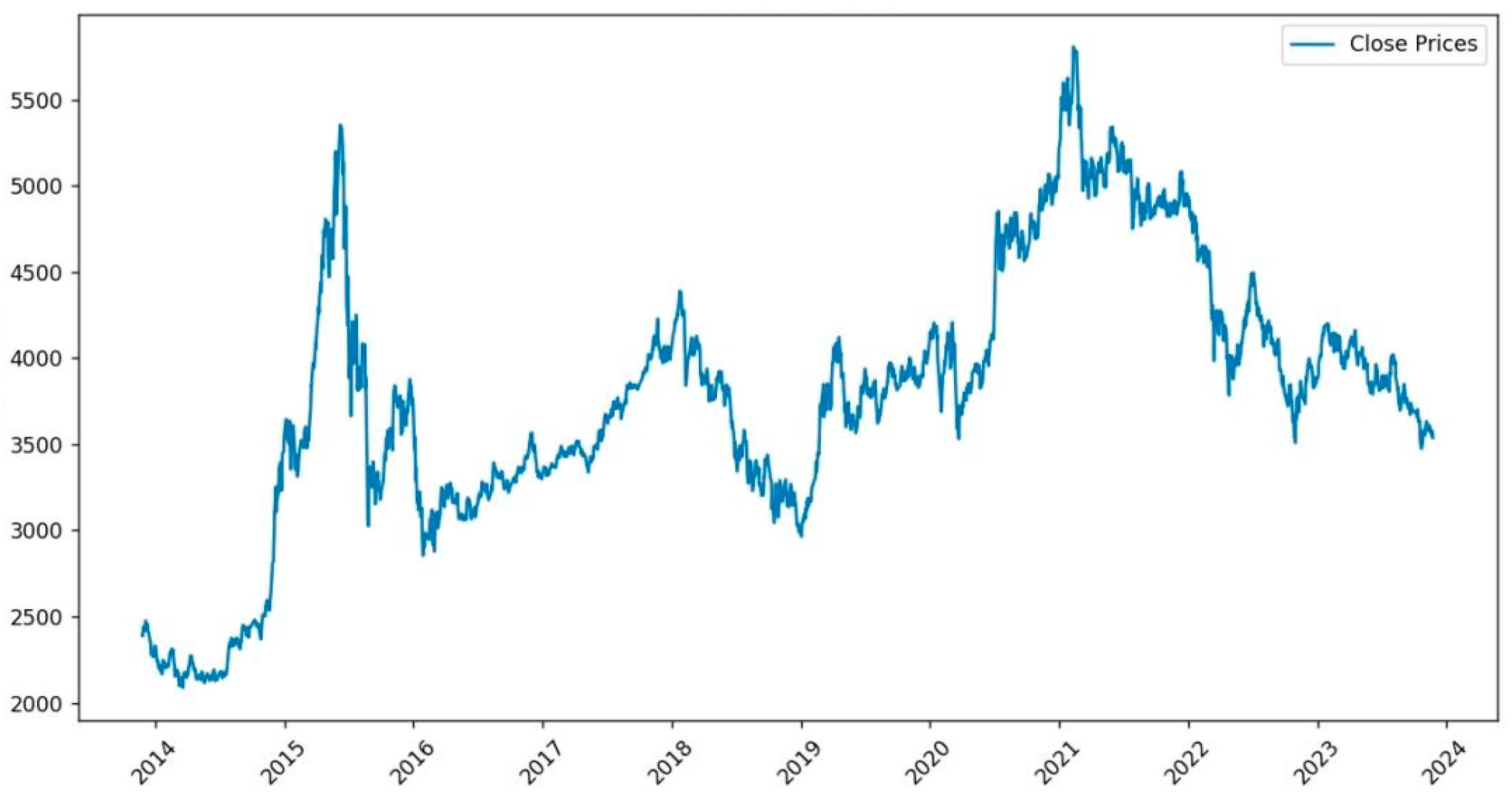
As shown in the time series of closing prices (see Figure 2), the CSI 300 Index surged rapidly in early 2015 but experienced a sharp correction thereafter, entering a prolonged period of volatility. Although there was a brief rebound during 2020–2021, the overall trend remained weak, exhibiting significant uncertainty and structural fluctuations. The combined effects of external shocks and internal market mechanisms have amplified noise in price signals, intensifying the series’ nonlinearity and non-stationarity. Hence, effective denoising and structural feature extraction are essential prerequisites for modeling and forecasting this type of financial time series.

3.2. Correlation Analysis and Dimensionality Reduction

Based on heatmap visualization analysis (see Figure 3), the closing price of the CSI 300 Index shows a strong positive correlation with the opening price, highest price, and lowest price, with correlation coefficients all exceeding 0.99. This indicates a high degree of consistency among these price-related indicators in terms of trend movement. In addition, the closing price exhibits significant co-movement with the On-Balance Volume (OBV) and trading volume, with correlation coefficients of 0.79 and 0.38, respectively. Also, substantial cross-correlations are observed between technical indicators and trading indicators, revealing a high level of information redundancy and multicollinearity in the original feature space. Such characteristics may adversely affect the stability and computational efficiency of downstream models.

To reduce redundant dimensions and improve model performance, this study applies Principal Component Analysis (PCA) to the original set of 13 indicators. Prior to dimensionality reduction, all variables are standardized using z-score normalization to eliminate the influence of inconsistent units and scales across different indicators. The standardization is performed using the following formula:

$$z_i={\displaystyle \frac{x_i-\overline{x}}{s}}$$

(29)

where $x_i$ is the original value, $\overline{x}$ is the sample mean, $s$ is the sample standard deviation, and $z_i$ is the standardized value.

Subsequently, a covariance matrix was computed on the standardized data, followed by eigen decomposition to extract the principal components (see

Table 1. Explained variance of principal components.

Principal Component	Explained Variance	Cumulative Variance
PC1	0.48	0.48
PC2	0.27	0.75
PC3	0.08	0.83
PC4	0.07	0.89
PC5	0.05	0.95
PC6	0.02	0.97
PC7	0.01	0.98
PC8	0.01	0.99
PC9	0.01	0.99

). According to the cumulative explained variance ratio, the first four principal components collectively account for over 85% of the total variance, which indicates that the majority of the structural information in the original data can be retained with minimal loss. As a result, the original 13-dimensional feature space was reduced to 4 principal components, effectively mitigating feature redundancy and achieving clear improvements in both training efficiency and the model’s generalization performance.

4. Results and Analysis

The four extracted principal components were used as input features for the model, while the closing price served as the prediction target. To avoid issues such as gradient instability or impaired convergence due to inconsistent feature scales, the principal components were further normalized to the range $[0,1]$. The normalization formula is as follows:

$$z_i={\displaystyle \frac{x_i-x_{\min }}{x_{\max }-x_{\min }}}$$

(30)

where $x_i$ is the original feature value, $x_{\min }$ and $x_{\max }$ denote the minimum and maximum values of the corresponding feature, respectively. After normalization, the dataset was split into training and testing sets using an 8:2 ratio. The training set was used for model learning and hyperparameter tuning, while the testing set was employed to evaluate the model’s generalization and predictive performance on unseen data.

4.1. Parameters Selection

(1) Wavelet denoising parameters configuration

To improve the stability and effectiveness of data modeling, this study first conducted a statistical examination of the CSI 300 Index closing price. As shown in Figure 4, the distribution of the data exhibits multimodal characteristics and deviates from normality, indicating the presence of notable volatility and noise. Accordingly, denoising is necessary to enhance the quality of the input data.

To better preserve the integrity of stock price waveforms, wavelet bases with higher symmetry should be selected. Among various types, Coiflets wavelets offer notable advantages in signal smoothing and detail extraction. When processing signals with sharp discontinuities, Coiflets can provide a smooth approximation while accurately retaining edge features, effectively minimizing phase distortion during signal reconstruction [35]. This ensures that the denoised data more faithfully reflects actual market trends.

Given that stock price series exhibit both stationary trends and high-frequency fluctuations, this study adopts Coiflets wavelets with vanishing moments of order 4, striking an optimal balance between filter length and reconstruction accuracy. Compared to higher-order configurations, this choice effectively balances noise reduction and feature preservation while avoiding the risk of overfitting high-frequency noise. Additionally, the strong symmetry of Coiflets helps reduce phase shifts during reconstruction, enabling the denoised signal to better preserve local discontinuities and align more closely with real market dynamics.

In practice, a single-level discrete wavelet transform is applied, with a fixed thresholding rule and hard thresholding used for high-frequency coefficients. This configuration outperforms the soft thresholding scheme in terms of RMSE, better retaining the original structural information. After wavelet denoising, local high-frequency disturbances in the original series are effectively suppressed, and the overall trend becomes smoother, meeting the input stability and interpretability requirements of subsequent modeling.

(2) MHABiLSTM model parameters configuration

The MHABiLSTM model enhances the standard BiLSTM architecture by incorporating a multi-head attention mechanism with 8 attention heads, aiming to strengthen the model’s ability to learn long-term dependencies.

The model uses Mean Squared Error (MSE) as the loss function, the Adam optimizer for parameter updates, and the sigmoid function as the activation function. Considering the memory effect of the market while avoiding noise accumulation caused by an excessively long window, the time step was set to 60 trading days in accordance with the characteristics of financial time series. The learning rate was set to 0.001, with a maximum of 100 training epochs and a batch size of 10. To prevent overfitting, early stopping was applied during training. The detailed parameter settings are shown in

Table 2. BiLSTM parameters configuration.

Parameter Name	Value	Symbol
Loss Function	MSE	loss
Optimization Algorithm	Adam	optimizer
Activation Function	sigmoid	activation
Time Step	60	timestep
Learning Rate	0.001	LearnRate
Epochs	100	Epochs
Batch Size	10	batchSize

.

(3) ARIMA model parameters configuration

To correct for the linear trends remaining in the residuals of the MHABiLSTM model, an ARIMA model was introduced for error modeling. The Augmented Dickey–Fuller (ADF) test confirmed that the residual series was stationary ($d=0$), and the Ljung–Box test ruled out the null hypothesis of white noise.

By analyzing the Autocorrelation Function (ACF) and Partial Autocorrelation Function (PACF) plots, the AR and MA orders were determined to be $p=3$ and $q=7$, respectively. Thereby, an ARIMA (3,0,7) model was constructed and applied in a rolling prediction manner to iteratively correct the residual errors of MHABiLSTM, improving the model’s capacity to capture short-term fluctuations.

(4) XGBoost model parameters configuration

The XGBoost model’s hyper-parameters were optimized using grid search, and the best configuration was selected based on 5-fold cross-validation, jointly minimizing the Root Mean Square Error (RMSE) and Mean Absolute Error (MAE).

The final model used gbtree as the base learner and reg:squarederror as the objective function. The optimal parameters are summarized in

Table 3. Optimal hyperparameter settings for the XGBoost model.

Parameter Name	Optimal Value	Search Range	Parameter Symbol
Number of Base Learners	400	[200, 400]	n_estimators
Maximum Tree Depth	3	[3, 4, 5, 6, 7]	max_depth
Minimum Child Weight (leaf node weight threshold)	4	[1, 2, 3, 4, 5]	min_child_weight
Minimum Loss Reduction for Node Splitting (gamma)	0	[0, 0.1]	gamma
Learning Rate	0.1	[0, 0.5]	eta
Objective Function	reg:logistic	reg:squarederror, reg:logistic	objective

.

4.2. Evaluation Metrics

To assess the predictive performance of the models, four commonly used evaluation metrics were employed in this study:

(1) Root Mean Square Error (RMSE)

RMSE measures the magnitude of deviation between predicted and actual values. It emphasizes larger errors by assigning them more weight in the total error. The formula is defined as:

$$\mathrm{RMSE}=\sqrt{{\displaystyle \frac{1}{N}}{\displaystyle \sum _{t=1}^N{({\widehat{y}}_t-y_t)}^2}}$$

(31)

where ${\widehat{y}}_t$ is the predicted value, $y_t$ is the actual value, and $N$ is the total number of samples.

(2) Mean Absolute Percentage Error (MAPE)

MAPE reflects the prediction error as a percentage of the actual value, providing an intuitive interpretation. It is computed as:

$$\mathrm{MAPE}={\displaystyle \frac{100\%}{N}}{\displaystyle \sum _{t=1}^N\left|\frac{{\widehat{y}}_t-y_t}{y_t}\right|}$$

(32)

(3) Mean Absolute Error (MAE)

MAE evaluates the average absolute difference between predicted and actual values. It is defined as:

$$\mathrm{MAE}={\displaystyle \frac{1}{N}}{\displaystyle \sum _{t=1}^N\left|{\widehat{y}}_t-y_t\right|}$$

(33)

(4) Coefficient of Determination (R²)

R² measures the proportion of variance in the dependent variable that is predictable from the independent variables. Its value ranges from 0 to 1, and the closer it is to 1, the better the model fits the data. It is calculated as:

$$R^2=1-{\displaystyle \frac{{\displaystyle \sum _{t=1}^N{\left({\widehat{y}}_t-y_t\right)}^2}}{{\displaystyle \sum _{t=1}^N{\left(y_t-\overline{y}\right)}^2}}}$$

(34)

where $\overline{y}$ is the mean of the actual values.

4.3. Predictive Performance

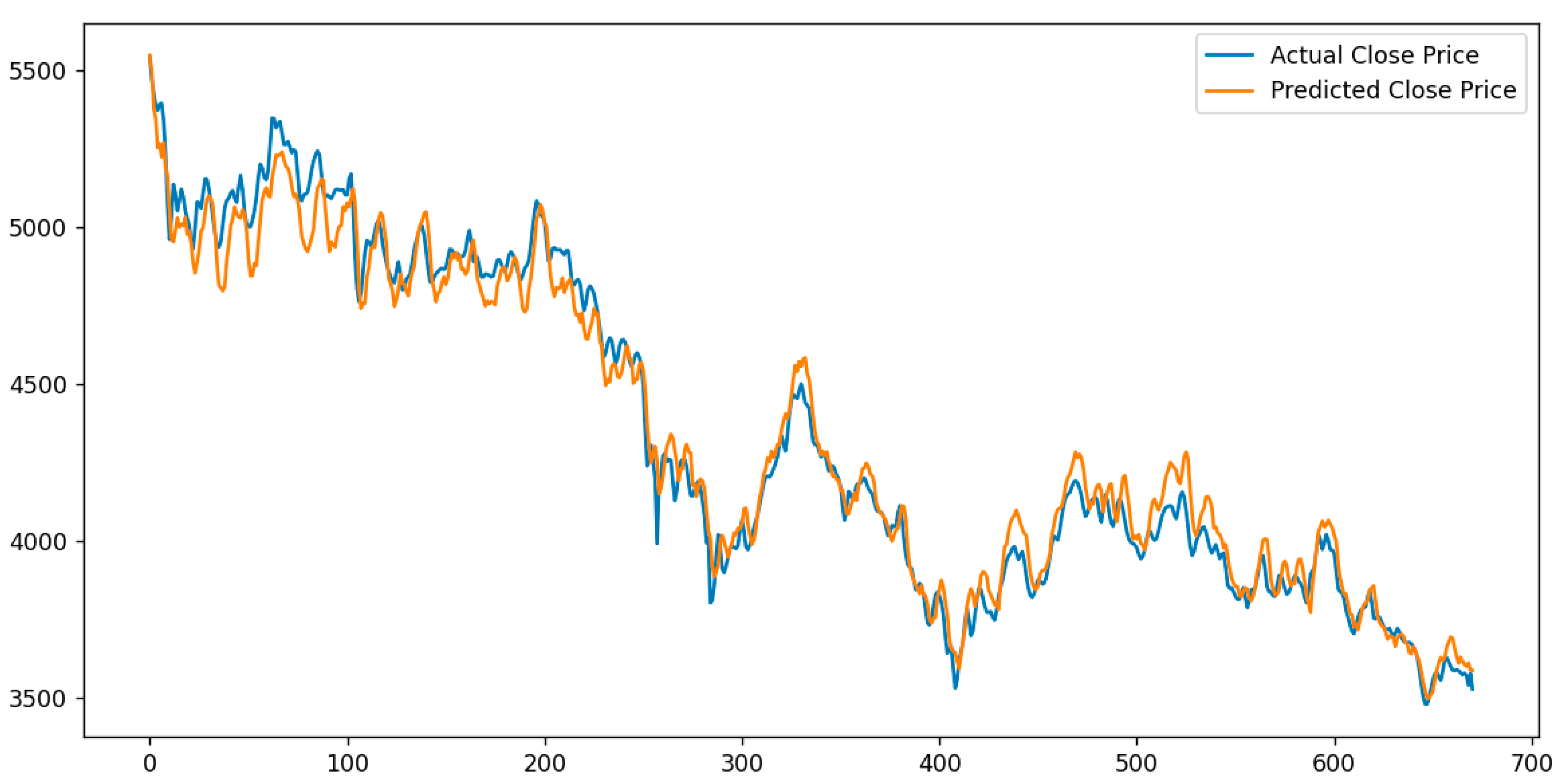
The MHABiLSTM model uses a sliding window approach with a time window of 60 trading days to construct training samples. This design enables the model to effectively capture and fit the long-term trend of stock prices (see Figure 5).

In the testing set, the predicted values of the MHABiLSTM model closely followed the actual stock price trends, demonstrating satisfactory alignment in overall movement (see

Table 4. MHABiLSTM model performance on CSI 300 index.

Method	Metric	Value
MHABiLSTM	RMSE	45.883
	MAE	35.272
	MAPE	0.890
	R2	0.959

). The model achieved an RMSE of 45.883 and an R² of 0.959, indicating robust nonlinear modeling capabilities. However, certain discrepancies were observed in local short-term fluctuations, suggesting that the model may still have limitations in capturing rapid, high-frequency variations.

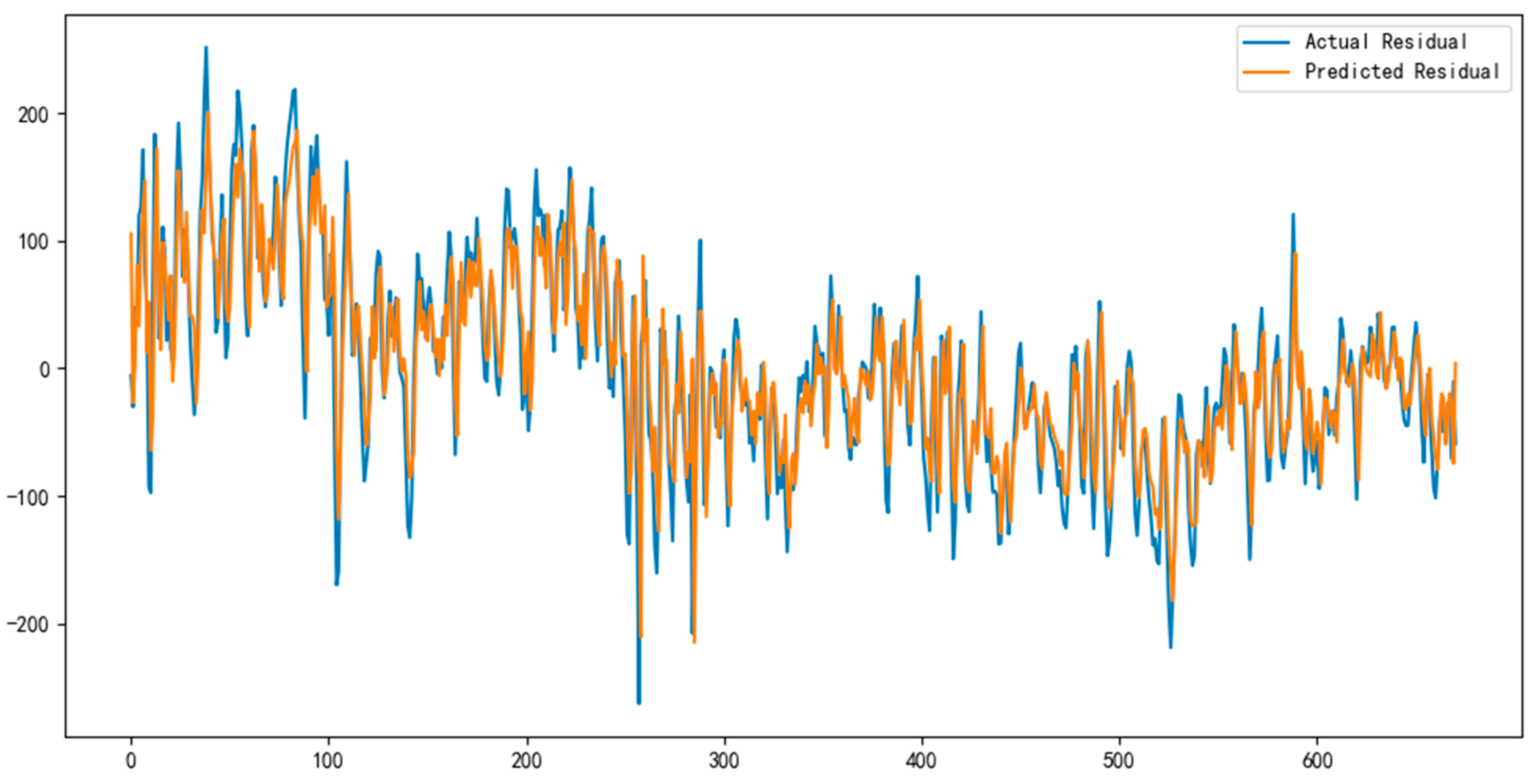
To further address the MHABiLSTM model’s limitations in capturing linear trends, an ARIMA model was applied to its residual sequence (see Figure 6). By extracting the linear trend components from the residuals, the ARIMA model served to correct systematic errors and enhance the overall prediction accuracy.

After training and fitting the ARIMA model, its predicted residuals were added to the MHABiLSTM predictions to obtain the final forecasts of the MHABiLSTM-ARIMA hybrid model. A comparison between the predicted values and the actual values on the test set is illustrated in the Figure 7.

The results in

Table 5. Performance of the MHABiLSTM-ARIMA hybrid model.

Method	Metric	Value
MHABiLSTM-ARIMA	RMSE	41.750
	MAE	31.903
	MAPE	0.805
	R2	0.966

indicate that the MHABiLSTM-ARIMA hybrid model demonstrates clear improvements over the standalone MHABiLSTM model in metrics such as RMSE and MAE. Specifically, the RMSE decreased to 41.750, and the R² increased to 0.966, suggesting that the ARIMA component effectively compensates for the deep learning model’s limitations in capturing linear structures.

By linearly correcting the prediction errors of the MHABiLSTM model using ARIMA, and fusing the results, the RMSE was reduced by 9.01%, and the R² became closer to 1.000. This confirms that ARIMA effectively compensates for MHABiLSTM’s deficiencies in modeling linear trends.

The XGBoost model also demonstrated promising performance in capturing long-term trends. A comparison between the predicted and actual stock prices of the CSI 300 Index on the test set is shown in the Figure 8.

Table 6. Performance of the XGBoost model.

Method	Metric	Value
XGBoost	RMSE	60.793
	MAE	32.107
	MAPE	0.652
	R2	0.988

presents the predictive performance of the XGBoost model on the test dataset. The model achieved an R² of 0.988, demonstrating effective capability in feature extraction. However, due to the lack of explicit temporal structure modeling, the model showed limited ability to capture short-term fluctuations, resulting in a relatively higher RMSE of 60.793.

The XGBoost model demonstrated promising performance in capturing the overall directional movement of CSI 300 stock prices, with outstanding long-term trend fitting. However, it exhibited noticeable bias in modeling short-term fluctuations. As reflected in its accuracy metrics, the MAE reached 32.107, indicating that single-point prediction errors were generally within an acceptable range. Nevertheless, the RMSE climbed to 60.793, suggesting relatively large deviations in certain periods, especially during sharp price swings. XGBoost showed promising performance in error control and long-term trend tracking, but its ability to handle complex short-term volatility was limited. Therefore, integrating sequence-based models to enhance short-term fluctuation modeling, or employing ensemble learning to capture nonlinear trend segments, can further improve forecasting performance.

To this end, the MHABiLSTM-ARIMA and XGBoost model outputs were integrated using the error reciprocal weighting method [36]. This method dynamically allocates greater weight to the model with smaller prediction error on the training set, offering simplicity, adaptability, and effective generalization.

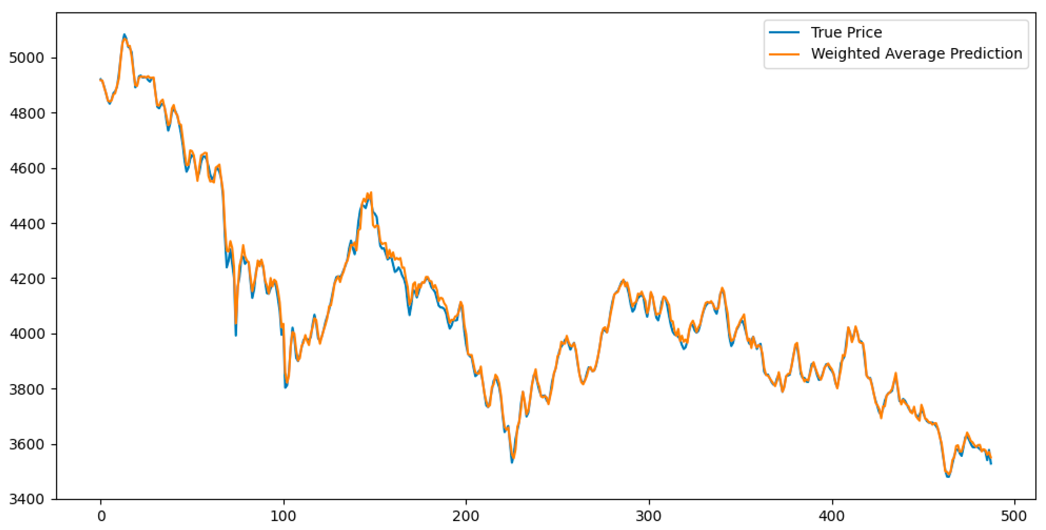
By applying this inverse-error-weighted fusion strategy, the final forecast for CSI 300 stock prices was obtained. Figure 9 illustrates the comparison between the fused predictions and the actual values on the test set, validating the effectiveness of the ensemble strategy in enhancing forecast accuracy and variance explanation.

Table 7. Performance of the MHABiLSTM-ARIMA-XGBoost ensemble model.

Method	Metric	Value
MHABiLSTM-ARIMA-XGBoost	RMSE	20.664
	MAE	21.810
	MAPE	0.488
	R2	0.998

presents the predictive performance of the MHABiLSTM-ARIMA-XGBoost ensemble model on the test dataset. The results show that the model achieves satisfactory accuracy, with an RMSE of 20.664, MAE of 21.810, MAPE of 0.488, and an R² of 0.998, indicating that the ensemble strategy effectively enhances both prediction precision and variance explanation capacity.

The prediction results of the MHABiLSTM-ARIMA-XGBoost ensemble model exhibit a high degree of consistency with the actual trends of the CSI 300 Index, accurately capturing both long-term movements and short-term fluctuations. Among all metrics, the model achieved an RMSE of 20.664, MAE of 21.810, MAPE of 0.488, and an R² value approaching 1, indicating a substantial improvement in prediction accuracy. The improved performance stems from the complete modeling pipeline: wavelet-denoised data were first processed by MHABiLSTM to extract nonlinear patterns, ARIMA was then applied to correct the residual linear trend, and finally, XGBoost was used to integrate predictions through inverse-error weighting. This comprehensive approach outperforms any individual model, validating the accuracy and robustness of the proposed ensemble framework.

The prediction results for the CSI 300 Index further demonstrate notable performance differences among the tested models. A comparative analysis (see

Table 8. Model performance comparison.

Model	RMSE	MAE	MAPE	R2
MHABiLSTM	45.883	32.272	0.890	0.959
MHABiLSTM-ARIMA	41.750	31.903	0.805	0.966
XGBoost	60.793	32.107	0.652	0.988
MHABiLSTM-ARIMA-XGBoost	20.664	21.810	0.488	0.998

) clearly shows that the MHABiLSTM-ARIMA-XGBoost ensemble yields the highest R² and the lowest values for RMSE, MAE, and MAPE, highlighting its superior predictive capabilities. By combining the nonlinear modeling strength of MHABiLSTM, the linear trend-capturing ability of ARIMA, and the feature learning power of XGBoost, the ensemble model effectively leverages the strengths of each component. This hybrid integration clearly enhances its ability to forecast both long-term trends and short-term volatility, delivering better overall performance than any single model.

4.4. Ablation Study

To further validate the effectiveness of each key component in the proposed hybrid model, an ablation study was conducted on the Wavelet-Denoised MHABiLSTM-ARIMA-XGBoost model. By systematically removing one module at a time and observing changes in prediction performance, the contribution of each module to the overall accuracy was evaluated. The full model architecture consists of five core components: Wavelet Denoising, Multi-Head Attention, BiLSTM, ARIMA, and XGBoost. Since XGBoost has already demonstrated effective nonlinear feature extraction capabilities in previous experiments, this ablation focuses on the remaining four components. The results are summarized in

Table 9. Results of the ablation study.

Model Variant	RMSE	MAE	MAPE	R2
Full Model	20.664	21.810	0.488	0.998
w/o Multi-head Attention	22.758	26.787	0.415	0.995
w/o BiLSTM	27.214	22.960	0.491	0.987
w/o ARIMA	33.029	25.951	0.653	0.991
w/o XGBoost	41.750	31.903	0.805	0.966
w/o Wavelet Denoising	27.264	22.520	0.453	0.997

Note: For clarity, each w/o (without) model indicates the removal of the corresponding module from the full model. All ablation models, except for w/o Wavelet Denoising, are based on preprocessing with both Wavelet Denoising and PCA.

.

The results indicate that each module makes a meaningful contribution to the overall predictive performance. Among them, removing the wavelet denoising and ARIMA components caused the most pronounced declines in accuracy, with RMSE increasing by 6.6 and 12.4, respectively. This highlights the critical roles of wavelet-based preprocessing in improving data quality and ARIMA in correcting residual linear trends. In addition, the inclusion of the multi-head attention mechanism and BiLSTM notably enhanced the model’s ability to capture temporal features and improve representational capacity.

4.5. Generalization Capability Validation

To evaluate the proposed ensemble model’s applicability across different financial assets and further verify its stability and generalization capability, an empirical analysis was conducted using individual stock data from Fuyao Glass (600660.SH), in addition to the CSI 300 Index. The dataset spans from 25 November 2013 to 24 November 2023, covering a total of 2436 trading days. Following the same preprocessing pipeline, all models were trained and tested using features derived from wavelet denoising and PCA.

Table 10. Prediction results on Fuyao Glass test set.

Model	RMSE	MAE	MAPE	R2
MHABiLSTM	1.246	0.989	2.623	0.782
MHABiLSTM-ARIMA	0.915	0.672	1.810	0.883
XGBoost	0.902	0.814	1.878	0.954
MHABiLSTM-ARIMA-XGBoost	0.702	0.533	1.414	0.971

presents the predictive results of each model on the Fuyao Glass test set. Compared to the MHABiLSTM model, the MHABiLSTM-ARIMA-XGBoost ensemble reduced RMSE, MAE, and MAPE by 43.6%, 46.1%, and 46.1%, respectively. Relative to XGBoost, the reductions were 22.2%, 34.5%, and 24.7%, respectively. The model also achieved an R² of 0.971, indicating satisfactory fitting performance.

The results demonstrate that the MHABiLSTM-ARIMA-XGBoost model not only performs well on index-level data, but also consistently achieves reliable and stable predictive performance at the individual stock level.

By integrating the strengths of multiple model types, the ensemble effectively captures nonlinear patterns, linear trends, and complex feature interactions in financial time series, validating its robustness and broad applicability across diverse asset classes.

5. Conclusions

This study proposes a hybrid forecasting model for stock price series characterized by high noise, considerable volatility, and non-stationarity. The model integrates wavelet denoising, MHABiLSTM, ARIMA, and XGBoost, effectively combining the nonlinear sequence modeling capacity of BiLSTM, the linear trend correction capability of ARIMA, and the powerful feature representation of XGBoost. The ensemble framework effectively improves prediction accuracy and model stability.

Empirical results on the CSI 300 Index dataset demonstrate that the proposed MHABiLSTM-ARIMA-XGBoost model outperforms both individual models and partial combinations in terms of RMSE, MAE, MAPE, and R². The ablation study further confirms the essential contribution of each component, as the removal of any module leads to performance degradation. Furthermore, experiments on the Fuyao Glass stock dataset demonstrate the model’s promising generalization capability, supporting its applicability to various financial assets.

In summary, the model presented in this study integrates both linear and nonlinear modeling approaches to simultaneously capture the long-term trends and short-term fluctuations of stock price sequences. This dual modeling framework offers a feasible and effective multi-model ensemble path, providing a novel perspective for financial time series forecasting research. Theoretically, this research enriches the literature on multi-model fusion methods and deepens the understanding of the mechanisms underlying the integration of linear and nonlinear dynamics. Practically, the proposed model holds the potential to offer more accurate and stable stock price predictions for investors and financial institutions, thereby supporting investment decision-making and risk management, with promising application prospects.

References

1. Karanasos, M.; Yfanti, S.; Hunter, J. Emerging Stock Market Volatility and Economic Fundamentals: The Importance of US Uncertainty Spillovers, Financial and Health Crises. Ann. Oper. Res. 2022, 313, 1077–1116. [Google Scholar] [CrossRef]
2. Neuhann, D.; Sockin, M. Financial Market Concentration and Misallocation. J. Financ. Econ. 2024, 159, 103875. [Google Scholar] [CrossRef]
3. Song, W.; Zhao, M.; Yu, J. Price Distortion on Market Resource Allocation Efficiency: A DID Analysis Based on National-Level Big Data Comprehensive Pilot Zones. Int. Rev. Econ. Financ. 2025, 102, 104128. [Google Scholar] [CrossRef]
4. Chang, V.; Xu, Q.A.; Chidozie, A.; Wang, H. Predicting Economic Trends and Stock Market Prices with Deep Learning and Advanced Machine Learning Techniques. Electronics 2024, 13, 3396. [Google Scholar] [CrossRef]
5. Rezaei, H.; Faaljou, H.; Mansourfar, G. Stock Price Prediction Using Deep Learning and Frequency Decomposition. Expert. Syst. Appl. 2021, 169, 114332. [Google Scholar] [CrossRef]
6. Sheng, Z.; Liu, Q.; Hu, Y.; Liu, H. A Multi-Feature Stock Index Forecasting Approach Based on LASSO Feature Selection and Non-Stationary Autoformer. Electronics 2025, 14, 2059. [Google Scholar] [CrossRef]
7. Kumbure, M.M.; Lohrmann, C.; Luukka, P.; Porras, J. Machine Learning Techniques and Data for Stock Market Forecasting: A Literature Review. Expert Syst. Appl. 2022, 197, 116659. [Google Scholar] [CrossRef]
8. Mutinda, J.K.; Langat, A.K. Stock Price Prediction Using Combined GARCH-AI Models. Sci. Afr. 2024, 26, e02374. [Google Scholar] [CrossRef]
9. Wang, M. Advanced Stock Market Forecasting: A Comparative Analysis of ARIMA-GARCH, LSTM, and Integrated Wavelet-LSTM Models. SHS Web Conf. 2024, 196, 2008. [Google Scholar] [CrossRef]
10. Oukhouya, H.; El Himdi, K. Comparing Machine Learning Methods—SVR, XGBoost, LSTM, and MLP— for Forecasting the Moroccan Stock Market. Comput. Sci. Math. Forum 2023, 7, 39. [Google Scholar] [CrossRef]
11. Saberironaghi, M.; Ren, J.; Saberironaghi, A. Stock Market Prediction Using Machine Learning and Deep Learning Techniques: A Review. Appliedmath 2025, 5, 76. [Google Scholar] [CrossRef]
12. Sonkavde, G.; Dharrao, D.S.; Bongale, A.M.; Deokate, S.T.; Doreswamy, D.; Bhat, S.K. Forecasting Stock Market Prices Using Machine Learning and Deep Learning Models: A Systematic Review, Performance Analysis and Discussion of Implications. Int. J. Financ. Stud. 2023, 11, 94. [Google Scholar] [CrossRef]
13. Zhang, L.; Hua, L. Major Issues in High-Frequency Financial Data Analysis: A Survey of Solutions. Mathematics 2025, 13, 347. [Google Scholar] [CrossRef]
14. Bao, W.; Cao, Y.; Yang, Y.; Che, H.; Huang, J.; Wen, S. Data-Driven Stock Forecasting Models Based on Neural Networks: A Review. Inf. Fusion 2025, 113, 102616. [Google Scholar] [CrossRef]
15. Liu, Q.; Hu, Y.; Liu, H. Enhanced Stock Price Prediction with Optimized Ensemble Modeling Using Multi-Source Heterogeneous Data: Integrating LSTM Attention Mechanism and Multidimensional Gray Model. J. Ind. Inf. Integr. 2024, 42, 100711. [Google Scholar] [CrossRef]
16. Sha, D.; Zeng, X.; Tran, K.-P.; Xia, L.; Wang, R. A Multi-Granularity Heterogeneous Ensemble Model for Point and Interval Forecasting of Carbon Prices. Int. J. Comput. Intell. Syst. 2025, 18, 142. [Google Scholar] [CrossRef]
17. Sun, Z.; Harit, A.; Cristea, A.I.; Wang, J.; Lio, P. MONEY: Ensemble Learning for Stock Price Movement Prediction via a Convolutional Network with Adversarial Hypergraph Model. AI Open 2023, 4, 165–174. [Google Scholar] [CrossRef]
18. Cui, L.; Chen, Y.; Deng, J.; Han, Z. A Novel attLSTM Framework Combining the Attention Mechanism and Bidirectional LSTM for Demand Forecasting. Expert Syst. Appl. 2024, 254, 124409. [Google Scholar] [CrossRef]
19. Liang, L. ARIMA with Attention-Based CNN-LSTM and XGBoost Hybrid Model for Stock Prediction in the US Stock Market. SHS Web Conf. 2024, 196, 2001. [Google Scholar] [CrossRef]
20. Lv, P.; Wu, Q.; Xu, J.; Shu, Y. Stock Index Prediction Based on Time Series Decomposition and Hybrid Model. Entropy 2022, 24, 146. [Google Scholar] [CrossRef]
21. Li, J.-C.; Sun, L.-P.; Wu, X.; Tao, C. Enhancing Financial Time Series Forecasting with Hybrid Deep Learning: CEEMDAN-Informer-LSTM Model. Appl. Soft Comput. 2025, 177, 113241. [Google Scholar] [CrossRef]
22. Zhao, C.; Cai, J.; Yang, S. A Hybrid Stock Prediction Method Based on Periodic/Non-Periodic Features Analyses. EPJ Data Sci. 2025, 14, 1. [Google Scholar] [CrossRef]
23. Lin, B.; Bai, R. Machine Learning Approaches for Explaining Determinants of the Debt Financing in Heavy-Polluting Enterprises. Finance Res. Lett. 2022, 44, 102094. [Google Scholar] [CrossRef]
24. Wang, X.; Zhang, B.; Xu, Z.; Li, M.; Skare, M. A Multi-Dimensional Decision Framework Based on the XGBoost Algorithm and the Constrained Parametric Approach. Sci. Rep. 2025, 15, 4315. [Google Scholar] [CrossRef] [PubMed]
25. Rubio, L.; Palacio Pinedo, A.; Mejía Castaño, A.; Ramos, F. Forecasting Volatility by Using Wavelet Transform, ARIMA and GARCH Models. Eurasian Econ. Rev. 2023, 13, 803–830. [Google Scholar] [CrossRef]
26. Zhang, J.; Liu, H.; Bai, W.; Li, X. A Hybrid Approach of Wavelet Transform, ARIMA and LSTM Model for the Share Price Index Futures Forecasting. North Am. J. Econ. Financ. 2024, 69, 102022. [Google Scholar] [CrossRef]
27. Kılıç, D.K.; Uğur, Ö. Hybrid Wavelet-Neural Network Models for Time Series. Appl. Soft Comput. 2023, 144, 110469. [Google Scholar] [CrossRef]
28. Ouyang, C.; Cai, L.; Liu, B.; Zhang, T. An Improved Wavelet Threshold Denoising Approach for Surface Electromyography Signal. EURASIP J. Adv. Signal Process. 2023, 2023, 108. [Google Scholar] [CrossRef]
29. Kontopoulou, V.I.; Panagopoulos, A.D.; Kakkos, I.; Matsopoulos, G.K. A Review of ARIMA vs. Machine Learning Approaches for Time Series Forecasting in Data Driven Networks. Future Internet 2023, 15, 255. [Google Scholar] [CrossRef]
30. Hochreiter, S.; Schmidhuber, J. Long Short-Term Memory. Neural Comput. 1997, 9, 1735–1780. [Google Scholar] [CrossRef]
31. Feng, Z.; Zhang, J.; Niu, W. A State-of-the-Art Review of Long Short-Term Memory Models with Applications in Hydrology and Water Resources. Appl. Soft Comput. 2024, 167, 112352. [Google Scholar] [CrossRef]
32. Niu, Z.; Zhong, G.; Yu, H. A Review on the Attention Mechanism of Deep Learning. Neurocomputing 2021, 452, 48–62. [Google Scholar] [CrossRef]
33. Vaswani, A.; Shazeer, N.; Parmar, N.; Uszkoreit, J.; Jones, L.; Gomez, A.N.; Kaiser, L.; Polosukhin, I. Attention Is All You Need. arXiv 2023, arXiv:1706.03762. [Google Scholar]
34. Chen, T.; Guestrin, C. XGBoost: A Scalable Tree Boosting System. In Proceedings of the 22nd ACM SIGKDD International Conference on Knowledge Discovery and Data Mining, San Francisco, CA, USA, 13 August 2016; pp. 785–794. [Google Scholar]
35. Elias, I.I.; Ali, T.H. Optimal Level and Order of the Coiflets Wavelet in the VAR Time Series Denoise Analysis. Front. Appl. Math. Stat. 2025, 11, 1526540. [Google Scholar] [CrossRef]
36. Sun, X.; Yin, J.; Zhao, Y. Using the Inverse of Expected Error Variance to Determine Weights of Individual Ensemble Members: Application to Temperature Prediction. J. Meteorol. Res. 2017, 31, 502–513. [Google Scholar] [CrossRef]
Figure 1. LSTM structure.
Mathematics 13 02622 g001
Figure 2. The closing price of the CSI 300 stock index.
Mathematics 13 02622 g002
Figure 3. Indicator heatmap.
Mathematics 13 02622 g003
Figure 4. Histogram of closing prices (left) and normal probability diagram (right).
Mathematics 13 02622 g004
Figure 5. MHABiLSTM predictions for CSI 300 stock index.
Mathematics 13 02622 g005
Figure 6. Predicted results of the ARIMA model.
Mathematics 13 02622 g006
Figure 7. Forecasting performance of the MHABiLSTM-ARIMA hybrid model.
Mathematics 13 02622 g007
Figure 8. Predicted results of the XGBoost model.
Mathematics 13 02622 g008
Figure 9. Predicted results of the MHABiLSTM-ARIMA-XGBoost ensemble model.
Mathematics 13 02622 g009