Traffic Characterization Based on Driver Reaction

Abstract

A macroscopic model for nonhomogeneous traffic is introduced that incorporates relaxation time and lateral time headway, and accounts for driver reaction time. Driver reaction is based on models of real-world nonhomogeneous traffic flow in Pakistan and Iran. A lateral time headway model is obtained using lane change data to characterize traffic during lane changes. The performance of the proposed model is compared with the well-known Payne–Whitham (PW) model on a 3000 m circular road using the FORCE numerical scheme. The results show that the initial multi-cluster density distribution evolves more realistically and accurately with the proposed model. Thus, it can be used to aid in traffic congestion mitigation for on-ramps and off-ramps.

1. Introduction

Precise characterization of traffic dynamics is crucial to effectively model congestion. This study introduces a traffic model that captures the evolution of traffic with a multi-cluster density distribution. This type of distribution results in large fluctuations in traffic behavior, which causes congestion and reduces efficiency [1]. The relaxation time is the time for drivers to adapt to a desired velocity based on the velocity and density [2]. It influences the responsiveness, stability, and accuracy of traffic models, leading to better traffic flow analysis, policy-making, and infrastructure design. The lateral time headway is the time between two adjacent vehicles traveling in parallel lanes. It affects lane changes, merging at ramps, weaving sections, highway safety, and autonomous vehicle decisions. During congestion, the lateral time headway is small, as vehicles are tightly packed. Consequently, lane changes are difficult and less frequent, as drivers have fewer acceptable gaps. This is important in merging zones, intersections, and bottlenecks where lateral interactions dominate. Both relaxation time and time headway are essential to model real-world congestion behavior.

Traffic flow can be classified as homogeneous or nonhomogeneous. In homogeneous traffic, vehicle types are similar and drivers typically adhere to lane discipline, resulting in minimal fluctuations in speed and density. On the other hand, nonhomogeneous traffic often lacks lane discipline and includes a mix of motorized and non-motorized vehicles [3]. This disrupts the smooth flow of traffic and frequently leads to bottlenecks and congestion [4]. Nonhomogeneous traffic is more complex and thus more difficult to characterize [5]. However, understanding this traffic is crucial for developing efficient traffic management strategies [6]. Conventional methods are primarily designed for homogeneous traffic and therefore perform poorly with nonhomogeneous traffic [7].

Traffic conditions on a road influence driver response [8]. For example, maintaining a safe distance headway from the vehicle ahead is crucial to avoid collisions [9]. In congestion, vehicles are closer together and there is frequent acceleration and deceleration [10]. A small lateral time headway increases the risk of collisions, especially during congestion, ramp merging, and lane changes. Drivers maintain a safe lateral time headway to prevent accidents [11], and this reduces driver conflicts and vehicle interactions. Typically, the safe lateral time headway is between 1.5 s and 3 s [12]. In nonhomogeneous traffic, the relaxation time and headway can vary significantly due to the lack of lane discipline. As a result, accurately representing this traffic requires a model that considers both relaxation time and lateral time headway.

Traditional macroscopic traffic models such as the Payne–Whitham (PW) model assume that traffic adapts instantaneously, and relaxation is ignored [13,14]. Further, traffic is considered to be homogeneous and behavior is uniform, and the lateral distance headway and lateral time headway are ignored [15,16]. Thus, they are not suitable for nonhomogeneous traffic, which is typical in developing countries. Therefore, a traffic model is proposed that considers both the relaxation time and time headway to accurately characterize traffic behavior. In particular, the PW model is modified to include driver reaction based on these parameters. The traffic flow is modeled using data obtained in Pakistan, while the time headway is modeled using data from Iran. The proposed and PW models are evaluated over a 3000 m circular road for 300 s. A multi-cluster density distribution is used to represent nonhomogeneous traffic. The results show that the proposed model provides a more realistic characterization of nonhomogeneous traffic.

The rest of this paper is organized as follows. A review of the related literature is presented in Section 2. The proposed macroscopic traffic model is given in Section 3. The hyperbolicity of the proposed and PW models is examined in Section 4. Section 5 introduces the FORCE scheme, and Section 6 provides the corresponding convergence analysis. The performance of the proposed and PW models is evaluated in Section 7. Finally, some conclusions are presented in Section 8.

2. Literature Review

Macroscopic traffic models are based on aggregate traffic parameters such as velocity, density, and flow [17]. They are used to examine the overall behavior of traffic and are suitable for large-scale traffic systems such as urban networks and highways. These models are widely used for congestion analysis, infrastructure planning, and traffic control. Microscopic models focus on individual vehicle behavior [18,19]. They focus on car-following, lane-changing, and acceleration/deceleration decisions, and they consider factors such as driver behavior, perception, and reaction time. Microscopic models are useful for intersections, ramps, and mixed traffic [20]. Mesoscopic traffic models combine elements of both macroscopic and microscopic models [21]. They are typically used to model traffic flows using probabilistic parameters [17,22]. Microscopic models have high computational complexity but can provide detailed results. Conversely, macroscopic models are simple and have low complexity, and so are widely employed [18,23].

The Lighthill, Whitham, and Richards (LWR) model [13,14] is a first-order model given as follows:

$${\displaystyle \frac{\partial \rho }{\partial t}}+{\displaystyle \frac{\partial \left(\rho v\right(\rho \left)\right)}{\partial x}}=0,$$

(1)

where x is distance, t is time, ρ is the density, and v(ρ) is the desired velocity based on the density for uniform traffic. This model characterizes traffic dynamics using the law of conservation and considers traffic as a fluid. It is very simple and can be employed for congestion and freeway control, and real-time traffic management. However, the LWR model assumes homogeneous traffic and cannot accurately model stop-and-go traffic [24]. Further, driver reaction is ignored and vehicle alignment is instantaneous, so relaxation time and time headway are not considered. This model is not suitable for large changes in traffic [15,16], interactions at intersections, and lane changes.

Payne proposed a higher-order model by adding velocity and driver response (reaction) [4,25]. The first equation is based on vehicle conservation as in the LWR model. Driver response to changes in traffic is based on a constant unrelated to traffic physics, so driver behavior and traffic conditions are ignored [8]. A relaxation term is used for changes while achieving the desired velocity [16]. Whitham independently developed this model, and so it is referred to as the Payne–Whitham (PW) model [8]:

$$\begin{array}{ccc}\hfill {\displaystyle \frac{\partial \rho }{\partial t}}+{\displaystyle \frac{\partial }{\partial x}}\left(\rho v\left(\rho \right)\right)& =& 0,\hfill \\ \hfill {\displaystyle \frac{\partial \left(\rho v\right)}{\partial t}}+{\displaystyle \frac{\partial }{\partial x}}\left({\displaystyle \frac{{\left(\rho v\right)}^2}{\rho }}+C_0^2\rho \right)& =& \rho \left({\displaystyle \frac{v\left(\rho \right)-v}{\tau }}\right),\hfill \end{array}$$

(2)

where ${\displaystyle \frac{\partial \left(\rho v\right)}{\partial t}}$ represents the temporal change in traffic flow. When ${\displaystyle \frac{\partial \left(\rho v\right)}{\partial t}}<0$, the flow is decreasing, while for ${\displaystyle \frac{\partial \left(\rho v\right)}{\partial t}}>0$, it is increasing. The term ${\displaystyle \frac{{\left(\rho v\right)}^2}{\rho }}$ characterizes the changes in downstream traffic, and $C_0^2\rho$ is the driver reaction, which is based on a constant, C₀. The term ${\displaystyle \frac{\partial }{\partial x}}\left({\displaystyle \frac{{\left(\rho v\right)}^2}{\rho }}+C_0^2\rho \right)$ in the PW model provides traffic stability. ${\displaystyle \frac{v\left(\rho \right)-v}{\tau }}$ is the relaxation term and τ is the relaxation time. The alignment to forward traffic is quicker with a small τ value, while changes in traffic are greater with a large τ value. As C₀ is a constant, the density and velocity behavior are the same regardless of the traffic conditions, which is not realistic [26]. Consequently, this model provides unsatisfactory results during congestion [4]. A model should account for human factors such as relaxation time and lateral time headway.

The PW model can produce oscillatory behavior when there are large changes in traffic. Thus, a term was added to mitigate these effects, but the results are unsatisfactory for abrupt changes in traffic [27]. The PW model was also improved in [28]. However, small changes in speed and density can grow over time, which causes vehicles to group together, resulting in stop-and-go traffic without bottlenecks or accidents. Thus, vehicles evolve into groups during homogeneous flow without external factors.

Although the LWR and PW models have been used in a variety of applications, homogeneous traffic is assumed, so they do not reflect the diversity of real-world driving, and they cannot capture on-ramp and off-ramp behavior. Furthermore, calibration of these models is challenging, as precise traffic data is required, which can be difficult to obtain [29]. A macroscopic model based on velocity variance was proposed in [30], which is derived from Gas-Kinetic Theory (GKT). However, the model parameters are difficult to interpret. The PW model was modified in [31] by including driver reaction time, but when the density is high, instability can occur, resulting in stop-and-go traffic. The greater the reaction time, the more likely traffic becomes unstable, regardless of external factors.

A model based on GKT was developed in [32], where the relaxation time τ is a function of traffic density. However, statistical distributions are used, which increases the model complexity, and the analogy with gas theory is uncertain. Traffic is influenced by conditions ahead of a vehicle, and changes in velocity tend to be less than the average speed [15]. The PW model cannot account for the impact of leading vehicles [33], so speeds can be unrealistic when the density is high [34,35], but it can be suitable for multi-lane traffic [36].

In [37], a modified PW model based on vehicle density was given. However, density is assumed to be a monotonic increasing function regardless of driver response [38,39], which is not realistic. Further, homogeneous traffic is assumed, and the impact of different vehicle types is ignored. The PW model was improved in [4] by considering density-dependent velocity changes, but driver reaction is based on the desired velocity and adapts instantaneously to conditions ahead. This model also ignores parallel traffic and the time for a driver to react to changes ahead. Thus, lateral interactions between parallel and forward vehicles are ignored. The PW model was improved in [23] to consider nonhomogeneous traffic based on time headway and lateral distance. These parameters are important when there is a lack of lane discipline.

The desired velocity is a function of density and velocity and decreases as density increases [6,40]. The Greenshields velocity model [23] is widely used and is given as follows:

$$v\left(\rho \right)=v_m\left(1-{\displaystyle \frac{\rho }{{\rho }_m}}\right),$$

(3)

where v_m and ρ_m are the maximum velocity and density, respectively. This model can be used for nonhomogeneous traffic because the relationship is nonlinear [41]. A logarithmic relationship between density and speed was considered in [42], and an exponential relationship was proposed in [43] based on traffic data from the Merritt Parkway in Connecticut, USA. However, the velocity can be unrealistic.

The above results indicate that a macroscopic traffic model based on relaxation time and time and distance headway is required to accurately predict traffic behavior. Driver reaction to forward changes should incorporate these parameters, as they are based on traffic physics.

3. Traffic Models

Density is a key factor in traffic behavior [44]. Driver reaction is fast with a large density and slow for a small relaxation time τ. However, changes in flow increase with the relaxation time. Thus, driver reaction can be expressed as follows:

$$D_R={\displaystyle \frac{1}{\tau }}{\displaystyle \frac{\partial f}{\partial \rho }},$$

(4)

where f = ρv is the flow. Substituting $\Delta v={\displaystyle \frac{\partial f}{\partial \rho }}$ in (4) gives

$$D_R={\displaystyle \frac{1}{\tau }}\Delta v,$$

(5)

so driver reaction is affected by changes in velocity during the relaxation time τ. The reaction is quick with a large change in velocity and short relaxation time and slow with a small change in velocity and a large relaxation time. In free-flow traffic, vehicle interactions are slow, as there is sufficient time to react to changes in velocity [8].

Traffic data was collected for the week of Monday, 10 January 2022 to Sunday, 16 January 2022, from a sensor node in Peshawar, Pakistan, located at 33.99841270487691 latitude and 71.47962908395094 longitude [20]. This is a nonhomogeneous traffic environment where vehicles lack lane discipline. The time span was 9 a.m. to 4 p.m. each day to cover the congestion period. The node is based on a Raspberry Pi (RPi) 4 and has a Pi Camera v2 connected via the CSI port to record 1080p video at 20 frames per second. An Intel Movidius Neural Compute Stick 2 was integrated with the RPI 4 for edge computation. The count accuracy was 93.2% and the speed prediction accuracy was 82.9% [45]. 10,000 vehicles per day were considered in the analysis. The interquartile range was used to remove outliers from the data. Linear, exponential, logarithmic, power, and quadratic polynomial models were fit to the vehicle flow $f\left(\rho \right)$ and density ρ data. The best fit model for the flow is [20]

$$f\left(\rho \right)=-44.34{\rho }^2+80.02\rho +1.63,$$

(6)

with R² = 0.7159. The negative coefficient of ρ² indicates that the relationship between flow and density is concave downward, i.e., flow increases with density up to a point and then decreases as congestion occurs. The constant 1.628 is the minimum flow, which corresponds to the minimum density.

The change in flow with respect to density from (6) is as follows:

$$\Delta v={\displaystyle \frac{\partial f\left(\rho \right)}{\partial \rho }}=-88.68\rho +80.02.$$

(7)

Density is the number of vehicles per unit length and is measured in vehicles per meter. Then, the lateral distance between vehicles covered during a lane change can be expressed as follows:

$$\rho ={\displaystyle \frac{1}{h_d}}.$$

(8)

Then, from (8) and (7), we have

$${\displaystyle \frac{\partial f}{\partial \rho }}={\displaystyle \frac{-88.68}{h_d}}+80.02,$$

(9)

and

$$h_d=v_{n}h,$$

(10)

where h is the required lateral time headway for normalized velocity v_n to change lanes.

The lateral time headway is modeled using data for lane changes on the Tehran–Karaj freeway in Iran [12]. On this road, 35% of the vehicles overtake each other, and the traffic is nonhomogeneous. The length of the road observed is 100 m, and HD (1280 × 720) video was provided by the Bureau of Rural Road and Transportation. Vehicle motion was determined using Python 2.2 and the OpenCV library, and vehicle tracking was performed using the Kernelized Correlation Filter (KCF) algorithm. Over a 5 h period, 2580 vehicles were selected and 92,278 data values were obtained. The speeds ranged from 61 to 127 km/h with an average of 97 km/h. The average time headway was 0.9 s with a maximum of 3.24 s. Driving behavior was categorized based on lateral distance. For lateral distances <0.50 m, traffic is lane based, while for lateral distances between 0.50 m and 2.20 m, it is non-lane based. The model obtained is

$$h=0.003d+1.22,$$

(11)

where the coefficient 0.003 indicates that the lateral time headway increases with the lateral distance headway d, and 1.22 is the minimum lateral time headway between parallel vehicles.

The traffic flow and lateral time headway models obtained can be used to accurately predict traffic behavior. They show that high-speed traffic with a low density does not result in a large driver reaction to slow-moving traffic. Thus, changes in the traffic do not grow, but rather decay spatially and temporally. During lane changes, movement is controlled, so speed variations are small, as expected. In addition, including both models provides a better characterization of stop-and-go traffic. Substituting h from (11) in (10) gives

$$h_d=v_n(0.003d+1.22),$$

(12)

and then substituting (12) in (9) results in

$$\Delta v={\displaystyle \frac{-88.68}{v_n(0.003d+1.22)}}+80.02.$$

(13)

This indicates that changes in velocity depend on the lateral distance headway and road location. With a large lateral distance headway, changes in velocity are large, as collisions are less likely.

Lane discipline is typically lacking in nonhomogeneous traffic [46], so the lateral distance headway is small. However, in homogeneous traffic, there is often lane discipline, so the lateral distance headway is larger. Substituting (13) in (5) gives the driver reaction:

$$D_R={\displaystyle \frac{1}{\tau }}\left({\displaystyle \frac{-88.68}{v_n(0.003d+1.22)}}+80.02\right).$$

(14)

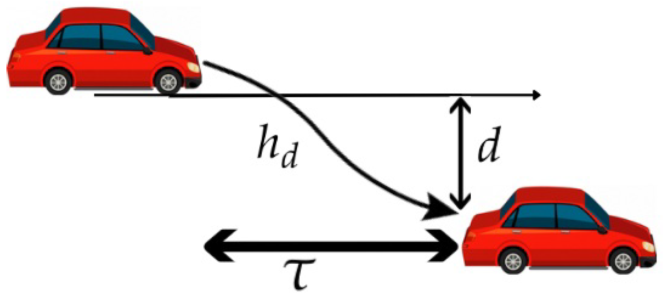
This shows that driver reaction is greater for a larger distance headway, and smaller changes in traffic are expected. Further, with a small relaxation time, driver reaction is fast, and typically, traffic is free-flow. With a larger relaxation time, driver reaction is slow, which is typical in congestion. Figure 1 illustrates the relaxation time, distance covered during a lane change, and lateral distance headway. Substituting D_R from (14) for C₀ in (2) gives the following:

$$\begin{array}{ccc}\hfill {\displaystyle \frac{\partial \rho }{\partial t}}+{\displaystyle \frac{\partial }{\partial x}}\left(\rho v\left(\rho \right)\right)& =& 0,\hfill \\ \hfill {\displaystyle \frac{\partial \left(\rho v\right)}{\partial t}}+{\displaystyle \frac{\partial }{\partial x}}\left({\displaystyle \frac{{\left(\rho v\right)}^2}{\rho }}+\left[{\left({\displaystyle \frac{1}{\tau }}\left({\displaystyle \frac{-88.68}{v_n(0.003d+1.22)}}+80.02\right)\right)}^2\rho \right]\right)& =& \rho \left({\displaystyle \frac{v\left(\rho \right)-v}{\tau }}\right).\hfill \end{array}$$

(15)

This characterizes both homogeneous and nonhomogeneous traffic considering driver reaction. Large changes in traffic are expected with a small driver reaction, while the changes are small with a large driver reaction. The first equation in (15) is the same as in the PW model (2).

Table 1. Driver response for the PW and proposed traffic models.

PW Model	Proposed Model
$C_0^2\rho$	${\left({\displaystyle \frac{1}{\tau }}\left({\displaystyle \frac{-88.68}{v_n(0.003d+1.22)}}+80.02\right)\right)}^2\rho$

gives the driver response for the PW and proposed models from (2) and (15), respectively. This shows that driver response with the proposed model depends on the relaxation time and lateral distance between vehicles. Conversely, driver response with the PW model is based on the constant C₀.

4. Traffic Model Hyperbolicity

A traffic system is required to be hyperbolic [15,16]. This ensures a unique solution exists for realistic initial and boundary conditions, and small measurement errors do not result in significant differences in traffic characterization, so the solution is well posed [8,39]. Further, hyperbolic systems have stable numerical solutions with the first-order centered (FORCE) scheme [47], i.e., they converge and produce realistic results [48]. The eigenvalues of a hyperbolic traffic system are unique and real [49]. The conserved model in divergence form is used to find the eigenvalues and is given as follows:

$${\displaystyle \frac{\partial \zeta }{\partial t}}+{\displaystyle \frac{\partial f\left(\zeta \right)}{\partial x}}=S\left(\zeta \right).$$

(16)

The variables ρ and ρv are conserved, which ensures numerical stability so the traffic flow is consistent.

The PW model based on the conserved variables is as follows: [23]

$$\zeta =\left(\begin{array}{c}\rho \\ \rho v\end{array}\right),f\left(\zeta \right)=\left(\begin{array}{c}\rho v\\ {\displaystyle \frac{{\left(\rho v\right)}^2}{\rho }+C_0^2\rho }\end{array}\right),S\left(\zeta \right)=\left(\begin{array}{c}0\\ {\displaystyle \rho \frac{v\left(\rho \right)-v}{\tau }}\end{array}\right),$$

(17)

while the proposed model based on these variables is

$$\zeta =\left(\begin{array}{c}\rho \\ \rho v\end{array}\right),f\left(\zeta \right)=\left(\begin{array}{c}\rho v\\ {\displaystyle \frac{{\left(\rho v\right)}^2}{\rho }+{\left(\frac{1}{\tau }\left(\frac{-88.68}{v_n(0.003d+1.22)}+80.02\right)\right)}^2\rho }\end{array}\right),S\left(\zeta \right)=\left(\begin{array}{c}0\\ {\displaystyle \rho \frac{v\left(\rho \right)-v}{\tau }}\end{array}\right).$$

(18)

This quasilinear system depends on driver reaction for traffic alignment to forward vehicles and ignores relaxation, so $S\left(\zeta \right)=0$ and (16) takes the following form:

$${\displaystyle \frac{\partial \zeta }{\partial t}}+{\displaystyle \frac{\partial f\left(\zeta \right)}{\partial x}}=0.$$

(19)

The Jacobian matrix quantifies model sensitivity to small changes and determines the propagation of traffic changes. It provides the gradients of the vector $f\left(\zeta \right)$ with the conserved traffic variables. The Jacobian matrix for the PW model is

$$A={\displaystyle \frac{\partial }{\partial (\rho ,\rho v)}}\left(\begin{array}{c}\rho v\\ {\displaystyle \frac{{\left(\rho v\right)}^2}{\rho }}+C_0^2\rho \end{array}\right),$$

(20)

which takes the form

$$A\left(\zeta \right)=\left(\begin{array}{cc}0& 1\\ -v^2+C_0^2& 2v\end{array}\right).$$

(21)

The eigenvalues are the solutions of [23]

$$\left|A\left(\zeta \right)-\lambda I\right|=\left|\begin{array}{cc}-\lambda & 1\\ -v^2+C_0^2& 2v-\lambda \end{array}\right|,$$

(22)

which are

$${\lambda }_1=v+C_0,{\lambda }_2=v-C_0.$$

(23)

These eigenvalues are distinct and real, so the PW model is hyperbolic and is a well-posed traffic system. The changes in flow propagate according to λ_1,2, and do not increase unbounded over time. λ₁ characterizes free-flow traffic, while λ₂ characterizes congested traffic. Thus, changes in flow occur according to the constant C₀, which is not based on traffic physics.

The Jacobian matrix for the proposed model is

$$A={\displaystyle \frac{\partial }{\partial (\rho ,\rho v)}}\left(\begin{array}{c}\rho v\\ \frac{{\left(\rho v\right)}^2}{\rho }+{\left({\displaystyle \frac{1}{\tau }}\left({\displaystyle \frac{-88.68}{v_n(0.003d+1.22)}}+80.02\right)\right)}^2\rho \end{array}\right),$$

(24)

which takes the form

$$A\left(\zeta \right)=\left(\begin{array}{cc}0& 1\\ -v^2+{\left({\displaystyle \frac{1}{\tau }}\left({\displaystyle \frac{-88.68}{v_n(0.003d+1.22)}}+80.02\right)\right)}^2& 2v\end{array}\right).$$

(25)

The eigenvalues are the solutions of

$$\left|A\left(\zeta \right)-\lambda I\right|=\left|\begin{array}{cc}-\lambda & 1\\ -v^2+{\left({\displaystyle \frac{1}{\tau }}\left({\displaystyle \frac{-88.68}{v_n(0.003d+1.22)}}+80.02\right)\right)}^2& 2v-\lambda \end{array}\right|,$$

(26)

which are

$${\lambda }_1=v+{\displaystyle \frac{1}{\tau }}\left({\displaystyle \frac{-88.68}{v_n(0.003d+1.22)}}+80.02\right),{\lambda }_2=v-{\displaystyle \frac{1}{\tau }}\left({\displaystyle \frac{-88.68}{v_n(0.003d+1.22)}}+80.02\right).$$

(27)

These eigenvalues are distinct and real, so the proposed model is hyperbolic. They indicate that changes in flow are a function of the time headway and relaxation time. Thus, traffic behavior will be more realistic than with the PW model and based on traffic physics.

5. FORCE Numerical Scheme

The proposed and PW models are implemented in MATLAB R2019b using the First Order Centered (FORCE) scheme [47]. This technique has previously been used for traffic systems [50], as it can approximate large traffic changes and produce accurate results. Further, the computational complexity is lower than the Roe scheme [50], and it is simple to implement. The FORCE scheme is based on the second-order Richtmyer and first-order Lax–Friedrichs methods.

The road of length x_M is divided into M equally spaced segments, so each segment has length

$$\delta x={\displaystyle \frac{x_M}{M}}.$$

The simulation time t_N is divided into N discrete time steps, so each time step is

$$\delta t={\displaystyle \frac{t_N}{N}}=t_{n+1}-t_n.$$

At each time step, the variables ζ and $f\left(\zeta \right)$ for the proposed and PW models given by (18) and (17), respectively, are approximated over each road segment given by the interval $\left(x_i-{\displaystyle \frac{\delta x}{2}},x_i+{\displaystyle \frac{\delta x}{2}}\right)$.

Let ζ denote the average value of the data variables within the ith road segment. Using the Lax–Friedrichs scheme, the traffic flux at the boundary between segments i and i + 1 is given by

$${\left(f_{i+{\displaystyle \frac{1}{2}}}^n({\zeta }_i^n,{\zeta }_{i+1}^n)\right)}^l={\displaystyle \frac{1}{2}}\left(f\left({\zeta }_i^n\right)+f\left({\zeta }_{i+1}^n\right)\right)+{\displaystyle \frac{1}{2}}{\displaystyle \frac{\delta t}{\delta x}}({\zeta }_i^n-{\zeta }_{i+1}^n),$$

(28)

where the superscript l indicates the Lax–Friedrichs scheme. For the Richtmyer scheme, the intermediate value of the data variables at the segment interface is

$${\left({\zeta }_{i+{\displaystyle \frac{1}{2}}}\right)}^r={\displaystyle \frac{1}{2}}\left({\zeta }_i^n+{\zeta }_{i+1}^n\right)+{\displaystyle \frac{1}{2}}{\displaystyle \frac{\delta t}{\delta x}}\left(f\left({\zeta }_i^n\right)-f\left({\zeta }_{i+1}^n\right)\right),$$

(29)

and the corresponding Richtmyer flux is

$${\left(f_{i+{\displaystyle \frac{1}{2}}}^n({\zeta }_i^n,{\zeta }_{i+1}^n)\right)}^r=f\left({\zeta }_{i+{\displaystyle \frac{1}{2}}}^r\right).$$

(30)

The two flux values are averaged to obtain the net flux at the segment boundary:

$$f_i^{n+1}={\displaystyle \frac{1}{2}}({\left(f_{i+{\displaystyle \frac{1}{2}}}^n\right)}^r+{\left(f_{i+{\displaystyle \frac{1}{2}}}^n\right)}^l).$$

(31)

Finally, the data variables are updated at the next time step by incorporating the net flux and source term $S\left({\zeta }_i^n\right)$:

$${\zeta }_i^{n+1}={\zeta }_i^n-{\displaystyle \frac{\delta t}{\delta x}}(f_{i+{\displaystyle \frac{1}{2}}}^n-f_{i-{\displaystyle \frac{1}{2}}}^n)+\delta tS\left({\zeta }_i^n\right).$$

(32)

6. Convergence Analysis

The accuracy of the FORCE scheme is evaluated using the PW traffic flow model with different step sizes δx. The simulation parameters are given in

Table 2. Simulation parameters.

Parameter	Value
Road length	xm = 1 km
Maximum velocity	vm = 2 km/h
Number of time steps	N = 1600
Total simulation time	tN = 0.2 h
Grid size	k = 50, 100, 200, 400
Reference grid size	1600
Relaxation time	τ = 0.1 h
Velocity distribution	Greenshields (3)
Maximum normalized density	ρm = 1
Speed constant	C0 = 0.5 km/h

. The initial density distribution on the road is a step function given by

$${\rho }_0=\left\{\begin{array}{cc}0.75,\hfill & x<0.5,\hfill \\ 0.25,\hfill & x\ge 0.5,\hfill \end{array}\right.$$

which can be considered challenging for numerical schemes. Neumann boundary conditions are employed, so the road is considered to be straight.

The average error between the reference grid size and grid size k is as follows:

$${\displaystyle \frac{1}{x_m}}{\int }_0^{x_m}\left|{\rho }_k\left(x\right)-{\rho }_{1600}\left(x\right)\right|dx.$$

It is approximated numerically using linear interpolation of the solution with grid size k. The convergence rate between successive values is given as follows:

$$p={\displaystyle \frac{log(E_k/E_{k+1})}{log(\delta x_k/\delta x_{k+1})}}.$$

The errors and average convergence rates are given in

Table 3. Results with the FORCE scheme.

Grid Size k	Average Error	Average Convergence Rate
50	0.0450	—
100	0.0296	0.6060
200	0.0181	0.7038
400	0.0099	0.8723

. The FORCE scheme exhibits sub first-order convergence, which is expected due to the discontinuity in the initial conditions. However, as the spatial resolution increases, the convergence rate improves, approaching first-order convergence. The results are consistent with the theoretical accuracy of the FORCE scheme with discontinuities and relaxation terms. They confirm the suitability of the FORCE scheme with the PW and related models.

7. Performance Results

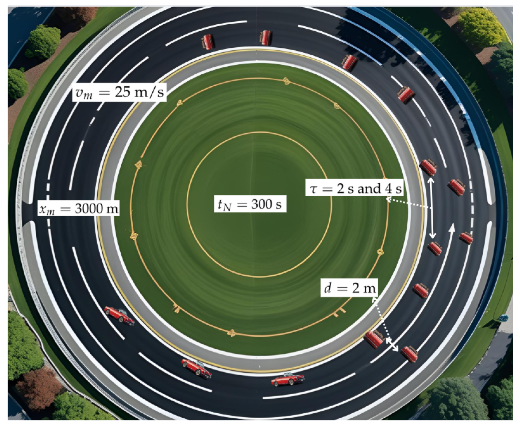
A circular road of length 3000 m is considered with periodic boundary conditions to evaluate the performance of the models. The models are implemented in MATLAB, and the simulation parameters are shown in Figure 2. The road length x_m is divided into M = 300 segments of size δx = 10 m. The time step is δt = 0.1 s, and there are N = 3000 time steps, so the simulation time is t_N = 300 s. To ensure numerical stability, the Courant–Friedrichs–Lewy (CFL) condition [51] is applied [48]. The density $\rho (x,t)$, velocity $v(x,t)$, and driver reaction $P(x,t)={\left({\displaystyle \frac{1}{\tau }}\left({\displaystyle \frac{-88.68}{v_n(0.003d+1.22)}}+80.02\right)\right)}^2\rho (x,t)$ for the proposed model, and reaction time $P(x,t)=C_0^2\rho (x,t)$ for the PW model, are stored in two-dimensional arrays of size M × N. The initial density profile $\rho (x,0)$ has the following distribution:

$$\rho (x,0)=\left\{\begin{array}{cc}0.7,\hfill & x\le 500,\hfill \\ 0.2,\hfill & 500<x\le 1000,\hfill \\ 0.7,\hfill & 1000<x\le 1500,\hfill \\ 0.2,\hfill & 1500<x\le 2000,\hfill \\ 0.7,\hfill & 2000<x\le 2500,\hfill \\ 0.1,\hfill & x\le 3000\hfill \end{array}\right.$$

(33)

The initial velocity is based on the Greenshields equilibrium velocity (3) and is

$$v(x,0)=v_m\left(1-{\displaystyle \frac{\rho (x,0)}{{\rho }_m}}\right),$$

(34)

where v_m = 25 m/s is the free-flow speed and ρ_m = 1 is the maximum normalized density. The initial density is multi-cluster, which can be considered the worst case. The relaxation time is τ = 2 s and 4 s, while the lateral distance headway is d = 2 m, as in [52,53]. The speed constant for the PW model ranges from 2.4 m/s to 57 m/s [54], so here, $C_0=\sqrt{45}$ m/s. The circular road and corresponding simulation parameters are given in Figure 2, and the simulation parameters are summarized in

Table 4. Simulation Parameters.

Parameter	Value
Simulation time	tN = 300 s
Number of road segments	M = 300
Circular road length	xm = 3000 m
Maximum velocity	vm = 25 m/s
Time step	δt = 0.1 s
Road step	δx = 10 m
Relaxation time	τ = 2 s and 4 s
Lateral distance headway	d = 2 m
Velocity distribution	Greenshields (3)
Maximum normalized density	ρm = 1
Speed constant	$C_0=\sqrt{45}$ m/s

.

For time step n, the periodic boundary conditions are employed by updating the initial cells as follows:

$$\begin{array}{cc}\hfill R_1^n& =R_{M+1}^n,R_{M+2}^n=R_2^n,\hfill \\ \hfill V_1^n& =V_{M+1}^n,V_{M+2}^n=V_2^n.\hfill \end{array}$$

Then, the fluxes are computed using (28), (29), (30), and (31), and the conserved variables are updated using (32). Driver reaction for the proposed model is updated as

$$p_i^{n+1}={\left({\displaystyle \frac{1}{\tau }}\left({\displaystyle \frac{-88.68}{v_n(0.003d+1.22)}}+80.02\right)\right)}^2{R}_i^{n+1},$$

(35)

while for the PW model it is

$$p_i^{n+1}=C_0^2{R}_i^{n+1}.$$

(36)

Finally, the arrays for density, velocity, and driver reactions are updated, and the spatial positions are adjusted accordingly.

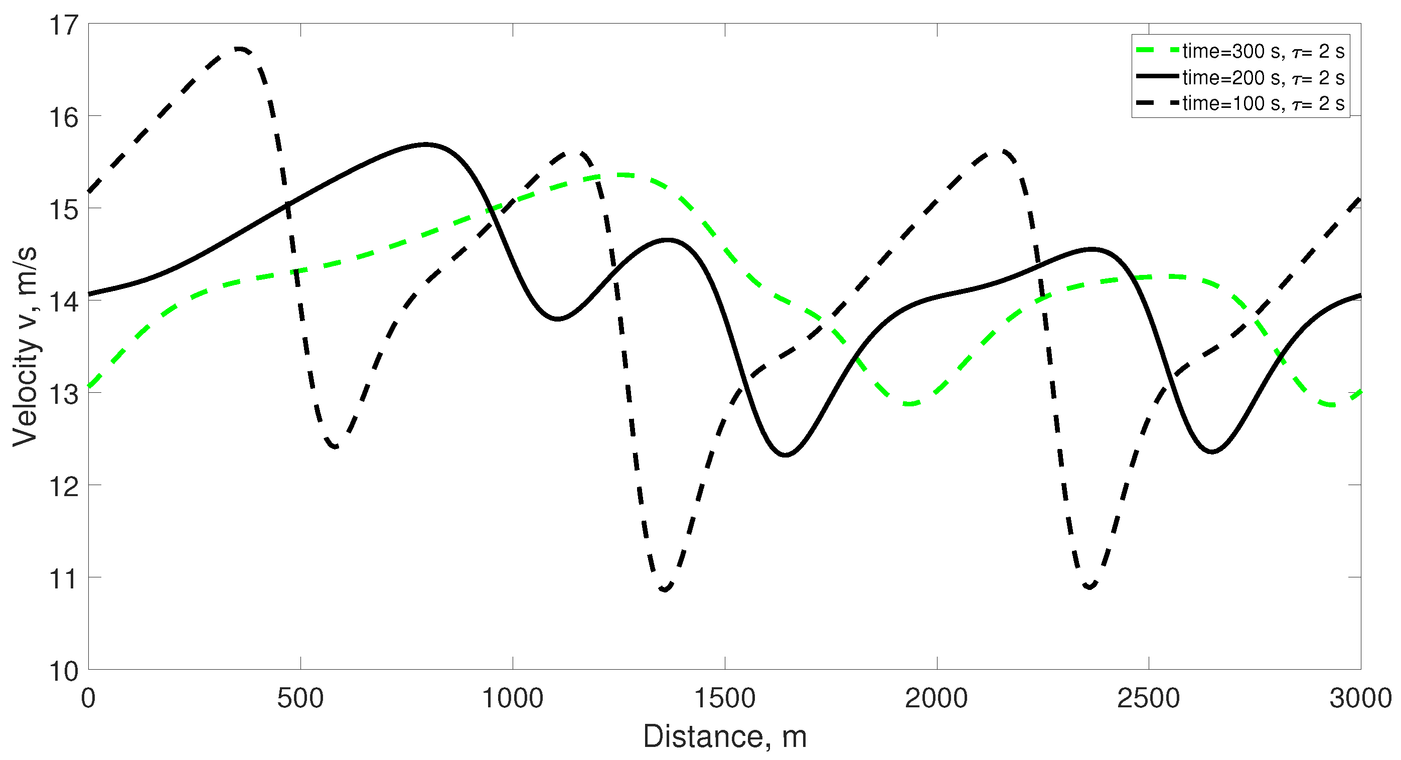
Figure 3 presents the velocity for the proposed model over a 3000 m circular road at 100 s, 200 s, and 300 s. At 100 s, the velocity is 15.2 m/s at 0 m and decreases to 12.5 m/s at 600 m. It is 15.5 m/s at 1250 m and then decreases to 10.8 m/s at 1380 m, which is the lowest value. The velocity then increases to 15.5 m/s at 2300 m. At 200 s, the velocity is 14.1 m/s at 0 m and increases to 15.0 m/s at 600 m. It decreases to 13.8 m/s at 1250 m and then increases to 14.5 m/s at 1380 m. The minimum velocity is 12.5 m/s at 1700 m, and the velocity is 14.4 m/s at 2400 m. At 300 s, the velocity is 13.0 m/s at 0 m and increases to 14.4 m/s at 600 m. It is 15.0 m/s at 1250 m and then decreases to 14.5 m/s at 1380 m and 13.5 m/s at 1700 m. The velocity is 14.2 m/s at 2400 m. These results show that the velocity becomes smoother over time. 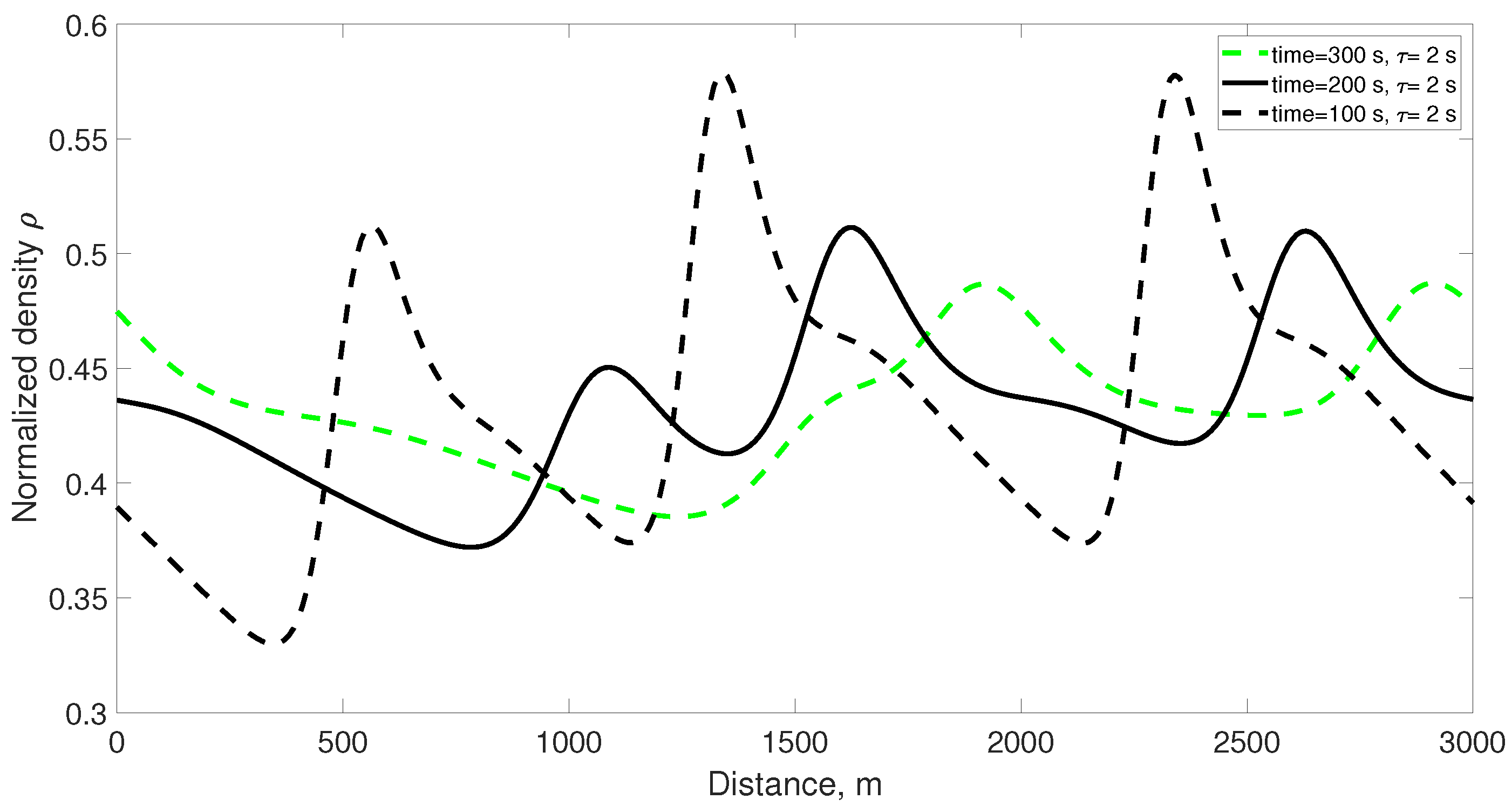Figure 4 presents the corresponding normalized density. At 100 s, the density is 0.39 at 0 m and increases to 0.50 at 600 m. It is 0.46 at 1250 m and 0.57 at 1380 m, with a maximum of 0.58 at 2300 m. At 200 s, the density is 0.44 at 0 m and decreases to 0.41 at 600 m. At 1250 m, it is 0.45, decreases to 0.43 at 1380 m, and then increases to 0.52 at 1700 m. The density is 0.44 at 2400 m. At 300 s, the density is 0.47 at 0 m and decreases to 0.44 at 600 m, 0.40 at 1250 m, and 0.39 at 1380 m. It then increases to 0.45 at 1700 m and 0.48 at 2900 m. As with the velocity, the density becomes smoother over time.

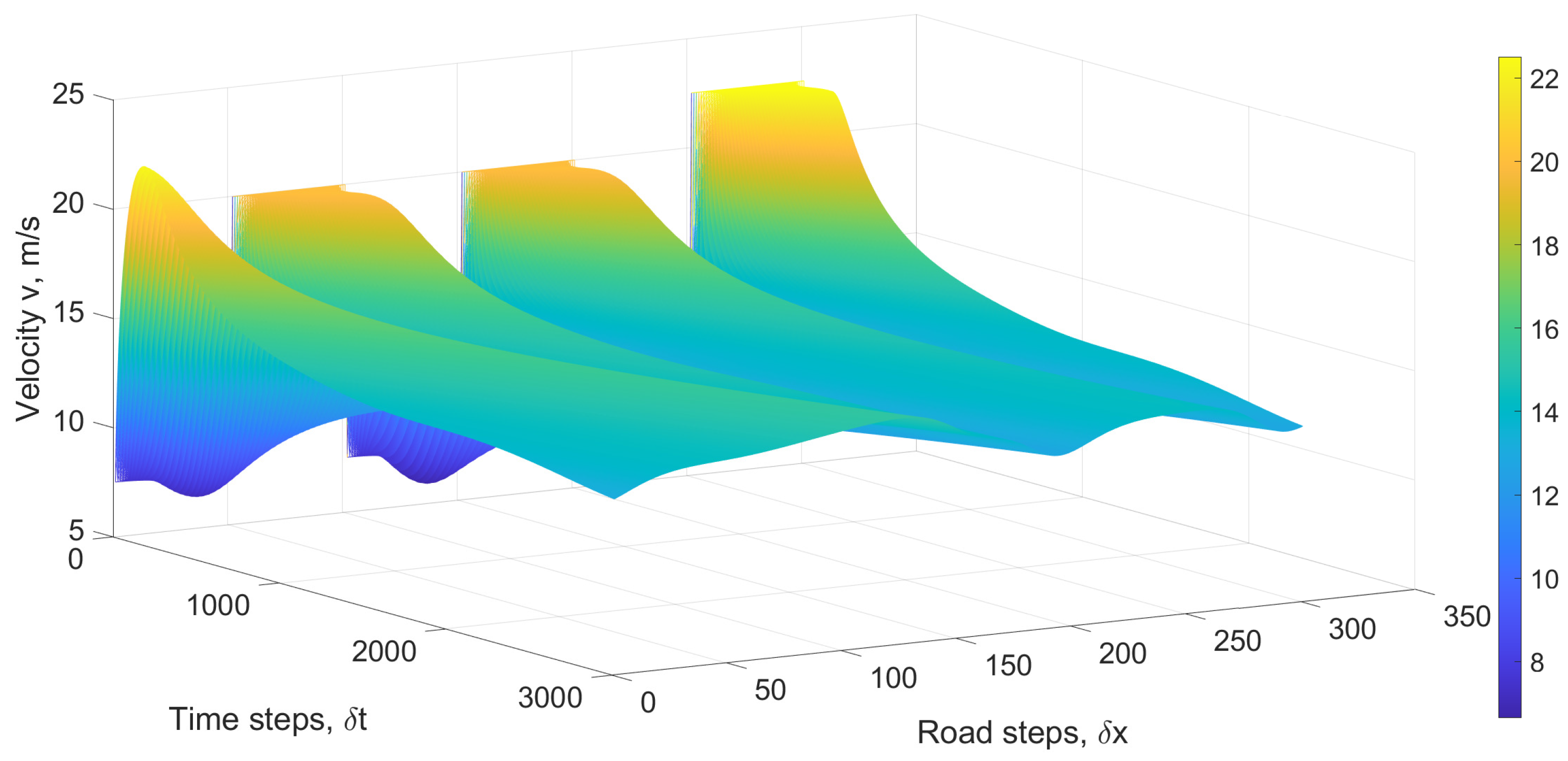
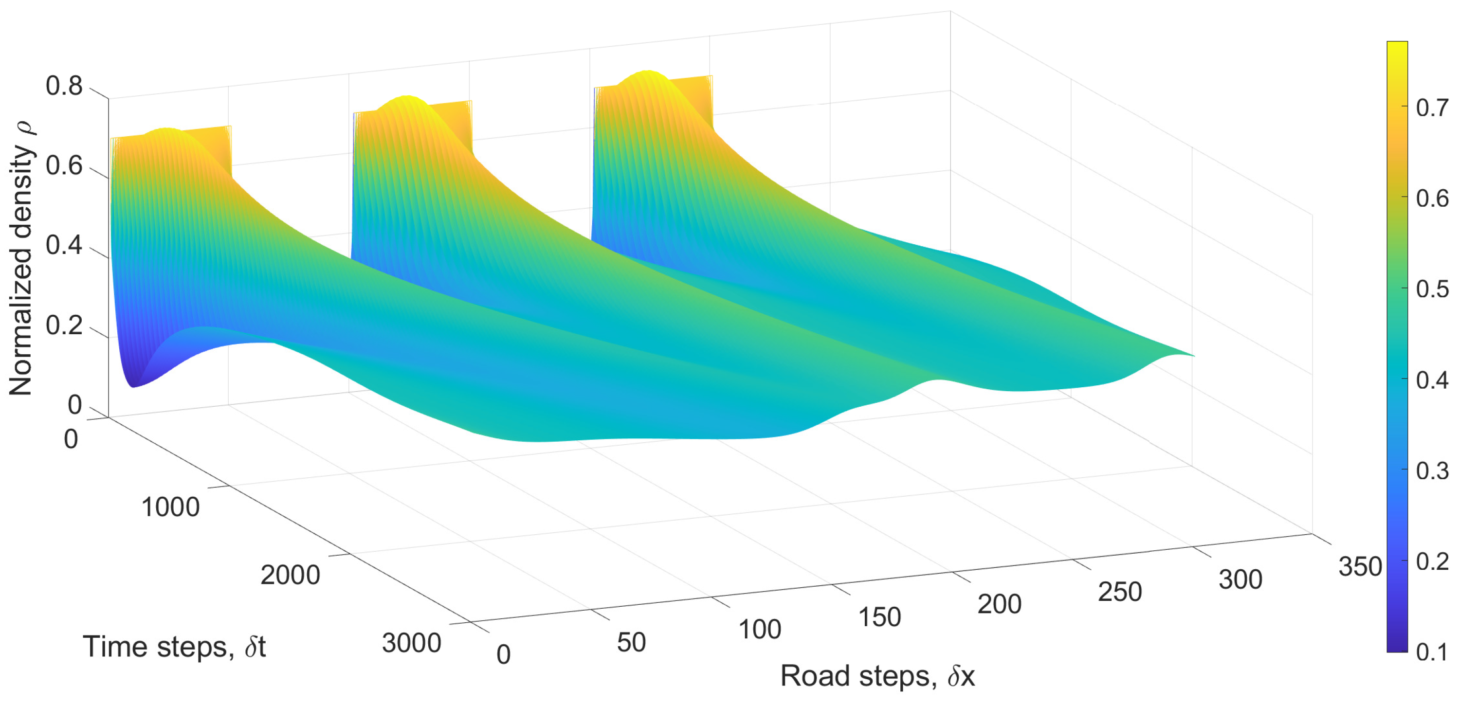
Figure 5 presents the velocity with the proposed model for 300 s over a 3000 m circular road with relaxation time 2 s. The minimum velocity is 0 m/s and the maximum is 25 m/s, and the results remain within these bounds. Initially, there are significant variations due to the multi-cluster density distribution, but over time, they diminish, which reflects realistic traffic evolution. Figure 6 presents the corresponding density. This shows that the density remains within the range 0 to 1, as required. Over time, the density variations decrease and the traffic becomes smooth, as expected.

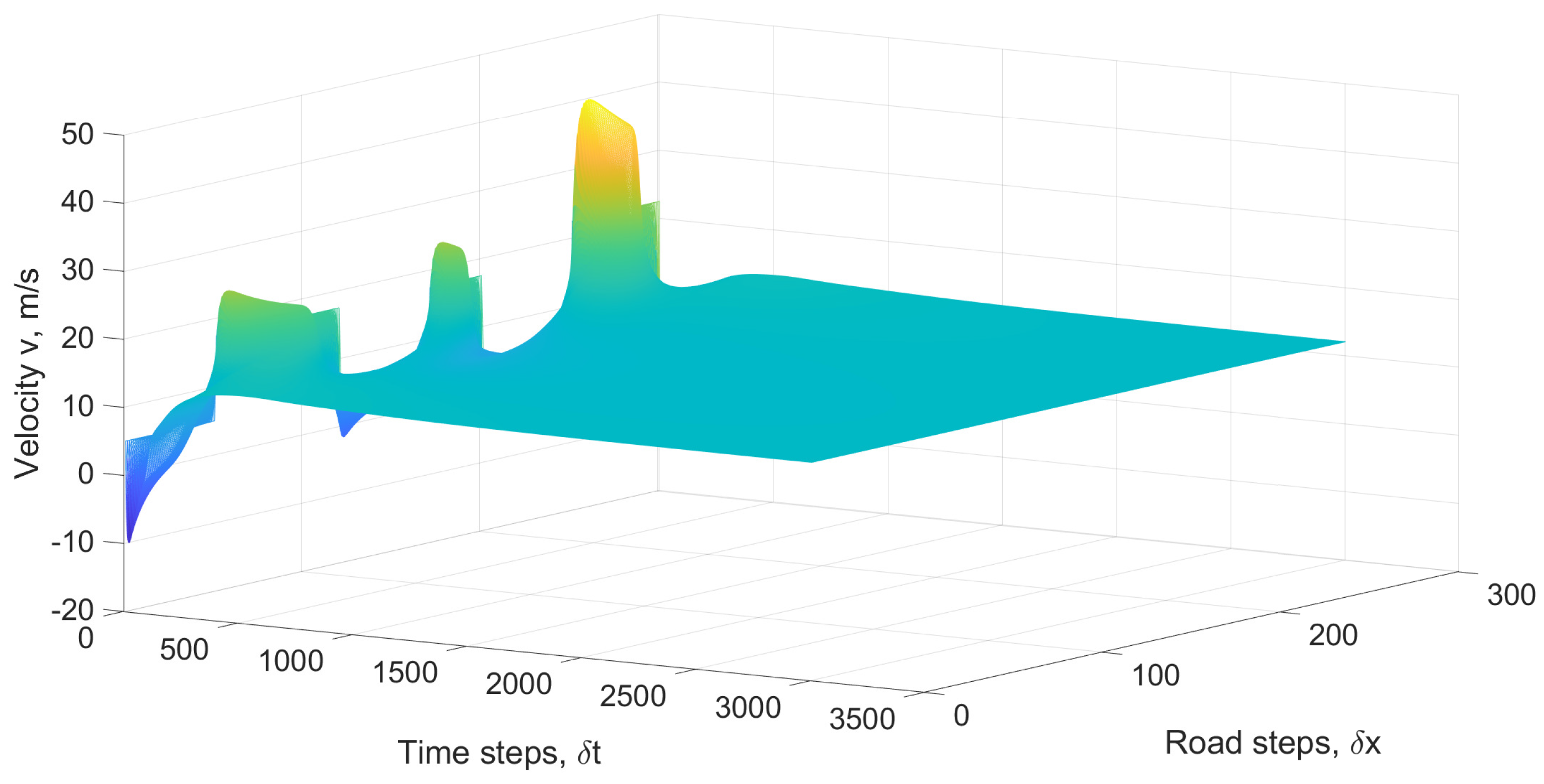
Figure 7 presents the velocity with the proposed model over a 3000 m circular road at 100 s, 200 s, and 300 s. The relaxation time is 4 s and the lateral distance headway is 2 m. At 100 s, the velocity is 15.0 m/s at 0 m and increases to 17.0 m/s at 400 m. There is a peak of 15.0 m/s at 1250 m and then a decrease to the minimum of 8.0 m/s. The velocity is 15.9 m/s at 2300 m. At 200 s, the velocity is 16.1 m/s at 0 m and decreases to 15.0 m/s at 600 m. At 1250 m, it is 13.0 m/s, increases to 14.8 m/s at 1380 m, and then decreases to 7.5 m/s at 1500 m. The velocity is 16.2 m/s at 2400 m. At 300 s, the velocity is 16.4 m/s at 0 m and decreases to 16.1 m/s at 600 m. It is 16.2 m/s at 1250 m, decreases to 6.4 m/s at 1450 m, and then increases to 16.3 m/s at 2300 m. The minimum velocity is 5.0 m/s at 2400 m. These results show that the variations in velocity decrease over time.

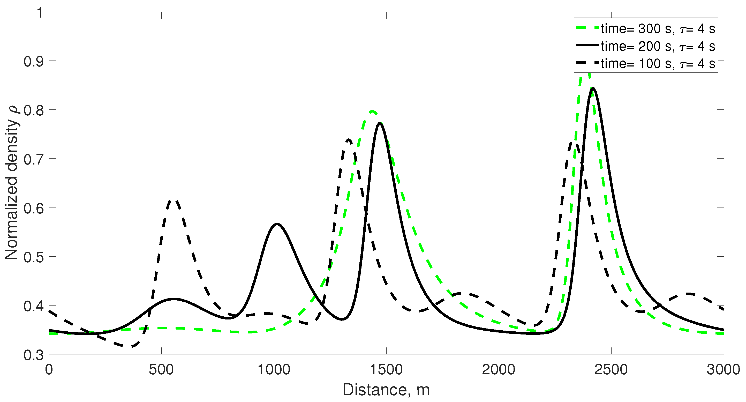
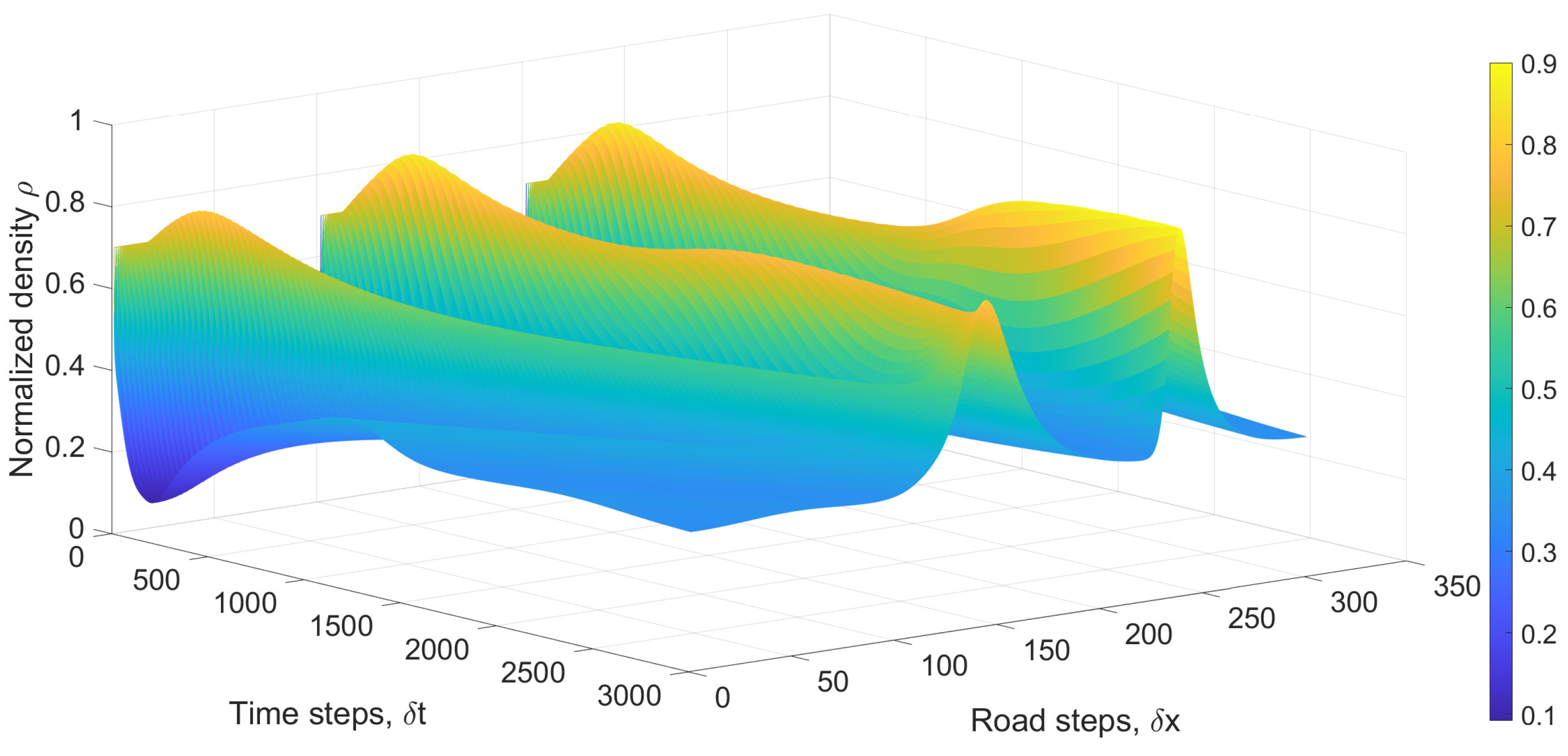
Figure 8 presents the corresponding density. At 100 s, the density is 0.39 at 0 m and decreases to 0.32 at 400 m. It increases to 0.61 at 600 m, decreases to 0.35 at 1250 m, and then increases to 0.72 at 1380 m. The maximum density is 0.71 at 2300 m. At 200 s, the density is 0.35 at 0 m and increases to 0.41 at 600 m. It is 0.58 at 1100 m and decreases to 0.36 at 1380 m. The density is 0.75 at 1550 m and decreases to 0.35 at 2400 m. At 300 s, the density at 0 m is 0.34 and increases to 0.35 at 600 m, 0.77 at 1450 m, and 0.81 at 2450 m. It then decreases to 0.35 at 3000 m. These results show that the maximum density increases over time, and the variations are the least at 100 s.

Figure 9 presents the velocity with the proposed model for 300 s over a 3000 m circular road with relaxation time 4 s. This shows that the velocity remains within the range 0 m/s to 25 m/s, as required. Initially, there are significant variations due to the multi-cluster density distribution, but over time, these variations decrease. Figure 10 presents the corresponding normalized density. The density remains between 0 and 1, as expected, and over time, the variations decrease, consistent with the velocity. Further, a larger relaxation time results in greater variations in velocity and density, as expected.

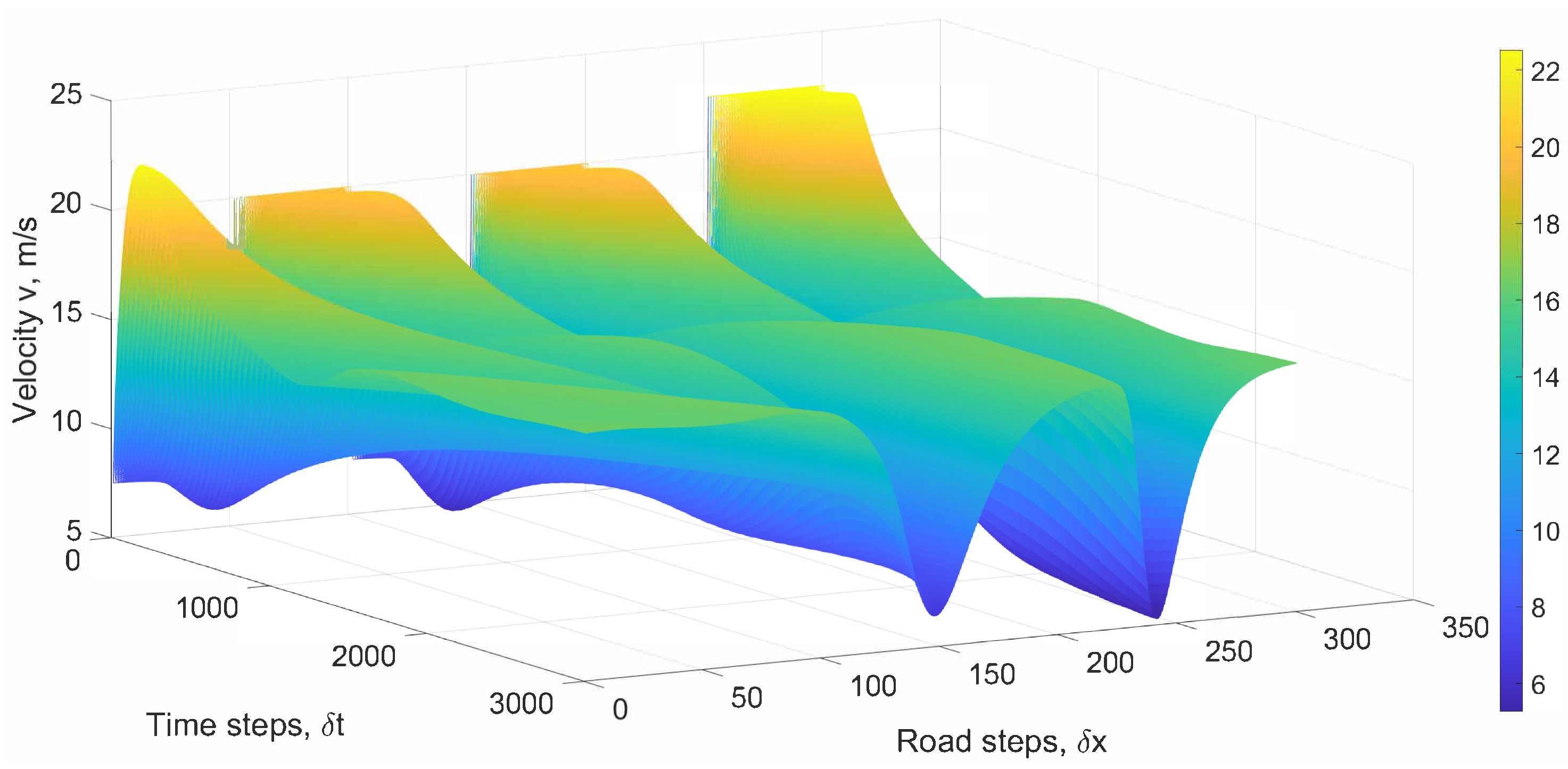
Figure 11 presents the velocity with the PW model over a 3000 m road for 300 s with relaxation time 4 s. This shows that the maximum velocity is 40.8 m/s and the minimum is −11.1 m/s, which exceed the limits of 25 m/s and 0 m/s, respectively. Thus, these results are unrealistic and impossible. The corresponding normalized density is given in Figure 12. Initially, there are large variations in density, but they decrease over time. However, these results are inconsistent with the velocity observed in Figure 11. Therefore, the PW model cannot accurately characterize traffic behavior.

The results above indicate that the variations in traffic behavior with the proposed model are smaller with a shorter relaxation time. In contrast, the PW model produces velocities that exceed the maximum and fall below 0, so the results are unrealistic. Further, t changes in velocity with the PW model do not correspond to the changes in density and so are inconsistent. Conversely, the changes in velocity with the proposed model are in accordance with the changes in density. The velocity is greater with a smaller density, which is consistent with real-world traffic conditions.

Driver Reaction

The proposed model driver reaction is now evaluated for the initial density distribution

$${\rho }_0=\left\{\begin{array}{cc}0.6,\hfill & x\le 500,\hfill \\ 0.1,\hfill & 500<x\le 1000,\hfill \\ 0.6,\hfill & 1000<x\le 1500,\hfill \\ 0.1,\hfill & 1500<x\le 2000,\hfill \\ 0.6,\hfill & 2000<x\le 2500,\hfill \\ 0.1,\hfill & x\le 3000,\hfill \end{array}\right.$$

(37)

and non-periodic boundary conditions. A 3000 m straight road is considered, as shown in Figure 13. The simulation parameters are also given. Figure 14 presents the driver reaction with the proposed model for a lane change with relaxation time 4 s. This shows that driver reaction varies between 2.39 and 0.37 and is large when the density is high. Figure 15 gives the driver reaction for a lane change with relaxation time 2 s. In this case, the driver reaction varies between 8.29 and 1.47, so the range is greater with a smaller relaxation time, and driver reaction for a lane change is higher.

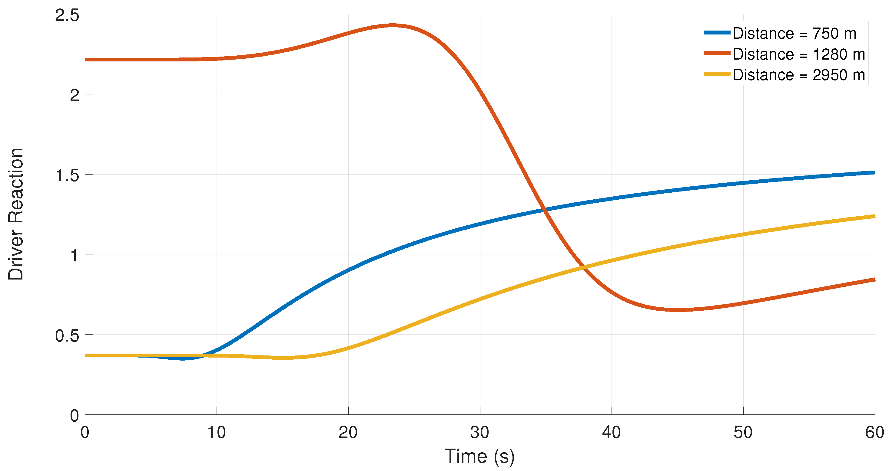
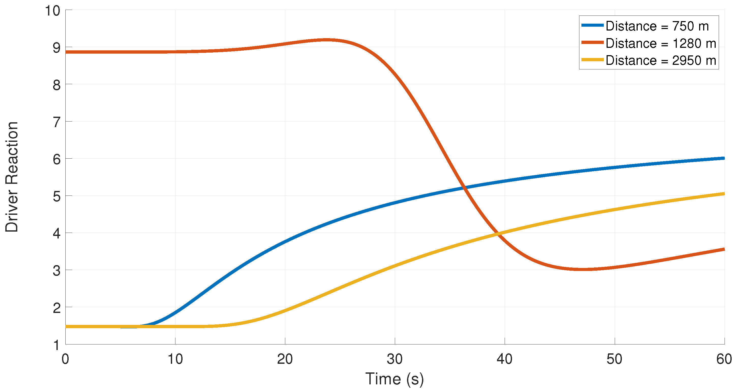
Figure 16 presents the driver reaction for lane changes at 750 m, 1280 m, and 2950 m for 60 s with relaxation time 4 s. At 10 s, the driver reaction is 0.40 at 750 m, 2.22 at 1280 m, and 0.37 at 2950 m. At 30 s, the corresponding values are 1.19, 1.98, and 0.72, respectively. At 50 s, driver reaction increases to 1.44 at 750 m, decreases to 0.70 at 1280 m, and increases to 1.13 at 2950 m. Figure 17 gives the corresponding driver reaction with relaxation time 2 s. At 10 s, the driver reaction is 1.84 at 750 m, 8.87 at 1280 m, and 1.48 at 2950 m. At 30 s, the values increase to 4.82, 8.28, and 3.12, respectively, and at 50 s, they are 5.76 at 750 m, 3.06 at 1280 m, and 4.62 at 2950 m. These results indicate that for multi-cluster traffic, driver reaction varies more with a smaller relaxation time. In addition, driver reaction varies according to the local traffic conditions.

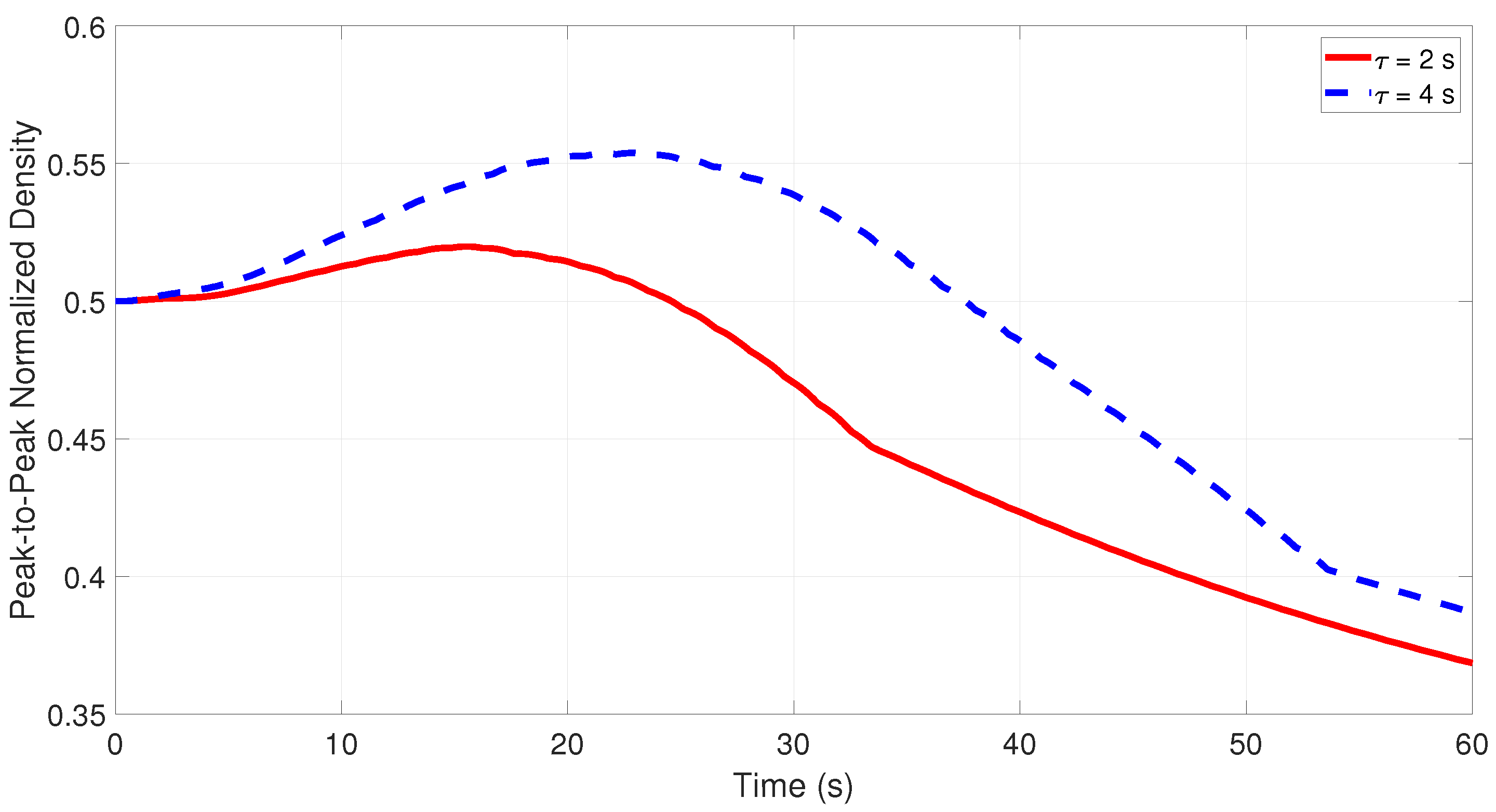
Figure 18 presents the peak-to-peak normalized density on a 3000 m straight road for 60 s with relaxation time 2 s and 4 s. This is the difference between the maximum and minimum density on the road. At 10 s, it is 0.51 with relaxation time 2 s and 0.52 with relaxation time 4 s. At 30 s with relaxation time 2 s it is 0.47, and with relaxation time 4 s, it is 0.54. With relaxation time 4 s the congestion is larger at 30 s, as the density difference has increased. At 50 s, with relaxation time 2 s the density difference is 0.39, while with relaxation time 4 s it is 0.42. Thus, the congestion is dissipating as the difference is decreasing.

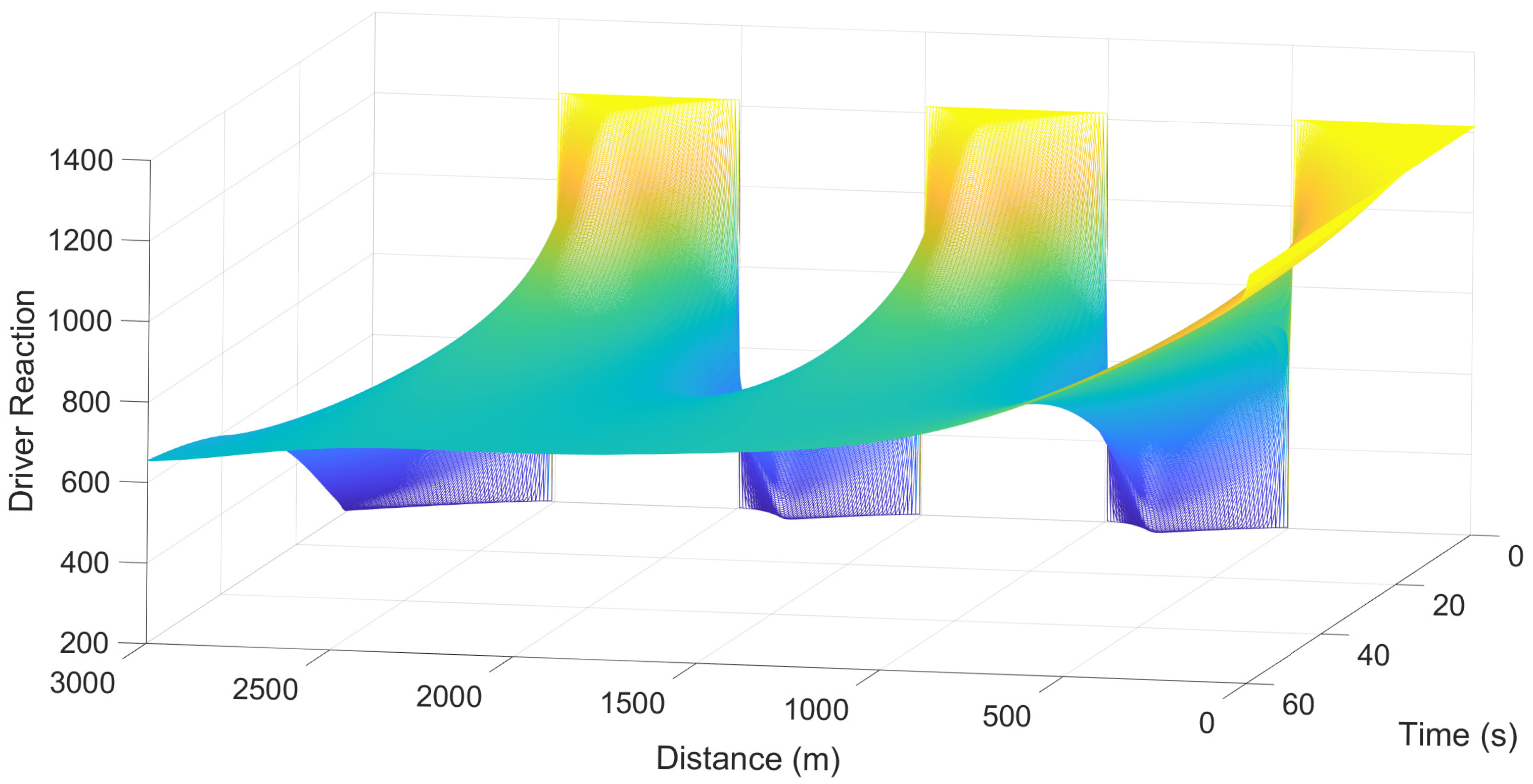
Figure 19 gives the driver reaction with the PW model over a 3000 m straight road for a lane change with relaxation time 2 s and 4 s, and $C_0=\sqrt{45}$. This shows that the driver reaction varies between 1215 and 214 at 1 s. After 60 s, it is between 1215 at 0 m and 654.3 at 3000 m. The corresponding results with relaxation time 4 s are the same, so driver reaction does not vary according to the traffic conditions. 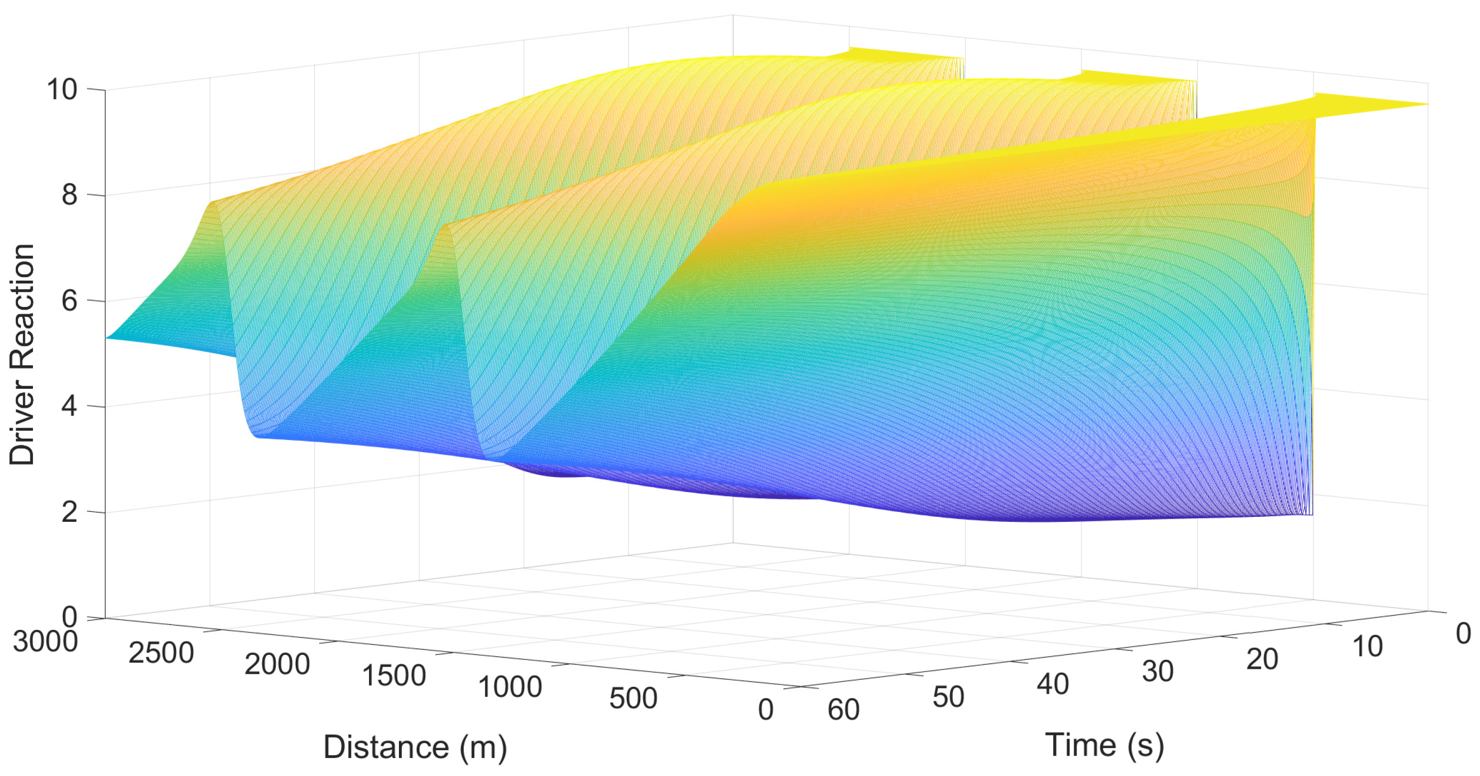Figure 20 gives the corresponding driver reaction with C₀ = 4. The driver reaction varies between 9.60 and 1.60 at 1 s. After 60 s, it is between 3.78 and 8.27. Thus, the variations in driver reaction to a lane change decrease with C₀. However, this is a constant that is not based on traffic physics, so the results are artificial. The driver reaction with the proposed model increases with density and is consistent with the relaxation time. With the PW model, the driver reaction is very large, which is unrealistic, and it does not change with the relaxation time.

8. Conclusions

In this paper, a macroscopic traffic model based on the relaxation time and lateral distance headway was proposed. Models for the lateral time headway and flow were obtained using nonhomogeneous traffic data from Iran and Pakistan, respectively. The use of real-world data provides realistic and accurate models that reflect traffic physics. It was shown that the results with the PW model exceed physical limits, and the traffic behavior does not reflect the changes in density. Further, the velocity evolves similarly for different relaxation times, which is incorrect. Conversely, the variations in density and velocity with the proposed model are greater with a larger relaxation time, and the velocity is consistent with the changes in density. The velocity with the proposed model is within the physical limits. Driver reaction with the proposed model changes according to the relaxation time, whereas with the PW model, it is based on a constant and so is unrealistic. The results presented show that the proposed model can effectively characterize nonhomogeneous traffic under different conditions, unlike the PW model.