Article

An Attention-Enhanced Bivariate AI Model for Joint Prediction of Urban Flood Susceptibility and Inundation Depth

1
School of Civil and Environmental Engineering, University of Ulsan, Ulsan 44610, Republic of Korea
2
Faculty of Civil Engineering, Ho Chi Minh City University of Technology, Ho Chi Minh City 700000, Vietnam
3
Faculty of Civil Engineering, Ho Chi Minh City Open University, Ho Chi Minh City 700000, Vietnam
*
Author to whom correspondence should be addressed.
Mathematics 2025, 13(16), 2617; https://doi.org/10.3390/math13162617
Submission received: 25 June 2025 / Revised: 23 July 2025 / Accepted: 13 August 2025 / Published: 15 August 2025

Abstract

This study presents a novel bivariate-output deep learning framework based on LeNet-5 for the simultaneous prediction of urban flood susceptibility and inundation depth in Seoul, South Korea. Unlike previous studies that relied on single-output models, the proposed approach jointly learns classification and regression targets through a shared feature extraction structure, enhancing consistency and generalization. Among six tested architectures, the Le5SD_CBAM model—integrating a Convolutional Block Attention Module (CBAM)—achieved the best performance, with 83% accuracy, an Area Under the ROC Curve (AUC) of 0.91 for flood susceptibility classification, and a mean absolute error (MAE) of 0.12 m and root mean squared error (RMSE) of 0.18 m for depth estimation. The model’s spatial predictions aligned well with hydrological principles and past flood records, accurately identifying low-lying flood-prone zones and capturing localized inundation patterns influenced by infrastructure and micro-topography. Importantly, it detected spatial mismatches between susceptibility and depth, demonstrating the benefit of joint modeling. Variable importance analysis highlighted elevation as the dominant predictor, while distances to roads, rivers, and drainage systems were also key contributors. In contrast, secondary terrain attributes had limited influence, indicating that urban infrastructure has significantly altered natural flood flow dynamics. Although the model lacks dynamic forcings such as rainfall and upstream inflows, it remains a valuable tool for flood risk mapping in data-scarce settings. The bivariate-output framework improves computational efficiency and internal coherence compared to separate single-task models, supporting its integration into urban flood management and planning systems.

1. Introduction

Urban flooding has become an increasingly critical global concern, driven by rapid urbanization, the growing frequency of extreme weather events, and the intensifying effects of climate change [1]. These events not only disrupt daily urban life and impose severe economic burdens but also test the resilience of urban infrastructure systems. The impacts are especially pronounced in densely populated areas, where the concentration of people and assets significantly elevates the risk of fatalities and structural damage [2,3,4]. Between 2001 and 2018, floods caused 66,078 deaths globally and affected approximately 1.4 billion people, with total economic losses estimated at USD 309.4 billion [5]. With urban populations expected to grow from 55% of the global population in 2018 to 60% by 2030 and 66% by 2050, the frequency and severity of urban flooding are anticipated to rise—particularly in rapidly expanding cities in Asia.
Developing rapid, accurate, and reliable flood prediction and mapping systems is therefore essential for both emergency response and long-term urban planning. However, despite recent advancements in flood modeling, substantial gaps remain between scientific capabilities and operational requirements. Key limitations include computational inefficiency, challenges in data acquisition, and limited model flexibility [6,7]. Early flood modeling efforts primarily relied on physically based hydraulic and hydrodynamic models, including HEC-RAS, MIKE FLOOD, and SWMM. While these models provide detailed simulations grounded in physical laws, their high computational demand renders them less suitable for real-time forecasting and decision support [8,9,10,11,12]. Moreover, they require extensive, high-resolution input data—such as topographic, meteorological, and infrastructure datasets—which are often difficult, costly, and time consuming to obtain in complex urban settings [13,14]. A further limitation of physically based models lies in their reliance on predefined parameterizations for processes that are difficult to represent explicitly. As a result, these models often fail to adequately capture the nonlinear and multifaceted dynamics of urban flooding, thereby introducing considerable uncertainty into evaluation outcomes [15,16,17,18].
To overcome these challenges, data-driven approaches—those based on machine learning (ML) and deep learning (DL)—have gained significant traction. First, Artificial Intelligence (AI) models dramatically reduce computational demands, making near real-time flood forecasting feasible, even in data-rich or high-resolution contexts. ML and DL techniques excel at capturing complex nonlinear relationships between input features and hydrological responses while maintaining high computational efficiency. These approaches have consistently demonstrated superior predictive accuracy and robustness across various flood forecasting scenarios [19,20,21,22]. Second, many ML/DL models are capable of functioning effectively with incomplete or indirect datasets by leveraging proxy variables and learning from spatiotemporal patterns, thereby mitigating the dependence on exhaustive physical input data. Finally, unlike traditional physically based models, which rely on rigid, predefined parameter structures, AI models learn patterns directly from data without prior assumptions, making them well suited to accommodate the heterogeneous and chaotic nature of urban hydrological systems.
Nevertheless, a significant research gap exists in current data-driven flood models: their tendency to treat flood susceptibility classification and inundation depth estimation as independent tasks. Both outputs are inherently interrelated, as they are influenced by shared hydrological, environmental, and infrastructural factors. This fundamental separation ignores these interdependencies and represents a critical limitation that limits the ability to learn mutual relationships between tasks, reducing both predictive accuracy and model interpretability. Furthermore, treating these tasks separately introduces redundancy in model training and fails to capture joint spatial–temporal patterns that are critical for understanding the complex dynamics of urban flooding. As summarized in Table 1, recent CNN-based flood modeling studies overwhelmingly adopt single-task approaches—focusing either on susceptibility mapping (e.g., [23,24]) or on inundation depth prediction (e.g., [25,26])—thus offering only limited insight into the potential of integrated modeling frameworks.
To address these challenges, this study proposes a novel Bivariate AI Model that simultaneously performs flood susceptibility classification and inundation depth regression. The LeNet-5 architecture was selected as the backbone of our framework based on its proven ability to balance accuracy, simplicity, and computational efficiency, particularly under data-constrained conditions. Our input data for flood prediction consist of relatively small spatial patches (23 × 23 × 8), and the availability of labeled flood event samples is somewhat limited. In such scenarios, deeper architectures like ResNet, U-Net, or Swin Transformer—though powerful in large-scale tasks—often entail a large number of trainable parameters, increasing the risk of overfitting and requiring extensive computational resources and hyperparameter tuning [33,34]. In contrast, LeNet-5 is a lightweight CNN well suited for limited data settings and has demonstrated strong generalization capabilities in flood-related applications. Notably, a recent comparative study [35] showed that LeNet outperformed deeper models such as U-Net, ResNet, and VGG16 in flood detection and segmentation tasks using low-resolution input data. Given these considerations and the characteristics of our dataset, LeNet-5 was deemed an appropriate and effective architectural choice for this study.
To further enhance learning efficiency, the model integrates a Convolutional Block Attention Module (CBAM), which improves feature extraction by focusing on critical spatial and channel-wise information. A hard parameter sharing strategy is employed to allow both tasks to learn from shared representations, improving generalization while reducing redundancy and computational overhead. This unified framework enables a more robust and interpretable assessment of urban flood risk, supporting timely and data-efficient decision making.
The primary objectives of this study are threefold: (1) to design and implement specialized bivariate-output convolutional neural network (CNN) models incorporating attention mechanisms for comprehensive urban flood prediction; (2) to quantitatively evaluate and compare the performance of univariate models and the proposed bivariate-output framework across both classification and regression tasks; and (3) to assess the relative importance of environmental and infrastructural variables in determining urban flood susceptibility and inundation depth. The remainder of this paper is structured as follows. Section 2 introduces the study area and describes the datasets used for training and validation. Section 3 outlines the methodological framework, including model architecture and evaluation metrics. Section 4 presents the experimental results, followed by a discussion of key findings in Section 5. Finally, Section 6 concludes the paper with implications for future research and practical applications in urban flood risk management.

2. Study Area and Data

2.1. Study Area

Seoul, the capital of South Korea, is a densely populated metropolitan city with approximately 9.9 million residents and a total area of 605 km2. Located at approximately 37.5° N and 127.0° E (Figure 1), this megacity lies in a basin surrounded by mountains and is bisected by the Han River. The city’s humid continental climate features annual rainfall of 1200–1600 mm, with 65% concentrated during summer monsoons (June–September), which can lead to flooding [36]. Urbanization since the 1970s has transformed Seoul’s hydrological characteristics, dramatically reducing infiltration [37,38] and elevating the flood risk across the city, particularly in low-lying areas next to rivers and streams [39]. Moreover, existing drainage infrastructure—originally designed for 30-year return period rainfall events—is increasingly inadequate in managing the intensifying precipitation [40,41]. Analysis of historical flood data (1987–2017) has identified eight neighborhoods across six districts as recurrent inundation hotspots, primarily in topographic depressions with insufficient drainage [40]. This situation is worsened by the city’s complex infrastructure and high population density, which increase the vulnerability to flood-related damages [41,42,43].
To simplify modeling, we assume that infrastructure, topography, and land cover remain static over the 2010–2024 study period. While this assumption does not fully capture the dynamic nature of urban environments, it is considered reasonable given Seoul’s relatively stable urban development during this time. Nevertheless, we acknowledge that small-scale or localized changes (e.g., new construction or redevelopment) may have introduced minor discrepancies in model predictions. Additionally, we recognize the potential for bias in historical flood records, particularly due to underreporting or inconsistencies in documenting low-severity events. To mitigate the influence of such label uncertainty, we applied data augmentation and cross-validation to enhance the model robustness and generalizability.

2.2. Flood Inundation Inventory

To construct the predictand for the deep learning models, a historical flood event database compiled by the Seoul Metropolitan Government (covering the period from 2010 to 2022; see Table 2 and Figure 1) was utilized. From all reported flood-affected areas across Seoul, a total of 2523 flood-prone locations were selected based on two criteria: (1) inundation area exceeding 500 m2 and (2) flood depth greater than 0.2 m. To ensure practical relevance and comparability with prior research [28,44], these thresholds were adopted to represent spatially persistent and hydrologically meaningful flood events. The selected locations were used to generate localized flood maps for model training. To ensure class balance, an equal number of 2523 non-flooded locations were randomly selected from areas where no inundation was reported [29,45,46]. The final dataset thus comprised 5046 locations, which were randomly split into 70% for training and 30% for testing [24,47]. In addition, K-fold cross-validation (K = 5) was performed on the training set to ensure robust model evaluation and generalization performance.

2.3. Factors Affecting Flood Susceptibility in Urban Environments

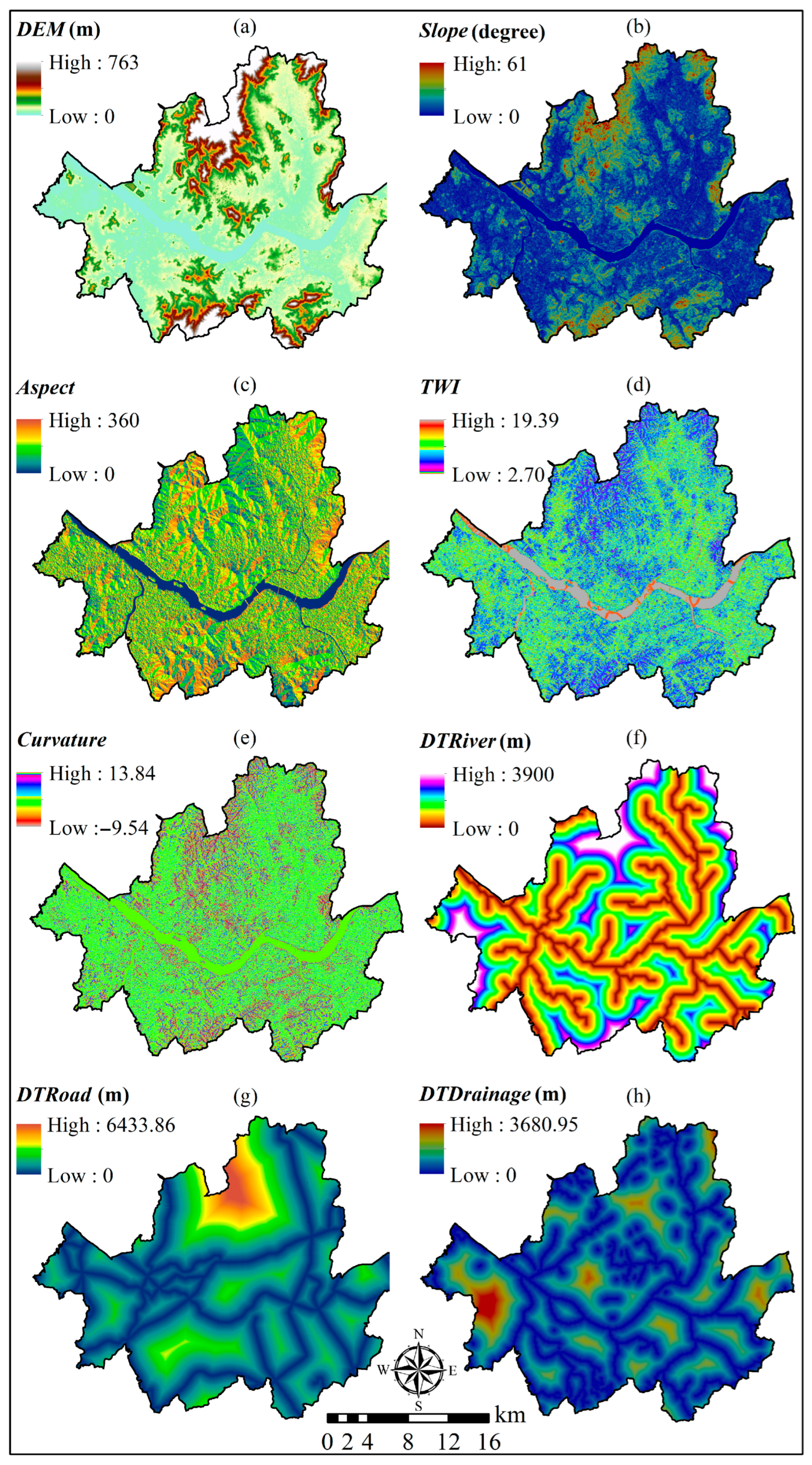
Flood susceptibility in urban environments is shaped by a combination of topographic and infrastructural factors that influence the likelihood and spatial extent of inundation. Based on prior studies [48,49,50] and available geospatial data for the study area, eight key predictors were selected for modeling flood susceptibility and depth: DEM (digital elevation model); slope; aspect (terrain orientation); TWI (topographic wetness index); curvature; DTRiver (distance to river); DTRoad (distance to road); and DTDrainage (distance to stormwater drainage system). These variables represent critical spatial indicators of how terrain and infrastructure influence flood-prone conditions. Detailed descriptions and data sources are summarized in Table 2.
Elevation, derived from a 30 × 30 m resolution DEM, serves as the fundamental terrain representation and plays a pivotal role in runoff accumulation, particularly in low-lying areas [51,52,53,54]. The elevation ranges from 0 m to 760 m, as shown in Figure 2a. Slope (Figure 2b) influences the velocity of surface runoff and the time available for infiltration, thereby affecting the potential for water concentration and accumulation [55]. Aspect (Figure 2c), indicating the orientation of the steepest gradient, reflects directional water movement and can influence microclimatic conditions and runoff pathways [56,57]. The TWI in Figure 2d, a compound topographic indicator calculated as TWI = ln(a/tan β), where a is the upslope contributing area, and β is the local slope angle, is widely used to estimate soil moisture distribution and highlight zones prone to saturation and flooding [58,59]. In the study area, TWI ranged from 2.7 to 19.39, with higher values indicating areas with increased moisture retention. Curvature (Figure 2e) quantifies the concavity or convexity of the terrain surface, where concave regions (negative values) are more likely to accumulate floodwater compared to convex or flat areas [27,60]. Infrastructural proximity factors were also considered, including the Euclidean distance to the nearest river (DTRiver), which reflects potential flood exposure from fluvial overflow [61]; distance to the nearest road (DTRoad), as roads can act as preferential pathways for runoff during heavy rainfall events [62,63]; and distance to the nearest stormwater drainage inlet (DTDrainage), a critical factor in urban areas where drainage systems may become overwhelmed during intense precipitation events, resulting in surface flooding [27]. Together, these predictors provide a comprehensive spatial representation of both natural and built-environmental influences on urban flood susceptibility and depth.
Data augmentation was applied using horizontal flipping and rotation to increase sample diversity while preserving critical local spatial relationships in the 23 × 23 × 8 geospatial input. These transformations were carefully selected to minimize distortion of direction-dependent features such as slope and drainage patterns. In contrast, noise injection was not considered appropriate for this study, as it may introduce inconsistencies in geospatial characteristics and showed only limited potential benefit. The adopted augmentation strategy increased the training data size by approximately threefold and contributed to improved model robustness under limited data conditions. All input features were normalized using Min–Max normalization to a [0, 1] range. This method was chosen to preserve spatial relationships, which is essential in geospatial modeling. The input variables used in this study (e.g., elevation, distance to roads, topographic indices) exhibit skewed and bounded distributions, for which z-score normalization is less suitable. Min–Max scaling prevents any single feature from dominating others during training and is consistent with established practices in urban flood modeling [26,27,30], thereby improving comparability and reproducibility.

3. Methodology

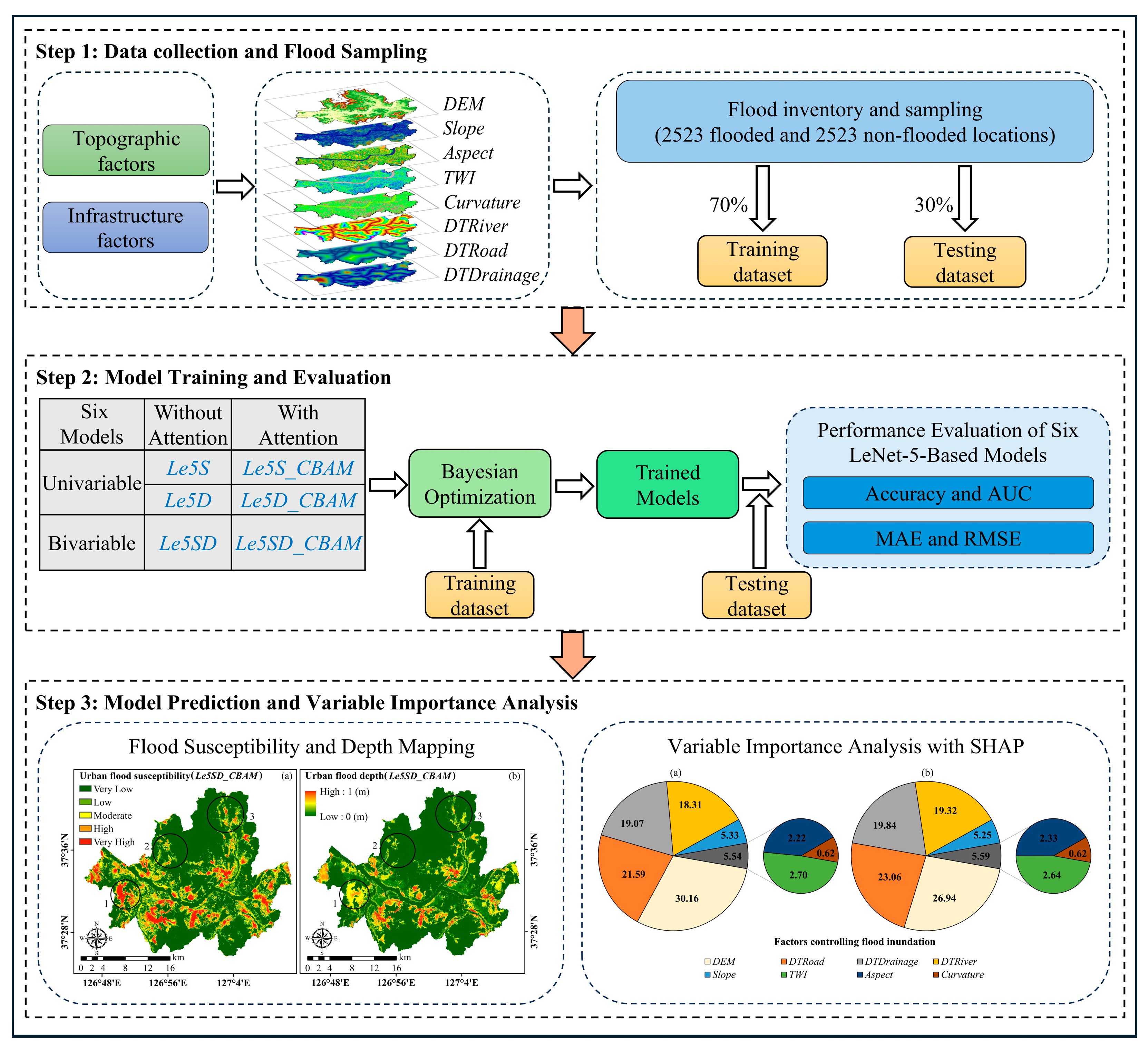
The proposed framework follows a three-step process (Figure 3). First, a comprehensive dataset is constructed by integrating topographic and infrastructural variables with historical inundation hotspot data. The dataset is then partitioned into 70% for training and 30% for testing. Second, six deep learning models based on the LeNet-5 architecture with (and without) attention mechanism are developed, trained, and optimized through Bayesian optimization, with performance evaluated using Accuracy, Area Under the ROC Curve (AUC), mean absolute error (MAE), and root mean squared error (RMSE). In the final step, the best-performing model is used to generate spatial maps of flood susceptibility and depth. Furthermore, SHapley Additive exPlanations (SHAP) is applied to quantify the contribution of each predictor variable, thereby improving model interpretability and offering insights into key environmental and infrastructural drivers of urban flooding.

3.1. Univariate- and Bivariate-Output AI Models

Convolutional Neural Networks (CNNs) have emerged as one of the most prominent deep learning architectures for spatial data analysis, particularly in image recognition and classification tasks. Representative CNN models include AlexNet, VGGNet, ResNet, and Inception, each offering varying depths and feature extraction capacities. While these models are commonly used in computer vision, their application in geospatial and environmental modeling has grown substantially due to their ability to capture spatial hierarchies and local patterns from gridded input data. In the context of urban flood prediction, CNNs are particularly advantageous because flood-related variables—such as topography, infrastructure layout, and proximity metrics—are inherently spatial and can be effectively encoded as rasterized input layers. This spatial structure makes CNNs more suitable than recurrent neural networks (RNNs), which are designed for temporal sequence modeling. Although RNNs and their variants like LSTM are effective in time series forecasting (e.g., rainfall—runoff prediction), they are less optimal when the primary focus is on learning spatial dependencies from static or quasi-static input maps. Given that our study aims to simultaneously classify flood susceptibility and estimate flood depth using spatially distributed variables, CNN-based architectures offer a better fit.
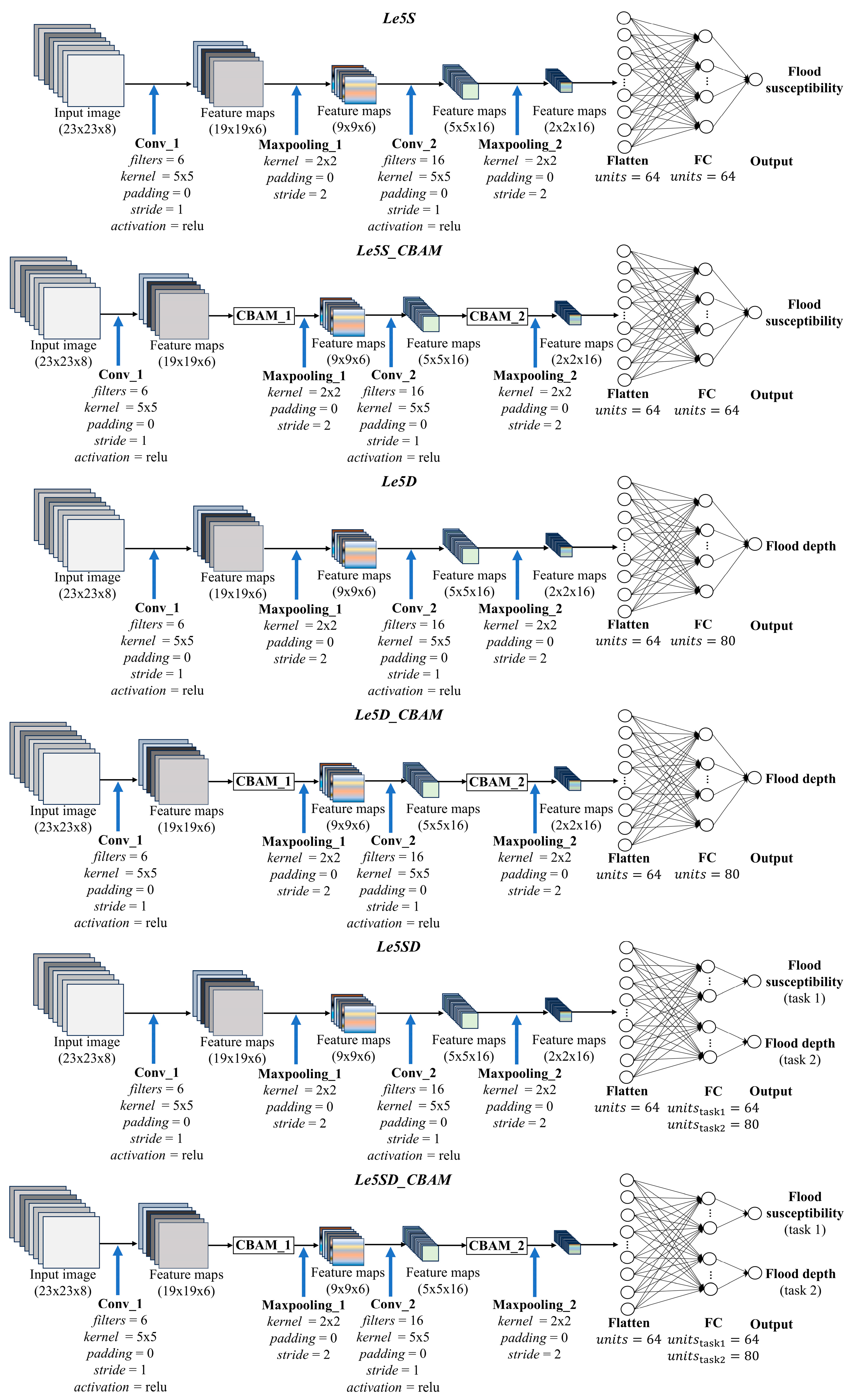
Among the many CNN options, LeNet-5 was selected as the backbone architecture for its simplicity, computational efficiency, and proven performance in spatial classification tasks. LeNet-5 is one of the earliest CNN architectures and, despite its relatively shallow depth, remains highly effective for structured input data with limited resolution, such as 2D gridded maps commonly used in urban hydrology [27,49]. Its architecture enables fast training and convergence, making it ideal for exploring architectural variations and conducting model interpretability analyses. In this study, we develop six CNN variants based on LeNet-5 to address different urban flood prediction tasks (Figure 4). These include Le5S and Le5S_CBAM (which incorporate a Convolutional Block Attention Module for channel and spatial focus) for flood susceptibility classification; Le5D and Le5SD_CBAM for flood depth regression; and two bivariate-output models—Le5SD and Le5SD_CBAM—that simultaneously perform both tasks through shared feature extraction layers. The use of shared representation across tasks not only reduces redundancy but also leverages the interdependency between susceptibility and depth for enhanced predictive performance.
The adapted LeNet-5 architecture in this study processes input images with a spatial resolution of 23 × 23 pixels, following prior urban flood modeling studies [27,49]. The convolutional (Conv) layers extract spatial features by applying kernels that slide over the input image, performing element-wise multiplication and summation to produce feature maps. The output dimensions of these feature maps are determined by three key parameters: kernel size ( K ), padding ( P ), and stride ( S ). Padding refers to the number of pixels (typically zeros) added around the input to preserve spatial dimensions, while stride controls the step size at which the kernel moves across the input matrix. The spatial dimension d of the output feature map is calculated as follows:
d = I   K   +   2 P S + 1
where I is the input height or width, K is the kernel size, P is the padding, and S is the stride. Max Pooling layers are used to reduce the spatial resolution of feature maps by selecting the maximum value from each local region. This downsampling helps decrease the number of trainable parameters and the computational cost while preserving the most salient features. To mitigate overfitting, a dropout mechanism is applied to the fully connected (FC) layers during training. The final dense layer combines the FC and output layers and performs a weighted sum of inputs, followed by an activation function, to generate the final predictions:
g = f ( W h   +   b )
where h is the input vector; W is a weight matrix; b is a bias vector; and f (z) is the activation function, with z   =   W h   +   b . This study used the Rectified Linear Unit (relu) and the sigmoid functions as the activation functions.
Notably, the bivariate-output models (Le5SD and Le5SD_CBAM) use hard parameter sharing. Initial convolutional blocks (Conv_1 and Conv_2) form the shared backbone. Max Pooling operations also contribute to this shared structure. This approach enables efficient feature extraction for both tasks. This shared representation is then bifurcated after the flattening layer into two task-specific branches: one FC layer with 64 units dedicated to flood susceptibility classification and another FC layer with 80 units for flood depth regression. This architecture promotes the learning of generalized features beneficial to both tasks, serving as an implicit regularization mechanism that mitigates overfitting and substantially reduces the total number of trainable parameters.
During training, binary cross-entropy (BCE) was used for the flood susceptibility classification task, while MAE was adopted for the flood depth regression task. To balance the contributions of the two tasks during training and optimization and to provide flexibility for adjusting their relative importance, we applied task-specific loss weights to each objective. In this study, equal weights were assigned to both tasks to ensure balanced contributions to the shared optimization process.
L = Ψ s × B C E + Ψ d × M A E
B C E = 1 n i = 1 n y i log y i ^ + 1 y i log 1 y i ^
MAE = 1 n i = 1 n η i η ^ i
where L is the loss function of the bivariate-learning framework. Ψ s and Ψ d are the loss weights for the susceptibility classification and flood depth regression tasks, respectively. n denotes the number of samples in the flood inventory. y i is the true label (flood or non-flood) of the i -th sample, and y i ^ is the predicted probability for that sample. η i and η ^ i denote the observed and predicted flood depths of the i -th sample, respectively.

3.2. Convolutional Block Attention Module

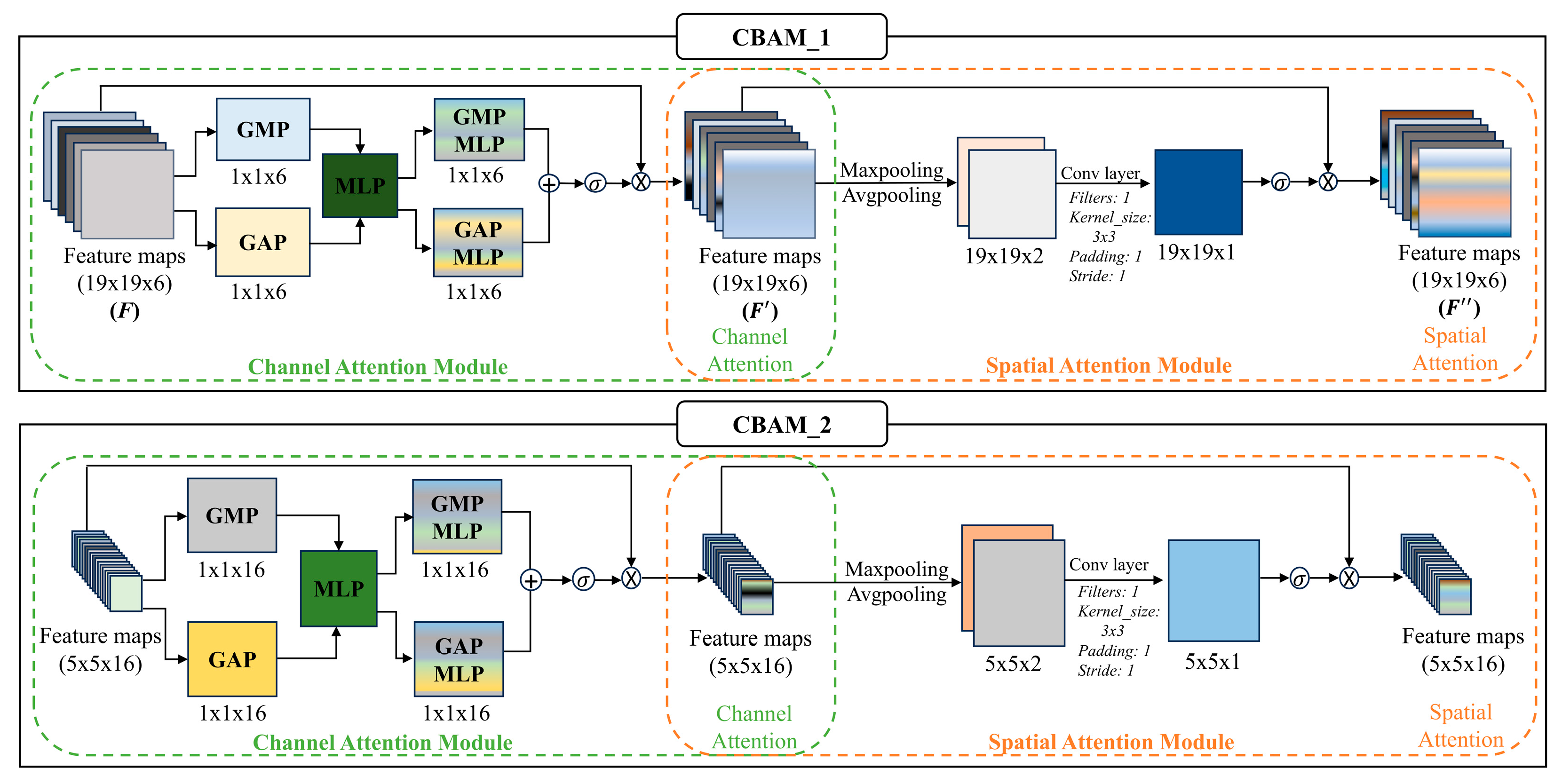
The Convolutional Block Attention Module (CBAM) [64] is an effective attention mechanism specifically designed for convolutional neural networks, operating along both channel and spatial dimensions. Its lightweight and modular design allows seamless integration into existing CNN architectures, supporting end-to-end training without significant computational overhead. In this study, CBAM is embedded at multiple levels within the Le5S_CBAM, Le5D_CBAM, and Le5SD_CBAM models to enhance the quality of feature representations at varying levels of abstraction. As illustrated in Figure 5, the initial feature maps generated by Conv_1 (with dimensions 19 × 19 × 6) are refined via CBAM_1. Additional CBAM modules (CBAM_2) are subsequently applied to deeper layers of the network to further enhance feature maps with dimensions 9 × 9 × 6, 5 × 5 × 16, and 2 × 2 × 16.
CBAM contains two sequential modules. The first is the Channel Attention Module. The second is the Spatial Attention Module. The Channel Attention Module applies Global Max Pooling and Global Average Pooling to input feature map F . This captures complementary information about channel activation patterns. These pooled descriptors are then passed through shared-weight Multi-Layer Perceptrons (MLPs) with a bottleneck (reduction–expansion) structure to model nonlinear channel interdependencies. The outputs are combined and passed through a sigmoid activation function to generate the final channel attention weights, as defined by the following equation:
A ( c ) = σ ( M L P ( G M P ( F ) ) + M L P ( G A P ( F ) ) )
where σ represents the sigmoid activation function that normalizes attention values between 0 and 1. Once these channel-specific weights are determined, they are applied to the original input feature map through element-wise multiplication, producing the channel-refined feature map:
F = A ( c ) F
Next, the Spatial Attention Module is applied to the channel–refined feature map F to identify the most informative spatial regions within the representation. This module begins by generating two spatial context descriptors, using Max Pooling and Average Pooling operations along the channel axis. These complementary representations are concatenated and processed through a convolutional layer with sigmoid activation, generating the spatial attention weights:
A ( s ) = σ ( C o n v 3 × 3 ( [ M a x P o o l ( F ) ; A v g P o o l ( F ) ] ) )
These weights highlight important spatial regions in the feature map, which are then applied to the channel-refined feature map through element-wise multiplication:
F = A ( s ) F
This process yields a refined feature representation in which both channel-wise importance and spatial relevance are effectively emphasized. By allowing the network to simultaneously learn what features are most informative and where they are located within the input, CBAM substantially enhances the model’s capacity to capture critical flood-related patterns. This dual-attention refinement contributes to improved predictive performance, particularly in complex urban flood scenarios where spatial heterogeneity and multiscale features play a crucial role.

3.3. Bayesian Optimization

Bayesian Optimization, a probabilistic model-based optimization technique, was employed to systematically optimize hyperparameters across all models. These hyperparameters include learning rate, dropout rate, batch size, number of training epochs, and the task-specific loss function weights used in the bivariate-learning framework. The method approximates the true objective function using a surrogate probabilistic model—typically a Gaussian Process (GP)—and iteratively selects hyperparameter configurations by maximizing an acquisition function, thereby efficiently balancing exploration and exploitation to identify optimal model settings with minimal computational cost:
x * = a r g m a x x X   α x D
where x represents a candidate set of hyperparameters within the search space X , and x * is the optimal set of hyperparameters chosen to maximize the acquisition function α x D , which adaptively balances exploration and exploitation based on the current observations D . Compared to traditional methods such as grid search or random search, Bayesian optimization offers superior accuracy and significantly enhanced computational efficiency [65]. To implement this process, a customized hyperparameter search space was defined using the Keras Tuner library. The learning rate was explored over a logarithmic scale of [0.0001, 0.001, 0.01], while dropout rates were set to discrete values of [0.2, 0.3, 0.4, 0.5]. Batch sizes were tested at [16,32,48,64], and the number of training epochs ranged from 30 to 100. The number of units in the fully connected layers was varied from 16 to 128. A total of 1000 trials were performed to ensure a comprehensive exploration of the search space. Early stopping with a patience value of 50 was employed to prevent overfitting and improve training efficiency, following established practices in previous studies [66,67,68,69]. The final optimized hyperparameters for each model are summarized in Table 3.

3.4. Performance Evaluation

In this study, four key performance metrics—Accuracy, AUC, MAE, and RMSE—were employed to systematically evaluate the performance of both classification and regression tasks. “Accuracy” is a widely used and fundamental performance metric in machine learning, particularly in binary classification tasks, where it serves as one of the most basic and intuitive indicators of model performance. Accuracy measures the proportion of correctly classified instances relative to the total number of predictions and is calculated as:
Accuracy = T P + T N T P + T N + F P + F N
where True Positives ( T P ) and True Negatives ( T N ) represent correctly identified flooded and non-flooded areas, respectively, while False Positives ( F P ) and False Negatives ( F N ) indicate misclassifications. Of particular concern in flood susceptibility modeling is F N , as it reflects the underestimation of flood-prone areas, posing direct risks to safety and infrastructure.
To assess the model’s ability to discriminate between flooded and non-flooded classes, AUC is used. Higher AUC values indicate better classification performance. Following Yesilnacar (2005) [70], AUC values are generally interpreted as follows: poor (0.5–0.6), fair (0.6–0.7), good (0.7–0.8), very good (0.8–0.9), and excellent (0.9–1.0).
For regression tasks such as flood depth estimation, MAE and RMSE offer complementary insights into prediction accuracy. MAE calculates the average magnitude of absolute errors between predicted ( η ^ i ) and observed ( η i ) flood depths following Equation (5). In contrast, RMSE emphasizes larger errors by incorporating the squared differences between predicted and observed values:
RMSE = 1 n i = 1 n η i η ^ i 2
By combining these four metrics, a multidimensional and rigorous assessment of model performance is achieved, ensuring robust evaluation of both flood classification and depth estimation capabilities.

3.5. Importance of Predictor Variables

The relative importance of predictor variables in machine learning models can be effectively assessed using contribution-based interpretability techniques [71]. In this study, variable importance was quantified using SHapley Additive exPlanations (SHAP), a method introduced by Lundberg and Lee (2017) [72]. SHAP is grounded in Shapley value theory from cooperative game theory, which ensures a fair and theoretically consistent distribution of each feature’s contribution to the model output. The method evaluates a feature’s marginal contribution by averaging its effects across all possible feature subsets, thereby yielding a robust and interpretable metric for feature importance. For more detailed information on the methodology and theoretical foundations of the SHAP algorithm, readers are encouraged to refer to the original publication by Lundberg and Lee (2017) [72].

4. Results

4.1. Model Performance Evaluation

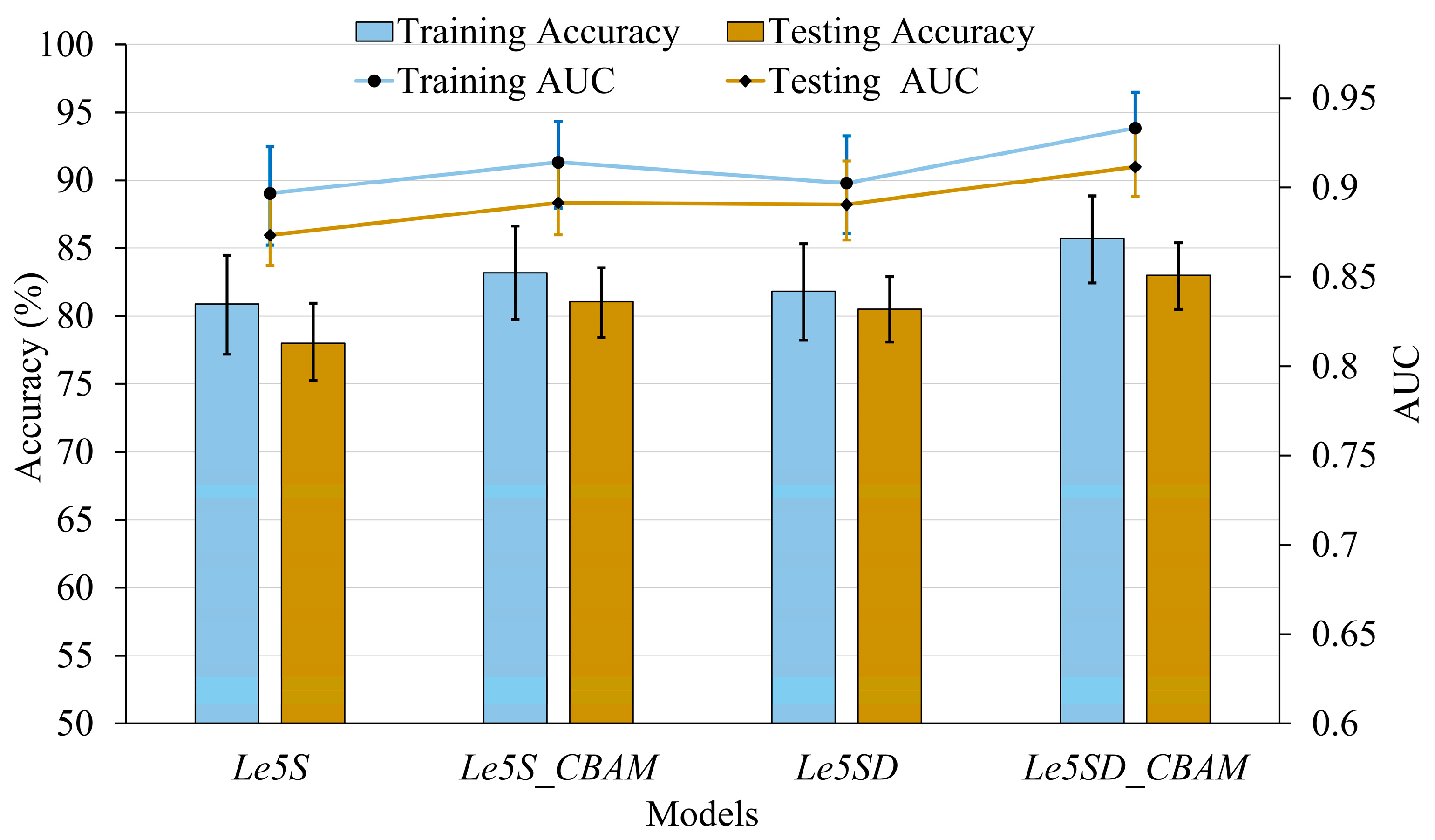
The classification and regression performance of all candidate models were evaluated using both training and testing datasets. For classification, Accuracy and AUC were used to assess model capability (Figure 6). Among the four models (Le5S, Le5S_CBAM, Le5SD, and Le5SD_CBAM), the Le5SD_CBAM model achieved the highest training accuracy (85.74%) and AUC (0.93), demonstrating strong learning capacity. The single-task model Le5S_CBAM also outperformed its baseline counterpart, Le5S, with improvements in both accuracy (83.18% vs. 80.88%) and AUC (0.91 vs. 0.89), confirming the beneficial effect of CBAM. Similarly, in the multitask setting, Le5SD_CBAM surpassed Le5SD in both metrics (accuracy: 85.74% vs. 81.83%; AUC: 0.93 vs. 0.90), reinforcing the value of attention mechanisms in enhancing discriminative power. On the testing set, Le5SD_CBAM again achieved the best classification results (accuracy: 83%, AUC: 0.91), outperforming all other models, including Le5S_CBAM (81.05%, 0.89) and Le5S (78.01%, 0.87). The Le5SD model without attention showed the weakest performance (80.52%, 0.89), highlighting the advantage of integrating CBAM across different model complexities for improved generalization.
For regression, model performance was measured using MAE and RMSE (Figure 7). In the training phase, Le5SD_CBAM showed the lowest MAE (0.12 m) and RMSE (0.17 m), indicating superior accuracy in predicting flood depth. The single-task model Le5D_CBAM also outperformed Le5D (MAE: 0.12 m vs. 0.13 m; RMSE: 0.18 m vs. 0.18 m), again demonstrating the benefit of attention integration. In the testing phase, Le5SD_CBAM maintained the best performance, with an MAE of 0.12 m and RMSE of 0.18 m. While Le5D_CBAM showed slight improvements over Le5D (MAE: 0.13 m vs. 0.13 m; RMSE: 0.18 m vs. 0.19 m), the non-attention multitask model Le5SD had the highest error (MAE: 0.14 m, RMSE: 0.20 m), further emphasizing the importance of attention modules in multitask learning. Across all models, testing errors were consistently 2–4% higher than training errors, suggesting good generalization and no significant overfitting. Overall, CBAM models exhibited not only enhanced predictive accuracy but also more stable and consistent performance across tasks. Based on these results, Le5SD_CBAM was selected as the optimal model for further flood susceptibility mapping, depth estimation, and input variable analysis.
The baseline models (Le5S and Le5D) required approximately 37–57 s for training, with fast inference times around 0.09 s. Incorporating the CBAM module increased training time (e.g., from 37 s for Le5D to 100 s for Le5D_CBAM), reflecting a ~170% increase. However, inference times remained efficient (≤0.21 s), and all CBAM-equipped models completed training in under 2 min. Furthermore, the proposed multitask model (Le5SD_CBAM) reduced the total training time and parameter count compared to training two single-task models separately, while maintaining or improving predictive performance. As summarized in Table 4, these results demonstrate that the additional computational cost introduced by CBAM and the multitask framework is modest and practically negligible, making the model suitable for real-world urban flood forecasting applications.

4.2. Flood Susceptibility and Depth Mapping

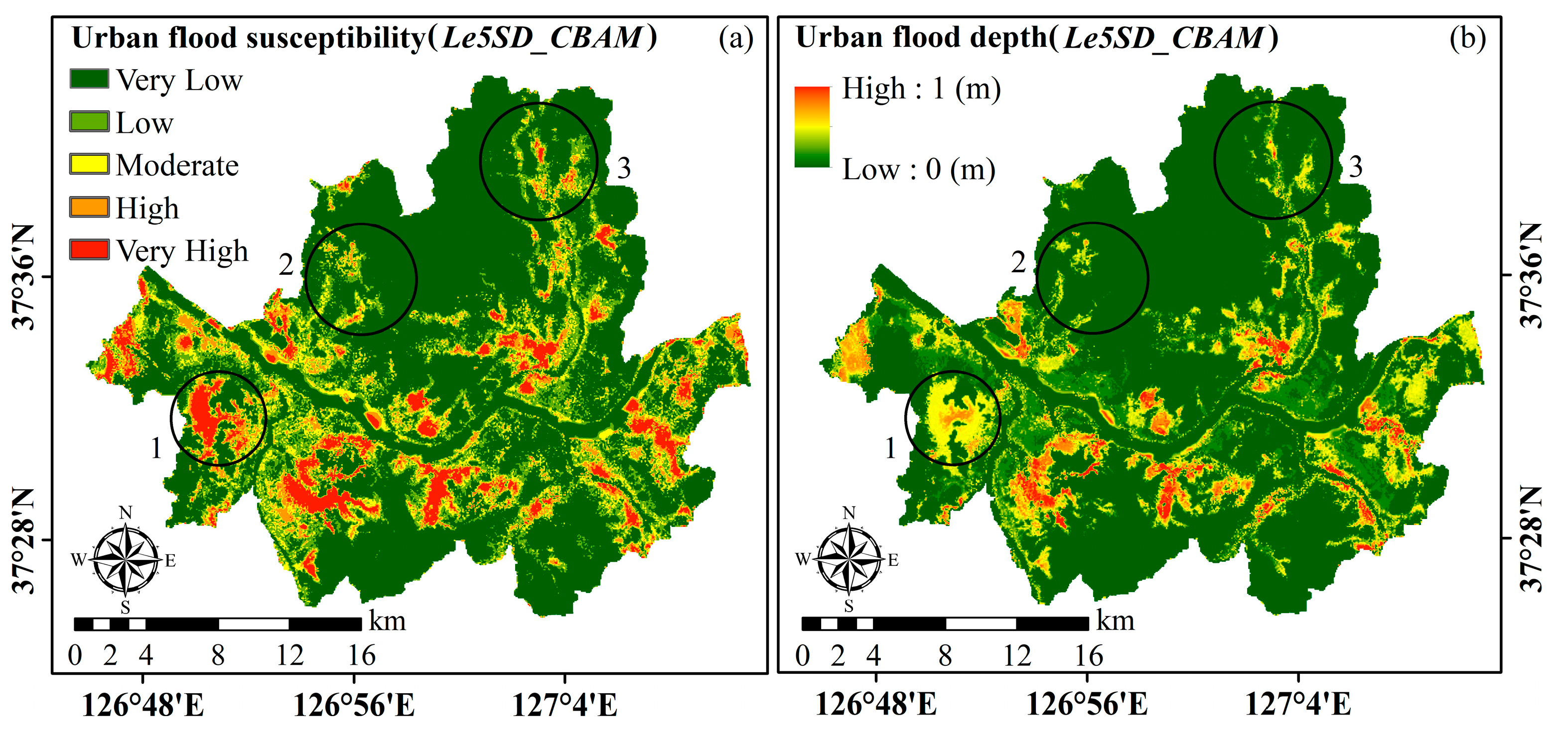
Figure 8a presents the spatial distribution of urban flood susceptibility in Seoul, derived from the Le5SD_CBAM model. The flood susceptibility index ranges from 0 (very low) to 1 (very high) and was reclassified into five distinct levels—Very Low, Low, Moderate, High, and Very High—using the natural breaks (Jenks [73]) optimization method, which is widely applied in hydrological and flood hazard studies [49,58,74]. The resulting susceptibility map indicates that zones categorized as “High” and “Very High” are primarily concentrated along riverbanks and in the central and southeastern regions of the city. These areas typically exhibit low elevation, high surface runoff potential, and elevated TWI values, which collectively contribute to increased flood susceptibility. Areas classified as “Moderate” are widely distributed across the central part of Seoul, forming a transitional buffer between high-susceptibility southern areas and lower-susceptibility northern zones. In contrast, the “Low” and “Very Low” susceptibility classes are mainly located in the northern and western districts, corresponding with elevated terrain and more favorable natural drainage conditions.
The predicted flood depth distribution generated by the Le5SD_CBAM regression model is shown in Figure 8b. Predicted flood depths range from 0 to approximately 1.0 m, with a color gradient used to visualize the severity of inundation. Spatial patterns of flood depth display considerable heterogeneity, with the highest predicted depths found in central and eastern districts—areas characterized by low-lying topography, impervious surfaces, and disrupted drainage pathways. Although much of the urban area exhibits low-to-moderate flood depths, the depth map closely aligns with topographic depressions and areas of impaired hydrologic flow. Notably, certain zones with elevated flood depth do not always correspond to areas of high susceptibility, reflecting the spatial complexity of urban flood behavior.
A spatial comparison between the susceptibility and depth maps highlights both inconsistencies and meaningful correlations across the study area. Three representative zones (circled 1 to 3) illustrate these dynamics: In Zone 1 (southwestern Seoul), flood susceptibility is high to very high, yet flood depths remain moderate, suggesting high vulnerability without substantial water accumulation. In Zone 2 (northcentral Seoul), high susceptibility is paired with shallow predicted depth, likely due to effective drainage infrastructure. Zone 3 (northeastern Seoul) reveals areas with moderate-to-high susceptibility and variable predicted depths ranging from low to high, underscoring the intricate interaction between flood probability and actual inundation severity. These observations emphasize the multifaceted nature of urban flooding and highlight the utility of the bivariate-output CBAM-based model in capturing fine-scale spatial variability in flood risk.

4.3. Variable Importance Assessment

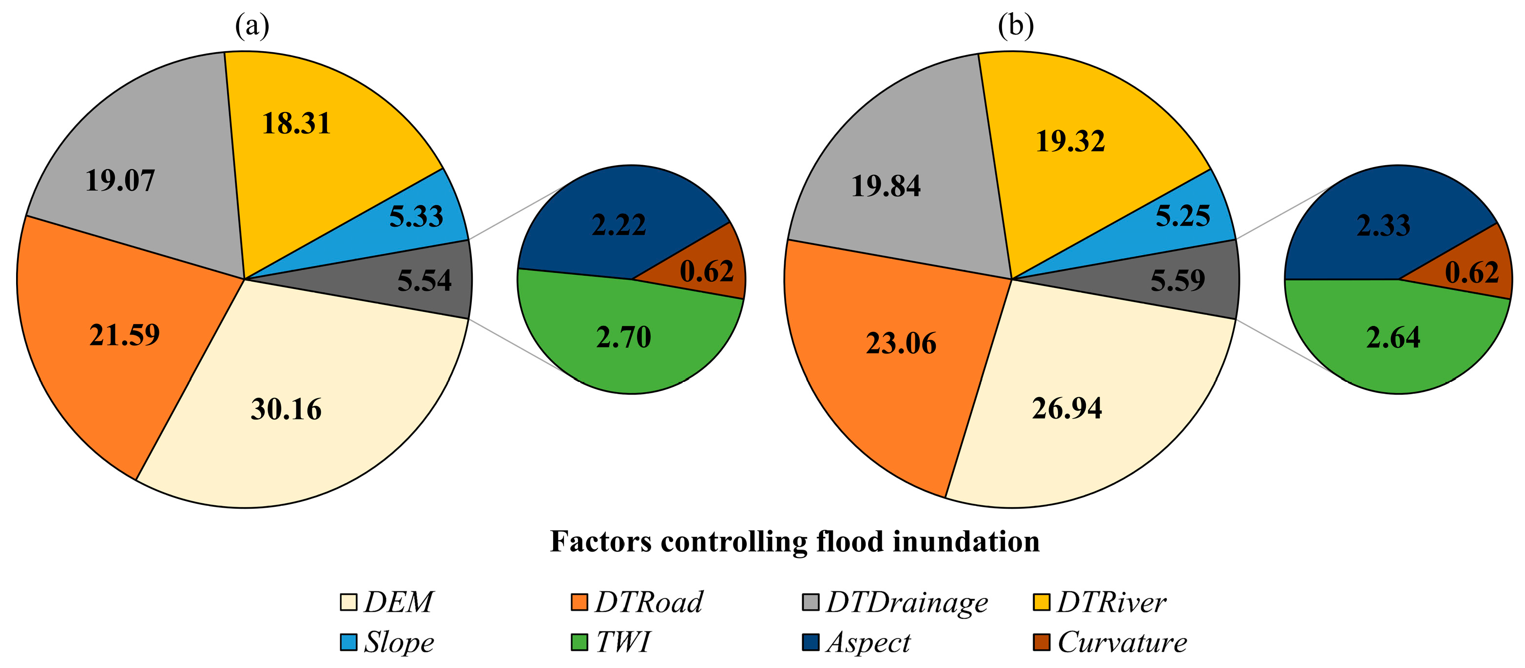
Figure 9a shows the relative contributions of input variables to flood susceptibility prediction. DEM was the most influential factor, accounting for 30.16% of the total contribution, indicating that elevation plays a pivotal role in identifying flood-prone areas. DTRoad was the second most significant factor at 21.59%, reflecting the importance of urban infrastructure in shaping flood susceptibility. DTDrainage and DTRiver contributed 19.07% and 18.31%, respectively, underscoring the critical influence of both engineered and natural hydrological networks. In contrast, slope (5.33%), TWI (2.70%), aspect (2.22%), and curvature (0.62%) had relatively minor contributions. These results suggest that flood susceptibility is primarily governed by terrain characteristics and proximity to water conveyance systems, while secondary topographic indices provide additional spatial nuance.
Figure 9b illustrates the contributions of the same variables to flood depth estimation using the Le5SD_CBAM model. DEM remained the most influential variable, contributing 26.94%, reinforcing its role in predicting potential water accumulation zones. DTRoad (23.06%), DTDrainage (19.84%), and DTRiver (19.32%) followed, showing balanced interplay between anthropogenic and natural drainage pathways. Other factors exhibited minimal changes: slope slightly decreased to 5.25%, TWI stayed stable at 2.64%, aspect increased marginally to 2.33%, and curvature remained the least influential at 0.62%. Together, these findings highlight the consistent importance of elevation and spatial proximity variables in both classification and regression tasks, while contextual terrain features provide complementary insights.

5. Discussion

5.1. Implications of Attention and Bivariate-Output Learning

This study evaluated six CNN-based models for urban flood prediction, focusing on both flood susceptibility classification and flood depth regression. Results demonstrate that integrating CBAM modestly improves model performance. In particular, Le5SD_CBAM, which combines attention mechanisms and bivariate-output learning, consistently outperformed other models across both tasks.
The CBAM-equipped models achieved notably higher accuracy and AUC in classification, indicating improved spatial feature learning and robustness. For instance, Le5SD_CBAM achieved an AUC of 0.91 and accuracy of 83% on the test set, surpassing non-attention models by a clear margin. This suggests that CBAM’s dual focus on channel- and spatial-wise attention helps the network concentrate on flood-relevant features while reducing noise, enhancing generalization.
From a regression standpoint, Le5SD_CBAM also recorded the lowest error values (MAE and RMSE), further supporting the utility of multitask architectures. Importantly, the bivariate-output design appears to function as a form of implicit regularization, improving learning efficiency by capturing shared patterns relevant to both susceptibility and depth estimation. This aligns with the theoretical foundations of multitask learning [75] and demonstrates that joint learning can boost performance without overfitting, even in complex urban flood environments. Compared to previous studies, the proposed model demonstrates competitive performance, achieving an AUC of 0.91 and an RMSE of 0.18 m. These results are in line with or exceed those reported in similar urban flood prediction studies using conventional CNNs (AUC = 0.84, RMSE = 0.163 m), 2D feedforward CNNs (AUC = 0.83), and logistic regression models (AUC = 0.86) [24,29,76]. Overall, the findings underscore the importance of combining attention mechanisms with bivariate-output learning to enhance both predictive accuracy and model robustness, offering promising directions for operational flood risk mapping in data-constrained urban settings.

5.2. Capturing Complementary Aspects of Urban Flood Likelihood and Severity

The Le5SD_CBAM model generates realistic flood predictions across Seoul. These predictions align with established hydrological theory. They also correspond to urban topographic patterns. High and very high susceptibility zones are concentrated along riverbanks and in the central and southeastern districts, where low elevation and poor drainage capacity naturally facilitate surface water accumulation. These patterns correspond closely with historical flood impacts, particularly during the 2010 and 2011 flood events that severely affected the Gangnam area and regions near the Han River [77,78], supporting the model’s predictive validity.
Moderate susceptibility areas form a transitional band across central Seoul, separating high-risk southern zones from lower-risk northern sectors. These zones are characterized by intermediate elevation, heterogeneous land cover, and varied surface permeability, resulting in complex runoff behavior that demands nuanced flood management strategies. Conversely, low and very low susceptibility classifications prevail in the northern and western regions, reflecting higher terrain and naturally favorable drainage conditions. These spatial trends align well with prior studies identifying elevation as a principal determinant of urban flood susceptibility [24,27,77].
Flood depth mapping reveals a more intricate spatial pattern compared to susceptibility classification. Localized zones with predicted depths nearing 1.0 m are found primarily in central and eastern districts, aligning with topographic depressions and areas with impaired flow. These patterns highlight the combined effects of terrain, hydrologic pathways, and anthropogenic modifications on water accumulation and underscore the model’s ability to resolve sub-grid variations in inundation severity [79].
A spatial cross-analysis of susceptibility and depth reveals three representative zones exhibiting divergent outcomes. In Zone 1 (southwestern Seoul), susceptibility is high, but predicted depths are moderate, suggesting the presence of efficient drainage despite vulnerability. Zone 2 (northcentral Seoul) shows high susceptibility and low depth, likely due to robust flood infrastructure mitigating hazard realization. Zone 3 (northeastern Seoul) exhibits a broad range of flood depths within moderately susceptible areas, reflecting localized terrain and infrastructure effects. These spatial contrasts illustrate the value of bivariate-output modeling for capturing the decoupled yet complementary aspects of flood likelihood and severity, providing a nuanced basis for risk-informed urban flood planning.

5.3. Prioritizing Predictors for Future Dual-Output Flood Models

The variable importance analysis reveals key flood prediction factors. Topographic and proximity variables dominate urban flood dynamics. Elevation consistently ranks as the most influential predictor for both tasks. This confirms elevation’s fundamental role in built environments, consistent with previous urban flood studies [80,81]. Meanwhile, proximity to roads, drainage channels, and rivers collectively contributed over half of the predictive power, illustrating how urban infrastructure modifies natural hydrological behavior.
Of particular note is the heightened importance of DTRoad in flood depth prediction. These findings align with observations by Jha et al. (2012) [82], Hammond et al. (2013) [43], Yin et al. (2016) [63], and Palla et al. (2017) [83]. This reflects how impervious surfaces such as road networks govern local water accumulation, especially in topographically constrained or poorly drained zones. The CBAM attention module enhances the model’s focus on such features, as seen in the consistently high attribution scores for DTRoad across both tasks.
Secondary variables like slope, TWI, aspect, and curvature had marginal influence, which aligns with prior studies in urbanized settings, where natural terrain effects are often masked by engineered drainage systems [24,77,81]. The subtle differences in variable rankings between susceptibility and depth tasks validate the utility of bivariate-output learning, allowing the model to capture nuanced, task-specific interactions. This joint-learning framework thus provides a more holistic understanding of flood risk drivers, supporting more informed and location-sensitive flood mitigation planning.

5.4. Implications of Flood Depth Prediction Under Constrained Input Conditions

In data-driven flood modeling, the predictive accuracy of flood depth estimation is highly dependent on the diversity and richness of input variables. In scenarios where key hydrodynamic drivers—such as rainfall intensity, upstream discharge, and drainage system capacity—are unavailable, the model must rely solely on static or semi-static topographic and infrastructural predictors. While such constrained input conditions limit the ability to capture dynamic flood processes in real time, flood depth can still be reasonably inferred in relative terms using spatial patterns of terrain features and proximity to hydrological structures. However, this approach cannot fully represent temporal variability, event-specific rainfall–runoff relationships, or infrastructure performance under different loading conditions. As a result, predicted depths should be interpreted as indicative of spatial flood severity gradients rather than absolute measurements. Despite these limitations, the value of such modeling lies in its ability to support vulnerability mapping, hotspot identification, and risk prioritization in data-sparse environments, offering a practical decision-support tool where traditional hydraulic modeling is infeasible.

5.5. Advantages of Joint Modeling of Flood Susceptibility and Depth

Despite using identical input variables, jointly modeling flood susceptibility and inundation depth within a single AI framework offers distinct advantages over separate single-task models. First, susceptibility and depth are inherently related, as both are influenced by shared hydrological and infrastructural drivers. A bivariate-output model facilitates mutual learning between tasks by capturing complementary patterns, leading to enhanced generalization and predictive performance. Second, simultaneous prediction reduces the risk of logical inconsistencies—such as predicting significant inundation depth in areas classified as non-flood-prone—thereby improving the internal coherence of the results. Third, by sharing a common architecture with hard parameter sharing, the model improves computational efficiency while minimizing redundancy in training. Furthermore, this integrated structure allows for a more comprehensive spatial understanding of urban flood dynamics, providing both binary risk identification and continuous severity estimation. Such dual-task outputs are especially valuable for practical flood risk management, enabling decision-makers to prioritize intervention strategies not only based on flood likelihood but also on expected severity. Overall, the bivariate framework yields richer, more actionable insights than univariate approaches, even when trained on the same set of predictors.

6. Conclusions

This study developed and evaluated six LeNet-5-based deep learning models for the joint prediction of urban flood susceptibility and inundation depth in Seoul, South Korea. Among these, the Le5SD_CBAM model—featuring a bivariate-output architecture integrated with the Convolutional Block Attention Module (CBAM)—exhibited the most robust and reasonably balanced performance across both classification and regression tasks. It achieved a testing accuracy of 83% and an AUC of 0.91 for flood susceptibility classification, along with strong regression performance (MAE: 0.12 m; RMSE: 0.18 m) for flood depth estimation. These results confirm that the incorporation of attention mechanisms and bivariate-output learning structures can significantly improve model generalization and support more comprehensive flood risk assessments.
This study introduces a novel bivariate-output CNN with spatial attention specifically designed for integrated urban flood prediction at the city scale. By simultaneously estimating both flood susceptibility and inundation depth, the proposed framework enhances internal consistency between outputs and offers richer insights for spatial flood analysis. Leveraging a lightweight LeNet-5 backbone and CBAM attention, the model maintains high computational efficiency, making it suitable for practical deployment in large, data-rich urban settings.
The spatial prediction outputs were in close agreement with established hydrological principles, with high flood susceptibility zones predominantly located in low-lying central and southeastern areas. In contrast, the predicted flood depth map revealed more complex spatial variability, highlighting localized areas of inundation where infrastructure limitations or subtle topographic depressions led to unexpected water accumulation. Notably, the model also identified spatial mismatches between flood susceptibility and depth, underscoring the importance of considering both hazard likelihood and severity when assessing urban flood risk.
The variable importance analysis offered valuable insights into the drivers of urban flood vulnerability. Elevation (DEM) emerged as the most influential variable across both prediction tasks, reaffirming the foundational role of topography in flood processes. Proximity-related variables—including distance to roads, drainage, and rivers—jointly contributed a majority of the model’s predictive power, reflecting the strong influence of anthropogenic infrastructure on flood dynamics. Conversely, secondary topographic attributes such as slope, aspect, TWI, and curvature showed relatively limited importance, highlighting the altered hydrological behavior typical of highly urbanized environments, where engineered systems often override natural drainage pathways. Nevertheless, the interactions and combined effects of these variables under different conditions remain insufficiently explored and warrant further investigation.
Despite the strong performance of the proposed model, several limitations can be acknowledged. The current framework does not include real drainage infrastructure or dynamic flood drivers such as rainfall intensity or upstream inflows, which limits its ability to simulate temporal flood behavior. Under such constrained input conditions, flood depth predictions should be interpreted as indicative spatial gradients rather than precise measurements, offering value mainly for hotspot identification and vulnerability mapping in data-scarce settings.
This study also underscores the advantages of bivariate-output learning. By jointly predicting flood susceptibility and depth, the model captures shared hydrological patterns and enhances generalization compared to single-task models. It reduces inconsistencies between outputs and offers a more coherent spatial understanding of flood risk. However, as the current evaluation was limited to a single urban setting (Seoul), the spatial and temporal generalizability of the model remains uncertain. Future research should address the current model’s prediction-focused nature by incorporating dynamic data inputs and enhancing interpretability while also testing its applicability across diverse urban environments to improve both generalizability and understanding of underlying hydrological mechanisms.

Author Contributions

Conceptualization, T.T.L. and J.K.; methodology, T.T.L. and J.K.; formal analysis, T.T.L., T.Q.V. and J.K.; writing—original draft preparation, T.T.L.; writing—review and editing, T.T.L., T.Q.V. and J.K.; visualization, T.T.L.; funding acquisition, J.K. All authors have read and agreed to the published version of the manuscript.

Funding

This work was supported by the 2025 Research Fund of the University of Ulsan.

Data Availability Statement

Data will be made available on request.

Conflicts of Interest

The authors declare no conflicts of interest.

References

  1. Ivanov, V.Y.; Tran, V.N.; Huang, W.; Murphy, K.; Daneshvar, F.; Bednar, J.H.; Alexander, G.A.; Kim, J.; Wright, D.B. Urban flooding is intensified by outdated design guidelines and a lack of a systems approach. Nat. Cities 2024, 1, 626–627. [Google Scholar] [CrossRef]
  2. Dhiman, R.; VishnuRadhan, R.; Eldho, T.I.; Inamdar, A. Flood risk and adaptation in Indian coastal cities: Recent scenarios. Appl. Water Sci. 2018, 9, 5. [Google Scholar] [CrossRef]
  3. Cherqui, F.; Belmeziti, A.; Granger, D.; Sourdril, A.; Le Gauffre, P. Assessing urban potential flooding risk and identifying effective risk-reduction measures. Sci. Total Environ. 2015, 514, 418–425. [Google Scholar] [CrossRef]
  4. Karamouz, M.; Hosseinpour, A.; Nazif, S. Improvement of Urban Drainage System Performance under Climate Change Impact: Case Study. J. Hydrol. Eng. 2011, 16, 395–412. [Google Scholar] [CrossRef]
  5. UN-Water. UN-Water, 2020. Water and Climate Change; United Nations World Water Development Report 2020; UNESCO: Paris, France, 2020. [Google Scholar]
  6. Mosavi, A.; Ozturk, P.; Chau, K.-w. Flood Prediction Using Machine Learning Models: Literature Review. Water 2018, 10, 1536. [Google Scholar] [CrossRef]
  7. Teng, J.; Jakeman, A.J.; Vaze, J.; Croke, B.F.W.; Dutta, D.; Kim, S. Flood inundation modelling: A review of methods, recent advances and uncertainty analysis. Environ. Model. Softw. 2017, 90, 201–216. [Google Scholar] [CrossRef]
  8. Zhou, Q.; Teng, S.; Situ, Z.; Liao, X.; Feng, J.; Chen, G.; Zhang, J.; Lu, Z. A deep-learning-technique-based data-driven model for accurate and rapid flood predictions in temporal and spatial dimensions. Hydrol. Earth Syst. Sci. 2023, 27, 1791–1808. [Google Scholar] [CrossRef]
  9. Karim, F.; Armin, M.A.; Ahmedt-Aristizabal, D.; Tychsen-Smith, L.; Petersson, L. A Review of Hydrodynamic and Machine Learning Approaches for Flood Inundation Modeling. Water 2023, 15, 566. [Google Scholar] [CrossRef]
  10. Kabir, S.; Patidar, S.; Xia, X.; Liang, Q.; Neal, J.; Pender, G. A deep convolutional neural network model for rapid prediction of fluvial flood inundation. J. Hydrol. 2020, 590, 125481. [Google Scholar] [CrossRef]
  11. Kim, J.; Ivanov, V.Y.; Katopodes, N.D. Modeling erosion and sedimentation coupled with hydrological and overland flow processes at the watershed scale. Water Resour. Res. 2013, 49, 5134–5154. [Google Scholar] [CrossRef]
  12. Tran, V.N.; Ivanov, V.Y.; Nguyen, G.T.; Anh, T.N.; Nguyen, P.H.; Kim, D.-H.; Kim, J. A deep learning modeling framework with uncertainty quantification for inflow-outflow predictions for cascade reservoirs. J. Hydrol. 2024, 629, 130608. [Google Scholar] [CrossRef]
  13. Rosenzweig, B.R.; Herreros Cantis, P.; Kim, Y.; Cohn, A.; Grove, K.; Brock, J.; Yesuf, J.; Mistry, P.; Welty, C.; McPhearson, T.; et al. The Value of Urban Flood Modeling. Earth’s Future 2021, 9, e2020EF001739. [Google Scholar] [CrossRef]
  14. Arrighi, C.; Campo, L. Effects of digital terrain model uncertainties on high-resolution urban flood damage assessment. J. Flood Risk Manag. 2019, 12, e12530. [Google Scholar] [CrossRef]
  15. Rahmati, O.; Darabi, H.; Haghighi, A.T.; Stefanidis, S.; Kornejady, A.; Nalivan, O.A.; Tien Bui, D. Urban Flood Hazard Modeling Using Self-Organizing Map Neural Network. Water 2019, 11, 2370. [Google Scholar] [CrossRef]
  16. Apel, H.; Martínez Trepat, O.; Hung, N.N.; Chinh, D.T.; Merz, B.; Dung, N.V. Combined fluvial and pluvial urban flood hazard analysis: Concept development and application to Can Tho city, Mekong Delta, Vietnam. Nat. Hazards Earth Syst. Sci. 2016, 16, 941–961. [Google Scholar] [CrossRef]
  17. Tsakiris, G. Flood risk assessment: Concepts, modelling, applications. Nat. Hazards Earth Syst. Sci. 2014, 14, 1361–1369. [Google Scholar] [CrossRef]
  18. Tran, V.N.; Kim, J. UIDS: A Matlab-based urban flood model considering rainfall-induced and surcharge-induced inundations. Environ. Model. Softw. 2024, 179, 106132. [Google Scholar] [CrossRef]
  19. Sit, M.; Demiray, B.Z.; Xiang, Z.; Ewing, G.J.; Sermet, Y.; Demir, I. A comprehensive review of deep learning applications in hydrology and water resources. Water Sci. Technol. 2020, 82, 2635–2670. [Google Scholar] [CrossRef] [PubMed]
  20. Nguyen, D.H.; Bae, D.-H. Correcting mean areal precipitation forecasts to improve urban flooding predictions by using long short-term memory network. J. Hydrol. 2020, 584, 124710. [Google Scholar] [CrossRef]
  21. Tran, T.D.; Kim, J. Guidance on the construction and selection of relatively simple to complex data-driven models for multi-task streamflow forecasting. Stoch. Environ. Res. Risk Assess. 2024, 38, 3657–3675. [Google Scholar] [CrossRef]
  22. Tran, V.N.; Ivanov, V.Y.; Kim, J. Data reformation–A novel data processing technique enhancing machine learning applicability for predicting streamflow extremes. Adv. Water Resour. 2023, 182, 104569. [Google Scholar] [CrossRef]
  23. Zhao, G.; Pang, B.; Xu, Z.; Cui, L.; Wang, J.; Zuo, D.; Peng, D. Improving urban flood susceptibility mapping using transfer learning. J. Hydrol. 2021, 602, 126777. [Google Scholar] [CrossRef]
  24. Lei, X.; Chen, W.; Panahi, M.; Falah, F.; Rahmati, O.; Uuemaa, E.; Kalantari, Z.; Ferreira, C.S.S.; Rezaie, F.; Tiefenbacher, J.P.; et al. Urban flood modeling using deep-learning approaches in Seoul, South Korea. J. Hydrol. 2021, 601, 126684. [Google Scholar] [CrossRef]
  25. Löwe, R.; Böhm, J.; Jensen, D.G.; Leandro, J.; Rasmussen, S.H. U-FLOOD—Topographic deep learning for predicting urban pluvial flood water depth. J. Hydrol. 2021, 603, 126898. [Google Scholar] [CrossRef]
  26. Jin, H.; Lu, H.; Zhao, Y.; Zhu, Z.; Yan, W.; Yang, Q.; Zhang, S. Integration of an improved transformer with physical models for the spatiotemporal simulation of urban flooding depths. J. Hydrol. Reg. Stud. 2024, 51, 101627. [Google Scholar] [CrossRef]
  27. Seleem, O.; Ayzel, G.; de Souza, A.C.T.; Bronstert, A.; Heistermann, M. Towards urban flood susceptibility mapping using data-driven models in Berlin, Germany. Geomat. Nat. Hazards Risk 2022, 13, 1640–1662. [Google Scholar] [CrossRef]
  28. Li, W.; Wu, J.; Chen, H.; Wang, Y.; Jia, Y.; Gui, G. Unet combined with attention mechanism method for extracting flood submerged range. IEEE J. Sel. Top. Appl. Earth Obs. Remote Sens. 2022, 15, 6588–6597. [Google Scholar] [CrossRef]
  29. Ouma, Y.O.; Omai, L.; Prakash, S. Flood Susceptibility Mapping Using Image-Based 2D-CNN Deep Learning: Overview and Case Study Application Using Multiparametric Spatial Data in Data-Scarce Urban Environments. Int. J. Intell. Syst. 2023, 2023, 5672401. [Google Scholar] [CrossRef]
  30. Yuan, H.; Wang, M.; Li, J.; Zhang, D.; Muhammad Adnan Ikram, R.; Su, J.; Zhou, S.; Wang, Y.; Zhang, Q. Matrix scenario-based urban flooding damage prediction via convolutional neural network. J. Environ. Manag. 2024, 349, 119470. [Google Scholar] [CrossRef]
  31. Shao, Y.; Chen, J.; Zhang, T.; Yu, T.; Chu, S. Advancing rapid urban flood prediction: A spatiotemporal deep learning approach with uneven rainfall and attention mechanism. J. Hydroinform. 2024, 26, 1409–1424. [Google Scholar] [CrossRef]
  32. Yoon, S.-S.; Park, M. Enhancing flood forecasting and warning precision through multi-task deep learning approaches. J. Hydroinform. 2024, 26, 3244–3265. [Google Scholar] [CrossRef]
  33. Pasupa, K.; Sunhem, W. A comparison between shallow and deep architecture classifiers on small dataset. In Proceedings of the 2016 8th International Conference on Information Technology and Electrical Engineering (ICITEE), Yogyakarta, Indonesia, 5–6 October 2016; pp. 1–6. [Google Scholar]
  34. Bejani, M.M.; Ghatee, M. A systematic review on overfitting control in shallow and deep neural networks. Artif. Intell. Rev. 2021, 54, 6391–6438. [Google Scholar] [CrossRef]
  35. Pecheti, S.T.; Ashwaj, U.; Uthej, K.; Murali, K. A Deep Learning Framework for Comparative Analysis in Flood Detection and Area Estimation. Proceedings of 2025 IEEE International Conference on Interdisciplinary Approaches in Technology and Management for Social Innovation (IATMSI), Gwalior, India, 6–8 March 2025; pp. 1–6. [Google Scholar]
  36. Kim, H.-S.; Chung, Y.-S.; Tans, P.P.; Yoon, M.-B. Climatological variability of air temperature and precipitation observed in South Korea for the last 50 years. Air Qual. Atmos. Health 2015, 9, 645–651. [Google Scholar] [CrossRef]
  37. Lee, S.; Choi, Y.; Ji, J.; Lee, E.; Yi, S.; Yi, J. Flood Vulnerability Assessment of an Urban Area: A Case Study in Seoul, South Korea. Water 2023, 15, 1979. [Google Scholar] [CrossRef]
  38. Pour, S.H.; Wahab, A.K.A.; Shahid, S.; Asaduzzaman, M.; Dewan, A. Low impact development techniques to mitigate the impacts of climate-change-induced urban floods: Current trends, issues and challenges. Sustain. Cities Soc. 2020, 62, 102373. [Google Scholar] [CrossRef]
  39. Kim, J.; Sung, H.H.; Choi, G. Spatial Patterns of Urban Flood Vulnerability in Seoul. J. Korean Assoc. Reg. Geogr. 2013, 19, 615–626. [Google Scholar]
  40. Hwang, K.; Schuetze, T.; Amoruso, F. Flood Resilient and Sustainable Urban Regeneration Using the Example of an Industrial Compound Conversion in Seoul, South Korea. Sustainability 2020, 12, 918. [Google Scholar] [CrossRef]
  41. Seo, Y.; Hwang, J.; Noh, S. Analysis of Urban Drainage Networks Using Gibbs’ Model: A Case Study in Seoul, South Korea. Water 2015, 7, 4129–4143. [Google Scholar] [CrossRef]
  42. Maharani, Z.; Kim, J.; Lim, J.H. A Comprehensive Study on Flood Mitigation Strategies of Low-Impact Development in Yeongdeungpo-gu, Seoul. J. Korean Inst. Landsc. Archit. 2024, 52, 83–95. [Google Scholar] [CrossRef]
  43. Hammond, M.J.; Chen, A.S.; Djordjević, S.; Butler, D.; Mark, O. Urban flood impact assessment: A state-of-the-art review. Urban Water J. 2013, 12, 14–29. [Google Scholar] [CrossRef]
  44. Sahoo, S.N.; Sreeja, P. Development of Flood Inundation Maps and Quantification of Flood Risk in an Urban Catchment of Brahmaputra River. ASCE-ASME J. Risk Uncertain. Eng. Syst. Part A Civ. Eng. 2017, 3, A4015001. [Google Scholar] [CrossRef]
  45. Zhao, G.; Xu, Z.; Pang, B.; Tu, T.; Xu, L.; Du, L. An enhanced inundation method for urban flood hazard mapping at the large catchment scale. J. Hydrol. 2019, 571, 873–882. [Google Scholar] [CrossRef]
  46. Tehrany, M.S.; Pradhan, B.; Jebur, M.N. Flood susceptibility mapping using a novel ensemble weights-of-evidence and support vector machine models in GIS. J. Hydrol. 2014, 512, 332–343. [Google Scholar] [CrossRef]
  47. Darabi, H.; Torabi Haghighi, A.; Rahmati, O.; Jalali Shahrood, A.; Rouzbeh, S.; Pradhan, B.; Tien Bui, D. A hybridized model based on neural network and swarm intelligence-grey wolf algorithm for spatial prediction of urban flood-inundation. J. Hydrol. 2021, 603, 126854. [Google Scholar] [CrossRef]
  48. Zhang, W.; Hu, B.; Liu, Y.; Zhang, X.; Li, Z. Urban Flood Risk Assessment through the Integration of Natural and Human Resilience Based on Machine Learning Models. Remote Sens. 2023, 15, 3678. [Google Scholar] [CrossRef]
  49. Zhao, G.; Pang, B.; Xu, Z.; Peng, D.; Zuo, D. Urban flood susceptibility assessment based on convolutional neural networks. J. Hydrol. 2020, 590, 125235. [Google Scholar] [CrossRef]
  50. Khosravi, K.; Shahabi, H.; Pham, B.T.; Adamowski, J.; Shirzadi, A.; Pradhan, B.; Dou, J.; Ly, H.-B.; Gróf, G.; Ho, H.L.; et al. A comparative assessment of flood susceptibility modeling using Multi-Criteria Decision-Making Analysis and Machine Learning Methods. J. Hydrol. 2019, 573, 311–323. [Google Scholar] [CrossRef]
  51. Gumbo., B.; Munyamba., N.; Sithole., G.; Savenije, H.H.G. Coupling of digital elevation model and rainfall-runoff model in storm drainage network design. Phys. Chem. Earth 2022, 27, 755–764. [Google Scholar] [CrossRef]
  52. Seleem, O.; Heistermann, M.; Bronstert, A. Efficient Hazard Assessment for Pluvial Floods in Urban Environments: A Benchmarking Case Study for the City of Berlin, Germany. Water 2021, 13, 2476. [Google Scholar] [CrossRef]
  53. Zhang, S.; Pan, B. An urban storm-inundation simulation method based on GIS. J. Hydrol. 2014, 517, 260–268. [Google Scholar] [CrossRef]
  54. Daly, C.; Neilson, R.; Donald, P. A Statistical-Topographic Model for Mapping Climatological Precipitation over Mountainous Terrain. J. Appl. Meteorol. Climatol. 1994, 33, 140–158. [Google Scholar] [CrossRef]
  55. Rahmati, O.; Pourghasemi, H.R.; Zeinivand, H. Flood susceptibility mapping using frequency ratio and weights-of-evidence models in the Golastan Province, Iran. Geocarto Int. 2015, 31, 42–70. [Google Scholar] [CrossRef]
  56. Choubin, B.; Moradi, E.; Golshan, M.; Adamowski, J.; Sajedi-Hosseini, F.; Mosavi, A. An ensemble prediction of flood susceptibility using multivariate discriminant analysis, classification and regression trees, and support vector machines. Sci. Total Environ. 2019, 651, 2087–2096. [Google Scholar] [CrossRef] [PubMed]
  57. Regmi, A.D.; Devkota, K.C.; Yoshida, K.; Pradhan, B.; Pourghasemi, H.R.; Kumamoto, T.; Akgun, A. Application of frequency ratio, statistical index, and weights-of-evidence models and their comparison in landslide susceptibility mapping in Central Nepal Himalaya. Arab. J. Geosci. 2013, 7, 725–742. [Google Scholar] [CrossRef]
  58. Chapi, K.; Singh, V.P.; Shirzadi, A.; Shahabi, H.; Bui, D.T.; Pham, B.T.; Khosravi, K. A novel hybrid artificial intelligence approach for flood susceptibility assessment. Environ. Model. Softw. 2017, 95, 229–245. [Google Scholar] [CrossRef]
  59. Kirkby, M. Hydrograph modeling strategies. In Process in Physical and Human Geography; Pearson Education Limited: London, UK, 1975; pp. 69–90. [Google Scholar]
  60. Wilson, J.P.; Gallant, J.C. Secondary Topographic Attributes. In Terrain Analysis: Principles and Applications; John Wiley & Sons: New York, NY, USA, 2000; pp. 87–131. [Google Scholar]
  61. O’Neill, E.; Brereton, F.; Shahumyan, H.; Clinch, J.P. The Impact of Perceived Flood Exposure on Flood-Risk Perception: The Role of Distance. Risk Anal. 2016, 36, 2158–2186. [Google Scholar] [CrossRef] [PubMed]
  62. Singh, P.; Sinha, V.S.P.; Vijhani, A.; Pahuja, N. Vulnerability assessment of urban road network from urban flood. Int. J. Disaster Risk Reduct. 2018, 28, 237–250. [Google Scholar] [CrossRef]
  63. Yin, J.; Yu, D.; Yin, Z.; Liu, M.; He, Q. Evaluating the impact and risk of pluvial flash flood on intra-urban road network: A case study in the city center of Shanghai, China. J. Hydrol. 2016, 537, 138–145. [Google Scholar] [CrossRef]
  64. Woo, S.; Park, J.; Lee, J.-Y.; Kweon, I.S. CBAM: Convolutional Block Attention Module. arXiv 2018, arXiv:1807.06521. [Google Scholar] [CrossRef]
  65. Tran, T.D.; Kim, J. Machine learning modeling structures and framework for short-term forecasting and long-term projection of Streamflow. Stoch. Environ. Res. Risk Assess. 2023, 38, 793–813. [Google Scholar] [CrossRef]
  66. Passos, D.; Mishra, P. An automated deep learning pipeline based on advanced optimisations for leveraging spectral classification modelling. Chemom. Intell. Lab. Syst. 2021, 215, 104354. [Google Scholar] [CrossRef]
  67. Sahraei, A.; Houska, T.; Breuer, L. Deep Learning for Isotope Hydrology: The Application of Long Short-Term Memory to Estimate High Temporal Resolution of the Stable Isotope Concentrations in Stream and Groundwater. Front. Water 2021, 3, 740044. [Google Scholar] [CrossRef]
  68. He, M.; Sandhu, P.; Namadi, P.; Reyes, E.; Guivetchi, K.; Chung, F. Protocols for Water and Environmental Modeling Using Machine Learning in California. Hydrology 2025, 12, 59. [Google Scholar] [CrossRef]
  69. Cheng, H.; Zourlidou, S.; Sester, M. Traffic Control Recognition with Speed-Profiles: A Deep Learning Approach. ISPRS Int. J. Geo-Inf. 2020, 9, 652. [Google Scholar] [CrossRef]
  70. Yesilnacar, E.K. The Application of Computational Intelligence to Landslide Susceptibility Mapping in Turkey; University of Melbourne: Parkville, Australia, 2005; p. 200. [Google Scholar]
  71. Williamson, B.D.; Gilbert, P.B.; Carone, M.; Simon, N. Nonparametric variable importance assessment using machine learning techniques. Biometrics 2021, 77, 9–22. [Google Scholar] [CrossRef]
  72. Lundberg, S.M.; Lee, S.I. A unified approach to interpreting model predictions. Advances in neural in-formation processing systems. arXiv 2017, arXiv:1705.07874. [Google Scholar]
  73. Jenks, G.F. The data model concept in statistical mapping. Int. Yearb. Cartogr. 1967, 7, 186–190. [Google Scholar]
  74. Wang, Y.; Fang, Z.; Hong, H.; Peng, L. Flood susceptibility mapping using convolutional neural network frameworks. J. Hydrol. 2020, 582, 124482. [Google Scholar] [CrossRef]
  75. Caruana, R. Multitask Learning. Mach. Learn. 1997, 28, 41–75. [Google Scholar] [CrossRef]
  76. Rahman, M.; Ningsheng, C.; Islam, M.M.; Dewan, A.; Iqbal, J.; Washakh, R.M.A.; Shufeng, T. Flood Susceptibility Assessment in Bangladesh Using Machine Learning and Multi-criteria Decision Analysis. Earth Syst. Environ. 2019, 3, 585–601. [Google Scholar] [CrossRef]
  77. Lee, S.; Kim, J.-C.; Jung, H.-S.; Lee, M.J.; Lee, S. Spatial prediction of flood susceptibility using random-forest and boosted-tree models in Seoul metropolitan city, Korea. Geomat. Nat. Hazards Risk 2017, 8, 1185–1203. [Google Scholar] [CrossRef]
  78. Jo, H. Is it a Disaster or Resources. The Hankyoreh. Available online: https://h21.hani.co.kr/arti/special/special_general/30216.html (accessed on 10 April 2025).
  79. Huang, H.; Chen, X.; Zhu, Z.; Xie, Y.; Liu, L.; Wang, X.; Wang, X.; Liu, K. The changing pattern of urban flooding in Guangzhou, China. Sci. Total Environ. 2018, 622–623, 394–401. [Google Scholar] [CrossRef]
  80. Wang, Y.; Hong, H.; Chen, W.; Li, S.; Panahi, M.; Khosravi, K.; Shirzadi, A.; Shahabi, H.; Panahi, S.; Costache, R. Flood susceptibility mapping in Dingnan County (China) using adaptive neuro-fuzzy inference system with biogeography based optimization and imperialistic competitive algorithm. J. Environ. Manag. 2019, 247, 712–729. [Google Scholar] [CrossRef] [PubMed]
  81. Tehrany, M.S.; Pradhan, B.; Jebur, M.N. Flood susceptibility analysis and its verification using a novel ensemble support vector machine and frequency ratio method. Stoch. Environ. Res. Risk Assess. 2015, 29, 1149–1165. [Google Scholar] [CrossRef]
  82. Jha, A.K.; Bloch, R.; Lamond, J. Cities and flooding: A Guide to Integrated Urban Flood Risk Management for the 21st Century; World Bank Publications: Washington, DC, USA, 2012. [Google Scholar]
  83. Palla, A.; Gnecco, I.; La Barbera, P. The impact of domestic rainwater harvesting systems in storm water runoff mitigation at the urban block scale. J. Environ. Manag. 2017, 191, 297–305. [Google Scholar] [CrossRef] [PubMed]
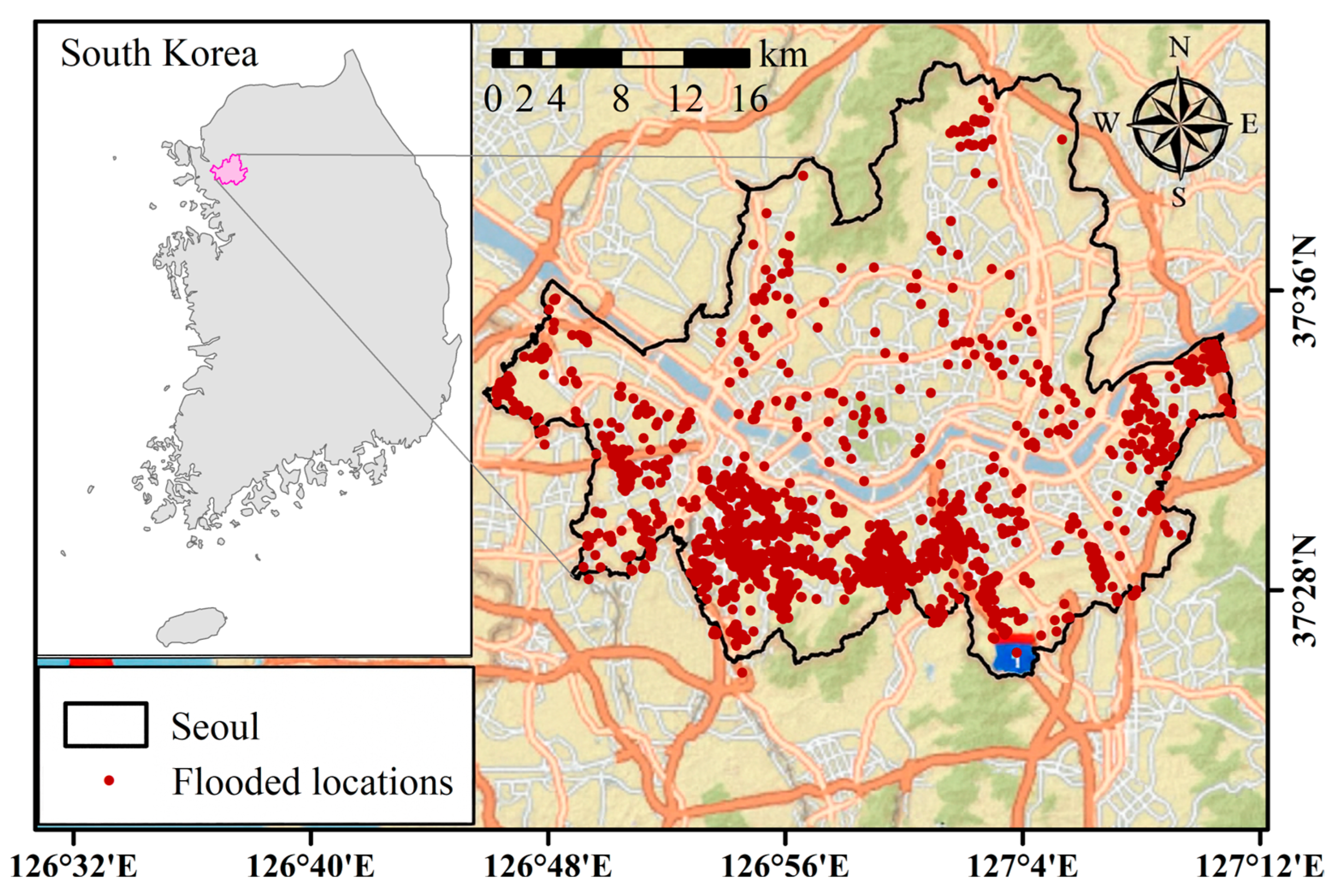
Figure 1. Study area in Seoul (highlighted in pink), South Korea, and distribution of flood-prone locations. A total of 2523 sites, identified from historical flood events between 2010 and 2024, were selected for model development. Flood data were obtained from the Seoul Metropolitan Government database.
Mathematics 13 02617 g001
Figure 2. Spatial distribution of input variables used for flood modeling: (a) DEM, (b) Slope, (c) Aspect, (d) TWI, (e) Curvature, (f) DTRiver, (g) DTRoad, and (h) DTDrainage. All layers were resampled to a 30 × 30 m resolution and normalized to model input. In each map, colors represent the magnitude of the variable, with the corresponding high (red or warm colors) and low (blue or cool colors) values indicated in the legends. All layers were resampled to a 30 × 30 m resolution and normalized for model input.
Mathematics 13 02617 g002
Figure 3. Schematic representation of the proposed three-step framework for urban flood susceptibility classification and inundation depth estimation. The process involves (1) dataset construction using spatial and infrastructural features; (2) model development based on a LeNet-5 convolutional neural network integrated with a Convolutional Block Attention Module (CBAM); and (3) output generation for flood susceptibility classification and flood depth estimation. SHAP analysis is employed to interpret variable importance. Colors in the diagram denote different categories of elements: green boxes indicate model development components, yellow boxes represent datasets, blue boxes correspond to evaluation metrics. Arrows indicate the direction of workflow and the relationships between successive steps.
Mathematics 13 02617 g003
Figure 4. Architectural diagrams of the six LeNet-5-based deep learning models developed in this study, with detailed layer configurations. The models include univariate-output architectures for flood susceptibility classification (Le5S, Le5S_CBAM) and flood depth prediction (Le5D, Le5D_CBAM), as well as bivariate-output models (Le5SD, Le5SD_CBAM) designed for the simultaneous prediction of both susceptibility and depth using shared convolutional layers and task-specific output branches. Colors in the diagrams indicate the processing stage that generated each feature map: after convolutional layers, max-pooling layers, or CBAM layers. Fully connected (FC) layers are illustrated as layers of white circles, where each circle represents a neuron. Dots inside the circles indicate that each layer contains multiple neurons, with only a portion shown for visualization purposes. Arrows indicate the direction of data flow from the input image, through feature extraction and pooling/attention stages, to the final outputs for flood susceptibility (task 1) and flood depth (task 2).
Mathematics 13 02617 g004
Figure 5. Architectural schematic of CBAM_1 illustrating the sequential attention mechanism. The diagram shows the information flow from the input feature map (F) through channel and spatial attention modules, resulting in a refined feature map (F″). CBAM_1 is implemented at the initial stage with 19 × 19 × 6 feature maps, while a similar CBAM_2 structure is applied to deeper layers for feature maps of different dimensions. In the diagram, distinct colors are used to differentiate the functional blocks (e.g., channel attention in green, spatial attention in orange). Small operator circles denote functions: σ is the sigmoid activation that normalizes the attention map to [0, 1], and ⊗ indicates element-wise multiplication between the attention map and the feature map to yield the refined output. Dashed lines outline the boundaries of each attention module, and arrows represent the direction of data flow through the operations.
Mathematics 13 02617 g005
Figure 6. Flood susceptibility classification performance of all models with 95% confidence intervals, evaluated using Accuracy and Area Under the Receiver Operating Characteristic Curve (AUC) on both training and testing datasets. Results were obtained using 1000 bootstrapped resamples to quantify uncertainty.
Mathematics 13 02617 g006
Figure 7. Flood depth prediction performance of all models with 95% confidence intervals, evaluated using MAE and RMSE for training and testing datasets. Results are based on 1000 bootstrapped resamples to assess uncertainty.
Mathematics 13 02617 g007
Figure 8. Predicted flood susceptibility and inundation depth maps for the Seoul metropolitan area, generated using the Le5SD_CBAM model. (a) Flood susceptibility is classified into five ordinal categories, from very low to very high. (b) Inundation depth is predicted on a continuous scale, ranging from 0 to 1.0 m. Three representative zones (indicated by circles labeled 1–3) are highlighted to illustrate varying spatial relationships between flood likelihood and severity.
Mathematics 13 02617 g008
Figure 9. Relative importance of input variables for (a) flood susceptibility classification and (b) flood depth estimation, as determined using SHapley Additive exPlanations (SHAP) applied to the bivariate Le5SD_CBAM model.
Mathematics 13 02617 g009
Table 1. Comparative review of recent studies on CNN-based flood prediction. The studies are organized by model architecture, prediction type (classification or regression), number of tasks (single- or multitask learning), application domain (e.g., urban or riverine), and whether variable importance analysis was conducted.
StudyCNN ArchitectureFlood Prediction TypeTask—Area of ApplicationVariable Importance Analysis
[25]U-NetDepthSingle—Urban
[23]LeNet-5SusceptibilitySingle—Urban
[27]LeNet-5SusceptibilitySingle—UrbanSHAP
[28]U-Net + CBAMSubmerged RangeSingle—Lake
[29]Custom CNNSusceptibilitySingle—UrbanGain Ratio Index
[30]Custom CNNDepthSingle—Urban
[26]Custom CNNDepthSingle—Urban
[31]U-Net + CBAMDepthSingle—UrbanReplacement feature importance
[32]AutoML—
generated CNN
Risk and Water LevelMultitask—River
This StudyLeNet-5 + CBAMSusceptibility and DepthMultitask—UrbanSHAP
Table 2. Summary of input variables and data sources used for model development.
DataData Source
DEMNational Science Foundation—NSF (https://opentopography.org/)
DTRiver, DTRoad, DTDrainageNational Geographic Information Institute
(https://www.ngii.go.kr/world/mapdownload01_en.html) (accessed on 6 November 2024)
Flooding inventorySeoul Metropolitan Government (https://data.seoul.go.kr/dataList/OA-15636/F/1/datasetView.do) (accessed on 18 October 2024)
Table 3. Optimized hyperparameters for the six LeNet-5-based deep learning models. Hyperparameter tuning was performed using Bayesian Optimization implemented via Keras Tuner.
ModelHyperparameters
Learning
Rate
Dropout
(Susceptibility)
Dropout (Depth)Batch SizeNumber of EpochsFC Units
(Susceptibility)
FC Units (Depth)
Le5S0.00040.4168064
Le5S_CBAM0.00040.4646064
Le5D0.00020.2325080
Le5D_CBAM0.00040.3327080
Le5SD0.00030.40.216406480
Le5SD_CBAM0.0010.30.348506480
Table 4. Comparison of computational efficiency across models.
ModelNumber of ParametersTraining Time [s]Testing Time [s]
Le5S7847570.09
Le5S_CBAM82101170.20
Le5D8903370.09
Le5D_CBAM92661000.21
Le5SD13,128640.11
Le5SD_CBAM134911300.21
Disclaimer/Publisher’s Note: The statements, opinions and data contained in all publications are solely those of the individual author(s) and contributor(s) and not of MDPI and/or the editor(s). MDPI and/or the editor(s) disclaim responsibility for any injury to people or property resulting from any ideas, methods, instructions or products referred to in the content.