Abstract
Domain adaptation is a key approach to ensure that artificial intelligence models maintain reliable performance when facing distributional shifts between training (source) and testing (target) domains. However, existing methods often struggle to simultaneously preserve domain-invariant representations and discriminative class structures, particularly in the presence of complex covariate shifts and noisy pseudo-labels in the target domain. In this work, we introduce Conditional Rényi -Entropy Domain Adaptation, named CREDA, a novel deep learning framework for domain adaptation that integrates kernel-based conditional alignment with a differentiable, matrix-based formulation of Rényi’s quadratic entropy. The proposed method comprises three main components: (i) a deep feature extractor that learns domain-invariant representations from labeled source and unlabeled target data; (ii) an entropy-weighted approach that down-weights low-confidence pseudo-labels, enhancing stability in uncertain regions; and (iii) a class-conditional alignment loss, formulated as a Rényi-based entropy kernel estimator, that enforces semantic consistency in the latent space. We validate CREDA on standard benchmark datasets for image classification, including Digits, ImageCLEF-DA, and Office-31, showing competitive performance against both classical and deep learning-based approaches. Furthermore, we employ nonlinear dimensionality reduction and class activation maps visualizations to provide interpretability, revealing meaningful alignment in feature space and offering insights into the relevance of individual samples and attributes. Experimental results confirm that CREDA improves cross-domain generalization while promoting accuracy, robustness, and interpretability.
Keywords:
domain adaptation; image classification; Rényi’s entropy; class-conditional alignment; noisy labels MSC:
68T05
1. Introduction
A primary challenge in the development of artificial intelligence systems is ensuring that models maintain reliable performance under conditions that differ from those observed during training [1]. Such discrepancies may arise due to changes in the operational environment, variations in acquisition devices, or differences in user population characteristics [2]. These shifts, though often subtle, can significantly impact model behavior and compromise generalization capabilities, even when the underlying task remains unchanged [3]. This vulnerability becomes particularly critical in real-world applications, where it is infeasible to anticipate all possible future scenarios, thus limiting the scalability and trustworthiness of deployed solutions [4]. In this context, validation within the source domain alone proves insufficient to guarantee consistent performance in heterogeneous settings, prompting the development of strategies to mitigate such discrepancies. Among these, domain adaptation has emerged as a key approach, enabling the reuse of pretrained models in new environments by aligning distributions across domains, thereby reducing the need for extensive data collection and annotation in the target domain [5]. The latter not only enhances the efficiency of knowledge transfer, but also supports the creation of more robust and sustainable systems in dynamic and uncertain environments.
Despite the progress achieved through domain adaptation, the problem of generalizing to unseen domains remains only partially resolved. Domain shifts can take complex forms that go beyond marginal discrepancies, affecting the internal structure of learned representations and leading to systematic performance degradation in the target domain [6]. Consequently, adapted models frequently exhibit degraded or inconsistent performance when deployed in unfamiliar environments, especially under shifts in input distributions that are structural and semantic in nature [7]. This limitation arises primarily from the inability to preserve domain-invariant features under covariate shifts, where noise in input features, biased samples, or insufficient representations can degrade the alignment across domains and compromise the stability of the learned models [8]. Second, generalization is further hindered when the learned features lack discriminative power, particularly in the presence of concept shift and noisy labels. These factors distort latent representations and decision boundaries, making it difficult to maintain semantic clarity in the target domain [9]. Third, the absence of interpretability mechanisms impedes the reliable evaluation of whether predictions are based on meaningful semantic signals or on spurious correlations inherited from the source domain [10]. Collectively, these challenges hinder the development of domain-adaptive systems that are accurate, robust, and interpretable.
In response to the challenges inherent in domain adaptation, numerous classical approaches have been proposed, most of which rely on linear transformations to align source and target distributions. These strategies aim to mitigate distributional discrepancies through statistical alignment techniques. Methods such as Correlation Alignment (CORAL) and Subspace Alignment (SA) reduce marginal discrepancy by aligning covariance matrices or projecting data onto orthonormal subspaces [11,12]. Despite their effectiveness under controlled conditions, their reliance on original feature spaces or linear projections makes them susceptible to distortions, noise, and domain-specific biases, hindering the extraction of invariant representations [13]. To address these limitations, geometrically inspired extensions such as Geometric Transfer Learning (GTL) have been developed, incorporating structural constraints between domains [14]. Nonetheless, they depend on linear subspace representations, which fail to adequately preserve the support of the target domain in the presence of data heterogeneity or limited representational capacity [15]. In addition, techniques such as Transfer Joint Matching (TJM), Transfer Component Analysis (TCA), and Maximum Independence Domain Adaptation (MIDA) seek to align both marginal and conditional distributions via linear projections [16,17,18]. Yet, they do not guarantee class separability in the latent space, particularly under concept shift or class imbalance, resulting in ambiguous decision boundaries and diminished discriminative performance [19]. A comparable deficiency is noted in Joint Distribution Adaptation (JDA), which, despite modeling joint alignment, assumes uniform relevance across classes and lacks adaptive mechanisms to address intra-class heterogeneity or instance-level significance [20].
Due to the structural constraints of traditional domain adaptation techniques, particularly the decoupling of feature transformation and prediction phases, deep learning methods have emerged as a more cohesive solution for preserving domain-invariant features across the representation space [21]. These approaches leverage the expressive capabilities of deep neural networks to jointly optimize feature extraction and domain alignment, enhancing adaptability under covariate shift [22]. Adversarial training-based models, including Domain-Adversarial Neural Networks (DANNs) and their extensions, have demonstrated considerable effectiveness in aligning marginal distributions within a shared latent space [23,24]. Still, while these methods reduce global disparities, they often struggle to maintain class separability, as they do not explicitly model conditional structures or discriminative boundaries [25]. To overcome these limitations, hybrid models have emerged that integrate deep learning architectures with statistical alignment objectives, enabling end-to-end optimization for improved domain adaptation performance [26]. These approaches aim to preserve both predictive accuracy and domain invariance by combining supervised losses with the minimization of statistical discrepancies across multiple network layers [27,28]. However, hybrid methods also face challenges, such as gradient conflicts between classification and alignment objectives and semantic misalignment caused by noisy pseudo-labels [29]. In parallel, self-supervised learning (SSL) has been introduced into domain adaptation pipelines to alleviate the dependence on labeled target data, typically by leveraging contrastive objectives to learn transferable features without explicit supervision [30,31,32]. More recently, foundation models—large-scale pretrained architectures with broad generalization capacity—have opened new avenues for adaptation by employing mechanisms such as prompt tuning, adapter modules, or domain-specific fine-tuning [33,34]. While these strategies show promise, their deployment in the presence of domain shift remains constrained by semantic misalignment and high computational cost [35]. Although deep learning has significantly advanced the extraction of domain-invariant features, ensuring discriminative consistency and semantic alignment in the target domain remains a critical challenge [36].
Despite notable advances in deep learning techniques designed to extract domain-invariant features, many of these methods struggle to maintain a discriminative class structure within the target domain [21,22]. To address this, transfer-based strategies—such as fine-tuning, teacher–student models, meta-learning frameworks, and asymmetric architectures like Adversarial Discriminative Domain Adaptation (ADDA)—have been introduced to enhance inter-class separation through adaptive training or auxiliary supervision [25,37,38,39]. However, these methods often suffer from limitations including degradation of pretrained representations and sensitivity to noise [40,41] and the absence of explicit modeling of class boundaries, particularly in ADDA variants [42]. Conditional alignment techniques, such as Conditional Adversarial Domain Adaptation (CDAN), address part of this shortcoming by incorporating classifier outputs into the discriminator, thereby capturing class-conditional dependencies [43]. Nonetheless, they remain vulnerable to class imbalance and low-confidence predictions, which can lead to distorted decision boundaries [36]. In response to these challenges, information-theoretic approaches have emerged as a complementary paradigm, optimizing transfer through objectives based on mutual information or entropy [44,45]. By leveraging strategies such as entropy minimization and the information bottleneck principle, these methods regularize latent representations, thereby mitigating overfitting on the source domain and improving generalization under target shift [46,47,48].
In addition to generalization and discriminability, interpretability has become a pivotal aspect of domain adaptation, especially in high-stakes applications where understanding model behavior is essential for fostering trust, transparency, and accountability [49]. In this context, latent space analysis has proven valuable for examining the structure of learned representations. Linear techniques such as Principal Component Analysis (PCA) offer computational efficiency but fall short in capturing the nonlinear relationships relevant across multiple domains [50]. In contrast, nonlinear methods like t-distributed Stochastic Neighbor Embedding (t-SNE) and Uniform Manifold Approximation and Projection (UMAP) are more effective in representing complex inter-domain structures [51]. UMAP, in particular, stands out for its ability to preserve both local and global structures, maintain stability under parameter variation, and scale efficiently—making it especially useful for visualizing semantic alignment across domains [52,53]. Moreover, interpretability is especially crucial in sensitive applications. Among post hoc methods, Gradient-weighted Class Activation Mapping (Grad-CAM) generates attention maps that highlight regions influencing model predictions, while its extension, Grad-CAM++, improves spatial resolution through higher-order derivatives, though it remains limited by nonlinear activation functions [54,55,56]. In domain adaptation, Grad-CAM++ has proven effective not only as an explainability tool but also for visually assessing semantic consistency across domains [57]. Other approaches, such as Layer-wise Relevance Propagation (LRP) and SHapley Additive exPlanations (SHAP), provide quantitative insights by assigning relevance scores to input features, aiding the identification of spurious patterns or conflicting decision rules [58]. The lack of interpretability methods specifically designed for transfer learning and domain adaptation remains a significant limitation, highlighting the need for more robust explanatory tools tailored to cross-domain scenarios [59].
Here, we propose Conditional Rényi -Entropy Domain Adaptation (CREDA), a novel domain adaptation framework designed to simultaneously preserve domain-invariant representations, enforce class-conditional alignment, and mitigate the effect of noisy pseudo-labels. The core idea of CREDA is to regularize deep feature alignment using a differentiable, matrix-based formulation of Rényi’s quadratic entropy, which provides a non-parametric and robust estimate of class-wise distributional similarity. CREDA is implemented as an end-to-end trainable architecture comprising three key stages:
- –
- Deep Feature Extraction: A shared ResNet-18 backbone encodes samples from both source and target domains into a latent representation space.
- –
- Noise-Aware Label Weighting: An entropy-derived confidence score is used to down-weight low-confidence pseudo-labels in the target domain, improving robustness against noisy or ambiguous predictions.
- –
- Class-Conditional Alignment via Rényi-based entropy: A novel entropy-based regularization term is applied over kernel Gram matrices to minimize divergence between class-wise source and target feature distributions.
We evaluate CREDA on three widely used visual domain adaptation benchmarks for image classification: Digits, ImageCLEF-DA, and Office-31. Additionally, we compare its performance against state-of-the-art methods—including DANN, ADDA, and CDAN+E— across various backbone architectures such as ResNet-18, ResNet-50, and Vision Transformers (ViT). The results consistently demonstrate that CREDA achieves superior performance in terms of classification accuracy, semantic alignment, and interpretability, with improvements of average accuracy across benchmarks. Qualitative analyses using UMAP and Grad-CAM++ further confirm that CREDA maintains both inter-class separability and cross-domain semantic coherence, highlighting its potential for deployment in real-world, label-scarce environments.
2. Materials and Methods
2.1. Kernel Methods Fundamentals
Kernel methods provide a powerful framework for developing nonlinear algorithms. The core idea is to implicitly map the input data from its original space into a high-dimensional, or even infinite-dimensional, feature space via a nonlinear mapping . The space is a special type of Hilbert space known as a Reproducing Kernel Hilbert Space (RKHS), and the mapping is chosen such that complex patterns in the data may become simpler, e.g., linearly separable [60].
Explicitly computing the coordinates of the mapped data points is often computationally expensive or infeasible. Then, the kernel trick allows us to bypass this by defining a kernel function that computes the inner product between two points in the feature space:
Then, we work directly with the kernel function without ever needing to know the explicit form of or the structure of . Indeed, an RKHS is uniquely defined by this property, ensuring that all computations can be performed using the kernel [61]. In practice, a common choice for the kernel function is the Gaussian kernel:
which corresponds to an infinite-dimensional feature space, with . Still, its mathematical tractability and intuitive notion of similarity make it a commonly used approach [62].
2.2. Kernel-Based -Rényi’s Entropy Estimation
Let X be a continuous random variable with a probability density function (PDF) , , the Rényi’s -order entropy is defined as follows [63]:
where , and . A primary challenge in applying this definition is that in most practical scenarios, especially with high-dimensional data like deep features, the underlying PDF is unknown [64]. To circumvent this, a Parzen-window method, also known as Kernel Density Estimation (KDE) can be employed. Namely, given a finite set of N samples , the PDF at any point x can be estimated as the average of kernel functions centered at each sample [65]:
where the Gaussian kernel is selected for its mathematical simplicity and desirable smoothing behavior (see Equation (2)). In particular, when in Equation (3), we focus on the special case of Rényi’s entropy, known as quadratic entropy. Indeed, the integral term in Equation (3), , is known as the Information Potential (IP) [66], a measure of the average information contained in the distribution. Substituting the KDE estimator into the IP integral, yields the following:
A significant advantage of using a Gaussian kernel is that the integral in Equation (5) has a closed-form solution based on the convolution property of Gaussians [67]:
The latter simplifies the IP estimator to a practical, sample-based formula that depends only on pairwise interactions between samples, completely bypassing the need for explicit PDF estimation:
Next, let be a Gram matrix whose elements are the pairwise kernel evaluations, . The sum of all elements in this matrix can be computed as , where is a column vector of ones. This gives a matrix-based estimator for the IP:
Recently, a -Rényi matrix-based operator extracts from the IP expression in Equation (8). More generally, Rényi’s entropy can be defined directly over the eigenspectrum of a normalized Gram matrix. If we define a normalized Gram matrix , where is the trace operator, the entropy is given by [68]:
where are the eigenvalues of . For our work with , we use a computationally stable form based on the Frobenius norm: , where , and This matrix-based formulation is essential for deep learning due to several key properties:
- –
- Non-parametric: It makes no prior assumptions about the underlying data distribution, making it highly suitable for the complex and high-dimensional feature spaces learned by neural networks.
- –
- Differentiable: The entropy loss is a function of the Gram matrix elements, which are themselves differentiable functions of the feature vectors produced by a given network. This allows gradients to be backpropagated through the kernel computations to the network’s parameters, enabling end-to-end training.
- –
- Robust: The entropy is calculated based on the collective geometric structure of the data, as captured by all pairwise interactions in the Gram matrix. This makes the measure inherently robust to outliers, which would have a limited impact on the overall sum of kernel values.
The matrix-based entropy framework in Equation (9) can be extended to measure relationships between two random variables, X and Y, represented by paired feature vectors . This is achieved by defining a joint Gram matrix using the Hadamard (element-wise) product as follows:
- –
- Joint Entropy—(JE). Let and be the Gram matrices computed from the feature sets of X and Y, respectively. The joint entropy based on the -Rényi estimator is defined as follows [69]:where , and ⊙ denotes the Hadamard product. Of note, the joint matrix captures the similarity between pairs of samples in the joint feature space.
- –
- Mutual Information—(MI). It quantifies the statistical dependence between two variables. In the matrix-based framework, it is defined in analogy to its classic information-theoretic definition:where each entropy term is computed from its respective (normalized) Gram matrix. Maximizing MI is a common objective in representation learning, as it encourages a representation to retain information about a relevant variable.
- –
- Conditional Entropy—(CE). It measures the remaining uncertainty in a variable X given that Y is known. It is defined as follows:Minimizing conditional entropy is equivalent to making X more predictable from Y.
2.3. Domain Adaptation with -Rényi Entropy-Based Label Weighting and Regularization
Our proposed method, Conditional -Rényi’s Entropy Regularization (CREDA), is designed for end-to-end training in unsupervised domain adaptation. The framework leverages a deep feature extractor that maps an input image , with to a d-dimensional feature vector , as follows:
where stands for the l-th feature extractor layer (), and ∘ is the function composition operator. Moreover, a classifier that predicts class-probability vector is defined as follows:
with as a given classifier layer (), , and
In practice, we are given a labeled source domain with , , , and . Also, an unlabeled target domain is provided as . For each class c, we compute the source, target, and source-target kernel-based matrices , and as follows:
where , and . Moreover, is the number of samples in , where . Likewise, holds the number of target inputs satisfying .
Here, to enhance robustness against noisy pseudo-labels in the target set, we introduce a confidence weighting scheme derived from a principled, entropy-based measure of prediction uncertainty. The core idea is to quantify the uncertainty of a classifier’s output probability vector, , using its Rényi’s quadratic entropy in Equation (3), as follows:
In turn, to create a universally comparable score, this entropy value is normalized by its theoretical maximum, which occurs for a uniform distribution and is equal to . This yields a normalized uncertainty score , which is bounded in . Therefore, we propose incorporating a confidence weighting vector , derived from the normalized uncertainty score :
where . The latter provides a theoretically grounded mechanism to down-weight ambiguous predictions, a strategy that has proven effective in related contexts for handling label uncertainty [70].
Afterward, a target weighting matrix can be computed, yielding the following:
where .
Now, our CREDA method lies in a novel regularization term that enforces alignment between the class-conditional distributions of the source and target domains. So, we employ a kernel-based quadratic Rényi entropy mutual information estimator (see Section 2.2) and the confidence weighting scheme in Equation (19), as follows:
where , and
which enables the computation of our MI estimator in Equation (21) even when the source and target sample sizes differ, namely .
Finally, the complete CREDA loss integrates the standard supervised cross-entropy on labeled source data with our proposed mutual information regularizer, based on the quadratic Rényi entropy formulation, as follows:
where is a hyperparameter controlling the strength of the domain alignment.
In practice, the computation of the kernel matrices in Equations (15)–(17) in our CREDA loss is performed within each training mini-batch. For a given mini-batch of source and target samples, features are first extracted, and pseudo-labels for the target samples are generated. Subsequently, for each class c, the corresponding feature vectors from the source batch (with ground-truth label c) and the target batch (with pseudo-label c) are filtered. The cross-domain kernel matrix is then computed by evaluating the Gaussian kernel between every filtered source feature and every filtered target feature from the batch. The intra-domain matrices, and , are computed similarly among the respective filtered features. If a class is not present in a given mini-batch, its contribution to the regularization loss for that training step is zero. This batch-wise, class-conditional procedure allows for an efficient and scalable implementation of our proposed alignment objective.
Remarkably, the selection of Rényi’s quadratic entropy () is motivated by its direct connection to the IP in Equation (5), which, under a Gaussian kernel, translates the alignment objective into a geometrically intuitive goal [63]. Specifically, the sample-based estimator in Equation (7) becomes a sum of pairwise similarities, meaning that minimizing our class-conditional loss in Equation (23) is equivalent to encouraging feature vectors of the same class to form tight, pure clusters in the feature space, directly promoting class separability. Furthermore, our approach is sensitive to higher-order statistics; thereby, CREDA-based loss captures the overall structure of the distributions, such as their dispersion and modality, which is critical for aligning complex, multi-modal classes often found in real-world datasets. Finally, the estimator’s formulation as an average over all pairwise interactions provides a robust estimate of class-wise distributional similarity. This inherent averaging makes the gradient estimates stable by mitigating the influence of individual outliers or noisy pseudo-labels, a common challenge in unsupervised settings.
Moreover, in discussing the convergence properties of our CREDA loss, it is crucial to distinguish between the statistical consistency of the estimator and the empirical convergence of the deep learning model during training. The mutual information estimator in Equation (21) inherits strong theoretical properties from its foundation in Parzen-window kernel estimation (see Equation (4)). As established in non-parametric statistics, KDE provides a consistent estimator, meaning the estimated probability density converges to the true underlying density as the number of samples approaches infinity [65]. Consequently, the IP at the core of our approach, and by extension our full mutual information estimator, are also statistically consistent estimators of the true quadratic Rényi’s mutual information between the class-conditional distributions. Now, from an optimization perspective, the complete CREDA loss is non-convex due to the highly nonlinear nature of deep approaches. Therefore, formal guarantees of convergence to a global minimum are not feasible, a common characteristic of deep learning systems. Still, our method is designed to facilitate stable empirical convergence. The use of an infinitely differentiable Gaussian kernel ensures our regularization term is smooth, contributing to a well-behaved loss landscape that is conducive to gradient-based optimization.
Figure 1 summarizes the core components and training pipeline of our proposed CRERDA model for conditional domain adaptation.

Figure 1.
CREDA framework for domain adaptation, incorporating classification loss and -Rényi Entropy-based label weighting and regularization to attain domain alignment with a class-aware structure. Blue: source, Red: target, Purple: shared.
3. Experimental Set-Up
To rigorously evaluate the effectiveness of the proposed CREDA framework for domain adaptation in image classification tasks, we present a comprehensive analysis that includes descriptions of the benchmark datasets, training protocols, comparative baselines, and quantitative and qualitative performance assessments.
3.1. Tested Datasets
To assess the effectiveness and robustness of the proposed domain adaptation method, we conducted extensive experiments on three widely recognized benchmark datasets commonly used in domain adaptation research. Each dataset encompasses visual domains exhibiting substantial distribution shifts, thereby providing a challenging setting for learning domain-invariant representations, as detailed below:
- –
- Digits: This benchmark suite is designed for evaluating domain adaptation on digit recognition tasks, spanning both handwritten and natural-scene digits. It comprises three standard datasets: MNIST (M), a large database of handwritten digits; USPS (U), another handwritten digit set characterized by its lower resolution; and SVHN (S), which contains house numbers cropped from real-world street-level images [71]. Notably, the S domain is particularly challenging due to its significant variability in lighting, background clutter, and visual styles compared to M and U (see Figure 2).
 Figure 2. Representative input images for each digit class across source and target domains.
 - –
- ImageCLEF-DA: This is a standard benchmark for unsupervised domain adaptation, organized as part of the ImageCLEF evaluation campaign. It comprises 12 common object classes shared across three distinct visual domains: Caltech-256 (C), ImageNet ILSVRC 2012 (I), and Pascal VOC 2012 (P), see Figure 3. Each domain contains 600 images, with a balanced distribution of 50 images per class [72]. All images are resized to pixels.
 Figure 3. Representative input images for each object class across source and target domains in the ImageCLEF-DA dataset.
 - –
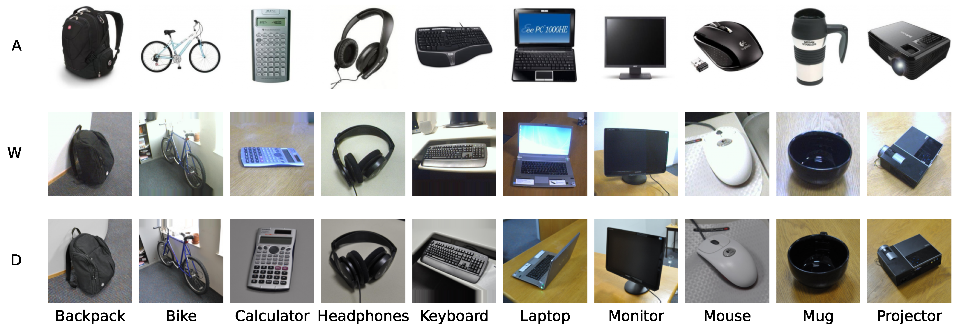
- Office-31: It consists of 4110 images across 31 object classes, sourced from three domains with distinct visual characteristics: Amazon (A), which features centered objects on a clean, white background under controlled lighting; Webcam (W), containing low-resolution images with typical noise and color artifacts; and DSLR (D), which includes high-resolution images with varying focus and lighting conditions [73]. Here, we selected a subset of ten shared classes (see Figure 4).
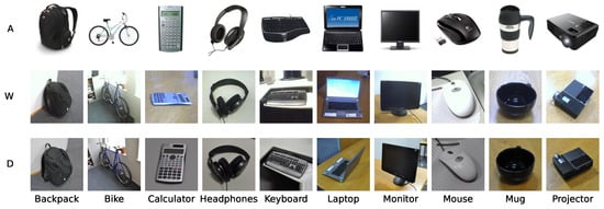 Figure 4. Representative input images for each object class across source and target domains in the Office-31 dataset.
Together, these benchmarks allows evaluating the capacity of domain adaptation methods to generalize across diverse and challenging visual domains.
3.2. Assessment and Method Comparison
To comprehensively evaluate the impact of the feature extractor’s architecture on model performance, we experimented with three distinct backbones: a standard ResNet-18, its deeper counterpart ResNet-50, and a ViT. Each backbone is adapted for feature extraction in domain transfer tasks by removing its final classification layer. The primary baseline is a ResNet-18 convolutional backbone pretrained on ImageNet [74]. To tailor the architecture for our tasks, the final fully connected layer is removed, while all preceding convolutional and residual blocks are retained. This modification enables the extraction of high-level spatial representations that are robust and transferable across domains [75]. A comprehensive description of the ResNet-18 feature extractor’s architecture is provided in Table 1.

Table 1.
Architectural details of the ResNet-18 feature extractor.
Afterward, to investigate the effect of network depth, we also employed a ResNet-50 backbone, a deeper and more powerful variant within the ResNet family [74]. ResNet-50 utilizes bottleneck residual blocks, which are more computationally efficient for deeper networks [76]. Similar to the ResNet-18 configuration, the model is pretrained on ImageNet, and its final fully connected layer is removed to serve as a feature extractor. This results in a 2048-dimensional feature vector. The detailed architecture is presented in Table 2.

Table 2.
Architectural details of the ResNet-50 feature extractor.
Also, to explore an alternative architectural paradigm beyond convolutional networks, we incorporated a ViT-based model, specifically the vit_tiny_patch16_224 variant (termed ViT-Tiny) [77]. Unlike CNNs, ViT-Tiny processes images by splitting them into a sequence of fixed-size patches, which are then linearly embedded and fed into a standard Transformer encoder. For this study, we use a ViT-Tiny pretrained on ImageNet with an input resolution of . The classification head is discarded, and the output embedding of the special [CLS] token from the final Transformer block is used as the feature representation, yielding a 192-dimensional vector. The architecture is detailed in Table 3.

Table 3.
Architectural details of the ViT-Tiny feature extractor.
Moreover, the following domain adaptation strategies are considered for comparison:
- –
- Baseline: A thenceforward approach is trained exclusively on the source domain without any adaptation mechanism, see Figure 5. The optimization objective is to minimize the conventional supervised cross-entropy loss, which serves as a lower bound for performance evaluation under domain shift:
 Figure 5. Baseline model for supervised training on the source domain without adaptation.
 - –
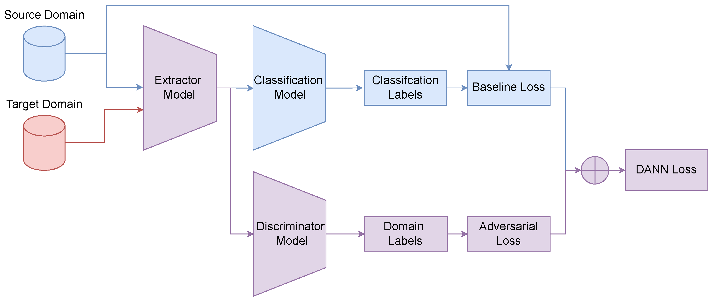
- DANN: The Domain-Adversarial Neural Network (DANN) [78] introduces a domain discriminator, , which is trained to distinguish source features from target ones, see Figure 6. The discriminator is implemented as a multi-layer neural network, where a predicted label of 1 indicates source domain membership, and 0 indicates target domain membership. Moreover, the feature extractor is simultaneously trained to produce features that fool the discriminator, thereby learning domain-invariant representations via a Gradient Reversal Layer (GRL). The overall objective is a minimax game:where represents a trade-off hyperparameter. The domain adversarial loss is the binary cross-entropy for domain classification, where source samples are assigned domain label 0, and target samples label 1.
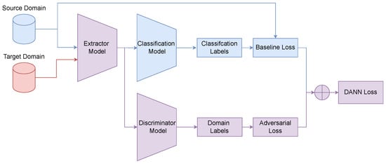 Figure 6. DANN framework for unsupervised domain adaptation. Blue: source, Red: target, Purple: shared.
 - –
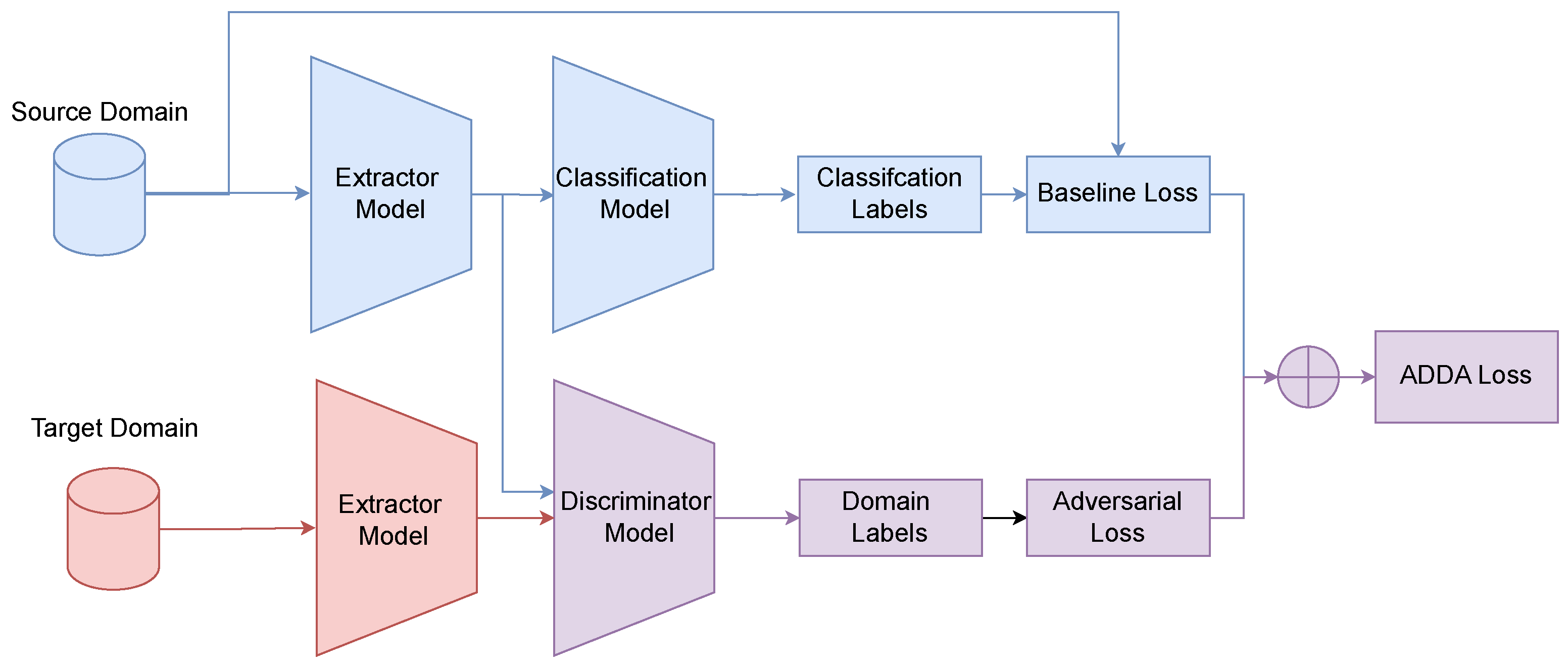
- ADDA: The Adversarial Discriminative Domain Adaptation (ADDA) framework [79] separates the training into two distinct stages, see Figure 7. First, a source feature extractor and the classifier are trained using the supervised loss (see Equation (24)). In the second stage, the parameters of and are frozen. Then, a new target feature extractor, (initialized with the weights in ), is then trained to fool the domain discriminator in a minimax game (see Equation (25)). The objective is to align the target feature distribution with the fixed source feature distribution.
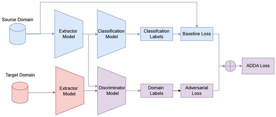 Figure 7. ADDA framework for unsupervised domain adaptation. Blue: source; Red: target; Purple: shared.
 - –
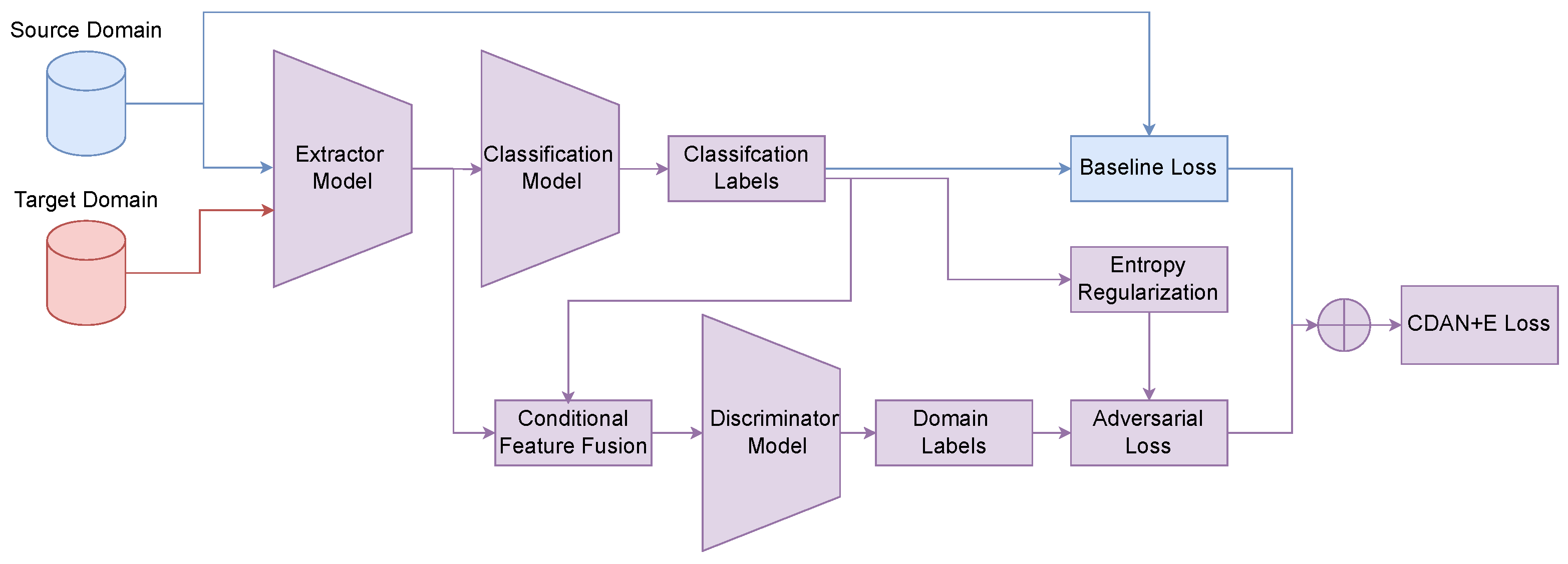
- CDAN+E: The Conditional Domain Adversarial Network (CDAN) [80] enhances adversarial alignment by using a multilinear feature representation, , as input to the domain discriminator . The CDAN+E variant, as implemented in standard benchmarks, employs a sophisticated entropy-based mechanism that serves a dual purpose: it implements entropy minimization for the target domain while simultaneously weighting the adversarial loss to focus on more reliable samples, as seen in Figure 8.
 Figure 8. CDAN+E framework for unsupervised domain adaptation. Blue: source; Red: target; Purple: shared.Specifically, the Shannon entropy is computed for the predictions of all samples in a batch. This entropy value is then used in two ways. First, it is passed through a GRL, which implicitly creates an entropy minimization objective for the feature extractor, encouraging it to produce more confident (low-entropy) predictions. Second, the entropy is transformed into a sample-wise weight, as follows:This weighting scheme gives greater importance to samples with confident predictions (low entropy), thereby focusing the adversarial alignment on well-structured regions of the feature space. The resulting weighted conditional adversarial loss, , is then defined as follows:where both and are calculated according to Equation (26). The total loss for the CDAN+E framework can thus be expressed as the combination of the supervised loss and this integrated adversarial and entropy-regularized objective (see Equation (25)).
Overall, two main components are employed depending on the training objective: a label classifier for supervised task learning and a domain discriminator for adversarial domain adaptation. Namely, the label classifier transforms the feature vector of dimension d, produced by the backbone, into a vector of C class logits. The value of d depends on the specific feature extractor employed (e.g., 512 for ResNet-18, 2048 for ResNet-50, and 192 for ViT-Tiny). The corresponding architecture is presented in Table 4.

Table 4.
Architecture of the generic label classifier.
In adversarial training, a domain discriminator is employed to differentiate between source and target samples, thereby promoting domain-invariant feature extraction. Its input dimension d is determined by the underlying method. For instance, DANN and ADDA use the feature vector directly, while CDAN+E utilizes the outer product between features and class predictions, yielding an input dimension . The architecture, which mirrors the general structure of the label classifier, is detailed in Table 5.

Table 5.
Architecture of the generic domain discriminator.
In all experimental scenarios, we report the classification accuracy and its associated standard deviation in the test set of the target domain. Moreover, during training, model performance is periodically evaluated on validation subsets drawn from both source and target domains to monitor intermediate generalization behavior. In this sense, the Accuracy (ACC) measure is defined as follows:
where and denote the predicted and ground truth labels, respectively. is the indicator function that returns 1 if the condition is true and 0 otherwise. The standard deviation is estimated from the batch-wise accuracies, serving as a proxy for model stability during inference. The Baseline model is trained solely on labeled samples from the source domain and is directly evaluated in the target domain without any adaptation mechanisms. This setting establishes a lower bound for performance under domain shift conditions.
In addition to quantitative measures, we assess the discriminative quality of the learned feature representations using qualitative techniques. Specifically, we employ the well-known Uniform Manifold Approximation and Projection (UMAP) [52], a nonlinear dimensionality reduction technique to project high-dimensional features into a two-dimensional latent space, enabling visual inspection of inter-domain and inter-class separability [81]. This technique facilitates an empirical evaluation of how well the feature extractor captures semantically consistent structures across domains. To further complement this analysis, we apply the GradCAM++ method to the classifier module in order to visualize spatial attention regions associated with individual predictions [82]. These attention maps provide insight into the decision-making process of the model and support a comparative interpretation of class activation patterns across source and target domains.
3.3. Training Details
The training procedure follows the standard protocol for unsupervised domain adaptation: all labeled data from the source domain are used along with the entire set of unlabeled data from the target domain. The latter approach aims to learn domain-invariant representations without requiring explicit supervision in the target domain.
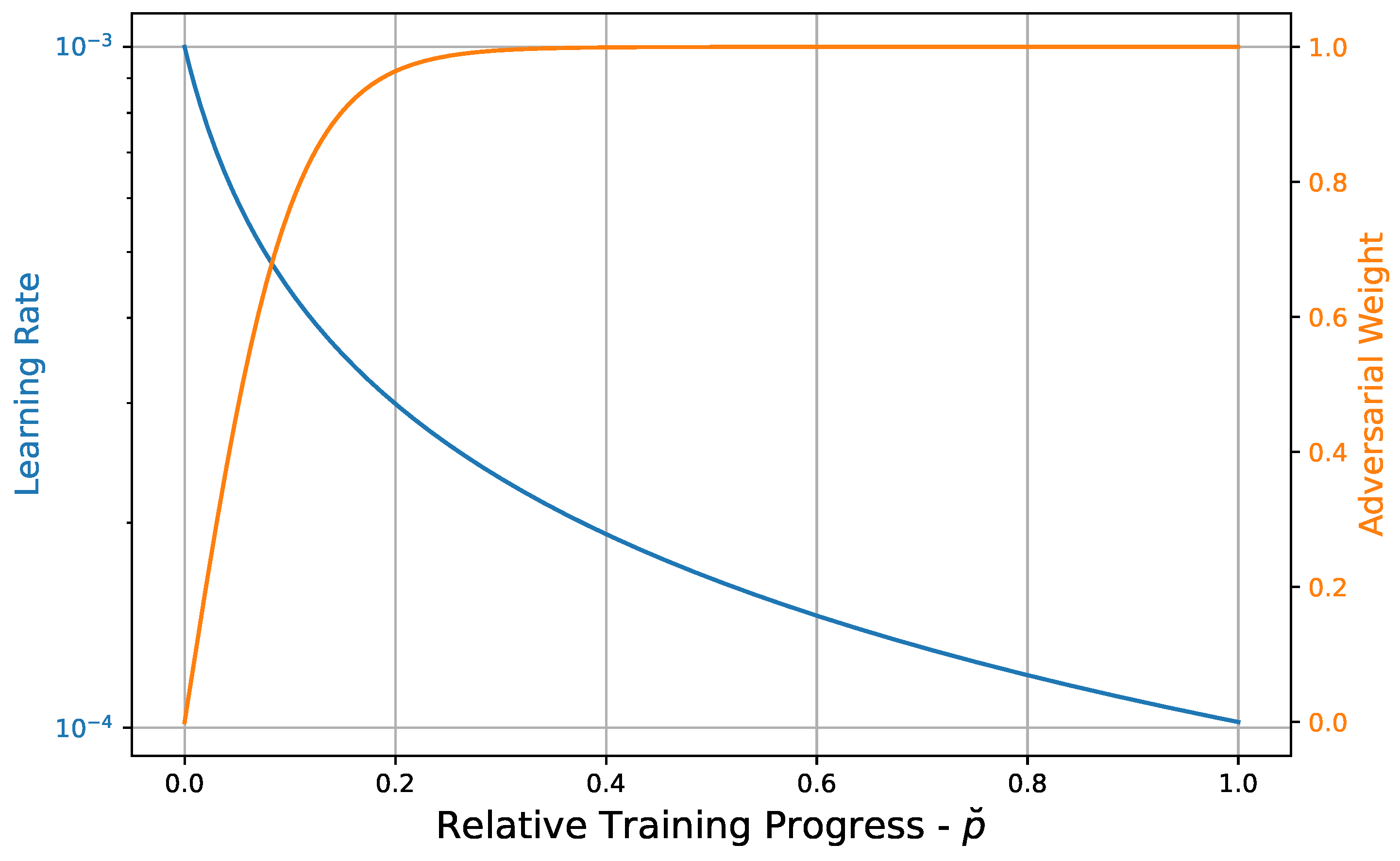
All models are trained using the Adam optimizer. For the non-adaptive baseline, models are trained with a fixed learning rate ( for ResNet architectures and for ViT-Tiny) and no weight decay. For all domain adaptation methods, a dynamic scheduling scheme is employed for both the learning rate and the adversarial weighting parameter to promote stable convergence and mitigate early overfitting of the discriminator. Both hyperparameters are updated according to the relative training progress , according to the following expressions:
where the schedule hyper-hyperparameters are updated to , , and (see Figure 9).
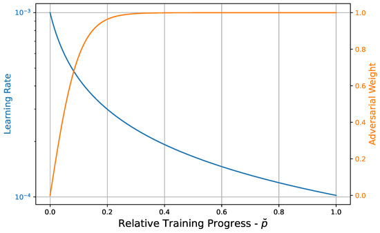
Figure 9.
Dynamic scheduling of learning rate and adversarial weighting factor as functions of the relative training progress (horizontal axis, dimensionless, 0–1) and their values in logarithmic scale (vertical axis). Blue: learning rate . Orange: adversarial weight , see Equation (29).
In addition to stratified sampling, the batch size is dynamically adjusted based on the size of the training set (N) in each domain, according to the following empirical rule:
The initial learning rate was empirically tuned for each model, method, and dataset, typically ranging from to . Notably, the first stage of ADDA was trained with a fixed learning rate of . Furthermore, to adapt the pretrained ViT-Tiny architecture for the lower-resolution Digits dataset (), we applied bicubic interpolation to its positional embeddings. This step was necessary to align the spatial dimensions of the pretrained weights (originally for inputs) with the target image size, enabling effective knowledge transfer.
Next, to maintain class balance during model training and evaluation, an initial partition is performed into training (70%), validation (15%), and test (15%) subsets. This process is conducted independently for both the source and target domains. To ensure representative subsets, stratified sampling is applied within each partition, preserving the internal class distributions of each domain. In particular, the independent construction of the validation sets enables consistent and comparable evaluation conditions across domains, which is essential in domain adaptation scenarios where distributional shifts may introduce evaluation bias.
The lower and upper bounds were established empirically. The lower bound ensures the existence of at least 10 mini-batches per epoch, contributing to optimization stability and preventing prohibitively long training times on small datasets. Conversely, the upper bound avoids excessively large batches that could destabilize learning or exceed GPU memory capacity. This configuration strikes an effective trade-off between gradient stability and computational efficiency, especially when handling domains of different sizes.
It is important to note that, since both dataset partitioning and batch size are determined by the number of available samples in each domain, the number of training instances per epoch is not the same across domains. This asymmetry reflects the inherent scale differences between datasets and allows each domain to contribute proportionally to the learning process without enforcing artificial uniformity.
For all experiments, the kernel bandwidth parameter used in the estimation of Rényi’s quadratic entropy was adaptively determined for each training batch using the median heuristic. This common practice involves setting as the square root of the median of all pairwise squared Euclidean distances within the combined source and target feature batch, as follows [83]:
This data-driven approach automates a critical hyperparameter, ensuring that the kernel’s scale is appropriately tailored to the feature distribution, which enhances the stability and effectiveness of the alignment process across domains.
Moreover, to qualitatively assess the discriminative capacity of the learned features, we apply dimensionality reduction using UMAP, leveraging the GPU-accelerated cuML implementation. Unless otherwise stated, the default parameters are set as follows: n_components = 2, n_neighbors = 80, and random_state = 42. Prior to projection, features are normalized with MinMaxScaler, which facilitates visual inspection of inter-class and inter-domain separability in the latent space. Also, we employ the GradCAM++ technique via the torchcam library to visualize class-specific attention regions within the input images. Representative samples for each class are selected from both source and target domains, and the last convolutional layer of the feature extractor is designated as the target layer. The resulting attention masks are normalized and overlaid on the corresponding images, offering a qualitative perspective on the spatial focus of the model during classification.
Our experiments were conducted on the Google Colab platform, leveraging a high-performance instance equipped with a NVIDIA (Santa Clara, CA, USA) A100 GPU (40.0 GB of VRAM), 83.5 GB of system RAM, and 235.7 GB of disk storage. For full reproducibility, we set a global random seed of 42 across Python, NumPy 2.0.2, and PyTorch (for both CPU and CUDA) and configured the cuDNN backend to use deterministic algorithms, ensuring consistent results from GPU computations. The development environment was based on Python 3.11.11, using PyTorch 2.1.2 for model training, cuML 25.02.01 for GPU-accelerated UMAP visualization, and torchcam 0.4.0 for GradCAM++. All source code and datasets are publicly available at: https://github.com/Daprosero/Domain_Adaptation (accessed on 4 July 2025).
4. Results and Discussion
4.1. Domain Adaption Results
A fundamental objective in domain adaptation is to learn representations that remain invariant under distributional shifts between domains, commonly referred to as covariate shift. A model’s ability to mitigate this challenge is directly reflected in its accuracy on the target domain. To evaluate CREDA’s performance quantitatively, we conducted experiments on three widely adopted benchmark datasets using various backbone architectures.
In the digit adaptation tasks (see Table 6), CREDA demonstrates state-of-the-art performance, achieving the highest average accuracy with both ResNet-18 (62.65%) and ResNet-50 (64.07%) backbones. It performs exceptionally well in challenging tasks such as M→U (achieving up to 91.77% with ResNet-50), characterized by significant visual disparities. A noteworthy observation arises with the ViT-Tiny backbone. Here, conventional adversarial methods like DANN, ADDA, and CDAN+E experience a significant performance collapse, falling well below the source-only Baseline. This suggests that the dynamics of adversarial training may be unstable or less compatible with the global, patch-based feature space learned by Transformers, in contrast to the hierarchical features of CNNs. Nevertheless, CREDA is markedly less affected by this architectural shift. While the Baseline achieves the top rank in this specific instance, CREDA’s performance (47.23%) remains highly competitive and substantially surpasses other adaptation methods, highlighting its greater architectural robustness.

Table 6.
Accuracy (%) on Digits for unsupervised domain adaptation using different backbone architectures.
Similarly, on the ImageCLEF-DA dataset (see Table 7), CREDA’s superiority is even more pronounced. It consistently achieves top-tier results, securing the highest average accuracy across all three backbones. Critically, with the ViT-Tiny backbone, CREDA (82.41%) is the only adaptation method to decisively outperform the strong Baseline model (80.19%). This again contrasts sharply with other adversarial methods, which either lag or perform on par with the Baseline. This reinforces the hypothesis that CREDA’s Rényi entropy-based regularization offers a more stable and effective path to domain alignment than the adversarial objectives of its counterparts, particularly when paired with Transformer architectures. These results suggest that our method more effectively balances domain alignment and the preservation of class discriminability.

Table 7.
Accuracy (%) on ImageCLEF-DA for unsupervised domain adaptation using different backbone architectures.
Lastly, on the Office-31 benchmark (see Table 8), CREDA confirms its superiority by achieving the highest average accuracy across all backbones, peaking at 92.96% with ResNet-50. The trend of architectural robustness continues, as CREDA again outperforms all other methods with ViT-Tiny, achieving an average accuracy of 89.31% against the Baseline’s 85.46%. The fragility of other methods is particularly evident here, with DANN, ADDA, and CDAN+E suffering catastrophic performance drops (e.g., 20.14% for DANN on D → A), rendering them less effective than a simple no-adaptation approach. This consistently demonstrates CREDA’s ability not only to adapt effectively but also to generalize its mechanism across fundamentally different architectural paradigms, from convolutional to attention-based models.

Table 8.
Accuracy (%) on Office-31 for unsupervised domain adaptation using different backbone architectures.
To provide a robust statistical assessment of our method’s consistency and superiority, we conducted a Friedman test on the accuracy ranks across all nine experimental configurations (three datasets × three backbones). The test revealed a statistically significant difference among the methods’ performances (, ), thus allowing us to reject the null hypothesis that all approaches perform equally. This result provides strong evidence that the observed differences in performance are not due to random chance.
Table 9 shows that CREDA achieves the best (lowest) average rank of 1.22. Furthermore, its performance stability is underscored by a remarkably low standard deviation (), the lowest among all evaluated methods. This indicates that CREDA consistently ranked at or near the top, irrespective of the dataset or backbone architecture. In contrast, methods like the Baseline () exhibit much higher variance, suggesting their performance is less stable across different settings. This statistical validation robustly confirms that CREDA’s leading performance is not an artifact of specific experimental conditions but rather a consistent and significant advantage across a diverse range of domains and model architectures, including the challenging Transformer-based setups where other adaptation techniques falter.

Table 9.
Average classification rank of all methods across datasets and model architectures. Ranks are assigned per block (row) based on average accuracy. The final row presents the mean rank ± standard deviation for each method. The Friedman test confirms a significant difference in performance (, ).
4.2. Interpretability Results
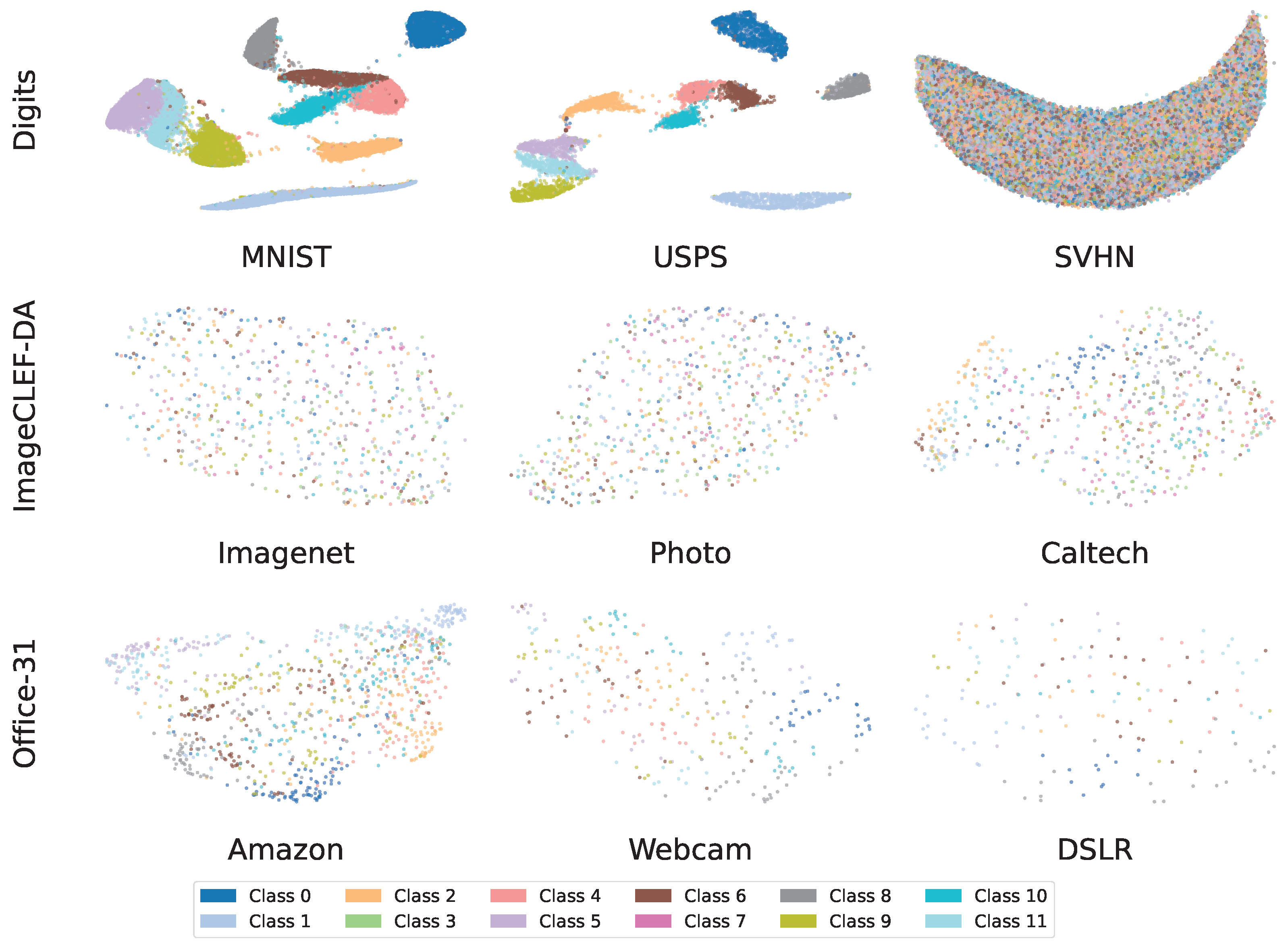
To clarify the reasons for these performance disparities, it is crucial to first examine the inherent complexity of the data domains. Figure 10 presents the 2D UMAP projections of the original feature space, visualized independently for each domain. These plots reveal a fundamental challenge that extends beyond domain shift: the limited class separability within individual domains. This limitation is particularly pronounced in complex datasets such as ImageCLEF-DA and Office-31, where class instances (depicted by distinct colors) exhibit significant entanglement, forming dense and unstructured distributions. Such inherent visual similarity among categories not only complicates classification within the source domain but also serves as a principal source of noisy pseudo-labels in the target domain during unsupervised adaptation. Consequently, a robust domain adaptation strategy must not only align cross-domain distributions but also construct feature representations that enhance inter-class discrimination.
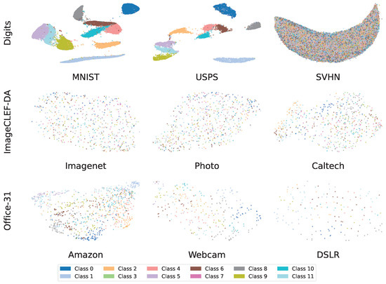
Figure 10.
Two-dimensional UMAP projections of original feature representations before domain adaptation. Rows: evaluated benchmarks. Columns: domains within each benchmark.
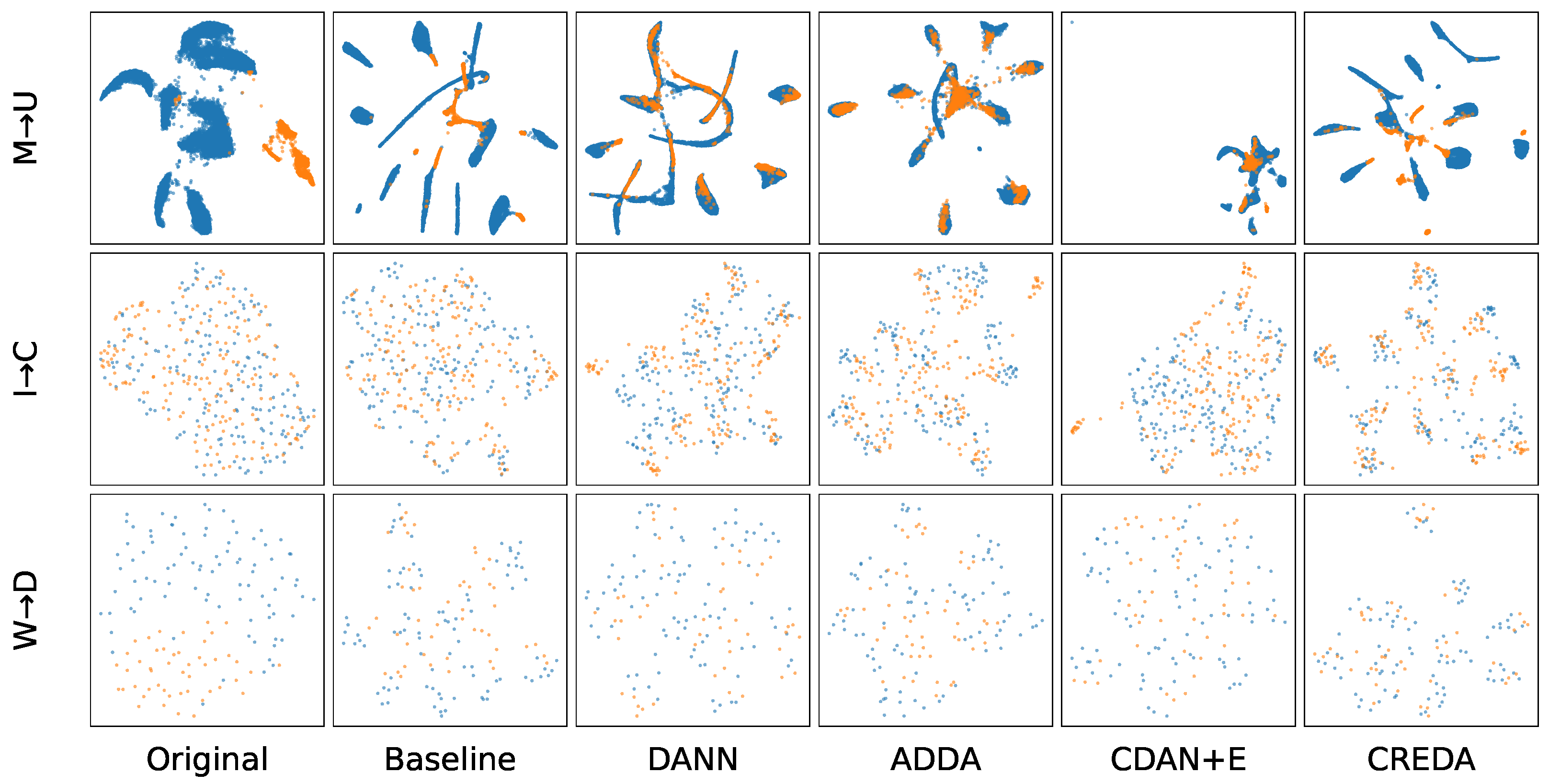
Building upon this analysis, Figure 11 illustrates how different adaptation techniques address these structural challenges, visualized through UMAP projections of the learned latent spaces. The first column depicts the initial state prior to training, highlighting both the pronounced domain gap (e.g., M → U) and the poor semantic organization (e.g., I → C). The Baseline model, trained exclusively on source data, fails to bridge this gap, maintaining a clear division between domains. In contrast, adversarial methods like DANN and ADDA achieve some domain alignment, but often at the expense of class coherence, resulting in fragmented (as seen in M → U) and disordered representations across all tasks. While CDAN+E introduces a modest improvement in structural consistency, significant inter-class dispersion remains. Ultimately, CREDA yields a markedly superior configuration: it not only facilitates seamless domain integration—evidenced by the homogeneous blending of source and target samples—but also preserves (M → U) and, notably, enhances (I → C, W → D) class-wise separability, as demonstrated by the emergence of compact, well-defined clusters from initially unstructured feature spaces. This outcome provides a visual explanation for CREDA’s superior quantitative performance, indicating its ability to balance the removal of spurious domain-specific cues with the preservation and recovery of underlying semantic structure.
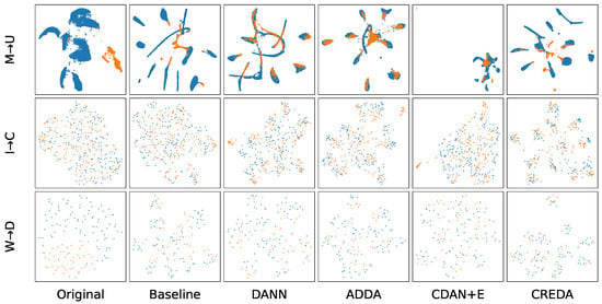
Figure 11.
UMAP projections of the learned feature representations across domain adaptation methods, with the source domain shown in blue and the target domain in orange. Rows: datasets used in the evaluation. Columns: compared adaptation models.
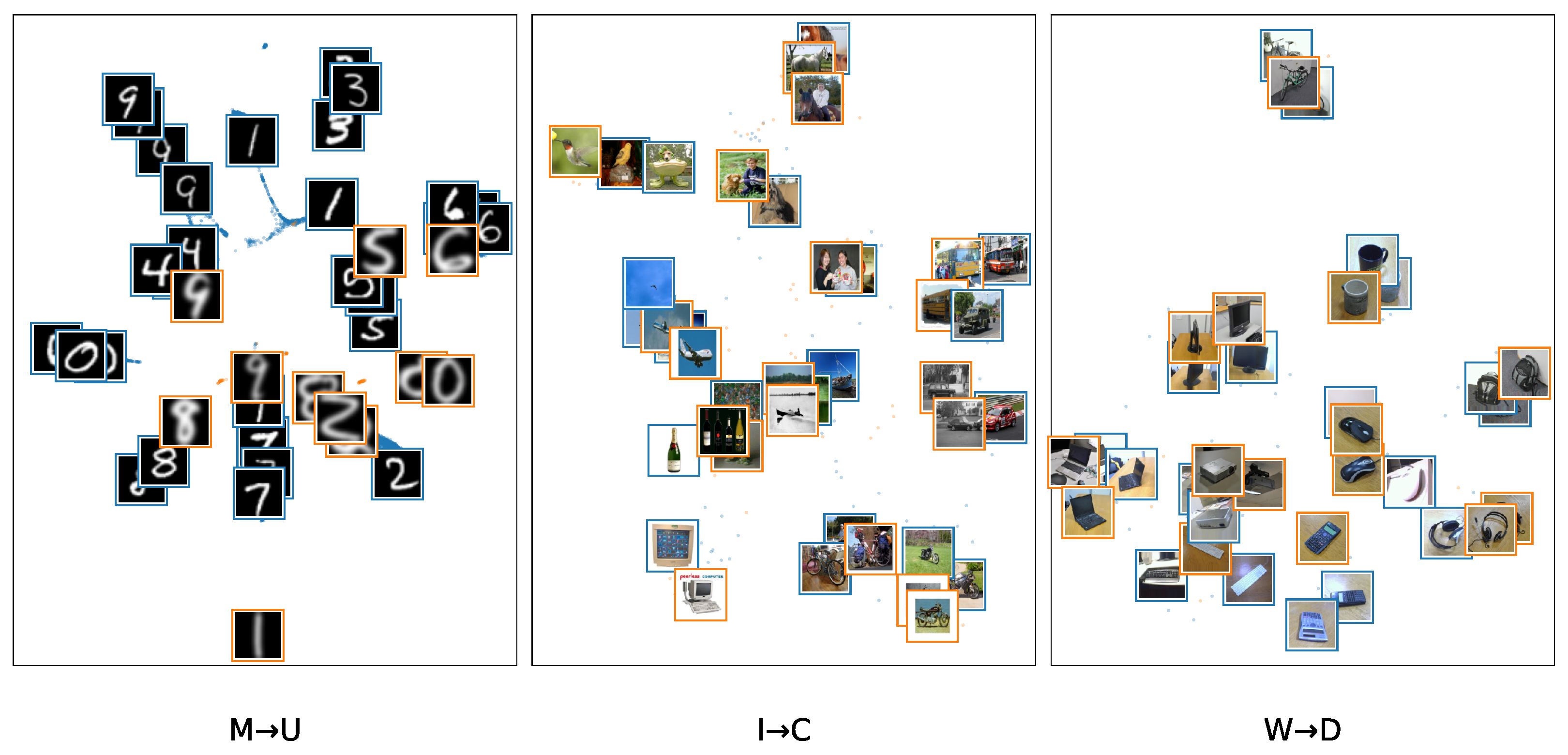
Having established CREDA’s capacity to address covariate shift, we next assess whether the learned representations preserve semantic coherence under concept shift, where object appearance changes substantially across domains. In this context, Figure 12 presents UMAP projections with embedded images to qualitatively examine the model’s ability to cluster semantically related concepts.
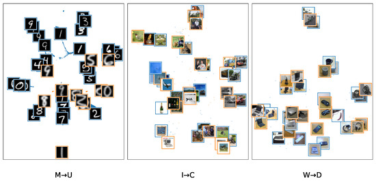
Figure 12.
UMAP projections of learned feature representations under the CREDA model, with input images overlaid, where source domain samples appear in blue and target domain samples in orange. Left: Digits. Middle: ImageCLEF-DA. Right: Office-31.
The results indicate that CREDA learns a semantically rich feature space that transcends superficial variability. For instance, in the M → U task, the model accurately groups digits despite substantial stylistic differences, as seen in the clusters corresponding to digits 6, 0, and 4. In the I → C task, it successfully groups semantically similar but visually diverse objects, forming distinct clusters for categories like airplanes and bottles despite variations in perspective and background. Similarly, in the W → D task, objects such as keyboards and mugs are grouped according to their semantic identity, overcoming differences in image quality. Altogether, these visualizations demonstrate that CREDA not only aligns domains but also constructs a feature space in which proximity reflects conceptual similarity—an essential attribute for robust generalization in real-world applications.
Finally, to reinforce the model’s reliability, it is essential not only to demonstrate high accuracy and semantic coherence, but also to ensure that its predictions are grounded in interpretable reasoning. In other words, it must be verified that decisions are driven by relevant visual cues rather than spurious correlations.
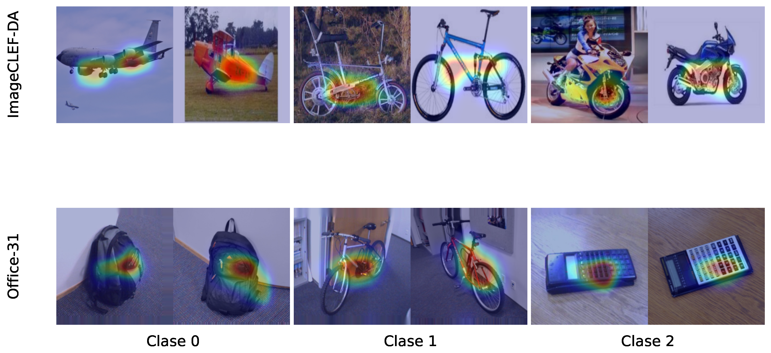
To address this, we employ Grad-CAM++, with the results shown in Figure 13. The heatmaps reveal strong semantic consistency: regardless of the domain, the model focuses attention on canonical and representative regions of the object, such as the face in a portrait or the main structural components of a vehicle. This confirms that CREDA does not rely on superficial distribution alignment, but rather performs deep and meaningful semantic knowledge transfer. These findings not only enhance trust in the model’s predictions but also establish CREDA as a transparent and robust solution for domain adaptation, strengthening the interpretability and reliability of its outputs.

Figure 13.
Class-wise visual explanations under the CREDA model. Each pair of images shows the source domain on the left and the corresponding target domain on the right. Heatmaps highlight the most salient regions contributing to the predicted class.
4.3. Training and Inference Time Analysis
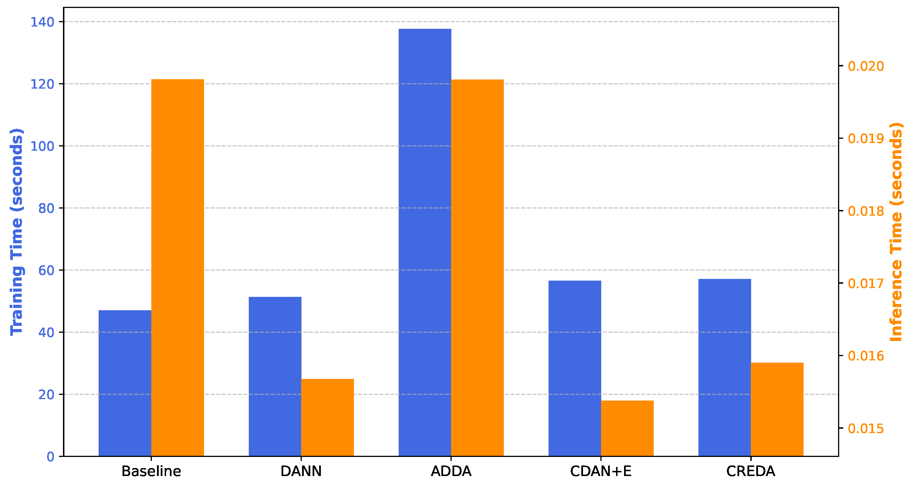
To assess practical viability, we measured training and inference time on the M → S task, selected for being the most extensive dataset combination. ResNet-50 was used as the feature extractor due to its higher computational demand relative to the other backbones, offering a conservative estimate of resource requirements. As shown in Figure 14, ADDA incurs the highest training cost due to its two-phase architecture, whereas single-stage methods (DANN, CDAN+E, and CREDA) introduce only a marginal overhead compared to the Baseline. Regarding inference, all adapted models were highly efficient. Notably, DANN, CDAN+E, and CREDA demonstrated slightly faster inference than the Baseline and ADDA, potentially because the learned domain-invariant features streamline the forward pass. This analysis confirms that CREDA offers a compelling trade-off, delivering superior accuracy with a manageable training cost while maintaining efficient inference speeds suitable for real-world deployment.

Figure 14.
Training and inference time comparison across domain adaptation methods. The left axis shows training time per epoch, while the right axis shows average inference time per sample.
4.4. Limitations
Despite the robust performance of the CREDA framework on unsupervised domain adaptation tasks, several limitations must be acknowledged. These, in turn, present pertinent avenues for future research. While CREDA demonstrates superior performance even when implemented on deeper CNNs or ViT-based architectures, a comprehensive investigation is required to fully characterize its scaling properties in large-scale or multi-resolution contexts. Secondly, a singular hyperparameter tuning strategy was employed across all tasks, thereby precluding domain-pair-specific optimization. The incorporation of automated search schemes for adaptation could potentially enhance performance and generalization, albeit at an increased computational cost [84]. Thirdly, the combination of the classification loss and the Rényi divergence-based regularization relies on a static weighting coefficient. Exploring an adaptive normalization method for the loss functions could foster more stable training dynamics by balancing the magnitudes of the gradients. Moreover, as the regularizer is contingent upon kernel-based estimations, the model’s performance exhibits sensitivity to the kernel bandwidth. Although the median heuristic was employed to set this bandwidth at each training step, such a data-driven strategy may not generalize optimally across all domain pairs or distributions, warranting further exploration of adaptive kernel selection schemes.
In particular, CREDA’s performance reveals its limitations, particularly in scenarios with extreme domain shifts. Quantitatively, the method’s effectiveness degrades most significantly on adaptation tasks involving the SVHN (S) dataset, such as M→S and U→S, where it achieves its lowest absolute accuracies (see Table 6). The severe performance drop of the source-only Baseline on these tasks confirms that the domain gap—transitioning from clean, centered digits to cluttered, real-world house numbers—is exceptionally large. This suggests that CREDA, while robust, struggles when the target domain introduces fundamental changes in image composition, including complex backgrounds, color variations, and distracting neighboring elements, which are not present in the source domain. Qualitatively, this failure mode can be attributed to the quality of the initial pseudo-labels. In extreme-shift scenarios, the classifier, trained only on source data, produces target pseudo-labels that are either confidently wrong or universally low-confidence. For instance, an SVHN digit ‘1’ with artifacts may be confidently misclassified as a ‘7’, or a ‘3’ with poor lighting as an ‘8’. While our entropy-based weighting is designed to mitigate noise, it cannot overcome a situation where the initial class-conditional signal is systematically corrupted. Consequently, CREDA’s primary limitation arises when the domain gap is so vast that it prevents the model from forming a reasonably accurate initial estimate of the target domain’s semantic structure, thereby undermining the effectiveness of the class-conditional alignment mechanism.
5. Conclusions
This work introduced a novel domain adaptation framework, termed Conditional Rényi -Entropy Domain Adaptation (CREDA), a deep learning-based strategy integrating kernel-based conditional alignment from a matrix-based formulation of Rényi’s quadratic entropy. CREDA is structured around three key components. First, a deep feature extractor is used to learn domain-invariant representations by leveraging labeled source data and unlabeled target data. Second, an entropy-weighted strategy attenuates the influence of low-confidence pseudo-labels, thereby enhancing robustness in ambiguous regions. Third, a class-conditional alignment loss, expressed as a Rényi divergence, is introduced to promote semantic consistency across domains within the latent representation space. In contrast to supervised or semi-supervised approaches, the proposed method does not require labels in the target domain, making it particularly suitable for scenarios where annotation is costly or unavailable. Moreover, our class-wise alignment is formulated in a non-parametric and differentiable manner by leveraging kernel-based information potentials, enabling the preservation of semantic structure across domains.
Experimental results across diverse visual adaptation scenarios demonstrate that CREDA consistently outperforms conventional methods such as DANN, ADDA, and CDAN+E in terms of predictive accuracy, representational quality, and interpretability. In particular, CREDA achieves the highest average accuracy across all datasets and architectures, with noticeable improvements when using deeper CNNs (ResNet-50) and attention-based models (ViT-Tiny). While most adversarial approaches experience performance degradation in these settings, CREDA remains robust and effective, as evidenced by the results presented in this study. Notably, CREDA maintains class separability even under complex distribution shifts and when the predicted labels in the target domain exhibit low confidence. The integration of UMAP- and GradCAM++-based visualizations offers valuable insights into the learned representations, reinforcing its applicability in real-world settings where traceability and semantic coherence are critical. From an implementation standpoint, CREDA does not require modifications to the classification loss function. Its confidence-aware weighting scheme and class-conditional regularization enhance robustness to pseudo-label noise and class imbalance. Moreover, its modular architecture facilitates seamless integration into existing deep learning pipelines.
As future work, we aim to test CREDA on larger-scale datasets. Also, we plan to extend CREDA to multi-source and continual domain adaptation settings, where domain shifts occur either simultaneously or sequentially. Attention-based class-conditioned alignment across multiple source domains has been shown to mitigate negative transfer and effectively address class imbalance [85]. Second, we plan to incorporate class-conditional kernel alignment and attention-guided feature disentanglement to improve both interpretability and discriminative alignment, particularly in contexts characterized by subtle inter-class distinctions or limited labeled data. Additionally, exploring temporal or streaming variants of CREDA could prove beneficial in online adaptation scenarios, where data arrives sequentially and models must adapt incrementally. Recent advances in attention-aware class-conditioned alignment suggest that these mechanisms yield robust feature representations and highlight relevant discriminative regions in multi-source adaptation [86]. Finally, while CREDA was conceived for the standard unsupervised adaptation setting, its extension to more challenging scenarios, such as few-shot or source-free adaptation, remains uninvestigated [87]. Addressing these limitations would not only enhance the robustness of the proposed framework but also broaden its applicability to more complex transfer learning problems.
Author Contributions
Conceptualization, D.A.P.-R., A.M.Á.-M. and G.C.-D.; data curation, D.A.P.-R.; methodology, D.A.P.-R., A.M.Á.-M. and G.C.-D.; project administration, A.M.Á.-M.; supervision, A.M.Á.-M. and G.C.-D.; resources, D.A.P.-R. and A.M.Á.-M. All authors have read and agreed to the published version of the manuscript.
Funding
Under grants provived by the project: “Prototipo funcional de lengua electrónica para la identificación de sabores en cacao fino de origen colombiano”, funded by Minciencias-82729-ICETEX 2022-0740 and Casa Luker. Also, A.M. Alvarez thanks the following project: “Aprendizaje de máquina cuántico utilizando espines electrónicos”, Hermes-62836, funded by Universidad Nacional de Colombia and Universidad de Caldas.
Data Availability Statement
The publicly available dataset analyzed in this study and our Python codes can be found at https://github.com/Daprosero/Domain_Adaptation (accessed on 4 July 2025).
Conflicts of Interest
The authors declare no conflicts of interest.
References
- Lu, X.; Yao, X.; Jiang, Q.; Shen, Y.; Xu, F.; Zhu, Q. Remaining useful life prediction model of cross-domain rolling bearing via dynamic hybrid domain adaptation and attention contrastive learning. Comput. Ind. 2025, 164, 104172. [Google Scholar] [CrossRef]
- Wu, H.; Shi, C.; Yue, S.; Zhu, F.; Jin, Z. Domain Adaptation Network Based on Multi-Level Feature Alignment Constraints for Cross Scene Hyperspectral Image Classification. Knowl.-Based Syst. 2025, 113972. [Google Scholar] [CrossRef]
- Huang, X.Y.; Chen, S.Y.; Wei, C.S. Enhancing Low-Density EEG-Based Brain-Computer Interfacing With Similarity-Keeping Knowledge Distillation. IEEE Trans. Emerg. Top. Comput. Intell. 2023, 8, 1156–1166. [Google Scholar] [CrossRef]
- Jiang, J.; Zhao, S.; Zhu, J.; Tang, W.; Xu, Z.; Yang, J.; Liu, G.; Xing, T.; Xu, P.; Yao, H. Multi-source domain adaptation for panoramic semantic segmentation. Inf. Fusion 2025, 117, 102909. [Google Scholar] [CrossRef]
- Imtiaz, M.N.; Khan, N. Towards Practical Emotion Recognition: An Unsupervised Source-Free Approach for EEG Domain Adaptation. arXiv 2025, arXiv:2504.03707. [Google Scholar]
- Wang, J.; Lan, C.; Liu, C.; Ouyang, Y.; Qin, T.; Lu, W.; Chen, Y.; Zeng, W.; Yu, P.S. Generalizing to unseen domains: A survey on domain generalization. IEEE Trans. Knowl. Data Eng. 2022, 35, 8052–8072. [Google Scholar] [CrossRef]
- Galappaththige, C.J.; Baliah, S.; Gunawardhana, M.; Khan, M.H. Towards generalizing to unseen domains with few labels. In Proceedings of the IEEE/CVF Conference on Computer Vision and Pattern Recognition, Seattle, WA, USA, 16–22 June 2024; pp. 23691–23700. [Google Scholar]
- Zhu, H.; Bai, J.; Li, N.; Li, X.; Liu, D.; Buckeridge, D.L.; Li, Y. FedWeight: Mitigating covariate shift of federated learning on electronic health records data through patients re-weighting. npj Digit. Med. 2025, 8, 286. [Google Scholar] [CrossRef]
- Li, L.; Zhang, X.; Liang, J.; Chen, T. Addressing Domain Shift via Imbalance-Aware Domain Adaptation in Embryo Development Assessment. arXiv 2025, arXiv:2501.04958. [Google Scholar] [CrossRef]
- Yuksel, G.; Kamps, J. Interpretability Analysis of Domain Adapted Dense Retrievers. arXiv 2025, arXiv:2501.14459. [Google Scholar]
- Adachi, K.; Yamaguchi, S.; Kumagai, A.; Hamagami, T. Test-time Adaptation for Regression by Subspace Alignment. arXiv 2024, arXiv:2410.03263. [Google Scholar] [CrossRef]
- Zhang, G.; Zhou, T.; Cai, Y. CORAL-based Domain Adaptation Algorithm for Improving the Applicability of Machine Learning Models in Detecting Motor Bearing Failures. J. Comput. Methods Eng. Appl. 2023, 3, 1–17. [Google Scholar] [CrossRef]
- Wang, J.; Feng, W.; Chen, Y.; Yu, H.; Huang, M.; Yu, P.S. Visual domain adaptation with manifold embedded distribution alignment. In Proceedings of the 26th ACM International Conference on Multimedia, Seoul, Republic of Korea, 22–26 October 2018; pp. 402–410. [Google Scholar]
- Yun, K.; Satou, H. GAMA++: Disentangled Geometric Alignment with Adaptive Contrastive Perturbation for Reliable Domain Transfer. arXiv 2025, arXiv:2505.15241. [Google Scholar]
- Sanodiya, R.K.; Yao, L. A subspace based transfer joint matching with Laplacian regularization for visual domain adaptation. Sensors 2020, 20, 4367. [Google Scholar] [CrossRef]
- Wei, F.; Xu, X.; Jia, T.; Zhang, D.; Wu, X. A multi-source transfer joint matching method for inter-subject motor imagery decoding. IEEE Trans. Neural Syst. Rehabil. Eng. 2023, 31, 1258–1267. [Google Scholar] [CrossRef]
- Battu, R.S.; Agathos, K.; Monsalve, J.M.L.; Worden, K.; Papatheou, E. Combining transfer learning and numerical modelling to deal with the lack of training data in data-based SHM. J. Sound Vib. 2025, 595, 118710. [Google Scholar] [CrossRef]
- Yano, M.O.; Figueiredo, E.; da Silva, S.; Cury, A. Foundations and applicability of transfer learning for structural health monitoring of bridges. Mech. Syst. Signal Process. 2023, 204, 110766. [Google Scholar] [CrossRef]
- Liang, S.; Li, L.; Zu, W.; Feng, W.; Hang, W. Adaptive deep feature representation learning for cross-subject EEG decoding. BMC Bioinform. 2024, 25, 393. [Google Scholar] [CrossRef]
- Chen, G.; Xiang, D.; Liu, T.; Xu, F.; Fang, K. Deep discriminative domain adaptation network considering sampling frequency for cross-domain mechanical fault diagnosis. Expert Syst. Appl. 2025, 280, 127296. [Google Scholar] [CrossRef]
- Wei, G.; Lan, C.; Zeng, W.; Chen, Z. Metaalign: Coordinating domain alignment and classification for unsupervised domain adaptation. In Proceedings of the IEEE/CVF Conference on Computer Vision and Pattern Recognition, Nashville, TN, USA, 20–25 June 2021; pp. 16643–16653. [Google Scholar]
- Zhang, Y.; Wang, X.; Liang, J.; Zhang, Z.; Wang, L.; Jin, R.; Tan, T. Free lunch for domain adversarial training: Environment label smoothing. arXiv 2023, arXiv:2302.00194. [Google Scholar] [CrossRef]
- Lu, M.; Huang, Z.; Zhao, Y.; Tian, Z.; Liu, Y.; Li, D. DaMSTF: Domain adversarial learning enhanced meta self-training for domain adaptation. arXiv 2023, arXiv:2308.02753. [Google Scholar]
- Wu, Y.; Spathis, D.; Jia, H.; Perez-Pozuelo, I.; Gonzales, T.I.; Brage, S.; Wareham, N.; Mascolo, C. Udama: Unsupervised domain adaptation through multi-discriminator adversarial training with noisy labels improves cardio-fitness prediction. In Proceedings of the Machine Learning for Healthcare Conference, New York, NY, USA, 11–12 August 2023; PMLR: Cambridge, MA, USA, 2023; pp. 863–883. [Google Scholar]
- Mehra, A.; Kailkhura, B.; Chen, P.Y.; Hamm, J. Understanding the limits of unsupervised domain adaptation via data poisoning. Adv. Neural Inf. Process. Syst. 2021, 34, 17347–17359. [Google Scholar]
- Zhu, Y.; Zhuang, F.; Wang, J.; Chen, J.; Shi, Z.; Wu, W.; He, Q. Multi-representation adaptation network for cross-domain image classification. Neural Netw. 2019, 119, 214–221. [Google Scholar] [CrossRef] [PubMed]
- Madadi, Y.; Seydi, V.; Sun, J.; Chaum, E.; Yousefi, S. Stacking Ensemble Learning in Deep Domain Adaptation for Ophthalmic Image Classification. In Ophthalmic Medical Image Analysis: Proceedings of the 8th International Workshop, OMIA 2021, Held in Conjunction with MICCAI 2021, Strasbourg, France, 27 September 2021, Proceedings 8; Springer: Berlin/Heidelberg, Germany, 2021; pp. 168–178. [Google Scholar]
- Zhu, Y.; Zhuang, F.; Wang, J.; Ke, G.; Chen, J.; Bian, J.; Xiong, H.; He, Q. Deep subdomain adaptation network for image classification. IEEE Trans. Neural Netw. Learn. Syst. 2020, 32, 1713–1722. [Google Scholar] [CrossRef]
- Li, X.; Chen, H.; Li, S.; Wei, D.; Zou, X.; Si, L.; Shao, H. Multi-kernel weighted joint domain adaptation network for cross-condition fault diagnosis of rolling bearings. Reliab. Eng. Syst. Saf. 2025, 261, 111109. [Google Scholar] [CrossRef]
- Xiao, L.; Xu, J.; Zhao, D.; Wang, Z.; Wang, L.; Nie, Y.; Dai, B. Self-supervised domain adaptation with consistency training. In Proceedings of the 2020 25th International Conference on Pattern Recognition (ICPR), Milan, Italy, 10–15 January 2021; IEEE: Piscataway, NJ, USA, 2021; pp. 6874–6880. [Google Scholar]
- Wang, R.; Wu, Z.; Weng, Z.; Chen, J.; Qi, G.J.; Jiang, Y.G. Cross-domain contrastive learning for unsupervised domain adaptation. IEEE Trans. Multimed. 2022, 25, 1665–1673. [Google Scholar] [CrossRef]
- Kang, G.; Jiang, L.; Yang, Y.; Hauptmann, A.G. Contrastive adaptation network for unsupervised domain adaptation. In Proceedings of the IEEE/CVF Conference on Computer Vision and Pattern Recognition, Long Beach, CA, USA, 15–20 June 2019; pp. 4893–4902. [Google Scholar]
- Jia, M.; Tang, L.; Chen, B.C.; Cardie, C.; Belongie, S.; Hariharan, B.; Lim, S.N. Visual prompt tuning. In Proceedings of the European Conference on Computer Vision, Tel Aviv, Israel, 23–27 October 2022; Springer: Cham, Switzerland, 2022; pp. 709–727. [Google Scholar]
- Kirillov, A.; Mintun, E.; Ravi, N.; Mao, H.; Rolland, C.; Gustafson, L.; Xiao, T.; Whitehead, S.; Berg, A.C.; Lo, W.Y.; et al. Segment anything. In Proceedings of the IEEE/CVF International Conference on Computer Vision, Paris, France, 1–6 October 2023; pp. 4015–4026. [Google Scholar]
- Chen, H.; Chen, H.; Zhao, Z.; Han, K.; Zhu, G.; Zhao, Y.; Du, Y.; Xu, W.; Shi, Q. An overview of domain-specific foundation model: Key technologies, applications and challenges. arXiv 2024, arXiv:2409.04267. [Google Scholar] [CrossRef]
- Chen, L.; Chen, H.; Wei, Z.; Jin, X.; Tan, X.; Jin, Y.; Chen, E. Reusing the task-specific classifier as a discriminator: Discriminator-free adversarial domain adaptation. In Proceedings of the IEEE/CVF Conference on Computer Vision and Pattern Recognition, New Orleans, LA, USA, 18–24 June 2022; pp. 7181–7190. [Google Scholar]
- Xiao, R.; Liu, Z.; Wu, B. Teacher-student competition for unsupervised domain adaptation. In Proceedings of the 2020 25th International Conference on Pattern Recognition (ICPR), Milan, Italy, 10–15 January 2021; IEEE: Piscataway, NJ, USA, 2021; pp. 8291–8298. [Google Scholar]
- Choi, E.; Rodriguez, J.; Young, E. An In-Depth Analysis of Adversarial Discriminative Domain Adaptation for Digit Classification. arXiv 2024, arXiv:2412.19391. [Google Scholar] [CrossRef]
- Lu, W.; Luu, R.K.; Buehler, M.J. Fine-tuning large language models for domain adaptation: Exploration of training strategies, scaling, model merging and synergistic capabilities. npj Comput. Mater. 2025, 11, 84. [Google Scholar] [CrossRef]
- Kumar, A.; Raghunathan, A.; Jones, R.; Ma, T.; Liang, P. Fine-tuning can distort pretrained features and underperform out-of-distribution. arXiv 2022, arXiv:2202.10054. [Google Scholar] [CrossRef]
- Liu, Y.; Wong, W.; Liu, C.; Luo, X.; Xu, Y.; Wang, J. Mutual Learning for SAM Adaptation: A Dual Collaborative Network Framework for Source-Free Domain Transfer. In Proceedings of the 42nd International Conference on Machine Learning (ICML), Vancouver, BC, Canada, 13–19 July 2025. Poster presentation. [Google Scholar]
- Gao, Y.; Baucom, B.; Rose, K.; Gordon, K.; Wang, H.; Stankovic, J.A. E-ADDA: Unsupervised Adversarial Domain Adaptation Enhanced by a New Mahalanobis Distance Loss for Smart Computing. In Proceedings of the 2023 IEEE International Conference on Smart Computing (SMARTCOMP), Nashville, TN, USA, 26–30 June 2023; IEEE: Piscataway, NJ, USA, 2023; pp. 172–179. [Google Scholar]
- Dan, J.; Jin, T.; Chi, H.; Dong, S.; Xie, H.; Cao, K.; Yang, X. Trust-aware conditional adversarial domain adaptation with feature norm alignment. Neural Netw. 2023, 168, 518–530. [Google Scholar] [CrossRef] [PubMed]
- Rao, K.; Harris, C.; Irpan, A.; Levine, S.; Ibarz, J.; Khansari, M. Rl-cyclegan: Reinforcement learning aware simulation-to-real. In Proceedings of the IEEE/CVF Conference on Computer Vision and Pattern Recognition, Seattle, WA, USA, 13–19 June 2020; pp. 11157–11166. [Google Scholar]
- Tang, P.; Peng, L.; Yan, R.; Shi, H.; Yao, G.; Liu, C.; Li, J.; Zhang, Y. Domain adaptation via mutual information maximization for handwriting recognition. In Proceedings of the ICASSP 2022-2022 IEEE International Conference on Acoustics, Speech and Signal Processing (ICASSP), Singapore, 23–27 May 2022; IEEE: Piscataway, NJ, USA, 2022; pp. 2300–2304. [Google Scholar]
- Saito, K.; Kim, D.; Sclaroff, S.; Darrell, T.; Saenko, K. Semi-supervised domain adaptation via minimax entropy. In Proceedings of the IEEE/CVF International Conference on Computer Vision, Seoul, Republic of Korea, 27 October–2 November 2019; pp. 8050–8058. [Google Scholar]
- Chen, J.; Zhang, Z.; Xie, X.; Li, Y.; Xu, T.; Ma, K.; Zheng, Y. Beyond mutual information: Generative adversarial network for domain adaptation using information bottleneck constraint. IEEE Trans. Med. Imaging 2021, 41, 595–607. [Google Scholar] [CrossRef]
- Chang, W.G.; You, T.; Seo, S.; Kwak, S.; Han, B. Domain-specific batch normalization for unsupervised domain adaptation. In Proceedings of the IEEE/CVF Conference on Computer Vision and Pattern Recognition, Long Beach, CA, USA, 15–20 June 2019; pp. 7354–7362. [Google Scholar]
- Wang, H.; Naidu, R.; Michael, J.; Kundu, S.S. Ss-cam: Smoothed score-cam for sharper visual feature localization. arXiv 2020, arXiv:2006.14255. [Google Scholar]
- Mirkes, E.M.; Bac, J.; Fouché, A.; Stasenko, S.V.; Zinovyev, A.; Gorban, A.N. Domain adaptation principal component analysis: Base linear method for learning with out-of-distribution data. Entropy 2022, 25, 33. [Google Scholar] [CrossRef] [PubMed]
- Jeon, H.; Park, J.; Shin, S.; Seo, J. Stop Misusing t-SNE and UMAP for Visual Analytics. arXiv 2025, arXiv:2506.08725. [Google Scholar] [CrossRef]
- McInnes, L.; Healy, J.; Melville, J. Umap: Uniform manifold approximation and projection for dimension reduction. arXiv 2018, arXiv:1802.03426. [Google Scholar]
- Huang, H.; Wang, Y.; Rudin, C.; Browne, E.P. Towards a comprehensive evaluation of dimension reduction methods for transcriptomic data visualization. Commun. Biol. 2022, 5, 719. [Google Scholar] [CrossRef]
- Wei, G.; Lan, C.; Zeng, W.; Zhang, Z.; Chen, Z. Toalign: Task-oriented alignment for unsupervised domain adaptation. Adv. Neural Inf. Process. Syst. 2021, 34, 13834–13846. [Google Scholar]
- Langbein, S.H.; Koenen, N.; Wright, M.N. Gradient-based Explanations for Deep Learning Survival Models. arXiv 2025, arXiv:2502.04970. [Google Scholar]
- Santos, R.; Pedrosa, J.; Mendonça, A.M.; Campilho, A. Grad-CAM: The impact of large receptive fields and other caveats. Comput. Vis. Image Underst. 2025, 258, 104383. [Google Scholar] [CrossRef]
- Singh, A.K.; Chaudhuri, D.; Singh, M.P.; Chattopadhyay, S. Integrative CAM: Adaptive Layer Fusion for Comprehensive Interpretation of CNNs. arXiv 2024, arXiv:2412.01354. [Google Scholar] [CrossRef]
- Ahmad, J.; Rehman, M.I.U.; ul Islam, M.S.; Rashid, A.; Khalid, M.Z.; Rashid, A. Layer-Wise Relevance Propagation in Large-Scale Neural Networks for Medical Diagnosis. Res. Med. Sci. Rev. 2025, 3, 6–18. [Google Scholar]
- Ding, R.; Liu, J.; Hua, K.; Wang, X.; Zhang, X.; Shao, M.; Chen, Y.; Chen, J. Leveraging data mining, active learning, and domain adaptation for efficient discovery of advanced oxygen evolution electrocatalysts. Sci. Adv. 2025, 11, eadr9038. [Google Scholar] [CrossRef]
- Murphy, K.P. Probabilistic Machine Learning: An Introduction; MIT Press: Cambridge, MA, USA, 2022. [Google Scholar]
- Scholkopf, B.; Smola, A.J. Learning with Kernels: Support Vector Machines, Regularization, Optimization, and Beyond; MIT Press: Cambridge, MA, USA, 2018. [Google Scholar]
- Wilson, A.; Adams, R. Gaussian process kernels for pattern discovery and extrapolation. In Proceedings of the International Conference on Machine Learning, Atlanta, GA, USA, 16–21 June 2013; PMLR: Cambridge, MA, USA, 2013; pp. 1067–1075. [Google Scholar]
- Principe, J.C. Information Theoretic Learning: Renyi’s Entropy and Kernel Perspectives; Springer Science & Business Media: New York, NY, USA, 2010. [Google Scholar]
- Bishop, C.M.; Nasrabadi, N.M. Pattern Recognition and Machine Learning; Springer: New York, NY, USA, 2006; Volume 4. [Google Scholar]
- Silverman, B.W. Density Estimation for Statistics and Data Analysis; Routledge: London, UK, 2018. [Google Scholar]
- Xu, J.W.; Paiva, A.R.; Park, I.; Principe, J.C. A reproducing kernel Hilbert space framework for information-theoretic learning. IEEE Trans. Signal Process. 2008, 56, 5891–5902. [Google Scholar] [CrossRef]
- Bromiley, P. Products and convolutions of Gaussian probability density functions. Tina-Vis. Memo 2003, 3, 1. [Google Scholar]
- Giraldo, L.G.S.; Rao, M.; Principe, J.C. Measures of entropy from data using infinitely divisible kernels. IEEE Trans. Inf. Theory 2014, 61, 535–548. [Google Scholar] [CrossRef]
- Giraldo, L.G.S.; Principe, J.C. Information theoretic learning with infinitely divisible kernels. arXiv 2013, arXiv:1301.3551. [Google Scholar] [CrossRef]
- Hatefi, E.; Karshenas, H.; Adibi, P. Probabilistic similarity preservation for distribution discrepancy reduction in domain adaptation. Eng. Appl. Artif. Intell. 2025, 158, 111426. [Google Scholar] [CrossRef]
- Sankaranarayanan, S.; Balaji, Y.; Castillo, C.D.; Chellappa, R. Generate to adapt: Aligning domains using generative adversarial networks. In Proceedings of the IEEE Conference on Computer Vision and Pattern Recognition, Salt Lake City, UT, USA, 18–23 June 2018; pp. 8503–8512. [Google Scholar]
- Cheng, J.; Liu, L.; Liu, B.; Zhou, K.; Da, Q.; Yang, Y. Foreground object structure transfer for unsupervised domain adaptation. Int. J. Intell. Syst. 2022, 37, 8968–8987. [Google Scholar] [CrossRef]
- Murez, Z.; Kolouri, S.; Kriegman, D.; Ramamoorthi, R.; Kim, K. Image to image translation for domain adaptation. In Proceedings of the IEEE Conference on Computer Vision and Pattern Recognition, Salt Lake City, UT, USA, 18–23 June 2018; pp. 4500–4509. [Google Scholar]
- He, K.; Zhang, X.; Ren, S.; Sun, J. Deep residual learning for image recognition. In Proceedings of the IEEE Conference on Computer Vision and Pattern Recognition, Las Vegas, NV, USA, 27–30 June 2016; pp. 770–778. [Google Scholar]
- Odusami, M.; Maskeliūnas, R.; Damaševičius, R.; Krilavičius, T. Analysis of Features of Alzheimer’s Disease: Detection of Early Stage from Functional Brain Changes in Magnetic Resonance Images Using a Finetuned ResNet18 Network. Diagnostics 2021, 11, 1071. [Google Scholar] [CrossRef] [PubMed]
- Mascarenhas, S.; Agarwal, M. A comparison between VGG16, VGG19 and ResNet50 architecture frameworks for Image Classification. In Proceedings of the 2021 International Conference on Disruptive Technologies for Multi-Disciplinary Research and Applications (CENTCON), Bengaluru, India, 19–21 November 2021; IEEE: Piscataway, NJ, USA, 2021; Volume 1, pp. 96–99. [Google Scholar]
- Dosovitskiy, A.; Beyer, L.; Kolesnikov, A.; Weissenborn, D.; Zhai, X.; Unterthiner, T.; Dehghani, M.; Minderer, M.; Heigold, G.; Gelly, S.; et al. An image is worth 16x16 words: Transformers for image recognition at scale. arXiv 2020, arXiv:2010.11929. [Google Scholar]
- Jin, Y.; Song, X.; Yang, Y.; Hei, X.; Feng, N.; Yang, X. An improved multi-channel and multi-scale domain adversarial neural network for fault diagnosis of the rolling bearing. Control Eng. Pract. 2025, 154, 106120. [Google Scholar] [CrossRef]
- Li, B.; Liu, H.; Ma, N.; Zhu, S. Cross working conditions manufacturing process monitoring using deep convolutional adversarial discriminative domain adaptation network. Proc. Inst. Mech. Eng. Part B J. Eng. Manuf. 2025, 09544054251324677. [Google Scholar] [CrossRef]
- Deng, M.; Zhou, D.; Ao, J.; Xu, X.; Li, Z. Bearing fault diagnosis of variable working conditions based on conditional domain adversarial-joint maximum mean discrepancy. Int. J. Adv. Manuf. Technol. 2025, 1–18. [Google Scholar] [CrossRef]
- Qiao, D.; Ma, X.; Fan, J. Federated t-sne and umap for distributed data visualization. In Proceedings of the AAAI Conference on Artificial Intelligence, Philadelphia, PA, USA, 25 February–4 March 2025; Volume 39, pp. 20014–20023. [Google Scholar]
- Raveenthini, M.; Lavanya, R.; Benitez, R. Grad-CAM based explanations for multiocular disease detection using Xception net. Image Vis. Comput. 2025, 154, 105419. [Google Scholar] [CrossRef]
- Chung, Y.; Eu, P.; Lee, J.; Choi, K.; Nam, J.; Chon, B.S. KAD: No More FAD! An Effective and Efficient Evaluation Metric for Audio Generation. arXiv 2025, arXiv:2502.15602. [Google Scholar] [CrossRef]
- Saito, K.; Kim, D.; Teterwak, P.; Sclaroff, S.; Darrell, T.; Saenko, K. Tune it the Right Way: Unsupervised Validation of Domain Adaptation via Soft Neighborhood Density. arXiv 2021, arXiv:2108.10860. [Google Scholar] [CrossRef]
- Deng, Z.; Zhou, K.; Yang, Y.; Xiang, T. Domain Attention Consistency for Multi-Source Domain Adaptation. In Proceedings of the International Conference on Computer Vision (ICCV), Montreal, BC, Canada, 11–17 October 2021. [Google Scholar]
- Belal, A.; Meethal, A.; Romero, F.P.; Pedersoli, M.; Granger, E. Attention-based Class-Conditioned Alignment for Multi-Source Domain Adaptation of Object Detectors. arXiv 2024, arXiv:2403.09918. [Google Scholar]
- Xu, Y.; Men, A.; Liu, Y.; Zhuang, X.; Chen, Q. Incorporating Pre-Training Data Matters in Unsupervised Domain Adaptation. IEEE Trans. Pattern Anal. Mach. Intell. 2025, 47, 7930–7943. [Google Scholar] [CrossRef] [PubMed]
Disclaimer/Publisher’s Note: The statements, opinions and data contained in all publications are solely those of the individual author(s) and contributor(s) and not of MDPI and/or the editor(s). MDPI and/or the editor(s) disclaim responsibility for any injury to people or property resulting from any ideas, methods, instructions or products referred to in the content. |
© 2025 by the authors. Licensee MDPI, Basel, Switzerland. This article is an open access article distributed under the terms and conditions of the Creative Commons Attribution (CC BY) license (https://creativecommons.org/licenses/by/4.0/).


