The Prediction of Soybean Price in China Based on a Mixed Data Sampling–Support Vector Regression Model

Abstract

Soybean is a crucial economic crop and it is one of the most marketized and internationalized bulk agricultural products in China. As fluctuations in soybean prices directly impact national food security and agrarian stability, it is essential to predict this price accurately. Soybean price is influenced by multiple factors, such as macroeconomic data (typically low-frequency, measured quarterly or monthly), weather conditions, and investor sentiment data (high-frequency, for example, daily). In order to incorporate mixed-frequency data into a forecasting model, the Mixed Data Sampling (MIDAS) model was employed. Given the complexity and nonlinearity of soybean price fluctuations, machine learning techniques were adopted. Therefore, a MIDAS-SVR model (combining the MIDAS model and support vector regression) is proposed in this paper, which can capture the nonlinear and non-stationary patterns of soybean prices. Data on the soybean price in China (January 2012–January 2024) were analyzed and the mean absolute percentage error (MAPE) of the MIDAS-SVR model was 1.71%, which demonstrates that the MIDAS-SVR model proposed in this paper is effective. However, this study is limited to a single time series, and further validation across diverse datasets is needed to confirm generalizability.

1. Introduction

Recent trends in global food market instability, combined with the ongoing restructuring of China’s agricultural production methods, have underscored the necessity of ensuring self-sufficiency in terms of food. This is especially important for key agricultural products like soybeans, which play a vital role in China’s food security. The 2024 Central Government Document No. 1 explicitly emphasizes the need to safeguard food security and maintain subsidies for corn and soybean producers in China [1]. These policies aim to incentivize soybean cultivation and expand planting areas, thereby influencing soybean market dynamics and price trends.

China’s reliance on imported soybeans further highlights the importance of price stability. Data provided by China Customs indicates that soybean imports in 2024 reached 105 million tons, accounting for approximately 50% of total domestic consumption. This dependence means that price fluctuations directly impact national food security and agricultural stability. Accurate soybean price predictions enable policymakers to formulate effective strategies, mitigate market risks for farmers, and increase economic benefits, thus contributing significantly to national development.

Various studies have employed different forecasting methods for soybean prices. Zhu et al. [2] developed a soybean price forecasting model using an enhanced GM (1,1) model based on historical data. Xiong et al. [3] proposed a dynamic model averaging (DMA) framework, identifying time-varying factors in soybean futures prices from both market and economic perspectives. Yang et al. [4] proposed an optimized EEMD-SVR integrated forecasting method, while Zhang et al. [5] developed a QR-RBF neural network model featuring indicators such as the consumer price index and soybean import volumes. Fan et al. [6] created an LSTM model using daily closing prices.

However, most existing studies rely on single-frequency data for their forecasting models, whereas, in practice, a number of different, mixed-frequency factors influence soybean prices. These include macroeconomic data, which is typically reported at quarterly and monthly intervals, and such high-frequency data as weather conditions and investor sentiment, which are generally assessed on a daily basis. Traditional prediction models are unable to analyze variables of differing frequencies directly, requiring preprocessing to align them first; this is often carried out using interpolation methods that convert low-frequency data to high-frequency data, or by aggregating high-frequency data into low-frequency data. These processes may result in significant information loss due to the reduction in sample size. To address this, Ghysels et al. [7] proposed a mixed-frequency data sampling (MIDAS) model, which integrates multi-frequency sample data into a unified framework. This improves prediction accuracy and speed by leveraging valuable information from high-frequency variables to improve the interpretation of low-frequency ones [8]. Guo and Ma [9] employed a Markov-switching mixed-frequency model (MS-MIDAS), which outperforms the standard MIDAS model in terms of predictive accuracy. Cai et al. [10] introduced a novel reverse mixed-frequency data sampling model (R-MIDAS), which features a machine learning algorithm, and demonstrated superior performance across a number of different industries.

Despite its broad range of economic applications, the MIDAS model is rarely used in soybean price forecasting. Wang et al. extended the GARCH-MIDAS method, constructing the GARCH-MIDAS-W and GARCH-MIDAS-W-MBB models, introducing soybean volatility forecasting [11]. Yu et al. explored the impact of meteorological disasters on the volatility of soybean futures returns using a mixed-frequency GARCH-MIDAS model and its extensions to capture short- and long-term market volatility [12]. The current study aims to bridge this gap by employing a mixed-frequency data sampling method for the modeling and analysis of soybean prices.

This paper addresses the complexity of soybean price fluctuations by integrating machine learning into the MIDAS model, enabling the exploration of nonlinear, discontinuous information [13,14]. By analyzing historical data, the proposed approach aims to more accurately capture both short-term fluctuations and long-term trends in soybean prices, leveraging the combined advantages of high- and low-frequency information.

2. Materials and Methods

2.1. Mixed Data Sampling (MIDAS) Model

The univariate MIDAS model is the fundamental form of the MIDAS framework, using low-frequency data as the explanatory variable and high-frequency data as the dependent variable. It creates a regression model based on polynomial weights, estimating the required parameters through a nonlinear least squares method [15]. The fundamental univariate MIDAS expression is outlined as follows:

$$Y_{t+h}={\beta }_0+{\beta }_{1}W\left(L^{{\displaystyle \frac{1}{m}}};\theta \right)X_t^{\left(m\right)}+{\epsilon }_{t+h}$$

(1)

where

• $Y_{t+h}$ is a low-frequency dependent variable at period $t+h$.
• $X_t^{\left(m\right)}$ is a high-frequency predictor at period $t$.
• $h$ is the lead time for high-frequency data to predict low-frequency outcomes.
• $W\left(L^{{\displaystyle \frac{1}{m}}};\theta \right)=\sum _{i=0}^K\omega (i;\theta )L^{{\displaystyle \frac{1}{m}}}$ is a weighted lag polynomial, where $L^{{\displaystyle \frac{1}{m}}}$ denotes the lag operator. Thus, $L^{{\displaystyle \frac{i}{m}}}{X}_t^{\left(m\right)}=X_{t-{\displaystyle \frac{i}{m}}}^{\left(m\right)}$ and $\omega (i;\theta )$ denotes the weight function for lagged terms.
• $m$ is the frequency ratio (high-to-low frequency).
• $K$ is the maximum lag order.
• ${\epsilon }_{t+h}$ is the random error$~N(0,{\sigma }^2)$.

Five types of weighting functions are commonly used—the two Beta density functions (which include Beta-MIDAS and Beta Non-Zero-MIDAS), the Almon function, the exponential Almon function, and the segmentation function [16]. The choice of weighting function frequently depends on subjective judgment, with no uniform standard defined; the specific characteristics of the data have a significant influence on its effectiveness. When the data change, the initial weighting function applied may no longer be applicable. In response to the associated issues, researchers have developed a weight-constrained MIDAS model alongside the unrestricted model. The predictive performances of various MIDAS models have also been assessed, suggesting that the unrestricted MIDAS model demonstrates the best performance [17,18]. The unrestricted mixed-frequency sampling model (U-MIDAS) is defined as follows:

$$Y_{t+h}={\beta }_0+{\beta }_1{X}_t^{\left(m\right)}+{\epsilon }_{t+h}$$

(2)

This model imposes no constraints on the weights assigned to high-frequency explanatory variables, employing standard linear regression to estimate parameters and allowing for dynamic adjustments to the model structure based on data characteristics, offering good adaptability.

The relationship between explanatory variables and explained variables often requires more than one explanatory variable to adequately represent the changes in the explained variable. It is therefore of great importance to develop a multivariate unrestricted mixed-frequency sampling model, which can be expressed as follows:

$$Y_{t+h}=g\left(x\right)={\beta }_0+\sum _{i=1}^n{\beta }_i{X}_{t,i}^{\left(m_i\right)}+{\epsilon }_{t+h}$$

(3)

In Equation (3), $X_{t,i}^{\left(m_i\right)}$ is the $i$-th explanatory variable in period $t$, while${ \beta }_i$ is the coefficient of the $i-th$ explanatory variable.

2.2. Support Vector Regression (SVR) Model

The SVR method maps the original input data to a high-dimensional space, transforming the original nonlinear problems into linear ones via kernel functions, thereby defining an optimal linear hyperplane. This means that the challenge of identifying the optimal hyperplane is transformed into the actual optimal solution. The introduction of an insensitive loss function by Vapnik replaces the inner product operation in high-dimensional space. This method is then applied to the regression problem, leading to the proposed support vector regression (SVR) model [19], whose structure is outlined as follows:

$$y=f\left(x\right)=w^T\phi \left(x\right)+b$$

(4)

where y is the explained variable, x is the explanatory variable, φ(x) denotes the nonlinear function that maps the explanatory variable in the original input space to some higher dimensional space, $w^T$ is the vector of weights, and b is the bias.

According to the structural risk minimization principle, the objective function can be minimized to:

$$\left\{\begin{array}{c}\min [{\displaystyle \frac{1}{2}}{\left|\left|w\right|\right|}^2+C{\displaystyle \sum _{i=1}^l}({\delta }_i+{\delta }_i^{*})]\\ s.t.\left\{\begin{array}{c}{y}_i-\left(w·\phi \left(x_i\right)+b\right)\le ϵ+{\delta }_i^{*}\\ \left(w·\phi \left(x_i\right)+b\right)-y_i\le ϵ+{\delta }_i\\ {\delta }_i\ge 0,{\delta }_i^{*}\ge 0 i=\mathrm{1,2},···,l\end{array}\right.\end{array}\right.$$

(5)

In Equation (5), C denotes the penalty factor, $ϵ$ is the insensitive loss function, ${\delta }_i$ and${ \delta }_i^{*}$ are the slack variables, and $l$ is the sample size. After obtaining the above model, the Lagrange function can be introduced, after which the function is converted to dyadic form to obtain the final regression function as described in [20]:

$$y=f\left(x\right)=\sum _{i=1}^l\left({\alpha }_i-{\alpha }_i^{*}\right)K\left(x_i,x_j\right)+b$$

(6)

Of these, ${\alpha }_i$ and ${\alpha }_i^{*}$ are the Lagrange multipliers, and $K\left(x_i,x_j\right)$ is the kernel function. There are three commonly used kernel functions—the polynomial kernel function, the Gaussian radial basis kernel function (RBF), and the multilayer perceptron kernel function. Since the independent and dependent variables are not usually in a simple linear relationship, and since the RBF kernel function can be more easily generalized and exhibits stronger learning ability [21], the RBF kernel function was selected for this paper; this can be expressed as:

$$K\left(x_i,x_j\right)=\mathit{exp}\left(-{\displaystyle \frac{\left|\left|x_i-x_j\right|\right|}{2{\sigma }^2}}\right)$$

(7)

2.3. MIDAS-SVR Model

The MIDAS model is able to handle data of varying frequencies with no information loss. However, its ability to predict may be constrained by the selection of the weight function and the implicit linear assumptions within the model. In addition to this, the mixed-frequency sampling model exhibits heightened sensitivity to both noise and outlying data points. The SVR model is able to capture nonlinear features within the data by means of the kernel function (such as the RBF kernel), while also demonstrating good generalization, easy interpretation, and good robustness when confronted with outliers. The method can effectively solve the problem of a small number of samples and high dimensionality [22]. Compared to linear regression (LR), which is also a machine learning approach, this nonlinear method demonstrates better analysis results [23]. In this paper, the MIDAS-SVR model is presented, which retains the original information of the high-frequency data, thus mitigating any information loss caused by downsampling. It also enhances the model’s ability to capture nonlinear features, thereby increasing prediction accuracy. To address the limitations of individual MIDAS and SVR models, this study first outlines a multivariate unrestricted MIDAS model. The predicted values generated from this model are subsequently used in the SVR model to capture nonlinear trends and mitigate the impact of outliers, thereby further improving prediction accuracy. Figure 1 illustrates the framework of the prediction model, while the formulation of the MIDAS-SVR model is presented below:

$${\widehat{Y}}_{t+h}=f\left(g\left(x_{1t,}\dots ,x_{nt}\right)\right)$$

(8)

where${\widehat{ Y}}_{t+h}$ is the model output (i.e., the forecast value),${ x}_{it}$ is the model input (i.e., the influencing factors on soybean prices), function f is shown in Equation (6), and function g is shown in Equation (3). In order to predict soybean prices using the MIDAS-SVR model, it is necessary to first estimate the required parameters (including ${\beta }_0$, ${\beta }_{1i}$,$C$, $ϵ,$and ${\displaystyle \frac{1}{2{\sigma }^2}}$); these are not described in detail here due to space constraints, and can be found in the literature [24,25].

Figure 1. Framework of the MIDAS-SVR predictive model.

2.4. Evaluation Metrics

To comprehensively assess the model’s predictive performance, this study employed the four key metrics of mean square error (MSE), mean absolute error (MAE), mean absolute percentage error (MAPE), and absolute relative error (ARE). The formulas for these metrics are defined as follows [26,27]:

$$MSE={\displaystyle \frac{1}{n}}\sum _{i=1}^n{\left(y_i-\widehat{y_{\iota }}\right)}^2$$

(9)

$$MAE={\displaystyle \frac{1}{n}}\sum _{i=1}^n|y_i-\widehat{y_{\iota }}|$$

(10)

$$MAPE={\displaystyle \frac{1}{n}}\sum _{i=1}^n\left|{\displaystyle \frac{y_i-\widehat{y_{\iota }}}{y_i}}\right|\times 00\%$$

(11)

$$ARE=\left|{\displaystyle \frac{y_i-\widehat{y_{\iota }}}{y_i}}\right|\times 100\mathrm{\%}$$

(12)

where${ y}_i$ is the true value and$\widehat{ y_{\iota }}$ is the predicted value.

3. Empirical Analysis

3.1. Analysis of Factors Influencing Soybean Prices

This paper examines the key determinants of soybean prices based on a systematic review of 33 articles published between 2012 and 2024, which were found using the search term “soybean price influence factors” on the China National Knowledge Infrastructure (CNKI). After excluding any unrelated studies, the statistical results are presented in Figure 2. This shows that most studies primarily focus on macroeconomic factors [28,29] and supply and demand dynamics [30,31], with limited investigation into weather conditions, public opinion on social media, and policy interventions.

Figure 2. Literature and statistical data map of factors influencing soybean prices.

The impact of soybean price subsidy policies on market prices operates through an indirect transmission mechanism—these policies influence soybean planting area decisions [32], which subsequently alter supply volumes and ultimately affect market prices. This process exhibits significant temporal lag effects. Furthermore, the effectiveness of such subsidies is contingent upon external factors such as agricultural technology adoption levels and farm size heterogeneity [33], which introduce additional variability in policy outcomes. Given these confounding influences, subsidy-related variables are excluded from the feature set in this study to maintain model interpretability and predictive stability.

Extreme weather events create complex dynamics for crop producers by reducing local yields while simultaneously driving up prices through widespread production losses [34]. These price effects are further modulated by the El Niño Southern Oscillation (ENSO), with La Niña events exerting a particularly strong influence on both the soybean-to-corn price ratio and related hedging strategies [35].

Advances in online technology, combined with media reports and public sentiment, have influenced commodity prices [36]. Research by Li et al. developed a comprehensive list of influential factors using topic modeling, a text mining method, demonstrating that these identified factors, along with sentiment-based variables, are particularly effective in price forecasting. Their proposed framework showed superior performance in medium- and long-term forecasting over benchmark models [37]. To address these omissions, this study incorporates weather data and public opinion factors into the forecasting model. A number of potential influencing factors for soybean prices were identified, along with their corresponding measurement indices, as presented in Table 1.

Table 1. Possible influences on soybean prices.

Primary Indicator	Secondary Indicator	Source	Data Frequency	Unit
Macroeconomic factors	$\mathrm{China} \mathrm{Consumer} \mathrm{Price} \mathrm{Index} \left(x_1\right)$	National Bureau of Statistics	Monthly
	$\mathrm{Grain} \mathrm{Consumer} \mathrm{Price} \mathrm{Index} \left(x_2\right)$	National Bureau of Statistics	Monthly
	$\mathrm{Exchange} \mathrm{rate} \left(x_3\right)$	People’s Bank of China	Daily	CNY/USD
Supply and demand	$\mathrm{Corn} \mathrm{price} \left(x_4\right)$	National Bureau of Statistics	Monthly	CNY/kg
	$\mathrm{Soybean} \mathrm{meal} \mathrm{price} \left(x_5\right)$	Dalian Commodity Exchange	Monthly	CNY/t
	$\mathrm{Soybean} \mathrm{oil} \mathrm{price} \left(x_6\right)$	Dalian Commodity Exchange	Monthly	CNY/t
	$\mathrm{Diesel} \mathrm{price} \left(x_7\right)$	Energy Information Administration	Monthly	USD/gal
Weather	$\mathrm{El} \mathrm{Ni}ñ\mathrm{o} \mathrm{Index} \left(x_8\right)$	United States National Oceanic and Atmospheric Administration	Monthly
	$\mathrm{Average} \mathrm{temperature} \mathrm{in} \mathrm{provincial} \mathrm{capitals} \mathrm{of} \mathrm{northeast} \mathrm{China} \left(x_9\right)$	National Bureau of Statistics	Monthly	°C
	$\mathrm{Average} \mathrm{precipitation} \mathrm{in} \mathrm{provincial} \mathrm{capitals} \mathrm{of} \mathrm{northeast} \mathrm{China} \left(x_{10}\right)$	National Bureau of Statistics	Monthly	°C
Online sentiment	$\mathrm{PC}-\mathrm{based} \mathrm{Baidu} \mathrm{Index} \mathrm{for} \mathrm{soybean} \mathrm{price} \left(x_{11}\right)$	Baidu Index Website	Daily
	$\mathrm{Mobile}-\mathrm{based} \mathrm{Baidu} \mathrm{Index} \mathrm{for} \mathrm{soybean} \mathrm{price} \left(x_{12}\right)$	Baidu Index Website	Daily
	$\mathrm{Aggregated} \mathrm{Baidu} \mathrm{Index} \mathrm{for} \mathrm{soybean} \mathrm{price} \left(x_{13}\right)$	Baidu Index Website	Daily

Note: Blank unit fields denote dimensionless quantities.

3.2. Data Sources

The target variable, soybean price, is obtained from the National Bureau of Statistics of China (NBS) at a monthly frequency. Other data sources and variables for this study are detailed in Table 1, covering the period from January 2012 to January 2024. The dataset consists of nine monthly frequency variables and four daily frequency variables. In order to ensure temporal consistency and to address data availability issues, the following standardized preprocessing procedures were applied to high-frequency data:

• Baidu Index data were normalized to 30 daily observations per month;
• USD-CNY exchange rate data (excluding weekends and holidays) were standardized to 20 observations per month;
• If the number of data points exceeded the preset threshold, any surplus data were discarded; if it fell below the threshold, any gaps were filled using data from adjacent months.

This preprocessing protocol ensures data uniformity and temporal alignment for mixed-frequency analysis. The study period was divided into two subsets:

• Training set (January 2012–January 2021): Used for model parameter estimation.
• Test set (February 2021–January 2024): Reserved for out-of-sample performance evaluation.

The temporal partitioning of our dataset follows standard practices in time series forecasting research, with training–testing splits systematically implemented within the conventional 60:40 to 80:20 ratio range [38].

3.3. Variable Selection

A multidimensional variable screening method was used in this study to identify the key variables for the soybean price forecasting model. Monthly frequency data were analyzed to identify variables with a statistically significant relationship to soybean price by calculating the Pearson and Spearman correlation coefficients, followed by a double correlation test; the results are presented in Table 2.

Table 2. Correlations Between Predictors and Soybean Prices: Pearson (Linear) and Spearman (Rank) Coefficient (February 2012–January 2021).

Indicators	Pearson Correlation Coefficient	Significance	Spearman Rank Correlation Coefficient	Significance
China Consumer Price Index $\left(x_1\right)$	0.367 **	0.000	0.083	0.389
$\mathrm{Grain} \mathrm{Consumer} \mathrm{Price} \mathrm{Index} \left(x_2\right)$	0.318 **	0.001	0.086	0.372
Corn price $\left(x_4\right)$	0.480 **	0.000	0.525 **	0.000
$\mathrm{Soybean} \mathrm{meal} \mathrm{price} \left(x_5\right)$	−0.046	0.631	0.185	0.054
$\mathrm{Soybean} \mathrm{oil} \mathrm{price} \left(x_6\right)$	−0.165	0.087	−0.054	0.574
$\mathrm{Diesel} \mathrm{price} \left(x_7\right)$	−0.178	0.064	−0.113	0.241
El Niño Index $\left(x_8\right)$	−0.223 **	0.020	−0.108	0.263
$\mathrm{Average} \mathrm{temperature} \mathrm{in} \mathrm{provincial} \mathrm{capitals} \mathrm{of} \mathrm{northeast} \mathrm{China} \left(x_9\right)$	0.114	0.237	0.015	0.875
$\mathrm{Average} \mathrm{precipitation} \mathrm{in} \mathrm{provincial} \mathrm{capitals} \mathrm{of} \mathrm{northeast} \mathrm{China} \left(x_{10}\right)$	0.029	0.766	0.005	0.957

Note: ** denotes significance at the 0.01 level.

Table 2 demonstrates a statistically significant positive correlation between soybean prices and both the China Consumer Price Index and the Grain Consumer Price Index, consistent with conventional price transmission mechanisms whereby inflationary pressures increase production costs in agricultural inputs (e.g., fertilizers and transportation), consequently elevating commodity market prices [39]. Furthermore, the corn and soybean markets exhibit a substitution relationship on the demand side (as evidenced by feed ingredient conversion) [40]. Finally, El Niño events generally lead to warmer and drier conditions in some regions, which can reduce soybean yields, thereby increasing prices due to supply shortages [41].

The input variables for daily frequency data were selected for optimal predictive accuracy based on the performance assessment of the univariate mixed frequency data sampling (MIDAS) model. The specific results are presented in Table 3. The final variable selection results are collectively determined based on comprehensive analysis of both Table 2 and Table 3, where we retained only the optimal indicator at each frequency level. The Chinese consumer price index, corn price, El Niño index, exchange rate, and aggregated Baidu index for soybean price were identified as the key influencing factors for inclusion in the MIDAS-SVR prediction model.

Table 3. The results of the Single-Variable MIDAS Model (February 2012–January 2021).

Variables	Training Set MAPE (%)
$\mathrm{Exchange} \mathrm{rate} \left(x_3\right)$	1.57
$\mathrm{PC}-\mathrm{based} \mathrm{Baidu} \mathrm{Index} \mathrm{for} \mathrm{soybean} \mathrm{price} \left(x_{11}\right)$	1.97
$\mathrm{Mobile}-\mathrm{based} \mathrm{Baidu} \mathrm{Index} \mathrm{for} \mathrm{soybean} \mathrm{price} \left(x_{12}\right)$	2.07
$\mathrm{Aggregated} \mathrm{Baidu} \mathrm{Index} \mathrm{for} \mathrm{soybean} \mathrm{price} \left(x_{13}\right)$	1.90

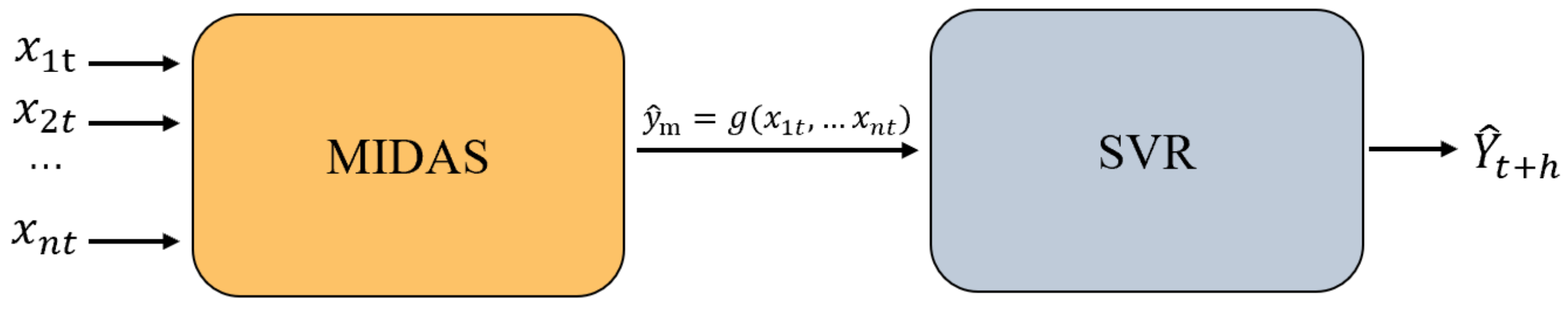
3.4. Prediction Results and Analysis Based on the MIDAS-SVR Model

This study seeks to predict future soybean price trends by means of a MIDAS-SVR forecasting model. Preprocessed data were used to predict prices within the R programming environment, with the detailed methodology outlined in Section 2. The model is initially trained with a training set to identify the optimal parameters for the MIDAS-SVR soybean price prediction model (refer to Table 4). Figure 3 illustrates the fitted values from the prediction model alongside the training set error metrics—the mean squared error (MSE) is 0.013, the mean absolute error (MAE) is 0.08, and the mean absolute percentage error (MAPE) is 1.36%. These results suggest that the model demonstrates high predictive accuracy.

Table 4. Parameter Settings of the MIDAS-SVR Model.

Parameter Name	Parameter Value	Parameter Name	Parameter Value
${\beta }_0$	1.711	$h$	1
${\beta }_1$	1.035	$m_1$	1
${\beta }_2$	$3.612\times {10}^{-2}$	$m_2$	1
${\beta }_3$	$-7.210\times {10}^{-2}$	$m_3$	1
${\beta }_4$	$2.147\times {10}^{-2}$	$m_4$	20
${\beta }_5$	$-5.653\times {10}^{-5}$	$m_5$	30
C	200	$ϵ$	0.1
$K\left(x_i,x_j\right)$	radial (RBF)	${\displaystyle \frac{1}{2{\sigma }^2}}$	0.01

Figure 3. Training Fitting Curve for MIDAS-SVR Soybean Price Prediction Model.

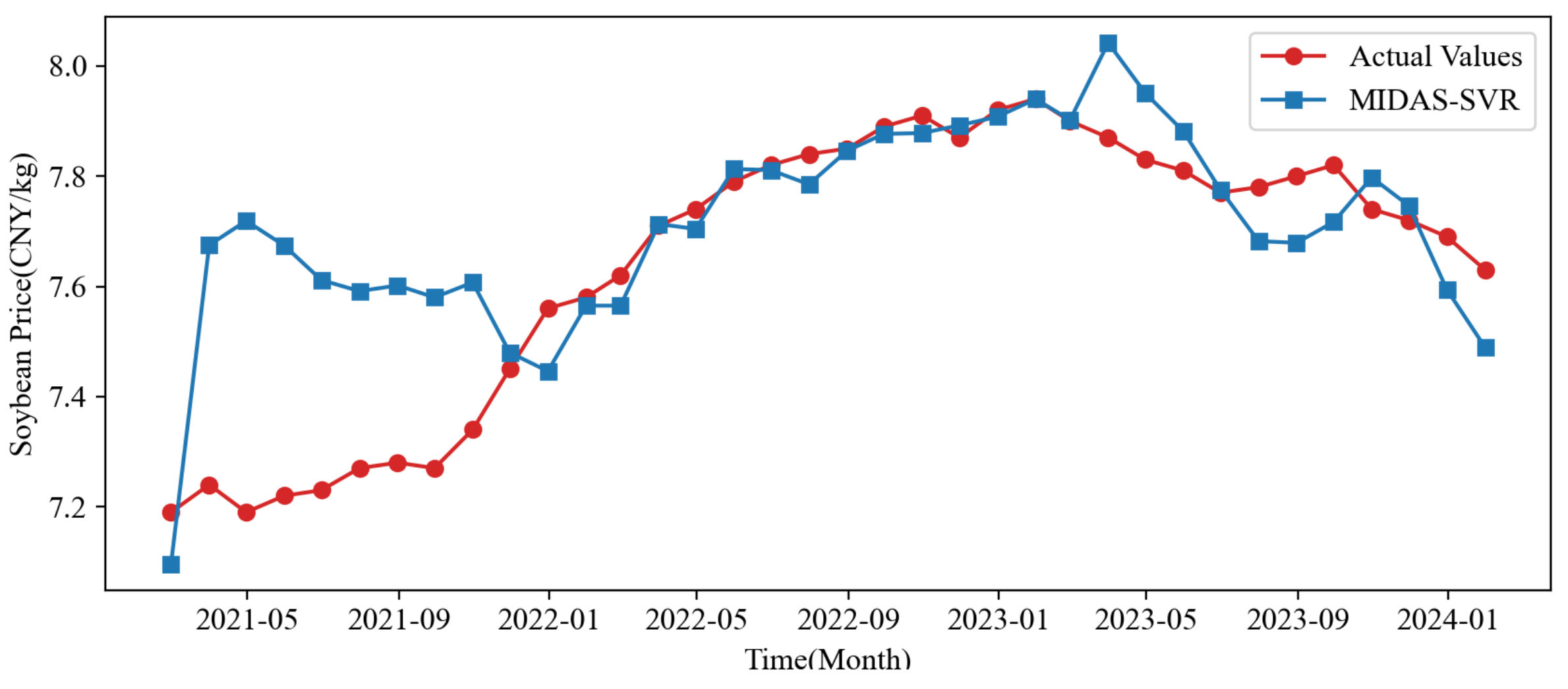
The variables for corn price, consumer price index, El Niño index, exchange rate, and Baidu soybean price index are arranged in ascending order. The notation represents the coefficient for the corn price variable while indicating the multiplicative relationship between the duration of the corn price cycle and that of the soybean price cycle, among other relationships. The MIDAS-SVR model was employed to predict soybean prices for the test sample covering February 2021 to January 2024, with the results presented in Table 5 and Figure 4. The prediction accuracy presented in Table 5 exhibits an initial trend of gradual improvement, followed by a plateau. The inaccuracy encountered in 2021 is likely associated with the ongoing effects of the COVID-19 pandemic. In early 2021, the volatility of soybean market prices escalated significantly due to supply chain disruptions, demand variations, and policy changes instigated by the pandemic, resulting in the suboptimal performance of the model during initial forecasts. After that, the uncertainty impact of the pandemic on the market decreased, and the accuracy of the model improved. Beginning in November 2021, there was a marked reduction in the model’s prediction error, with the relative error stabilizing at approximately 1%. This suggests that the model was better at capturing price trends during the later phases of the epidemic.

Table 5. Prediction Results and Error Analysis of the MIDAS-SVR Model on the Test Set.

Time	Actual Values	Predicted Values	ARE(%)	Time	Actual Values	Predicted Values	ARE(%)
February 2021	7.19	7.10	1.31	August 2022	7.85	7.85	0.05
March 2021	7.24	7.67	6.01	September 2022	7.89	7.88	0.17
April 2021	7.19	7.72	7.36	October 2022	7.91	7.88	0.40
May 2021	7.22	7.67	6.29	November 2022	7.87	7.89	0.28
June 2021	7.23	7.61	5.28	December 2022	7.92	7.91	0.15
July 2021	7.27	7.59	4.42	January 2023	7.94	7.94	0.00
August 2021	7.28	7.60	4.42	February 2023	7.90	7.90	0.03
September 2021	7.27	7.58	4.26	March 2023	7.87	8.04	2.18
October 2021	7.34	7.61	3.64	April 2023	7.83	7.95	1.54
November 2021	7.45	7.48	0.40	May 2023	7.81	7.88	0.91
December 2021	7.56	7.45	1.51	June 2023	7.77	7.78	0.07
January 2022	7.58	7.57	0.20	July 2023	7.78	7.68	1.26
February 2022	7.62	7.56	0.72	August 2023	7.80	7.68	1.55
March 2022	7.71	7.71	0.04	September 2023	7.82	7.72	1.32
April 2022	7.74	7.70	0.46	October 2023	7.74	7.80	0.74
May 2022	7.79	7.81	0.29	November 2023	7.72	7.75	0.34
June 2022	7.82	7.81	0.12	December 2023	7.69	7.59	1.25
July 2022	7.84	7.79	0.70	January 2024	7.63	7.49	1.84

Figure 4. Prediction Results of the MIDAS-SVR Model for Soybean Prices (Test Set).

3.5. Comparative Analysis

This study aims to rigorously evaluate the performance of the MIDAS-SVR model in forecasting soybean prices, particularly its capacity to analyze the intricate relationship between high-frequency factors and soybean prices. The MIDAS-SVR model is compared with five alternative models—a mixed-frequency data sampling (MIDAS) model, a traditional support vector regression (SVR) model using single-frequency data inputs (Baidu Index for Soybean Prices and average exchange rate), and a multilayer perceptron (MIDAS-MLP) model based on mixed-frequency data. The SVR model exclusively uses low-frequency data, specifically the monthly averages of the Baidu index and exchange rate variables. The MIDAS-MLP model parallels the MIDAS-SVR model by using predicted values from the MIDAS model as inputs for the MLP model; this is capable of directly processing mixed-frequency data, including high-frequency Baidu index and low-frequency economic indicators. We also compared the MIDAS-SVR model against standard time series models (auto-ARIMA and ETS). Figure 5 displays the fitted values for each model, showing how the six fitting curves align with trends observed in the actual sample curves.

Figure 5. Training Fitting Curves for the Four Prediction Models.

Figure 5 illustrates that the MIDAS model is less suitable for capturing soybean price trends than the other five models. In early 2016, mid-2017, and throughout 2019 and 2020, the fitted values of the MIDAS model exhibited significant deviations. The MIDAS-SVR and SVR models demonstrated a superior fit during that time period. Among the compared models, auto-ARIMA and ETS exhibit the highest fitting accuracy.

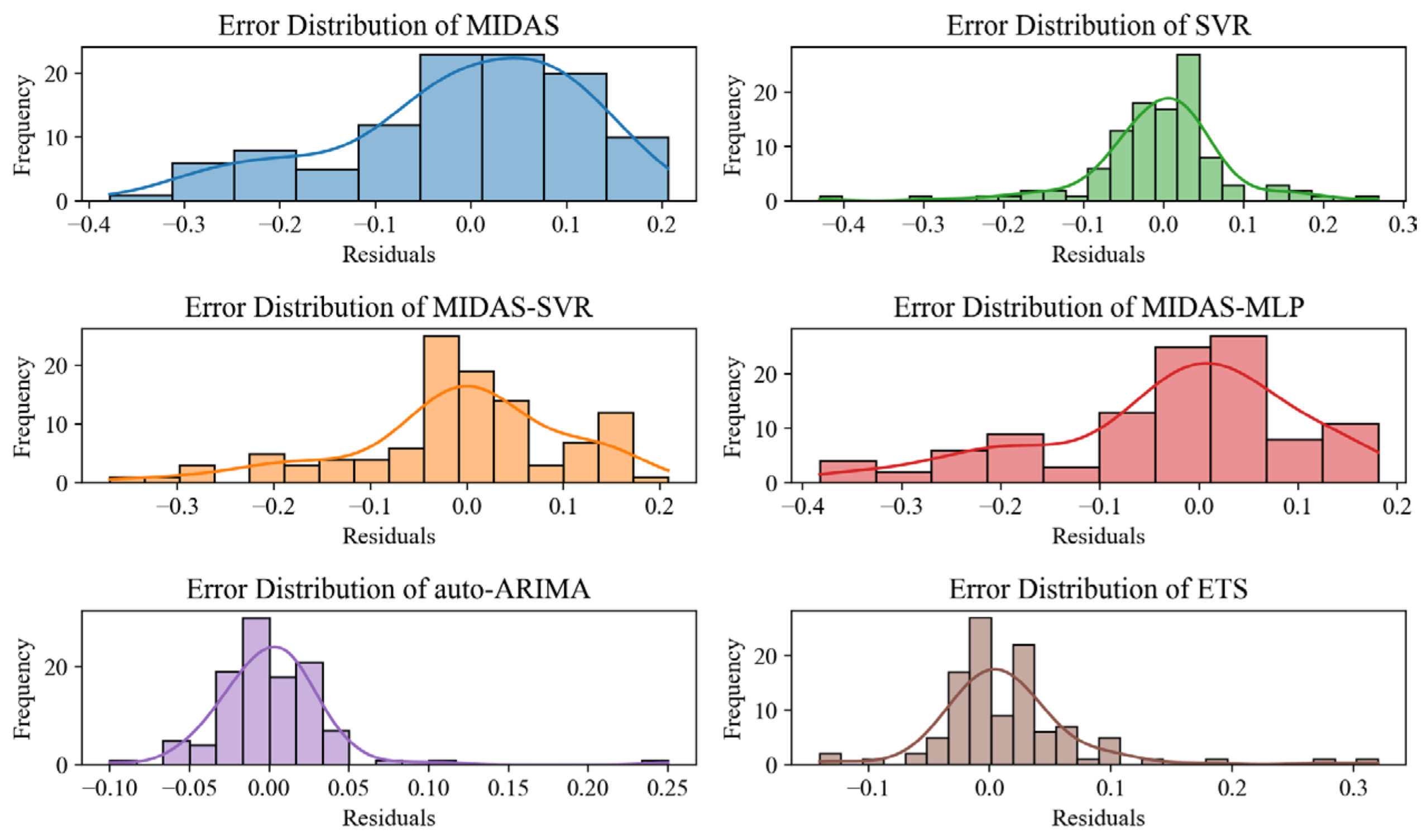
Figure 6 and Figure 7 present the residual histograms and residual boxplots for the six models, respectively. Figure 6 illustrates that the residuals of both the MIDAS model and the MIDAS-MLP model exhibit a distinctly left-skewed distribution, suggesting reduced stability. Figure 7 illustrates that the error means for each model approach zero, suggesting reduced bias within the training set. Additional analysis of the error distributions indicates that the auto-ARIMA and ETS models exhibit more concentrated error distributions with reduced fluctuation ranges, demonstrating better predictive stability. The error distributions of the MIDAS model and the MIDAS-MLP model exhibit greater dispersion, suggesting a higher level of uncertainty in their prediction outcomes.

Figure 6. Residual Analysis of the Four Models on the Training Set.

Figure 7. Boxplots of Residuals from the Six Models.

This study evaluated the forecasting performance of the MIDAS-SVR model by predicting soybean prices from February 2021 to January 2024 (test sample) using six different models. The results are presented in Table 6 and Figure 8.

Table 6. Prediction Errors of the Different Models (Test Set, February 2021–January 2024).

Model	MAPE	MAE	MSE
MIDAS	4.16%	0.32	0.13
SVR	2.36%	0.18	0.05
MIDAS-SVR	1.71%	0.13	0.04
MIDAS-MLP	2.02%	0.15	0.04
ETS	6.90%	0.53	0.50
Auto-ARIMA	14.41%	1.12	1.74

Figure 8. Prediction Results of the Six Models (Test Set).

The empirical results demonstrate significant performance limitations in traditional time series models, with ETS achieving 6.90% MAPE (MAE 0.50 and MSE 0.53) and auto-ARIMA performing substantially worse at 14.41% MAPE (MAE 1.74 and MSE 1.12) in out-of-sample testing. These limitations stem from fundamental structural constraints—while their linearity and stationarity assumptions provide protection against overfitting, they inherently restrict the models’ ability to capture complex nonlinear patterns. In contrast, our MIDAS-SVR framework achieves superior predictive accuracy (1.71% MAPE, MAE 0.04, and MSE 0.13), demonstrating reductions of 75.2%, 92.0%, and 75.5%, respectively, compared to ETS on these metrics. This performance advantage, extending to 88.1%, 97.7%, and 88.4% improvements over auto-ARIMA, validates that machine learning-enhanced mixed-frequency modeling can simultaneously achieve greater accuracy while maintaining robustness against overfitting.

Furthermore, comparative analysis reveals that MIDAS-SVR outperforms three alternative hybrid approaches—conventional MIDAS (4.16% MAPE), standard SVR (2.36% MAPE), and MIDAS-MLP (2.02% MAPE)—demonstrating the unique advantages of our proposed architecture in handling mixed-frequency data while avoiding overfitting.

3.6. Robustness Tests

Predictive robustness evaluates the stability and reliability of a predictive model’s outputs under varying conditions or environmental changes. This analysis seeks to confirm that the model consistently delivers accurate and reliable predictions in real-world applications, while also maintaining robust performance when confronted with data fluctuations, outliers, or unrealistic model assumptions. The paper employs two methods to assess the robustness of the model—a reduced training period (excluding the 2012 data) and an increased number of independent variables.

The MIDAS-SVR model was retrained by shortening the training set period (January 2013–January 2021), after which its predictive performance was assessed. Table 7 indicates that the set error, measured by MAPE, is 2.15%. In addition, the mean absolute error (MAE) exhibits an increase of 0.03 units, while the mean square error (MSE) shows a relative rise of 0.01 units. This suggests that a reduction in the training set data results in inadequate historical information being captured by the model, potentially diminishing its capacity for generalization. The error remains within an acceptable range.

Table 7. Robustness Test.

Plan	MAPE	MAE	MSE
Original MIDAS-SVR model	1.71%	0.13	0.04
Incorporating soybean meal price variables	1.72%	0.13	0.04
Reducing training time (January 2013–January 2021)	2.15%	0.16	0.05

This paper introduces soybean meal price as an explanatory variable to address potential omitted variable bias in the existing literature on factors influencing soybean prices. Upon incorporating the soybean meal price variable, the MIDAS-SVR model was re-evaluated, revealing that the mean relative error (MAPE) of the test set increased by a mere 0.01% (refer to Table 7). This suggests that the inclusion of explanatory variables slightly decreases the fitting accuracy on the training set while leaving prediction accuracy largely unaffected. The model presented in this paper successfully passed the robustness test, indicating that the research conclusions are very reliable.

4. Results and Discussion

Soybean prices are influenced by a variety of factors, including both macroeconomic data, which is typically reported on a quarterly basis, and low-frequency data, which is often available on a monthly basis. This paper employs a mixed-frequency data sampling (MIDAS) model to integrate daily data, such as weather and investor sentiment, with varying frequency sample data, all within a unified prediction framework. Our approach extends the work of Wang et al. (2023) by incorporating machine learning techniques to address known nonlinearity challenges in standard MIDAS applications [11]. Given the complexity and nonlinear nature of soybean price fluctuations, this study leverages the strengths of machine learning in handling intricate data. By fully exploring the nonlinear and discontinuous aspects of the data, the research combines machine learning with a mixed-frequency data sampling model to develop a mixed-frequency support vector regression (MIDAS-SVR) prediction model for soybean prices. Empirical research on soybean price data in China from January 2012 to January 2024 indicates that the MIDAS-SVR model demonstrates optimal predictive performance and improved stability, leading to the following key conclusions:

• There are four key dimensions that influence soybean prices: macroeconomic factors, supply and demand, weather, and public sentiment. Notably, the Consumer Price Index (CPI), corn prices, the El Niño Index, exchange rates, and the Baidu Index exhibit a significant correlation with fluctuations in soybean prices (p-values < 0.05). These findings align with Ferreira et al.’s (2022) demonstration of weather impacts on soybean markets [35].
• The MIDAS-SVR model improves prediction accuracy by using the information contained in high-frequency data, thus improving on traditional methods that merely simplify high-frequency data to single-frequency data through direct averaging.
• The MIDAS-SVR model demonstrates superior prediction accuracy and stability compared to other models, making it very suitable for capturing soybean price trends. The results obtained in this paper validate the MIDAS-SVR prediction model and offer new methodological support for soybean price prediction, opening up a wide range of theoretical and practical applications.

It should be noted that the current study has two main limitations: The model validation was conducted on a single commodity time series, and its generalizability to other agricultural markets requires further investigation. China-focused data may require calibration for global markets. Future research will expand the validation to multiple commodity markets and explore optimization techniques for practical implementation.