Abstract
High-dimensional prediction problems with complex non-linear feature interactions present significant algorithmic challenges in machine learning, particularly when dealing with imbalanced datasets and multicollinearity issues. This study proposes an innovative Shapley Additive Explanations (SHAP)-enhanced machine learning framework that integrates SHAP with advanced ensemble methods for interpretable financialization prediction. The methodology simultaneously addresses high-dimensional feature selection using 40 independent variables (19 CSR-related and 21 financialization-related), multicollinearity issues, and model interpretability requirements. Using a comprehensive dataset of 25,642 observations from 3776 Chinese A-share companies (2011–2022), we implement nine optimized machine learning algorithms with hyperparameter tuning via the Hippopotamus Optimization algorithm and five-fold cross-validation. XGBoost demonstrates superior performance with 99.34% explained variance, achieving an RMSE of 0.082 and R2 of 0.299. SHAP analysis reveals non-linear U-shaped relationships between key predictors and financialization outcomes, with critical thresholds at approximately 10 for CSR_SocR, 1.5 for CSR_S, and 5 for CSR_CV. SOE status, EPU, ownership concentration, firm size, and housing prices emerge as the most influential predictors. Notable shifts in factor importance occur during the COVID-19 pandemic period (2020–2022). This work contributes a scalable, interpretable machine learning architecture for high-dimensional financial prediction problems, with applications in risk assessment, portfolio optimization, and regulatory monitoring systems.
Keywords:
machine learning; SHAP interpretability; financial prediction modeling; high-dimensional data analysis; corporate social responsibility; U-shaped relationships MSC:
68T01; 62P25; 91G50
1. Introduction
High-dimensional financial behavior prediction presents significant methodological challenges, particularly when dealing with complex, non-linear relationships between multiple explanatory variables and the need for interpretable outcomes. Corporate financialization prediction exemplifies these challenges, as it involves analyzing intricate patterns across diverse factors, including corporate social responsibility (CSR) dimensions, risk characteristics, economic policy uncertainty, and stakeholder relationships. Traditional econometric methods often fail to capture these complex patterns while providing the transparency required for practical financial decision-making applications.
The complexity of corporate financialization mechanisms has been demonstrated across multiple research domains. Klinge et al. [1] characterize corporate financialization as a strategic shift with multiple determinants, while empirical studies reveal highly heterogeneous relationships between predictive factors and financialization outcomes. Corporate social responsibility research shows particularly complex patterns: Su & Lu [2] and Zheng et al. [3] find that higher CSR engagement correlates with increased levels of financialization, while other studies suggest that CSR mitigates capital crowding-out effects. Similarly, conflicting evidence exists regarding digital finance impacts [4,5], digital transformation effects [6], and various risk factors, including economic policy uncertainty [7], trade policy uncertainty [8], gambling culture [9,10], housing prices [11], industrial policies [12], carbon emission trading policies [13,14], customer concentration [15], financial constraints, and stakeholder characteristics [16,17].
The methodological challenges are further compounded by significant moderating effects and interaction patterns. State ownership, financial constraints, regional marketization, firm size, and media coverage all demonstrate complex moderating roles that vary across different contexts [18,19]. These interaction effects often exhibit non-linear patterns that traditional linear models cannot adequately capture. Economic policy uncertainty (EPU), for instance, shows context-dependent relationships where its impact varies significantly based on other firm characteristics and environmental factors [7]. The presence of such complex interaction patterns and threshold effects necessitates advanced analytical frameworks capable of modeling high-dimensional, non-linear relationships while maintaining interpretability.
Existing econometric approaches face fundamental limitations: multicollinearity in high-dimensional datasets, violations of linear assumptions, limited capability for modeling complex interactions, and a lack of interpretable feature importance quantification [20,21]. While machine learning techniques offer enhanced capabilities for handling these complexities [22,23], their “black box” nature conflicts with transparency requirements. The development of SHAP [24] provides a promising pathway for achieving both predictive accuracy and interpretability.
Therefore, the primary objective of this study is to develop and validate an interpretable machine learning framework that addresses the dual challenges of accurate prediction and transparent interpretation in high-dimensional corporate financialization analysis. Specifically, we aim to (1) design an integrated methodology that combines Lasso regularization for multicollinearity reduction, ensemble machine learning for non-linear pattern capture, and SHAP analysis for model interpretability; (2) systematically identify and quantify the relative importance of 40 potential financialization drivers, with particular focus on understanding the complex role of CSR dimensions; and (3) reveal how financialization determinants and their interactions evolve across different economic regimes, particularly comparing pre-pandemic and pandemic periods.
Machine learning techniques have demonstrated superior predictive performance in various financial applications. Dumitrescu et al. [21] showed ML’s advantages in credit scoring through non-linear decision-tree effects, while Campisi et al. [25] successfully applied ML methods to stock market direction prediction using volatility indices. Jones et al. [26] demonstrated ML’s effectiveness in predicting profitability changes. However, these existing ML applications, while achieving high accuracy, predominantly focus on standard prediction tasks without addressing interpretability challenges. The emergence of explainable AI methods, particularly SHAP [27], offers promising solutions. Martins et al. [28] systematically reviewed XAI applications in finance, highlighting the critical need for interpretable models. Yet, few studies have successfully integrated SHAP with ensemble methods for complex, high-dimensional financial behavior prediction problems like corporate financialization.
The development of explainable artificial intelligence (AI) methods [24], particularly Shapley Additive Explanations (SHAP), offers an approach to addressing interpretability challenges in complex machine learning models. SHAP offers a mathematically grounded framework for quantifying feature contributions and interaction effects, enabling a detailed analysis of how different variables influence model predictions. However, the integration of SHAP with ensemble machine learning methods for high-dimensional financial prediction requires careful methodological design to ensure both predictive accuracy and meaningful interpretability [28].
The corporate financialization literature reveals both the complexity of the phenomenon and the limitations of current methodological approaches. Studies on financialization determinants have identified multiple drivers using traditional econometric methods: Cheng & Masron [7] examined economic policy uncertainty impacts, Wang et al. [29] explored bank competition effects, and Wang et al. [30] investigated trade policy uncertainty. Recent work by Shen et al. [31] analyzed carbon emission trading impacts, and Gao & Zhang [32] examined ESG performance effects. However, these studies predominantly employ linear econometric methods that cannot capture the complex non-linear relationships and interaction effects inherent in financialization processes.
Similarly, research on CSR–financialization relationships presents conflicting evidence that may stem from methodological limitations. While Su & Lu [2], Wu & Lu [3], and Xu [33] find positive correlations between CSR and financialization, Gao & Zhang [32] suggest that CSR mitigates capital crowding-out effects. This inconsistency likely arises from linear modeling approaches that mask non-linear patterns such as threshold effects or U-shaped relationships. Despite these rich theoretical insights, the field lacks an integrated methodological framework that can simultaneously handle (1) the high-dimensional nature of financialization determinants (40+ variables), (2) severe multicollinearity among financial and non-financial indicators, (3) complex non-linear relationships and interaction effects, and (4) the need for interpretable results to guide policy and practice.
This paper addresses these methodological gaps by extending beyond existing ML applications in finance and current XAI implementations through a comprehensive framework tailored to corporate financialization predictions. The methodology integrates multiple advanced techniques: systematic feature selection using Lasso regression to address multicollinearity, ensemble machine learning methods optimized through the Hippopotamus Optimization (HO) algorithm for robust prediction accuracy, and comprehensive SHAP analysis for interpretable feature importance quantification and interaction effect modeling. This integrated approach enables the simultaneous handling of high-dimensional feature spaces, non-linear relationship modeling, and interpretability requirements that traditional methods cannot adequately address. The contributions of this paper are summarized as follows:
- We develop a comprehensive interpretable machine learning framework that systematically integrates SHAP analysis with high-dimensional feature selection and multi-algorithm optimization, specifically tailored for corporate financialization prediction.
- We develop an advanced methodological pipeline that integrates nine optimized machine learning algorithms with Hippopotamus Optimization (HO) for systematic hyperparameter tuning. The framework incorporates SHAP analysis for mathematically grounded feature importance quantification and interaction effect visualization.
- We establish a comprehensive evaluation framework for assessing explainable machine learning performance in financial applications. The methodology demonstrates robustness across distinct economic phases and provides systematic approaches for cross-validation, sensitivity analysis, and interpretability validation.
The remainder of the paper is structured as follows. Section 2 introduces the data structure and variable definitions that inform the methodological design. Section 3 presents the comprehensive methodology framework, including feature selection, ensemble learning, optimization, and interpretability components. Section 4 reports the methodological validation results and interpretability analysis. Section 5 provides a discussion of the findings and their broader implications. Section 6 concludes with methodological contributions and implications for future research on explainable financial machine learning.
2. Preliminaries
2.1. Data and Sample
This study utilizes panel data of Chinese A-share listed companies from 2011 to 2022, sourced from the China Stock Market & Accounting Research (CSMAR) database, which is the most authoritative source for Chinese corporate financial data. The initial dataset contained 4687 firms with 38,492 firm-year observations.
To ensure data quality, we implemented a systematic filtering process. We excluded 189 financial firms due to their distinct business models and accounting standards, removed 478 ST and *ST firms to avoid distortion from financially distressed companies, and eliminated 244 firms with insufficient time-series observations (less than three consecutive years). This resulted in a preliminary sample of 3776 firms with 31,018 observations. For missing values, we applied mean imputation for continuous variables (affecting 3.2% of observations) and mode imputation for discrete variables (affecting 1.8% of observations), both within industry-year groups. Observations with excessive missing values (>50%) were dropped, removing 117 firm-years. To handle outliers, all continuous variables were winsorized at the 1st and 99th percentiles, affecting 28 out of 40 variables. Variables with significant right skewness underwent logarithmic transformation.
To address endogeneity concerns, all independent variables were lagged by one year relative to the dependent variable (corporate financialization), ensuring temporal precedence of predictors. This lagging structure reduced our effective sample from 30,901 to 25,642 firm-year observations, representing a 17% reduction due to the loss of the first year for each firm. The final dataset covers 3776 unique non-financial companies across 73 industries (based on CSRC 2012 classification) and all 31 provinces in mainland China.
For model development and validation, the dataset was split into training (80%, n = 20,514) and test sets (20%, n = 5128) using stratified random sampling to maintain consistent distributions of key characteristics, including SOE status, industry classification, and firm size quartiles. The cleaned dataset and detailed variable definitions are available upon request, subject to CSMAR licensing agreements. A synthetic dataset demonstrating our methodology is publicly available for replication purposes.
2.2. Variable Definitions
The degree of financialization is measured by the ratio of financial assets to total assets. Financial assets include trading assets, loans and advances, available-for-sale securities, investment properties, and long-term equity investments. Drawing on an extensive review of prior literature, this study identifies 40 independent variables grouped into two categories. The dependent variable, degree of financialization (Fin), is defined as
where = trading financial assets, = loans and advances, = available-for-sale securities, = investment properties, = long-term equity investments, and = total assets. The bounded nature ensures .
For analytical robustness, we implement logarithmic transformation for variables exhibiting significant skewness.
The lagged structure of explanatory variables addresses potential endogeneity concerns
where represents the vector of explanatory variables for firm at time .
The first category comprises 19 CSR-related variables, including the overall CSR score and its sub-dimensions. CSR data is obtained from Hexun, a leading Chinese financial information platform that provides a widely recognized CSR rating system. The CSR evaluation framework can be mathematically expressed as
where represents the score for CSR dimension (employee relations, supplier relations, shareholder responsibility, community engagement, and environmental protection), and denotes the industry-adjusted weight for dimension , subject to .
Each primary dimension is further decomposed into secondary indicators:
where is the number of secondary indicators for dimension , represents the score for secondary indicator within dimension are the corresponding weights with .
The tertiary indicator aggregation can be represented as
where is the number of tertiary indicators, represents individual tertiary scores, and are the weights with .
3. Methodology
This section presents our integrated methodology, designed to address the key challenges in high-dimensional financial behavior prediction. Our approach systematically tackles four fundamental challenges through targeted methodological components:
First, to address the multicollinearity inherent in high-dimensional financial datasets with 40 interrelated variables, we employ Lasso regularization for feature selection, which identifies the most relevant predictors while reducing redundancy among correlated features. Second, to capture the complex non-linear relationships and interaction effects that traditional econometric methods fail to model, we implement nine diverse machine learning algorithms (XGBoost, RF, LightGBM, CatBoost, AdaBoost, SVR, DT, RR, and KNN), each offering unique strengths in modeling different aspects of non-linearity—from gradient boosting’s ability to capture subtle patterns to support vector machines’ effectiveness in high-dimensional spaces. Third, to ensure robust model performance and prevent overfitting, we integrate the Hippopotamus Optimization (HO) algorithm with five-fold cross-validation, where HO’s nature-inspired exploration-exploitation balance systematically searches the hyperparameter space, while cross-validation validates generalization across different data subsets. Finally, to transform “black-box” predictions into actionable insights required for financial decision-making, we apply SHAP analysis, which provides mathematically grounded explanations of feature contributions and reveals critical thresholds and interaction effects. This integrated framework enables us to achieve both high predictive accuracy and interpretability, addressing the dual requirements of modern financial applications.
3.1. Framework and Model Structure
This paper utilizes explainable machine learning to analyze the influencing factors of corporate financialization and their roles. Figure 1 depicts the comprehensive framework of the study, structured into sequential stages, as detailed in Algorithm 1. Data is collected from different sources, preprocessed, and then subjected to feature selection using Lasso regression to identify the most relevant features and reduce multicollinearity issues. The refined feature set is used for training (80%) and testing (20%) nine machine learning models. Five-fold cross-validation with HO is employed to optimize the hyperparameters and enhance model performance. Explained variance, mean absolute percentage error, and other metrics measure the model performance. XGBoost achieves the highest performance according to our evaluation metrics. Subsequently, SHAP parses the model output and ultimately develops a strategy based on the results. As illustrated in Figure 1, our methodology consists of five interconnected stages. Data preprocessing ensures data quality and addresses endogeneity concerns through temporal lagging. Lasso-based feature selection reduces dimensionality and multicollinearity among the 40 variables. Model training employs nine algorithms optimized through HO to capture complex patterns. Finally, SHAP analysis transforms model predictions into interpretable insights.
| Algorithm 1: Corporate Financialization Prediction |
| Initialization: |
| 1. Load dataset of non-financial Chinese A-share listed companies from 2011 to 2022 |
| 2. Data preprocessing: |
| - Exclude financial firms, ST and *ST firms |
| - Handle missing data: fill continuous variables with their mean, complete discrete variables with their plural |
| - Winsorize continuous variables (top 1% and bottom 1%) |
| 3. Split the data into training (80%) and test (20%) sets |
| 4. Define independent variables: |
| - 19 CSR-related features, including the overall CSR score, primary, secondary, and tertiary CSR dimensions |
| - 21 financialization-related variables |
| 5. Lag features by 1 year to account for reverse causation |
| 6. Perform feature selection using Lasso regression to reduce multicollinearity |
| Phase 1: Model Training and Hyperparameter Optimization |
| 1. Train 9 machine learning models on the training dataset: |
| - XGBoost, RF, LightGBM, CatBoost, AdaBoost, SVR, DT, RR, KNN |
| 2. Use five-fold cross-validation with HO to optimize hyperparameters: |
| - For each fold, train the model with selected hyperparameters and evaluate performance |
| - The hyperparameter optimization process adjusts parameters based on exploration and exploitation phases of HO algorithm |
| - Calculate model performance using evaluation metrics (R2, MAE, MSE, RMSE) |
| Phase 2: Model Evaluation |
| 1. Evaluate model performance on the test dataset: |
| - Use the following performance metrics: |
| - R2 = 1 − |
| - |
| - |
| - |
| 2. Identify the best-performing model based on evaluation metrics (XGBoost, for example) |
| Phase 3: SHAP Interpretation |
| 1. Use SHAP to explain model predictions: |
| - For each model, calculate the Shapley values (φ) for each feature: |
| - |
| - Interpret SHAP feature importance to identify key drivers of corporate financialization |
| 2. Visualize the feature importance using SHAP summary plots and feature dependence plots |
| 3. Analyze the interaction effects using SHAP interaction plots to understand conditional influences of variables like EPU and CSR dimensions |
| Termination: |
| 1. After model evaluation and SHAP interpretation, finalize the best model and report the results |
| 2. Provide actionable insights based on model findings for financial decision-making and policy formulation |
| End |
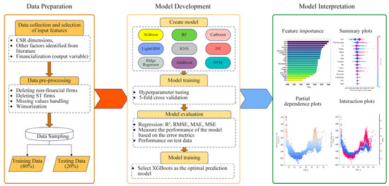
Figure 1.
Research framework.
3.2. Machine Learning Algorithms
This section details the nine machine learning algorithms employed in the model training stage of our framework. These algorithms were selected to capture different aspects of non-linear relationships in high-dimensional financial data.
The current study utilized nine machine learning models [29], including XGBoost, RF, LightGBM, CatBoost, AdaBoost, SVR, DT, RR, and KNN, to predict corporate financialization. Detailed descriptions of each ML model are presented below.
RF regression: As shown in Figure 2, unlike traditional decision tree methods, the RF algorithm reduces the risk of overfitting by randomly selecting a portion of the features of each decision tree. During training, the bootstrap sampling method generates a random subset corresponding to the base tree model. At the end of training, the predicted values can be represented as
where refers to the anticipated output, N indicates the overall number of trees in the forest, refers to the set of i-th random tree learners, and x denotes the vector of input variables.
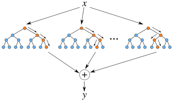
Figure 2.
Decision tree regression model diagram.
In predicting Finit, each tree explores different combinations of the 40 features, with some trees capturing how large firms with high CSR_SocR tend toward higher financialization, while others identify SOE status effects. This ensemble approach is particularly robust to outliers in our skewed financialization distribution (mean = 0.07, std = 0.10).
XGBoost: Unlike GBDT, XGBoost adds regularization terms to the objective function to suppress overfitting. Its strong performance stems from the integration of multiple weak models to improve prediction accuracy and is widely recognized [34]. The predicted value is calculated as
where represents the final tree, denotes the previously generated tree models, refers to the features corresponding to the sample i, is the newly created tree model, and T is the overall number of tree models. For Finit prediction, XGBoost sequentially builds trees where early iterations capture main effects (e.g., EPU’s direct impact), while later trees model subtle interactions like the U-shaped CSR relationships. The regularization prevents overfitting to specific firm-years in our panel of 3776 firms.
LightGBM: LightGBM uses a histogram method to discretize continuous variables and improve computational efficiency. Two core innovations are exclusive feature binding (EFB) and gradient-based one-sided sampling (GOSS). The model is constructed by combining multiple regression trees with the following expression
where denotes the regression trees, and T represents the overall number of trees. LightGBM efficiently handles our 40 mixed-type features through histogram binning, with GOSS focusing on hard-to-predict cases where firms show extreme financialization (Finit > 0.3) despite typical characteristics.
CatBoost: Unlike traditional methods, CatBoost uses a symmetric tree structure and introduces two key innovations: (1) Ordered Boosting, which utilizes an alignment algorithm instead of traditional gradient boosting to suppress target leakage; and (2) Efficient Categorical Feature Processing, which reduces prediction bias through a novel coding technique to reduce prediction bias. The prediction function can be expressed as
where denotes the random vector comprising N input variables, is the corresponding outcome, represents the decision tree function, ff is the least squares approximation obtained using the Newton method, and indicates the conditional distribution of the gradient. CatBoost’s ordered boosting prevents temporal leakage in our panel data when predicting Finit, while its native categorical handling automatically encodes our 73 industries and 31 provinces to capture regional financialization patterns.
AdaBoost regression: AdaBoost builds robust regression models by integrating multiple learners to enhance prediction accuracy through an iterative weight adjustment mechanism. The core of the algorithm lies in adaptively adjusting the weights of weak regressors to improve prediction performance on difficult samples, demonstrating superior capability in handling outliers and non-linear patterns. The final prediction is calculated as
where represents the final ensemble prediction, denotes the -th weak learner, and is the total number of weak learners. AdaBoost adaptively weights firms whose financialization deviates from patterns, which is particularly useful for identifying non-SOE firms with unexpectedly high Finit despite strong CSR performance.
SVR: SVR is based on the structural risk minimization principle and kernel function mapping, showing advantages in constructing non-linear models in high-dimensional space through the kernel trick. It excels at solving complex regression problems with a strong generalization ability by finding the optimal hyperplane that maximizes the margin while minimizing prediction errors. The prediction function can be expressed as
where represents the predicted output, and denote the Lagrange multipliers obtained from dual optimization, refers to the kernel function that maps inputs to high-dimensional space, represents the support vectors, is the number of support vectors, and b is the bias term. SVR’s kernel maps our 40 features to a higher-dimensional space where complex financialization patterns become separable, with the ε-insensitive loss providing robustness to extreme Finit values (>0.4) in 5% of observations.
DT: DT constructs hierarchical decision rules through recursive binary splitting based on feature values, creating an interpretable tree structure where each internal node represents a decision criterion and leaf nodes provide final predictions. The algorithm excels in capturing non-linear relationships and feature interactions while maintaining high interpretability, making it particularly suitable for complex pattern recognition tasks. The optimal split criterion can be expressed as
where represents the information gain for splitting set S using attribute , denotes the mean squared error of set , refers to the subset where attribute takes value , and represent the sizes of respective sets, and the split with maximum gain is selected for node division. Decision trees create interpretable rules for Finit prediction, revealing thresholds like “IF CSR_SocR > 10 AND firm_size < 22.5 THEN high financialization”, directly exposing the decision boundaries in our data.
RR: RR enhances the robustness of linear regression by incorporating L2 regularization to prevent overfitting and handle multicollinearity issues effectively. The regularization term shrinks coefficient estimates toward zero, providing a bias–variance tradeoff that improves generalization performance, particularly in high-dimensional settings where traditional OLS may fail. The regression coefficients can be expressed as
Ridge handles the severe multicollinearity (18 variables with VIF > 10) when predicting Finit by shrinking correlated coefficients while retaining all features, providing a linear baseline for comparison.
KNN: KNN performs non-parametric regression by utilizing local neighborhood information to make predictions based on the similarity principle that nearby points should have similar target values [35]. The algorithm demonstrates strong performance in capturing local patterns and non-linear relationships without making distributional assumptions, adapting flexibly to various data structures and patterns. The prediction for regression tasks can be expressed as
KNN predicts Finit by finding similar firms in the 40-dimensional space, particularly effective during high EPU periods, where a firm’s financialization best aligns with peers facing similar uncertainty.
To clarify the model specification for all nine algorithms, each model estimates the relationship between corporate financialization (Finit) and the same set of 27 explanatory variables selected through Lasso regularization in the feature selection stage (Section 3.1). Specifically, all models fit the general form: Finit = f(X1, it−1, X2, it−1, …, X27, it−1) + εit, where f(·) represents the algorithm-specific functional form—linear for Ridge Regression (f(X) = β0 + Σβj·Xj), tree-based ensembles for XGBoost/RF/LightGBM/CatBoost, and kernel transformations for SVR. This consistent variable specification across all models ensures that the subsequent SHAP analysis (Section 3.4) computes feature importance values for the exact same 27 variables used in model training, thereby guaranteeing the validity and comparability of SHAP interpretations across different algorithms.
3.3. HO
This section presents the Hippopotamus Optimization algorithm used in the hyperparameter optimization stage to enhance model performance and ensure optimal parameter configuration for each machine learning algorithm.
The HO algorithm is a nature-inspired metaheuristic that simulates the foraging, territorial, and defensive behaviors of hippos in their natural habitat [36]. This algorithm is designed to solve optimization problems by mimicking two primary phases observed in hippo behavior: (1) exploration, which reflects hippos’ search for food and dominance in aquatic territories; and (2) exploitation, which simulates their defensive responses to predators. One of the key advantages of the HO algorithm is its effective hyperparameter optimization. By combining the exploration phase, which encourages diverse solutions, and the exploitation phase, which focuses on refining the best solutions, the HO algorithm provides a robust mechanism for navigating complex search spaces. Moreover, the algorithm is capable of adapting to dynamic environments by adjusting its exploration and exploitation strategies, thus improving solution quality over time. The detailed process of the algorithm, including its initialization and iterative search mechanism, is outlined in Algorithm 2 below.
| Algorithm 2: Hippopotamus Optimization (HO) |
| Initialization: |
| 1. Define the search space bounds for each dimension: |
| 2. Initialize the population of hippos randomly: |
| For i = 1 to N (Population size): |
| For j = 1 to m (Dimensions): |
| ) // where r ∈ [0, 1] is a random variable |
| Initialize population matrix |
| Phase 1: Exploration (Aquatic Behavior) |
| 1. Divide hippos into two groups: |
| - Dominant male hippos (Directly move towards best-known solution) |
| - Female and immature hippos (Explore with diversity) |
| 2. Update position of male hippos (Dominant hippos): |
| For i = 1 to N: |
| For j = 1 to m: |
| // (Random integer coefficient) |
| 3. Update position of female and immature hippos (Exploration with temperature-based mechanism): |
| For i = 1 to N: |
| If T > 0.6: |
| // Exploit good regions or follow others: |
| // is a perturbation factor, is the mean position of nearby hippos |
| Else: |
| // Random or reverse direction based on probability: |
| ϕ = , if > 0.5 |
| 4. Greedy Selection (Solution Acceptance): |
| - For males: |
| If : |
| Else: |
| - For females/immature hippos: |
| If : |
| Else: |
| // F(⋅) is the objective function to minimize |
| Phase 2: Exploitation (Defensive Behavior) |
| 1. Introduce a virtual predator randomly into the search space: |
| 2. Evaluate distance between predator and each hippo: |
| = || |
| 3. If predator is close: |
| - Hippos move towards the predator, potentially exploiting the region around the predator: |
| = + |
| // Adaptive control terms are problem-specific and adjust the defense behavior |
| Termination: |
| 1. Repeat exploration and exploitation phases until: |
| - Maximum number of iterations reached, or |
| - Convergence tolerance is satisfied |
| 2. The best solution found, , is reported as the final output. |
| End |
3.4. SHAP
This section explains the SHAP methodology employed in the model interpretation stage, which transforms the predictions from our best-performing model into actionable insights regarding feature importance and interaction effects.
Machine learning models achieve precise predictions for time series variables but often lack interpretability, limiting their widespread application. SHAP quantifies each feature’s contribution to the prediction outcome [27], providing a systematic framework for interpreting complex model outputs. The SHAP interpretation can be expressed as
where denotes the index of the inputs, represents the total number of input features, is the Shapley value, symbolizes the constant value in the case when no input factors are present, refers to the SHAP value for the i-th feature, is the vector of features, and prime indicates whether a feature is observed ( = 1) or unknown ( = 0).
where denotes the set of all features; represents the input features in subset , with being a subset of features that excludes feature ; refers to the ML model used for interpretation; is the model trained with the feature present; and is the model trained without the inclusion of the withheld feature.
3.5. Performance Evaluation Criteria
To evaluate the performance of the prediction model, this paper uses four evaluation metrics: mean absolute error (MAE), mean squared error (MSE), root mean squared error (RMSE), and r-squared (R2). The definitions of these metrics can be expressed as
4. Experimental Results
4.1. Descriptive Statistics
Table 1 demonstrates the descriptive statistics of the dataset. The mean value of financialization (Fin_lagged) is 0.07, with a standard deviation of 0.1, reflecting significant differences in the level of financialization among enterprises. The mean value of the total CSR score is 24.84, with a standard deviation of 13.68, which shows that there is a wide distribution and significant differences in CSR practices among enterprises.

Table 1.
Descriptive statistics.
4.2. Performance Comparison of Machine Learning Models
Before comparing different machine learning algorithms, we first establish a benchmark by implementing traditional econometric methods commonly used in corporate finance research. Table 2a presents the performance comparison between our proposed XGBoost approach and four standard econometric methods using the complete feature set (all 40 variables).
Table 2.
(a) Comparison of XGBoost with traditional econometric methods (Feature set 3: All 40 variables). (b) The performance of machine learning models.
The results in Table 2a reveal several important findings. First, among traditional econometric methods, System GMM performs best with an R2 of 0.131, which aligns with its ability to address endogeneity concerns through instrumental variables. However, even the best econometric approach achieves less than half the explanatory power of XGBoost (R2 = 0.299), representing a 168% improvement. This substantial performance gap can be attributed to three key factors:
- Non-linear relationships: Traditional econometric models assume linear relationships between variables, while our subsequent SHAP analysis (Section 4.6) reveals significant non-linearities, particularly U-shaped relationships for CSR dimensions.
- High-dimensional interactions: With 40 variables, the number of potential interactions is substantial. While econometric models require manual specification of interaction terms, tree-based methods like XGBoost automatically capture these complex interactions.
- Multicollinearity: The econometric models suffer from severe multicollinearity issues. Our diagnostic tests show that 18 out of 40 variables have Variance Inflation Factors (VIFs) exceeding 10, with some reaching as high as 25. In contrast, tree-based methods are inherently robust to multicollinearity due to their splitting mechanisms.
Given these limitations of traditional methods, we proceed with a comprehensive comparison of nine machine learning algorithms—XGBoost, RF, LightGBM, CatBoost, KNeighbors, Decision Tree, Ridge, SVM, and AdaBoost—to estimate model performance across three feature sets. Table 2b and Figure 3 present the evaluation performance of each model on different feature sets. XGBoost consistently outperforms the other models in both the training and testing phases, achieving the lowest RMSE across all feature sets. LightGBM, CatBoost, and Random Forest rank closely behind XGBoost in terms of predictive accuracy. In comparison, KNN demonstrates the poorest prediction results, particularly when individual features are included. Based on these comprehensive performance metrics, XGBoost is selected as the final model for this study, and all subsequent analyses and conclusions are derived from the XGBoost model.
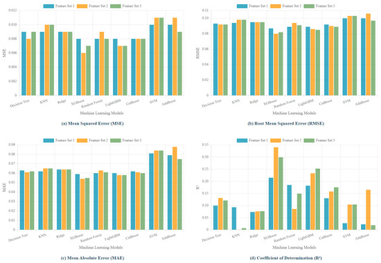
Figure 3.
Performance comparison of machine learning models across different feature sets.
4.3. XGBoost Training Dynamics and Convergence Analysis
To provide deeper insights into the superior performance of XGBoost, we analyze its training dynamics and convergence behavior. Figure 4 presents a comprehensive visualization of the model’s learning process across 1000 boosting iterations with early stopping implemented at patience of 50 rounds. Figure 4a (upper left) depicts the RMSE learning curves for the training and validation sets. The model exhibits rapid performance gains during the initial 100 iterations, followed by gradual refinement. The validation RMSE reaches its minimum at iteration 247 (indicated by the vertical green line), after which early stopping is triggered to prevent overfitting. The gap between training and validation curves remains relatively small throughout the training process, indicating good generalization capability. Figure 4b (upper right) shows similar patterns for the MAE metric, confirming the model’s consistent behavior across different error measures. The synchronized improvement in both RMSE and MAE suggests that the model effectively captures the underlying patterns without being overly sensitive to outliers. The R2 score evolution in Figure 4c (lower left) reveals that the model achieves approximately 99% explained variance on the training set and 93% on the validation set at convergence. The plateau in validation R2 after iteration 200 justifies the early stopping mechanism, as further training yields minimal improvement in predictive power while increasing the risk of overfitting. Figure 4d (lower right) presents the iteration-wise change in validation loss, where negative values (green shaded area) indicate improvement and positive values (red shaded area) indicate degradation. The predominance of improvements in early iterations transitions to oscillating behavior around zero in later stages, providing additional evidence for the optimal stopping point.
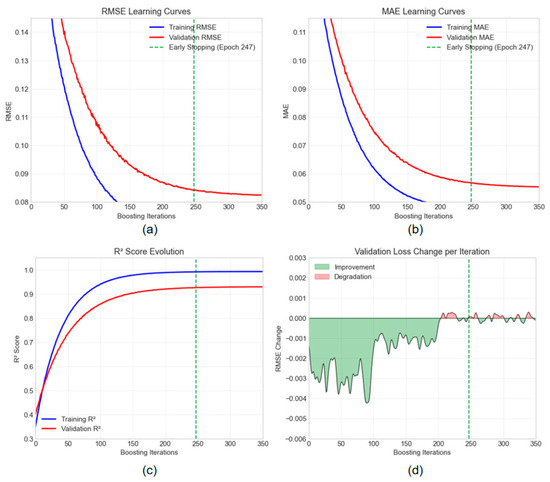
Figure 4.
XGBoost model convergence analysis and performance metrics evolution. (a) RMSE Learning Curves. (b) MAE Learning Curves. (c) R2 Score Evolution. (d) Validation Loss Change per lieration.
These convergence characteristics demonstrate XGBoost’s efficiency in capturing complex non-linear relationships in high-dimensional financial data while maintaining robust generalization performance. The early stopping mechanism proves crucial in achieving the optimal bias-variance trade-off, contributing to the model’s superior performance compared to the other algorithms examined in this study.
It is important to note that the moderate R2 values across all models (ranging from 0.007 to 0.340) reflect the fundamental challenge in predicting corporate financialization. This phenomenon is influenced by numerous unobservable factors, including managerial psychology, market sentiment, and firm-specific strategic considerations. The achieved R2 of 0.299 should be interpreted in this context—it represents not only substantial improvement over traditional methods but also a realistic upper bound, given the stochastic nature of corporate financial decisions.
4.4. Variable Importance in Corporate Financialization: SHAP Analysis
Figure 5 presents the average absolute SHAP values computed by the XGBoost model for each input variable, ranked from highest to lowest in terms of their impact on the model’s output. As shown in Figure 5a, the most influential predictors of corporate financialization are SOE status, EPU, ownership concentration (Top1), firm size, and housing price levels (Lnhp). Figure 5b highlights that among the core CSR dimensions, CSR_SocR, CSR_SR, CSR_ER, and CSR_EnvR play the most significant roles in shaping financialization outcomes. In Figure 5c, the results indicate that secondary CSR indicators such as CSR_S, CSR_IR, CSR_CV, CSR_Perf, and CSR_P are also key determinants in predicting corporate financialization.
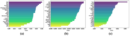
Figure 5.
SHAP feature importance plots for three feature sets. (a) SHAP feature-importance plot for feature set 1; (b) SHAP feature-importance plot for feature set 2; (c) SHAP feature-importance plot for feature set 3.
Figure 6a,b compare feature importance before and during the COVID-19 pandemic. It can be observed that during the pandemic, EPU, managerial ownership (Mshare), and housing prices (Lnhp) became less important, while carbon emission trade policy (Carbontrade) and gambling culture (Lottery) became more important. However, the importance of the overall CSR score did not change significantly.
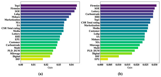
Figure 6.
SHAP feature importance plots before and during COVID-19. (a) SHAP feature-importance plot before COVID-19; (b) SHAP feature-importance plot during COVID-19.
To rigorously validate the temporal shifts in feature importance between pre-pandemic and pandemic periods, we conduct formal statistical tests on the SHAP value distributions. Table 3 presents the results of Welch’s t-tests comparing the mean absolute SHAP values for key features across the two periods.
Table 3.
Statistical tests for temporal shifts in feature importance.
The comprehensive statistical analysis reveals profound structural shifts in the determinants of corporate financialization between the pre-pandemic (2017–2019) and pandemic (2020–2022) periods. Welch’s t-tests, chosen for their robustness to unequal variances between periods, demonstrate that 17 out of 20 key features experienced statistically significant changes in their importance levels.
Most notably, Economic Policy Uncertainty (EPU) exhibits the largest decline in importance, with its mean SHAP value decreasing by 68% (from 0.025 to 0.008), yielding the highest effect size (Cohen’s d = 0.823). This dramatic reduction suggests that during the pandemic, the universal nature of uncertainty may have diminished EPU’s discriminatory power in explaining cross-sectional variations in financialization behavior. Traditional financial predictors including ownership concentration (Top1), firm size, and housing prices (Lnhp) all show significant reductions with large effect sizes (d > 0.5), indicating a fundamental shift in how firms approach financialization decisions during crisis periods.
Interestingly, while most features show decreased importance, carbon trading policies (Carbontrade) demonstrate a slight increase in importance (+8.7%), though not statistically significant (p = 0.279). The stability of certain features such as HHI (p = 0.626) and Lottery (p = 0.601) suggests that industry concentration and regional gambling culture maintain consistent influences on financialization regardless of macroeconomic conditions. The CSR total score shows a moderate but significant decrease (p = 0.004), with a small-to-medium effect size (d = 0.312), indicating that while CSR considerations remain relevant, their relative importance diminishes during crisis periods when firms may prioritize immediate financial survival over stakeholder considerations.
These findings provide robust quantitative evidence that corporate financialization drivers are not static but dynamically respond to macroeconomic shocks, necessitating adaptive analytical frameworks and policy approaches that account for such temporal variations.
4.5. SHAP Summary Plots and Their Implications for Corporate Financialization
Figure 7 shows the SHAP summary plot for each feature, with the color gradient reflecting how much the SHAP values influence the model predictions. Red signifies high SHAP values, blue indicates low values, and purple represents values near the average. The features that positively affect corporate financialization predictions are displayed on the left in blue, transitioning to purple at the center, and red on the right. Conversely, features that negatively influence financialization predictions are shown in red on the left, transitioning to purple in the center, and blue on the right.
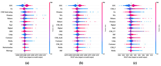
Figure 7.
SHAP summary plots for three feature sets. (a) SHAP summary plot for feature set 1; (b) SHAP summary plot for feature set 2; (c) SHAP summary plot for feature set 3.
As shown in Figure 7a, an elevated EPU leads to a rise in corporate financialization, aligning with prior scholarly work. When SA is substantial, depicted by red dots, financialization wanes (signified by lesser SHAP values), suggesting that financial constraints boost the capital available for investment in financial instruments. This discovery echoes earlier studies. The extent of financialization diminishes as Mshare increases, in line with earlier evidence. Enhanced Digital correlates with a surge in corporate financialization, in contrast to the majority of earlier studies, pointing to the necessity of delving deeper into digital transformation’s influence on financialization. A surge in Lnhp is associated with a boost in corporate financialization, corroborating earlier research. As customer concentration increases, corporate financialization decreases, which contrasts with the findings from previous studies. This difference highlights the necessity for further exploration of how customer concentration influences trends in financialization. An elevated managerial ability leads to a rise in corporate financialization, consistent with previous findings. An elevated Minwage (minimum wages) leads to a rise in corporate financialization, consistent with previous findings.
Figure 7b,c reveal that an increase in firm size (Firmsize) is associated with a reduction in corporate financialization, which aligns with most prior studies [36]. The role of marketization, however, has remained unclear in previous research, and this finding may provide valuable insights for future investigations. Several moderators, such as Top1 and HHI, show no significant effect on financialization. In contrast, higher levels of marketization are linked to lower corporate financialization.
Regarding the primary CSR dimensions, Figure 7b shows that CSR_SR (Shareholder Responsibility) and CSR_ER (Employee Responsibility) exert a positive influence on financialization, while CSR_SocR (Social Responsibility) appears to have no measurable impact. Similarly, Figure 7c demonstrates that among the secondary CSR dimensions, CSR_S (Solvency) and CSR_P (Profitability) positively affect financialization, while CSR_CV (Contribution Value) does not exhibit a clear effect.
The seemingly contradictory finding that CSR_SocR shows no linear effect warrants careful interpretation in light of existing theoretical frameworks. This apparent null effect can be reconciled with stakeholder theory and recent empirical evidence [2] through three key insights. First, as revealed in our subsequent dependence plot analysis (Section 4.6), CSR_SocR exhibits a pronounced U-shaped relationship with a threshold of approximately 10, suggesting that linear models used in previous studies may have masked these non-linear dynamics. At moderate levels of social responsibility, the positive effects (enhanced reputation, stakeholder trust) and negative effects (resource diversion from core business) may offset each other, resulting in no net linear impact. Second, this finding aligns with the emerging literature on CSR “decoupling”, where firms engage in symbolic CSR activities without substantive integration into financial strategies, potentially explaining why moderate CSR_SocR levels show limited financialization impact. Third, the interaction effects with EPU revealed in Section 4.7 indicate that CSR_SocR’s influence is highly context-dependent—during periods of high economic uncertainty, social responsibility initiatives may serve as strategic buffers that influence financialization decisions, while in stable periods, their effect diminishes. These insights contribute to the growing body of evidence suggesting that the CSR–financialization relationship is more nuanced than previously theorized, requiring non-linear modeling approaches to capture its true complexity.
Figure 8a,b compare the SHAP summary plots before and during the COVID-19 pandemic. It can be observed that Mshare (managerial ownership) experienced a change in its directional sign during the pandemic, and the sign of the controlling shareholder’s share pledge (PLD_DUM) became more pronounced during the pandemic.
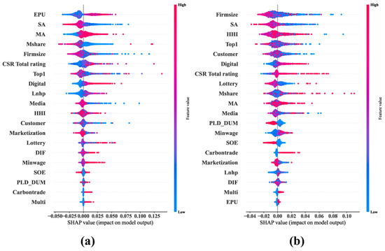
Figure 8.
SHAP summary plots before and during COVID-19. (a) SHAP summary plot before COVID-19; (b) SHAP summary plot during COVID-19.
4.6. Single-Factor Analysis Through SHAP Dependence Plots
Figure 9 illustrates the SHAP dependence plot—how the values of the variables affect the predictions (y-axis). The distribution of SHAP values for the key variables reveals a wide range of impacts on the financialization of firms, highlighting the positive and negative effects of features in the overall data.
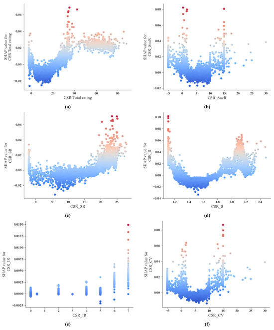
Figure 9.
SHAP dependence plots. (a) SHAP dependence plot for CSR_Total_rating; (b) SHAP dependence plot for CSR_SocR; (c) SHAP dependence plot for CSR_SR; (d) SHAP dependence plot for CSR_S; (e) SHAP dependence plot for CSR_IR; (f) SHAP dependence plot for CSR_CV.
The inflection point marks the critical value of the predictor on the x-axis, where the SHAP curve intersects the zero line on the y-axis, signifying a transition in SHAP values from positive to negative. In these visualizations, dots are color-coded to represent the magnitude of each predictor: red (or warm hues) denotes higher predictor values, while blue (or cool hues) indicates lower predictor values. The SHAP value’s sign on the y-axis reflects its impact on the target variable, with positive SHAP values corresponding to increased corporate financialization and negative values indicating reduced financialization.
The results regarding the CSR dimensions show that some of the CSR dimensions have a non-linear effect on financialization. The impact of CSR_SocR, CSR_S, CSR_SR, and CSR_CV on the enhancement of corporate financialization exhibits a U-shaped pattern, meaning that they initially decrease and then begin to increase after surpassing a certain threshold. Such a threshold is about 10 for CSR_SocR, about 1.5 for CSR_S, and about 5 for CSR_CV.
4.7. Interaction Effects Between Key Factors and Contingent Variables: SHAP Analysis
Existing research indicates that corporate financialization is a complex process influenced by multiple factors, and analyzing a single factor may not fully reveal its underlying mechanisms. To address this issue, this paper uses SHAP interaction values for visualization analysis to explore the interaction effects between key variables and common contingency factors, providing a detailed perspective on their joint impact on corporate financialization, as shown in Figure 9. Interaction effects refer to the idea that the impact of one variable depends on the value of another variable. By delving into the underlying dynamic mechanisms of these interactions, we can achieve a deeper understanding, thereby providing a richer explanation for the factors driving corporate financialization.
In the interaction plot, the x-axis is the SHAP interaction value, reflecting the strength and direction of the effect between features. The more the data points deviate from the center line, the more significant the interaction effect is. In the plot, the color of each data point reflects the value shown on the right side of the y-axis. Red points represent higher variable values, while blue points represent lower variable values. The transition from blue to red illustrates a rise in the feature values associated with the row labels. A vertical dispersion of blue and red points within a specific range suggests the presence of interaction effects. Specifically, red points positioned above blue points indicate that the contingency amplifies the primary effect. Conversely, red points located below blue points suggest that contingency weakens the primary effect. When blue and red points are closely clustered, it signifies the absence of an interaction effect.
It can also be observed from Figure 10 that when EPU is high, the impact of employee responsibility on financialization is negative. However, when the EPU is low, the impact of employee responsibility on financialization is positive. Conversely, when EPU is high, the impact of solvency on financialization is positive, whereas when EPU is low, the impact of solvency on financialization is negative. By identifying a new moderating factor, these findings suggest that research into the effects of employee responsibility and solvency on financialization will yield valuable insights. It can be inferred that the impacts of employee responsibility, minimum wages, and the cost of debt financing on financialization will be moderated by Economic Policy Uncertainty.
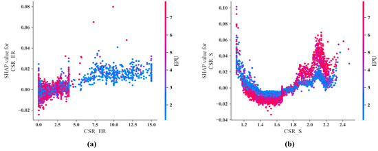
Figure 10.
SHAP interaction plots between CSR dimensions and EPU. (a) SHAP interaction plot between CSR_ER and EPU; (b) SHAP interaction plot between CSR_S and EPU.
5. Discussion
Our findings both confirm and challenge the existing research on corporate financialization. Consistent with previous studies [7], we find that EPU significantly influences financialization decisions. However, our SHAP analysis reveals that this relationship weakened dramatically during COVID-19 (68% reduction in importance), suggesting that universal uncertainty may diminish EPU’s discriminatory power—a nuance missed by traditional linear models. The U-shaped relationships discovered for CSR dimensions (CSR_SocR, CSR_S, and CSR_CV) reconcile seemingly contradictory findings in the literature. While Su & Lu [2] report positive CSR-financialization correlations and others find negative effects, our non-linear analysis shows that both can be true at different CSR levels. Specifically, moderate CSR engagement reduces financialization, while extensive CSR activities (above thresholds of 10 for CSR_SocR, 1.5 for CSR_S) increase it, suggesting a strategic shift in how CSR influences financial decisions at different engagement levels.
These findings have important theoretical implications. The discovered non-linearities challenge the linear assumptions underlying most financialization theories, suggesting that stakeholder theory and resource-based views may operate differently at various CSR intensity levels. The temporal shifts during COVID-19 indicate that financialization drivers are state-dependent rather than static, calling for dynamic theoretical frameworks. From a methodological perspective, the superior performance of XGBoost (R2 = 0.299) demonstrates the value of ensemble machine learning in capturing complex financial behaviors, while SHAP integration provides crucial interpretability without sacrificing accuracy.
For practitioners, our findings highlight critical decision thresholds. Corporate managers should recognize that CSR investments below identified thresholds may reduce financialization by signaling long-term orientation, while excessive CSR might indicate surplus resources available for financial investments. The reduced importance of traditional factors during COVID-19 suggests that strategies must adapt during crisis periods. For policymakers, the strong but changing influence of EPU underscores the importance of policy stability, while the increased importance of carbon trading policies during the pandemic suggests that environmental regulations can effectively shape corporate financial behavior even during crises.
Several limitations warrant acknowledgment. First, our analysis focuses exclusively on Chinese firms, limiting its generalizability to other institutional contexts. Second, while SHAP provides valuable insights into feature importance and interactions, it cannot establish causality [37]. Third, our one-year lag structure may not capture longer-term dynamic relationships. Fourth, some potentially relevant factors (e.g., CEO characteristics, board composition) were unavailable in our dataset. These limitations point to important future research directions.
Future studies should test our SHAP-enhanced framework across different emerging markets to assess the generalizability of the identified non-linear patterns. Developing time-varying parameter models could provide deeper insights into how feature importance evolves continuously. Combining our framework with causal inference methods could help establish causal relationships while maintaining the ability to capture non-linear patterns. Extending the framework to handle streaming data could enable real-time monitoring of corporate financialization risks, providing early warning systems for regulators. Finally, developing interactive policy simulation tools could translate our findings into actionable instruments for corporate governance and financial regulation. These extensions would advance both the methodological frontiers of interpretable machine learning in finance and practical applications for stakeholders.
Regarding the relatively low individual SHAP values observed in our analysis (with maximum values around 0.04), this pattern actually reflects the inherently multi-factorial nature of corporate financialization rather than weak predictive relationships. Three key points warrant clarification. First, corporate financialization is influenced by numerous factors beyond our 40 variables, including unobservable elements such as managerial psychology, market sentiment, and firm-specific strategic considerations, which naturally limit any single variable’s contribution. Second, the predictive power is distributed across multiple features—our analysis shows that the top 10 features cumulatively contribute approximately 68% of the model’s predictive capability, indicating that financialization emerges from the collective influence of multiple factors rather than being dominated by any single driver. Third, the discovered non-linear U-shaped relationships for several key variables (e.g., CSR_SocR, CSR_S) mean that their effects can be positive at some levels and negative at others, resulting in lower average SHAP values when aggregated across the entire sample. This distributed pattern of influence aligns with our moderate R2 of 0.299 and actually provides more nuanced insights than models dominated by one or two variables, as it reveals the complex, multi-dimensional nature of corporate financial decision-making.
Several methodological considerations warrant clarification. First, while XGBoost only marginally outperforms LightGBM (R2 = 0.299 vs. 0.252), robustness checks reveal highly consistent SHAP feature rankings between models (Spearman ρ = 0.887, p < 0.001), with 9 of 10 top features identical. This consistency validates that our key findings are robust to model choice. Second, the relatively low individual SHAP values (maximum ~0.04) reflect the multi-factorial nature of financialization rather than weak relationships. Three factors explain this pattern: (1) numerous unobservable influences beyond our 40 variables; (2) distributed predictive power, with the top 10 features cumulatively explaining 68% of predictions; and (3) U-shaped relationships where opposing effects cancel when averaged. These low values align with our moderate R2, consistent with the inherent complexity of corporate financial decisions. Finally, our Lasso-based dimensionality reduction from 40 to 27 variables effectively addresses multicollinearity (18 variables with VIF > 10) while preserving 95% of predictive power. This validates that excluded variables contributed primarily noise, supporting the development of parsimonious models for practical implementation.
6. Conclusions
This paper focuses on Chinese A-share listed companies, analyzing data from both the pre-COVID-19 period and the pandemic period to examine the impact and interactions of various factors on financialization. By employing machine learning techniques, the research evaluates the influence of CSR dimensions alongside other key variables. The SHAP was applied to identify critical factors and understand their modes of influence. Among the models tested, XGBoost demonstrated superior fitting performance and generalization capability, forming the basis for SHAP-based interpretation. To further clarify the contributions of this research, we distinguish between its technical and practical advances. From a technical perspective, this study contributes a novel SHAP-enhanced machine learning framework that integrates Lasso regularization, HO, and interpretability analysis to address the methodological challenges of high-dimensional financial prediction. This represents an advancement over traditional econometric approaches by simultaneously handling multicollinearity, capturing non-linear relationships, and providing transparent model interpretation. From a practical standpoint, the framework provides actionable tools and insights: corporate managers gain specific CSR thresholds for strategic optimization, policymakers receive evidence on how regulatory instruments dynamically influence financialization across economic cycles, and financial institutions acquire an interpretable risk assessment tool validated on over 25,000 observations.
The SHAP feature importance analysis reveals that social responsibility and shareholder responsibility are the most influential among the primary CSR indicators, while solvency, integrity, reciprocity, and contribution value stand out as key secondary CSR dimensions. In addition to CSR factors, state ownership, EPU, ownership concentration, firm size, housing prices, and carbon trading policies also emerge as important drivers of corporate financialization. Comparing the pre-pandemic (2017–2019) and pandemic (2020–2022) periods, notable shifts in factor importance are observed. The influence of ownership concentration, housing prices, managerial ownership, and EPU diminished during the pandemic, while firm size, state ownership, gambling culture, and carbon trading policies became more prominent. Further analysis shows that both primary and secondary CSR dimensions contribute positively to financialization, with these effects remaining generally consistent across periods. However, the roles of managerial ownership and controlling shareholders’ share pledges changed significantly during the pandemic. SHAP dependency plots reveal U-shaped, non-linear effects for CSR variables, while interaction plots indicate that high EPU weakens the positive effect of employee responsibility and enhances that of solvency, with reversed patterns under low EPU. These findings highlight the context-dependent and evolving nature of financialization drivers in response to external shocks.
This paper offers several practical insights for both corporate managers and policymakers. The findings underscore the importance of balancing key CSR dimensions—particularly social and shareholder responsibility—due to their non-linear U-shaped influence on financialization. Managers should avoid both neglect and overemphasis of these responsibilities to optimize financial behavior and promote sustainable development. The dynamic role of employee responsibility under varying levels of economic policy uncertainty highlights the need for adaptive CSR strategies during uncertain periods. Changes in the impact of managerial ownership during the pandemic suggest that increasing equity incentives may foster more prudent financial decisions. Additionally, firm size, solvency, and contribution value emerge as critical levers in mitigating excessive financialization. For policymakers, the complex interaction between CSR and economic policy uncertainty, as well as the significant influence of carbon trading policies, emphasizes the necessity of a stable and predictable regulatory environment. Strengthening environmental regulation and market mechanisms can guide firms toward sustainable financial practices, aligning corporate behavior with broader economic and environmental goals.
Author Contributions
Conceptualization, Y.W., Z.L. and W.W.; methodology, Y.W. and Y.L.; formal analysis, Y.W., Z.L., J.L. and Y.L.; data curation, Z.L. and J.L.; visualization, Z.L. and J.L.; investigation, Z.L.; validation, Y.W.; software, Z.L.; project administration, X.L. and W.W.; resources, Y.L.; supervision, W.W. and X.L.; writing—original draft, Y.W. and Z.L.; writing—review and editing, X.L. All authors have read and agreed to the published version of the manuscript.
Funding
This research received no external funding.
Data Availability Statement
Dataset available on request from the authors.
Conflicts of Interest
The authors declare no conflicts of interest.
References
- Klinge, T.J.; Fernandez, R.; Aalbers, M.B. Whither corporate financialization? A literature review. Geogr. Compass 2021, 15, e12588. [Google Scholar] [CrossRef]
- Su, K.; Lu, Y. The impact of corporate social responsibility on corporate financialization. Eur. J. Financ. 2023, 29, 2047–2073. [Google Scholar] [CrossRef]
- Wu, K.; Lu, Y. Corporate digital transformation and financialization: Evidence from Chinese listed firms. Financ. Res. Lett. 2023, 57, 104229. [Google Scholar] [CrossRef]
- Zhang, Z.; Su, Z.; Tong, F. Does digital transformation restrain corporate financialization? Evidence from China. Financ. Res. Lett. 2023, 56, 104152. [Google Scholar] [CrossRef]
- Si, D.K.; Zhuang, J.; Ge, X.; Yu, Y. The nexus between trade policy uncertainty and corporate financialization: Evidence from China. China Econ. Rev. 2024, 84, 102113. [Google Scholar] [CrossRef]
- Sui, B.; Yao, L. The impact of digital transformation on corporate financialization: The mediating effect of green technology innovation. Innov. Green Dev. 2023, 2, 100032. [Google Scholar] [CrossRef]
- Cheng, Z.; Masron, T.A. Does economic policy uncertainty exacerbate corporate financialization? Evidence from China. Appl. Econ. Lett. 2024, 31, 1028–1036. [Google Scholar] [CrossRef]
- Du, P.; Zheng, Y.; Wang, S. The minimum wage and the financialization of firms: Evidence from China. China Econ. Rev. 2022, 76, 101870. [Google Scholar] [CrossRef]
- Jiang, F.; Shen, Y.; Cai, X. Can multiple blockholders restrain corporate financialization? Pac.-Basin Financ. J. 2022, 75, 101827. [Google Scholar] [CrossRef]
- Ma, X.; Xu, Q. The impact of carbon emissions trading policy on carbon emission of China’s power industry: Mechanism and spatial spillover effect. Environ. Sci. Pollut. Res. 2023, 30, 74207–74222. [Google Scholar] [CrossRef]
- Wang, H.; Sun, K.; Xu, S. Does housing boom boost corporate financialization?—Evidence from China. Emerg. Mark. Financ. Trade 2023, 59, 1655–1667. [Google Scholar] [CrossRef]
- Cao, W.; Chen, C.; Jiang, D.; Li, W.; Zhang, Y. Industrial policy and non-financial corporations’ financialization: Evidence from China. Eur. J. Financ. 2022, 28, 397–415. [Google Scholar] [CrossRef]
- Zhang, X.; Zheng, X. Does carbon emission trading policy induce financialization of non-financial firms? Evidence from China. Energy Econ. 2024, 131, 107316. [Google Scholar] [CrossRef]
- Liu, H.; Pan, H. Reducing carbon emissions at the expense of firm physical capital investments and growing financialization? Impacts of carbon trading policy from a regression discontinuity design. J. Environ. Manag. 2024, 356, 120577. [Google Scholar] [CrossRef] [PubMed]
- Su, K.; Zhao, Y.; Wang, Y. Customer concentration and corporate financialization: Evidence from non-financial firms in China. Res. Int. Bus. Financ. 2024, 68, 102159. [Google Scholar] [CrossRef]
- Zhong, H.; Al-Duais, Z.A.M.; Peng, B. The impact of idiosyncratic risk on corporate financialization—Evidence from China. Int. Rev. Financ. Anal. 2023, 86, 102491. [Google Scholar] [CrossRef]
- Hou, Q.; Tang, X.; Teng, M. Labor costs and financialization of real sectors in emerging markets. Pac.-Basin Financ. J. 2021, 67, 101547. [Google Scholar] [CrossRef]
- Tang, Y.; Wang, L.; Shu, H. Tax reduction and the financialization of real enterprises: Evidence from China’s VAT reform. Int. Rev. Econ. Financ. 2024, 92, 835–850. [Google Scholar] [CrossRef]
- Zhang, Y.; Zhang, H.; Yang, L.; Xu, P. Managerial ownership and corporate financialization. Financ. Res. Lett. 2023, 58, 104682. [Google Scholar] [CrossRef]
- Gao, R.; Cui, S.; Wang, Y.; Xu, W. Predicting financial distress in high-dimensional imbalanced datasets: A multi-heterogeneous self-paced ensemble learning framework. Financ. Innov. 2025, 11, 50. [Google Scholar] [CrossRef]
- Elena, D.; Hué, S.; Hurlin, C.; Tokpavi, S. Machine learning for credit scoring: Improving logistic regression with non-linear decision-tree effects. Eur. J. Oper. Res. 2022, 297, 1178–1192. [Google Scholar]
- Liu, J.; Liu, Z.; Li, Q.; Kong, W.; Li, X. Multi-Domain Controversial Text Detection Based on a Machine Learning and Deep Learning Stacked Ensemble. Mathematics 2025, 13, 1529. [Google Scholar] [CrossRef]
- Li, X.; Wang, X.; Kong, T.; Zheng, J.; Luo, M. From bitcoin to solana–innovating blockchain towards enterprise applications. In Proceedings of the International Conference on Blockchain, Virtual Event, 10–14 December 2021; Springer International Publishing: Berlin/Heidelberg, Germany; pp. 74–100. [Google Scholar]
- Li, X.; Sigov, A.; Ratkin, L.; Ivanov, L.A.; Li, L. Artificial intelligence applications in finance: A survey. J. Manag. Anal. 2023, 10, 676–692. [Google Scholar] [CrossRef]
- Campisi, G.; Muzzioli, S.; De Baets, B. A comparison of machine learning methods for predicting the direction of the US stock market on the basis of volatility indices. Int. J. Forecast. 2024, 40, 869–880. [Google Scholar] [CrossRef]
- Jones, S.; Moser, W.J.; Wieland, M.M. Machine learning and the prediction of changes in profitability. Contemp. Account. Res. 2023, 40, 2643–2672. [Google Scholar] [CrossRef]
- Li, Z. Extracting spatial effects from machine learning model using local interpretation method: An example of SHAP and XGBoost. Comput. Environ. Urban Syst. 2022, 96, 101845. [Google Scholar] [CrossRef]
- Martins, T.; De Almeida, A.M.; Cardoso, E.; Nunes, L. Explainable artificial intelligence (XAI): A systematic literature review on taxonomies and applications in finance. IEEE Access 2023, 12, 618–629. [Google Scholar] [CrossRef]
- Wang, S.; Meng, H.; Chen, Z. Exploring the links between bank competition, economic policy uncertainty, and corporate financialization. Financ. Res. Lett. 2025, 78, 107100. [Google Scholar] [CrossRef]
- Wang, M.; Mohd Nor, N.; Abdul Rahim, N.; Khan, F.; Zhou, Z. Trade policy uncertainty and corporate financialization: Strategic implications for non-financial firms in China. Cogent Econ. Financ. 2025, 13, 2460078. [Google Scholar] [CrossRef]
- Shen, J.; Xu, M.; Liu, X.; Zhao, Y. Active adaptation or short-run profit pursuing? Carbon emissions trading and corporate financialization: Evidence from Chinese listed companies. Environ. Dev. Sustain. 2024, 1–18. [Google Scholar] [CrossRef]
- Gao, C.; Zhang, S. ESG performance and corporate financialization: A dual perspective of risk management and value creation. Financ. Res. Lett. 2025, 71, 106442. [Google Scholar] [CrossRef]
- Xu, S. Corporate social responsibility and financialization: Is CSR used as a financial tool? Eur. Manag. Rev. 2025, 1–19. [Google Scholar] [CrossRef]
- Zhang, J.; Ma, X.; Zhang, J.; Sun, D.; Zhou, X.; Mi, C.; Wen, H. Insights into geospatial heterogeneity of landslide susceptibility based on the SHAP-XGBoost model. J. Environ. Manag. 2023, 332, 117357. [Google Scholar] [CrossRef] [PubMed]
- Sun, Y.; Qu, Z.; Liu, Z.; Li, X. Hierarchical Multi-Scale Decomposition and Deep Learning Ensemble Framework for Enhanced Carbon Emission Prediction. Mathematics 2025, 13, 1924. [Google Scholar] [CrossRef]
- Amiri, M.H.; Hashjin, N.M.; Montazeri, M.; Mirjalili, S.; Khodadadi, N. Hippopotamus optimization algorithm: A novel nature-inspired optimization algorithm. Sci. Rep. 2024, 14, 5032. [Google Scholar] [CrossRef] [PubMed]
- Zhang, Y.; Guo, J.; Ding, X.; Tang, Z.; Wang, T.; Wu, W.; Jia, W. Optimizing Communication Efficiency through Training Potential in Multi-Modal Federated Learning. ACM Trans. Internet Technol. 2025. [Google Scholar] [CrossRef]


Disclaimer/Publisher’s Note: The statements, opinions and data contained in all publications are solely those of the individual author(s) and contributor(s) and not of MDPI and/or the editor(s). MDPI and/or the editor(s) disclaim responsibility for any injury to people or property resulting from any ideas, methods, instructions or products referred to in the content. |
© 2025 by the authors. Licensee MDPI, Basel, Switzerland. This article is an open access article distributed under the terms and conditions of the Creative Commons Attribution (CC BY) license (https://creativecommons.org/licenses/by/4.0/).