Abstract
This paper develops an analytical pricing formula for vulnerable options with stochastic volatility under a two-factor stochastic interest rate model. We consider the underlying asset price following the Heston stochastic volatility model, while the interest rate is modeled as the sum of two processes. Using the joint characteristic function approach and measure change techniques, we derive an explicit pricing formula for a vulnerable European option. We also conduct numerical experiments to examine the effects of various model parameters on option values. This study provides a more realistic framework for pricing OTC derivatives by incorporating credit risk, stochastic volatility, and stochastic interest rates simultaneously.
Keywords:
vulnerable option; stochastic interest rate; stochastic volatility; characteristic function MSC:
91G20; 91G40
1. Introduction
Over-the-counter (OTC) options have grown significantly in recent years, with numerous corporations regularly entering into these derivative contracts with investors. However, after the global financial crisis of 2007–2008, investors have increasingly acknowledged the importance of counterparty credit risk in OTC trading. OTC contracts have no guarantee, thus immediately exposing option holders to potential losses if the counterparty defaults. Such financial derivatives, known as ‘vulnerable options’, entitle holders to claim the issuer’s assets if the issuer defaults on payment obligations.
An initial study by Johnson and Stulz [1] incorporated credit risk into European option pricing within a Black–Scholes framework, assuming the option as the issuer’s sole liability. Klein [2] further developed this model by considering additional liabilities of the option issuer and allowing correlation between the issuer’s assets and the underlying assets. Extensions of Klein’s approach include incorporating liability from written options into default thresholds, as discussed in several extensions. Klein and Inglis [3] and Liao and Huang [4] incorporated stochastic interest rates, enhancing the realism of vulnerable option pricing frameworks. Additional studies, such as those by Tian et al. [5], Fard [6], Han [7], and Wang et al. [8], investigated the pricing formulas for vulnerable options within jump-diffusion environments. Recently, many researchers have developed pricing models for vulnerable options with stochastic liquidity risk [9,10,11,12,13].
Many existing studies assumed constant volatility in the underlying asset price, which contradicts observable market patterns such as volatility clustering, volatility smiles, and leptokurtic return distributions. Recent advances in mathematical finance have further enriched the option pricing literature. For instance, fractional stochastic models have been proposed to capture long-range dependence in financial markets [14], and the synchronization and chaos suppression techniques in financial models [15] have provided new insights into managing complex dynamics in option pricing. These developments motivate our current work on integrating multiple sources of risk in a framework.
In order to address this, research efforts to develop vulnerable option pricing models have used stochastic volatility models. Lee et al. [16] provided explicit solutions for vulnerable options in a Heston framework [17], and Wang et al. [18] introduced CIR processes to describe stochastic volatility dynamics in pricing model of vulnerable option. Me et al. [19] developed processes for pricing vulnerable options with both stochastic volatility and interest rates. In addition, Jeon et al. [20] derived the analytical pricing formula of the vulnerable exchange option using the asymptotic expansion. Motivated by these studies, we also develop the pricing model of vulnerable options with stochastic volatility. Specifically, we investigate the pricing for vulnerable options by incorporating a two-factor stochastic interest rate model when the underlying assets follow the Heston model.
It should be noted that the vulnerable options literature under the structrual model have developed along two streams: the Klein framework and the barrier option approach based on Black and Cox [21]. The latter models default through barrier conditions, as seen in Escobar et al. [22] and Gotz et al. [23]. In this paper, we follow the Klein framework. While the existing literature has made significant progress in vulnerable option pricing, there remain important gaps that our paper addresses. Although Scott [24] introduced a two-factor interest rate model for option pricing, this framework has not been extended to vulnerable options with stochastic volatility. The two-factor structure is particularly important for capturing both term structure dynamics and the correlation between interest rates and volatility; however, most vulnerable option models adopt single-factor interest rate processes. This paper overcomes these gaps by developing the first model for vulnerable option pricing that considers both two-factor stochastic interest rates and correlated stochastic volatility. Specifically, we extend the stochastic volatility framework to a case in which both the underlying asset and the issuer’s asset share a common volatility factor, while the stochastic interest rate follows a two-factor model defined as the sum of two CIR processes.
While significant models have been used for vulnerable option pricing, no previous studies have addressed the particular structure of two-factor stochastic interest rates combined with stochastic volatility for both the underlying and issuer’s assets. This is important because real markets exhibit both complex interest rate dynamics and increased asset correlations during stress periods. Our study contributes to this by proposing an analytical solution for vulnerable options in this realistic but previously unstudied model.
The main contributions of this paper are fourfold. First, we derive the joint characteristic function for a system where asset prices follow correlated processes with stochastic volatility under a two-factor interest rate model. Second, we develop an analytical pricing formula for the vulnerable option price using measure change techniques and joint characteristic function. Third, through extensive numerical analysis, we present an interesting differences sensitivity: the first interest rate factor, which affects both discounting and volatility dynamics, has a substantially larger impact on option values than the second factor, which just impacts discounting. It has significant implications for risk management and hedging strategies. Finally, we verify our analytical formulas through Monte Carlo simulations, demonstrating high precision. This demonstrates that our formula is accurate and practical.
The rest of the paper is organized as follows. In Section 2, the stochastic volatility model and two-factor interest rate model are briefly described. In Section 3, we derive the joint characteristic function of underlying assets, and provide an analytic pricing formula for vulnerable options under the proposed model. Section 4 presents the numerical results. Section 5 concludes the paper.
2. Model Formulation
We consider as a complete probability space, with a filtration satisfying the usual condition and Q being a risk-neutral measure. Under the measure Q, as in Lee et al. [16], we assume that the dynamics of two risky assets and are given by the following:
where the parameters mean the following:
- : volatility parameters of the underlying asset and issuer’s asset, respectively;
- : volatility of volatility parameters;
- : mean reversion speeds;
- : long-term mean levels of the factors;
- : standard Brownian motions.
Here, as in Scott [24], we define a two-factor stochastic interest rate as
This allows us to capture both the term structure dynamics (through ) and the volatility–interest rate correlation (through ). Moreoever, the correlation between the interest rate and volatility is
and the correlation between the Brownian motions are
Based on the model for underlying assets with two-factor stochastic interest rates and stochastic volatility, we examine the valuation of options under default risk.
3. Valuation of Vulnerable Options
In this section, we investigate the pricing of vulnerable options under the proposed model which was introduced in the previous section. To obtain an analytical pricing formula of option, we use the characterisitic function of the underlying assets. Let and . The joint characteristic function is defined as
where T is maturity and . The explicit form of characteristic function is provided in the following Lemma.
Lemma 1.
The joint characteristic function of and has the following form.
where
and
Proof.
We employ the Feynman–Kac theorem to derive the characteristic function. The proof proceeds in three steps: (1) establishing the PDE, (2) proposing an exponential–affine solution form, and (3) solving the resulting ODEs.
The characteristic function satisfies the following PDE:
where is the infinitesimal generator of the state processes and . Specifically, the Feynman–Kac theorem gives the following PDE for
with the terminal condition .
We assume that the PDE has an exponential–affine solution of the form
where , the functions , , and are to be determined, and the initial conditions , and . The required partial derivatives are as follows:
Substituting these into the PDE and dividing by yields an equation.
We collect terms based on the powers of , , and the constant term, and set each collection to zero.
For , we have
Rearranging for gives the correct ODE:
Substituting the definitions of and yields
For , we have
Rearranging for gives the correct ODE:
Using the definition of , this simplifies to
For constant terms, we have
The equations for and are standard Riccati equations. These equations have finite solutions for when and satisfy and . Under the Feller conditions and , these requirements are satisfied for all in the integration domain.
With the initial conditions and , the solutions are as follows:
The solution to a Riccati equation of the form with is given by
Applying this to our ODEs for and yields the results presented in the Lemma.
In addtion, the coefficient is found by integrating the solutions for and from 0 to .
The definite integral of the Riccati solution is a known result. For an equation , the integral is
Applying this formula to our integrals for B and C (with their respective coefficients ) and multiplying by and gives the expression for stated in the Lemma. This completes the proof. □
From Lemma 1, we can obtain the explicit pricing formula of a vulnerable European option under the structural model, using the model proposed in the previous section. We now consider a vulnerable option with maturity T. Under the structural model, the default event occurs if the option issuer’s asset falls below the default boundary D. Then, the option price at time 0 under measure Q is given by
where K is the strike price, is the deadweight cost, and is the indicator function. Using the characteristic function in Lemma 1, we can obtain the analytic pricing formula of vulnerable option under the proposed model shown in the following Theorem.
Theorem 1.
The price C of a vulnerable European call option at time 0 under the proposed model is given by
where each term is defined as
where , and the probability functions and are defined by
respectively. The characteristic functions used in the formulas above are expressed using the joint characteristic function Ψ as follows:
where the joint characteristic function Ψ is defined in Lemma 1 of the paper.
Proof.
Under the risk-neutral measure Q, the price of the vulnerable European call option at time is given by
where
To calculate , and using the measure change technique, we define the following Radon–Nikodym derivatives:
Then, under new measures, the expectations are represented by
According to the relationship between the distribution function and the characteristic function , it holds that
For , we have
However, for direct computation, we use
We now consider the characteristic fucntion under measure .
Since , the characteristic fucntion under measure is defined by
Similarly, we obtain the following:
We rewrite this as
4. Numerical Examples
In this section, we present numerical examples to examine the behavior of vulnerable option prices under a two-factor stochastic interest rate model with stochastic volatility. We investigate how various model parameters affect option values and provide insights into the pricing dynamics of vulnerable options.
Table 1 presents the base case parameters used in our numerical analysis. The parameters in Table 1 are chosen based on previous studies. Specifically, we adopt parameter values following the works of Lee et al. [16] and Scott [24]. The higher mean reversion speed reflects faster adjustment in short-term volatility, while represents slower long-term interest rate dynamics. The long-term means correspond to 20% annualized volatility, typical for equity markets. The correlation captures the negative relationship between asset values during market stress. We also implement a Monte Carlo simulation with time step and 50,000 sample paths to verify our analytical pricing formula. To ensure non-negative values in the CIR processes, we employ the absorption fix in the Euler–Maruyama scheme: , where represents independent standard normal random variables. The results are presented in Table 2.

Table 1.
Parameter values of options in the base case.

Table 2.
Monte Carlo simulation results for vulnerable option pricing.
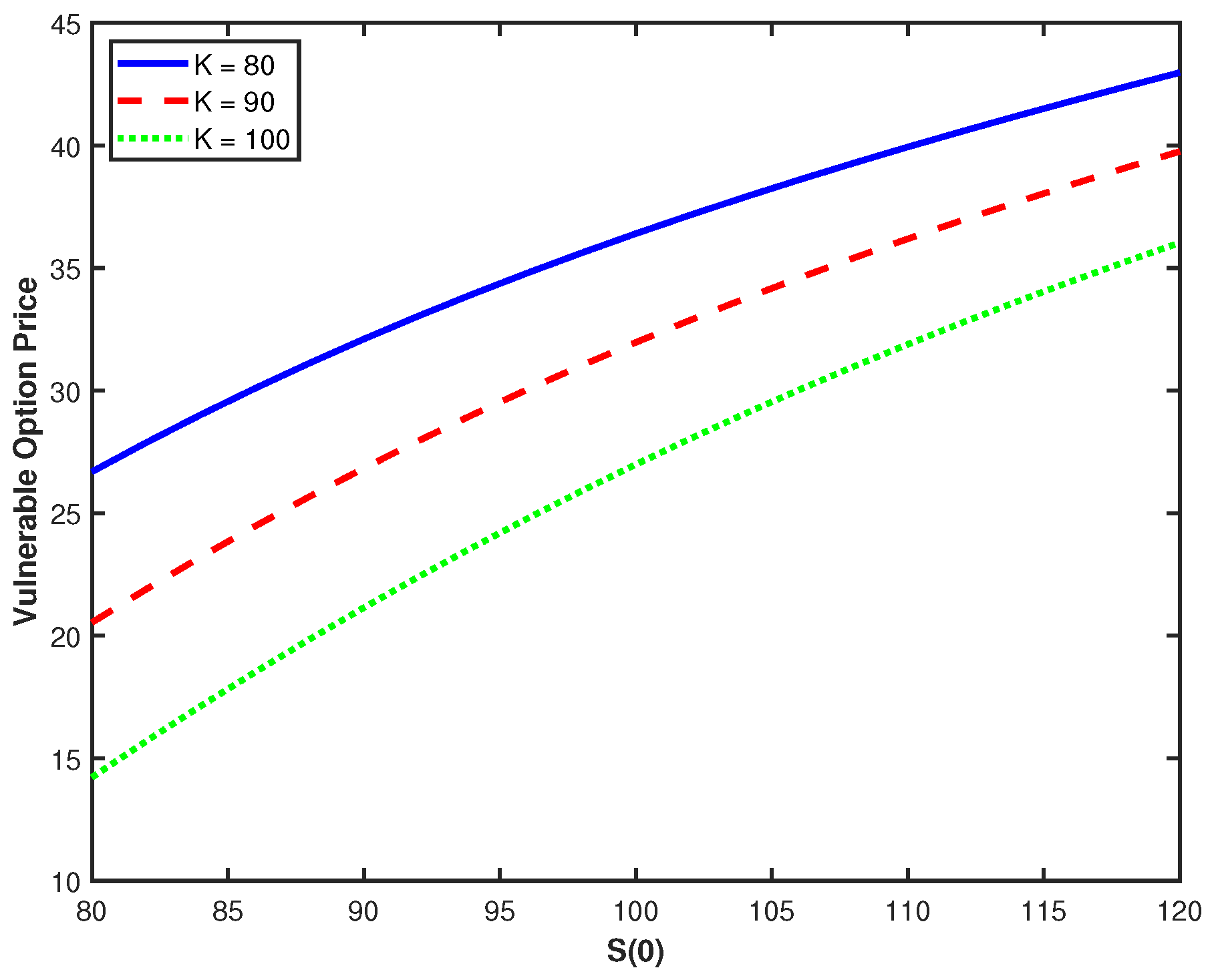
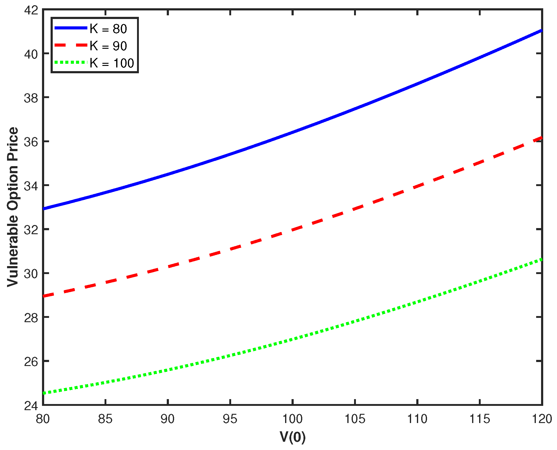
Figure 1 illustrates the relationship between the underlying asset price and vulnerable option values for three different strike prices (). As expected, option values increase monotonically with the underlying asset price. Interestingly, the vertical distance between curves decreases as S(0) increases. Figure 2 examines the effect of the issuer’s asset value on option prices, revealing an exponential growth pattern. The relationship shows that option values increase dramatically as rises, with the rate of increase accelerating at higher issuer asset values. As the issuer’s assets increase relative to the default boundary, the probability of default decreases exponentially, leading to a corresponding exponential increase in option value. The convexity of option value in relation to reflects the fundamental nature of option payoffs, whereas exponential growth with captures the rapidly decreasing default probability.
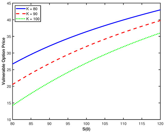
Figure 1.
Option prices against with different K.
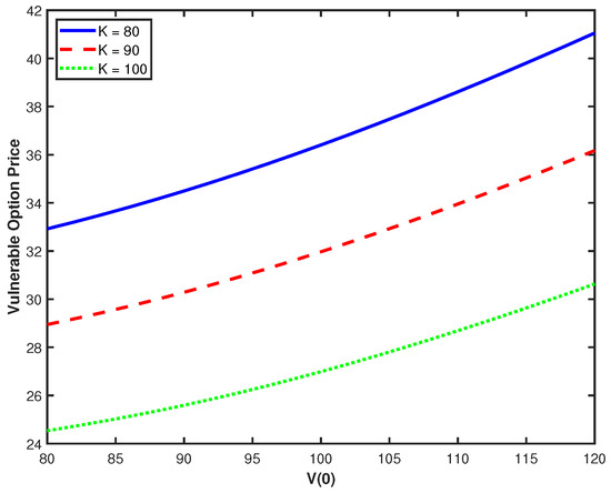
Figure 2.
Option prices against with different K.
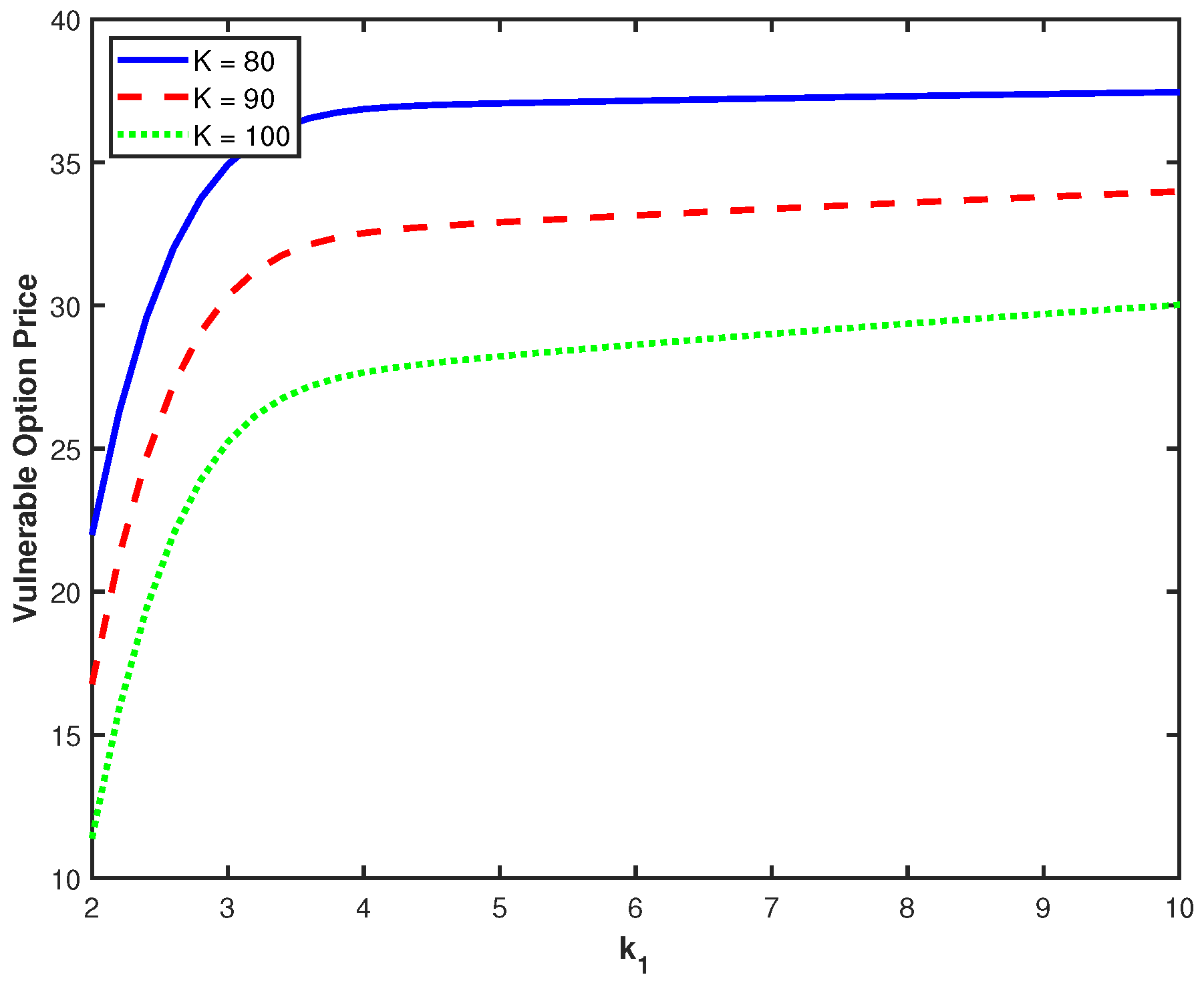
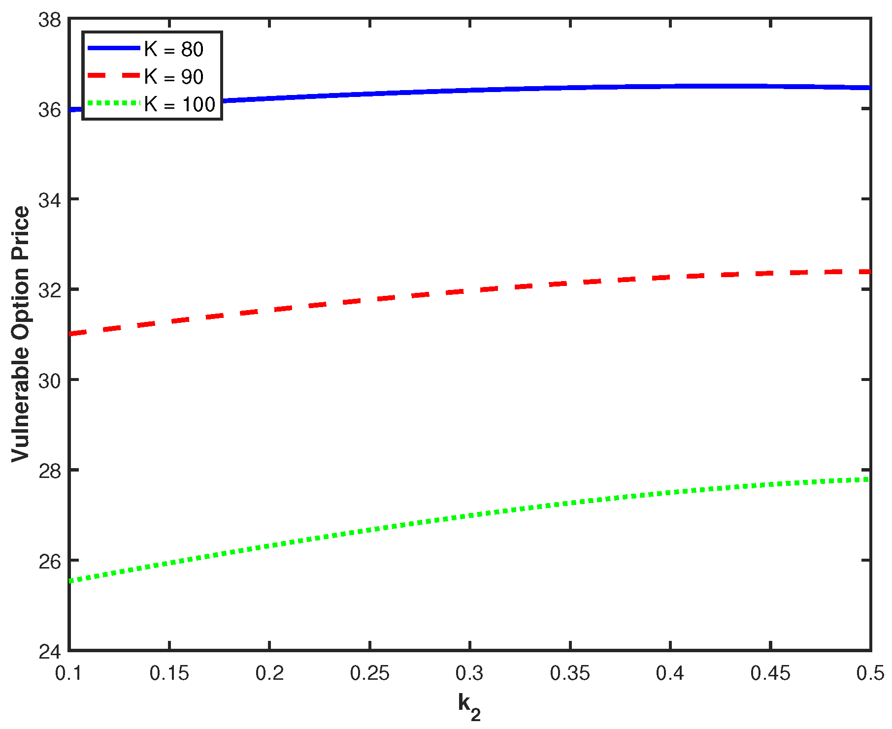
Figure 3 and Figure 4 explore the effects of mean reversion parameters and on option prices. The sensitivity to (Figure 3) shows that faster mean reversion in the first interest rate factor leads to higher option values. This positive relationship suggests that greater stability in interest rates (faster mean reversion) enhances option values by reducing uncertainty in the discount factor. However, we can also observe an interesting convergence phenomenon for larger . That is, the marginal impact of increasing diminishes significantly beyond a certain threshold, and these further increases provide decreasing benefits since mean reversion becomes sufficiently rapid. In contrast, the impact of (Figure 4) is relatively modest, with option values showing minimal sensitivity to changes in the second factor’s mean reversion speed. The comparatively flat curves show that has little influence on option valuation within the parameter range considered. This difference in response to the two factors shows that the first component has a greater impact on option valuation, most likely due to its direct relationship to the stochastic volatility process. This provides important insights for model calibration and risk management: parameters governing volatility dynamics require more careful estimation than those affecting only interest rates.
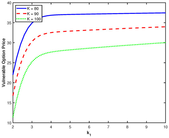
Figure 3.
Option prices against with different K.
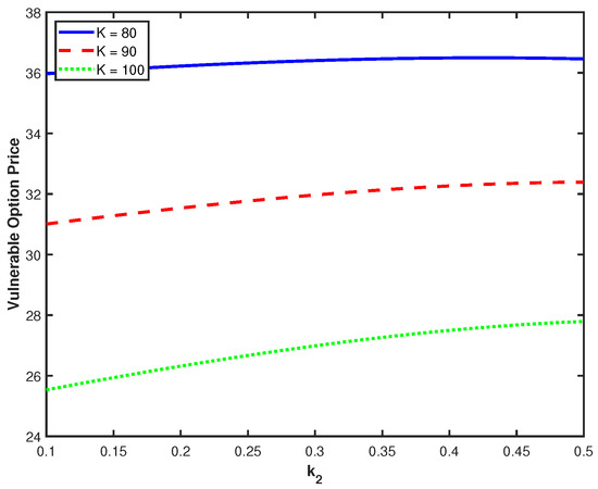
Figure 4.
Option prices against with different K.
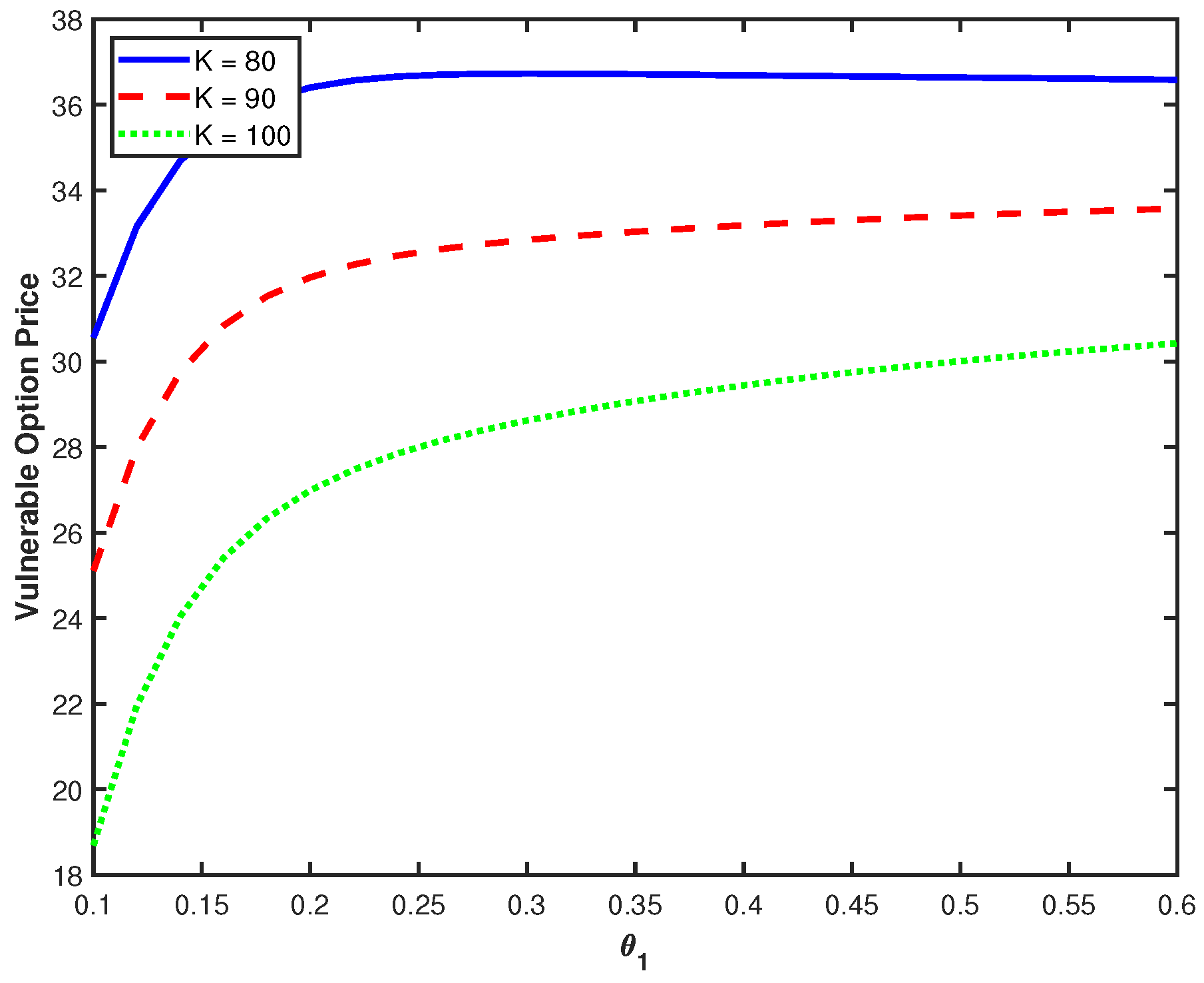
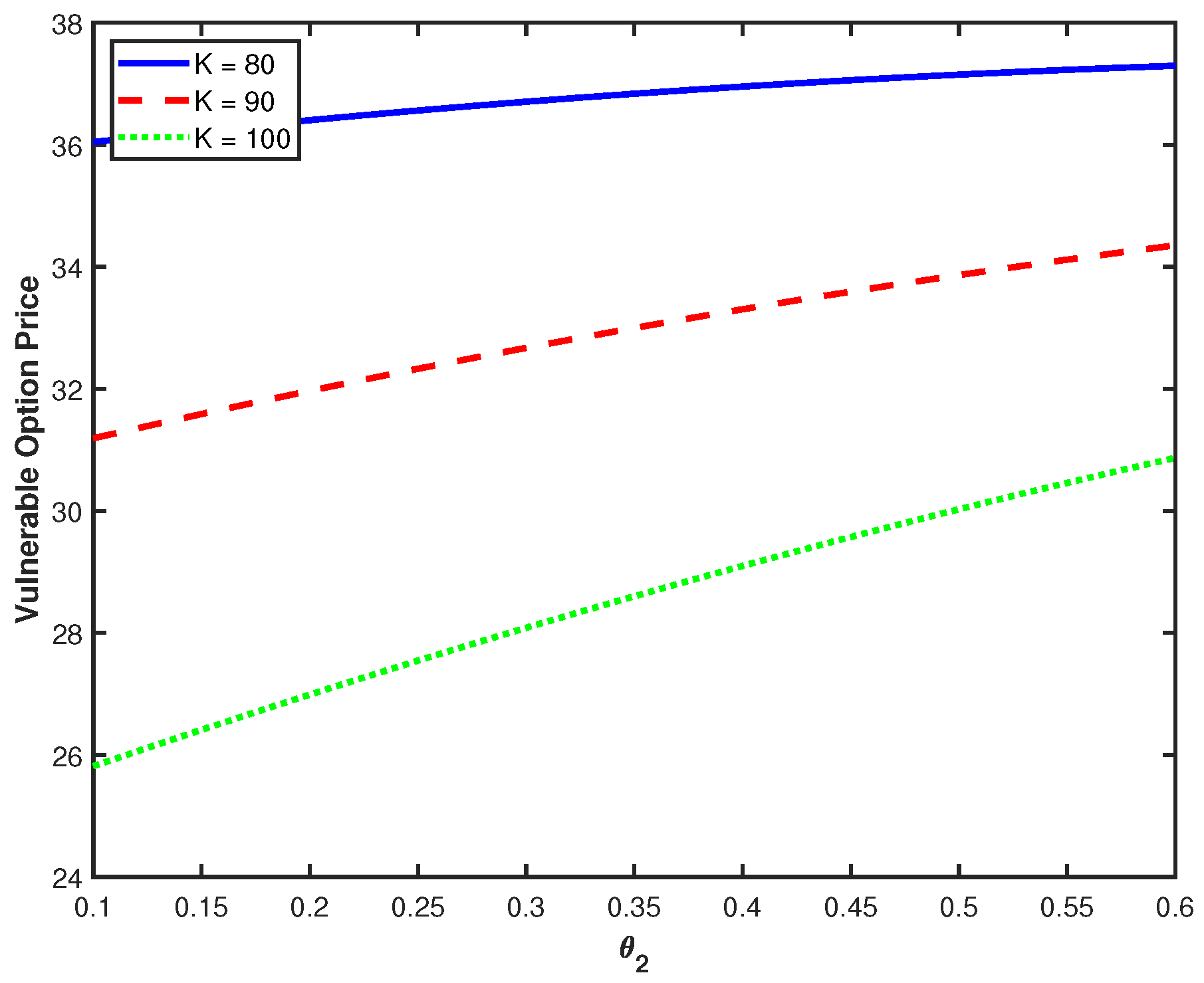
Figure 5 shows the impact of on option values, revealing a pronounced positive relationship. We observe a distinctive pattern where option values exhibit a sharp increase at low values (particularly between 0.1 and 0.3) followed by a pronounced flattening as continues to increase. As increases from low levels, it establishes a more stable floor for the volatility process, resulting in improved price stability and higher option values. The flattening of the curves indicates that once a reasonable volatility floor is established, further increases provide decreasing returns. Figure 6 presents the sensitivity to , the long-term mean of the second interest rate factor. The relationship here is notably different from , showing an approximately linear and much more modest increase. The near-linear relationship and limited sensitivity indicate that the second factor plays a secondary role in option valuation. This differential sensitivity to and reflects the asymmetric structure of our model. While both factors contribute to the interest rate , only affects the asset volatility dynamics through Equations (1) and (2). Consequently, influences option values through multiple channels—discount rates, volatility levels, and volatility of volatility—while affects only the discount rate component.
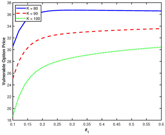
Figure 5.
Option prices against with different K.

Figure 6.
Option prices against with different K.
Our numerical analysis reveals several important economic insights. The dramatic difference in sensitivities to the two factor parameters demonstrates that the coupling between volatility and interest rates through creates first-order effects, while pure interest rate dynamics have second-order impacts. This suggests that models separating volatility and interest rate dynamics may miss important interaction effects. Furthermore, the exponential sensitivity to issuer asset value, combined with the significant impact of volatility parameters, indicates that credit risk and market risk are intrinsically connected in vulnerable option valuation. During market stress, when volatility increases, the higher probability of counterparty default causes the option value decrease. These findings have significant implications for risk management and hedging of OTC derivatives, implying that volatility and credit risk should be managed simultaneously rather than separately.
5. Concluding Remarks
In this paper, we have developed an analytical pricing approach for vulnerable options under an intergrated model that incorporates stochastic volatility and a two-factor stochastic interest rate structure. By combining the Heston stochastic volatility model with a two-factor interest rate model, we provide a more realistic approach to valuing options with counterparty credit risk in OTC markets.
To obtain the pricing formula, we derive the joint characteristic function for the underlying asset and issuer’s asset under the proposed model. Using the joint characteristic function and measure change techniques, we present explicit pricing formulas for vulnerable European options based on the probabilistic approach. The option price is decomposed into four components that can be efficiently computed through numerical integration. We also conduct several numerical experiments to investigate the sensitivities of option values to various model parameters. The numerical results show several insights into the behavior of vulnerable option prices under the proposed model. The results confirmed that option values increase with both the underlying asset’s price and the issuer’s asset value, as expected. Significantly, the results revealed an asymmetric sensitivity to the two components of the stochastic interest rate. Parameters related to the first interest rate factor, which is directly linked to the asset’s volatility dynamics, have a substantial impact on the option price. In contrast, we find that the parameters of the second interest rate factor, which only affects the discount rate, have a comparatively modest influence on the option’s value.
Author Contributions
J.J. and G.K. designed the model; J.J. and G.K. contributed to the analysis of the mathematical model; J.J. proved the propositions in the paper; J.J. and G.K. wrote the paper. All authors have read and agreed to the manuscript.
Funding
This research was supported by Seoul National University of Science and Technology.
Data Availability Statement
The original contributions presented in the study are included in the article; further inquiries can be directed to the corresponding author(s).
Conflicts of Interest
The authors declare no conflicts of interest.
References
- Johnson, H.; Stulz, R. The pricing of options with default risk. J. Financ. 1987, 42, 267–280. [Google Scholar] [CrossRef]
- Klein, P. Pricing Black-Scholes options with correlated credit risk. J. Bank. Financ. 1996, 20, 1211–1229. [Google Scholar] [CrossRef]
- Klein, P.; Inglis, M. Valuation of European options subject to financial distress and interest rate risk. J. Deriv. 1999, 6, 44–56. [Google Scholar] [CrossRef]
- Liao, S.L.; Huang, H.H. Pricing Black–Scholes options with correlated interest rate risk and credit risk: An extension. Quant. Financ. 2005, 5, 443–457. [Google Scholar] [CrossRef]
- Tian, L.; Wang, G.; Wang, X.; Wang, Y. Pricing vulnerable options with correlated credit risk under jump-diffusion processes. J. Futur. Mark. 2014, 34, 957–979. [Google Scholar] [CrossRef]
- Fard, F.A. Analytical pricing of vulnerable options under a generalized jump–diffusion model. Insur. Math. Econ. 2015, 60, 19–28. [Google Scholar] [CrossRef]
- Han, X. Valuation of vulnerable options under the double exponential jump model with stochastic volatility. Probab. Eng. Informational Sci. 2019, 33, 81–104. [Google Scholar] [CrossRef]
- Wang, X.; Song, S.; Wang, Y. The valuation of power exchange options with counterparty risk and jump risk. J. Futur. Mark. 2017, 37, 499–521. [Google Scholar] [CrossRef]
- Pan, Y.; Tang, D.; Wang, X. Valuation of vulnerable European options with market liquidity risk. Probab. Eng. Informational Sci. 2024, 38, 65–81. [Google Scholar] [CrossRef]
- He, X.J.; Pasricha, P.; Lu, T.; Lin, S. Vulnerable options with regime switching and stochastic liquidity. Q. Rev. Econ. Financ. 2024, 98, 101930. [Google Scholar] [CrossRef]
- Wang, B.; Wang, X.; Zhao, M. Valuing Vulnerable Basket Options with Stochastic Liquidity Risk in Reduced-form Models. Comput. Econ. 2024, 1–17. [Google Scholar] [CrossRef]
- Jeon, J.; Kim, G. Analytically Pricing a Vulnerable Option under a Stochastic Liquidity Risk Model with Stochastic Volatility. Mathematics 2024, 12, 2642. [Google Scholar] [CrossRef]
- He, X.J.; Huang, S.D.; Lin, S. A closed-form solution for pricing European-style options under the Heston model with credit and liquidity risks. Commun. Nonlinear Sci. Numer. Simul. 2025, 143, 108595. [Google Scholar] [CrossRef]
- Sahebi Fard, H.; Dastranj, E.; Jajarmi, A. A Novel Fractional Stochastic Model Equipped with ψ-Caputo Fractional Derivative in a Financial Market. Math. Methods Appl. Sci. 2025, 48, 9653–9661. [Google Scholar] [CrossRef]
- Jajarmi, A.; Hajipour, M.; Baleanu, D. New aspects of the adaptive synchronization and hyperchaos suppression of a financial model. Chaos Solitons Fractals 2017, 99, 285–296. [Google Scholar] [CrossRef]
- Lee, M.K.; Yang, S.J.; Kim, J.H. A closed form solution for vulnerable options with Heston’s stochastic volatility. Chaos Solitons Fractals 2016, 86, 23–27. [Google Scholar] [CrossRef]
- Heston, S.L. A closed-form solution for options with stochastic volatility with applications to bond and currency options. Rev. Financ. Stud. 1993, 6, 327–343. [Google Scholar] [CrossRef]
- Wang, G.; Wang, X.; Zhou, K. Pricing vulnerable options with stochastic volatility. Phys. A Stat. Mech. Its Appl. 2017, 485, 91–103. [Google Scholar] [CrossRef]
- Ma, Y.; Pan, D.; Shrestha, K.; Xu, W. Pricing and hedging foreign equity options under Hawkes jump–diffusion processes. Phys. A Stat. Mech. Its Appl. 2020, 537, 122645. [Google Scholar] [CrossRef]
- Jeon, J.; Huh, J.; Kim, G. An analytical approach to the pricing of an exchange option with default risk under a stochastic volatility model. Adv. Contin. Discret. Model. 2023, 2023, 37. [Google Scholar] [CrossRef]
- Black, F.; Cox, J.C. Valuing corporate securities: Some effects of bond indenture provisions. J. Financ. 1976, 31, 351–367. [Google Scholar] [CrossRef]
- Escobar, M.; Friederich, T.; Krayzler, M.; Seco, L.; Zagst, R. Structural credit modeling under stochastic volatility. Int. J. Stat. Probab. 2012, 1, 20. [Google Scholar] [CrossRef]
- Götz, B.; Escobar, M.; Zagst, R. Closed-form pricing of two-asset barrier options with stochastic covariance. Appl. Math. Financ. 2014, 21, 363–397. [Google Scholar] [CrossRef]
- Scott, L.O. Pricing stock options in a jump-diffusion model with stochastic volatility and interest rates: Applications of Fourier inversion methods. Math. Financ. 1997, 7, 413–426. [Google Scholar] [CrossRef]
Disclaimer/Publisher’s Note: The statements, opinions and data contained in all publications are solely those of the individual author(s) and contributor(s) and not of MDPI and/or the editor(s). MDPI and/or the editor(s) disclaim responsibility for any injury to people or property resulting from any ideas, methods, instructions or products referred to in the content. |
© 2025 by the authors. Licensee MDPI, Basel, Switzerland. This article is an open access article distributed under the terms and conditions of the Creative Commons Attribution (CC BY) license (https://creativecommons.org/licenses/by/4.0/).

