Identification and Estimation in Linear Models with Endogeneity Through Time-Varying Volatility

Abstract

This paper proposes a novel control function approach to identify and estimate linear models with endogenous variables in the absence of valid instrumental variables. The identification strategy exploits time-varying volatility to address the multicollinearity problem that arises in conventional control function methods when instruments are weak. We establish the identification conditions and show that the proposed method is $\sqrt{T}$-consistent and asymptotically normal. We apply the proposed approach to estimate the elasticity of intertemporal substitution, a key parameter in macroeconomics. Using quarterly data on aggregate stock returns across eleven countries, we find that the data exhibit substantial time variation in volatility, supporting the identifying assumptions. The proposed method yields confidence intervals that are broadly consistent with the general findings in the literature and are substantially narrower than those obtained using weak-instrument robust methods.

1. Introduction

In the linear regression framework, the instrumental variable (IV) is one of the most widely applied methods to tackle endogeneity in empirical research. A valid IV must satisfy three conditions: (1) it must be excluded from the structural equation; (2) it must be uncorrelated with the structural error term; (3) it must be strongly correlated with the endogenous regressors. If any of these conditions fail, the conventional IV estimator will produce biased and inconsistent results. In many empirical applications, it is often debatable whether the exclusion and the orthogonality conditions hold. Furthermore, even when these two conditions are satisfied, a vast literature has studied the consequences of weak instruments, as instruments are often only weakly correlated with the endogenous variables.

It is well known that in linear models, the IV method is equivalent to ordinary least squares (OLS) regression that includes the reduced form residuals as additional regressors to control for endogeneity, a method known as the control function (CF) approach (see, e.g., [1,2]). While the two approaches obtain numerically identical estimators under strong instruments, the CF method offers a distinct conceptual advantage by allowing researchers to model the source of endogeneity directly in the structural equation. This flexibility makes the CF approach particularly appealing in settings with conditional heteroskedasticity, where variation in the second moments can be exploited to aid identification.

However, when instruments are weak, the residuals from the reduced form equation become nearly collinear with the endogenous regressors, leading to identification failure in the standard CF framework. In this paper, we propose a feasible CF approach that exploits time-varying volatility to address the identification issue in the absence of strong instruments. The idea is that heteroskedasticity generates variation in the scale of the reduced-form errors, which weakens their asymptotic collinearity with the endogenous variables. Earlier studies have applied similar logic in various scenarios. Ref. [3] formulates a model and shows that the parameters can be identified when there are multiple known regimes of heteroskedasticity under certain conditions. Ref. [4] explores the Markov-switching heteroskedascitiy to identify the correlation between trend inflation and inflation gap in an unobserved components model. In structural vector autoregressive framework, refs. [5,6] discuss how Markov-switching heteroskedasticity and stochastic volatility can aid identification.

The proposed method is developed under a general framework that allows for nonparametric time variation in volatility and does not require knowledge of the heteroskedasticity structure. We provide conditions under which the parameters of the structural model are identified and show that the proposed estimator is $\sqrt{T}$-consistent and asymptotically normal. Unlike existing methods that rely on known heteroskedastic regimes [3] or parametric specifications for the volatility process [4,5,6], our approach allows for a nonparametric volatility process subject only to mild smoothness conditions. We derive the asymptotic distribution of the estimator and discuss inference procedures that account for generated regressors and time-varying second moments. In contrast to the standard generalized method of moments (GMM), our framework allows for consistent estimation and testing under weak instruments. A test for endogeneity is also developed, which is applicable even without valid instruments.

We apply the proposed method to estimate the elasticity of intertemporal substitution (EIS), a central parameter in macroeconomics and asset pricing. The EIS governs the trade-off between current and future consumption and plays a critical role in determining asset prices. The empirical literature has found mixed results for the value of EIS. While [7] finds small values for the EIS, high values for EIS are required by models such as the long-run risk model of [8], which has been successful in explaining the equity premium and other asset pricing puzzles. As pointed out by [9,10], weak instruments may explain the divergence in the empirical literature. Motivated by the well-documented time-varying volatility in financial returns (e.g., [11]), we apply our proposed method to estimate the EIS using quarterly aggregate stock return data from eleven developed countries. We find that the confidence intervals obtained under our approach are much tighter than those derived from weak-instrument robust methods and broadly consistent with the literature.

This paper contributes to the literature on identification through heteroskedasticity by showing that smooth nonparametric volatility dynamics can serve as a source of identification when conventional instruments fail. It also contributes to the empirical macro-finance literature by providing new estimates of the EIS based on a control function approach that does not rely on instrument strength. The rest of the paper is organized as follows. Section 2 presents the model specification and the identification conditions. Section 3 discusses the estimation and inference under the proposed framework. Section 4 applies the method to the estimation of EIS. Section 5 concludes.

2. Model Specification and Identification

We consider the following structural model with endogenous regressors,

$$y_t=x_t^{\prime }{\beta }_0+u_t,E\left(x_t{u}_t\right)\ne 0,$$

(1)

$$x_t=(I_p\otimes z_{t-1}^{\prime }){\delta }_0+v_t,$$

(2)

where $y_t$ is the scalar dependent variable, observed over $t=1,\dots ,T$. $x_t\in {\mathbb{R}}^p$ are the endogenous regressors, and $z_{t-1}\in {\mathbb{R}}^q$ are instruments observed at lag $t-1$. This specification allows for other strictly exogenous variables to be partialled out, following the approach in [12]. Our primary goal is to identify ${\beta }_0\in \mathcal{B}$, with $\mathcal{B}$ compact.

We define the $\sigma$-field ${\mathcal{F}}_t$ generated by the history of observables ${\{y_s,x_s,z_s\}}_{s\le t}$, and introduce the following definitions:

$$\begin{array}{cc}\hfill & {\displaystyle {\sigma }_{ut}^2=Var\left(u_t\right|{\mathcal{F}}_{t-1}),u_t^{*}=\frac{u_t}{{\sigma }_{ut}},}\hfill \\ \hfill & {\displaystyle {\Omega }_{vt}=Var\left(v_t\right|{\mathcal{F}}_{t-1}),v_t^{*}={\Omega }_{vt}^{-\frac{1}{2}}{v}_t}\hfill \end{array}$$

Assumption 1.

(Mixing and Moment Conditions):

1. 

The process ${\displaystyle u_t^{*}}$ and ${\displaystyle v_{it}^{*}}$ for $i=1,\dots ,p$ are strong mixing (α-mixing) martingale difference sequences with respect to ${\mathcal{F}}_t$, with unit conditional variance.

2. 

There exist ${\alpha }_1>1$, ${\alpha }_{2i}>1$, $M_1>0$ and $M_{2i}>0$, such that ${\displaystyle \underset{t}{sup}E{u_t^{*}}^{4{\alpha }_1}<M_1<\infty }$ and ${\displaystyle \underset{t}{sup}E{v_{it}^{*}}^{4{\alpha }_{2i}}<M_{2i}<\infty }$, for $i=1,\dots ,p$.

Assumption 1 assumes that both $u_t^{*}$ and $v_t^{*}$ have finite fourth moments. By this assumption and Lyapunov’s inequality, $E\left(|u_t^{*}{|}^{4\xi }\right)$ and $E\left(|v_{it}^{*}{|}^{4\xi }\right)$ exist for all $\xi \le min({\alpha }_1,{\alpha }_{21},\dots ,{\alpha }_{2p})$, as do all expectations involving up to any four combinations of $u_t^{*}$ and $v_{it}^{*}$, for $i=1,\dots ,p$. Note that by construction, $Var\left(u_t^{*}\right|{\mathcal{F}}_{t-1})=Var\left(v_{it}^{*}\right|{\mathcal{F}}_{t-1})=1$.

To correct for endogeneity, we follow the control function approach. Conditional on ${\mathcal{F}}_{t-1}$, we project the structural error term $u_t$ on the reduced-form error term,

$$\begin{array}{cc}{\displaystyle u_t}\hfill & =E\left(u_t\right|v_t)+w_t=v_t^{\prime }{\left[E\left(v_t{v}_t^{\prime }|{\mathcal{F}}_{t-1}\right)\right]}^{-1}E\left(u_t{v}_t|{\mathcal{F}}_{t-1}\right)+w_t\hfill \\ \hfill & ={v_t^{*}}^{\prime }E\left(u_t{v}_t|{\mathcal{F}}_{t-1}\right)+w_t\hfill \end{array}$$

(3)

Substituting (3) into (1), we obtain the following transformed model:

$$\begin{array}{c}{\displaystyle y_t=x_t^{\prime }{\beta }_0+{v_t^{*}}^{\prime }E\left(u_t{v}_t|{\mathcal{F}}_{t-1}\right)+w_t}\hfill \end{array}$$

(4)

The transformed error term $w_t$ plays a central role. The following lemma characterizes its orthogonality properties:

Lemma 1.

Under Assumption 1, we can show that

$$\begin{array}{cc}\left(1\right)\hfill & E\left(w_t\right|{\mathcal{F}}_{t-1})=0\hfill \\ \left(2\right)\hfill & E\left(x_t{w}_t\right|{\mathcal{F}}_{t-1})=0\hfill \\ \left(3\right)\hfill & E\left(v_t{w}_t\right|{\mathcal{F}}_{t-1})=0\hfill \\ \left(4\right)\hfill & E\left(v_t^{*}{w}_t\right|{\mathcal{F}}_{t-1})=0\hfill \end{array}$$

The proof of Lemma 1 is in Appendix A. Lemma 1 shows that $w_t$ is a martingale difference sequence and orthogonal to $x_t$, $v_t$, and $v_t^{*}$. Intuitively, $w_t$ is orthogonal to $v_t^{*}$ by the projection in (3). Since $v_t^{*}$ is a transformation of $v_t$, and $x_t$ is from the instruments and $v_t$, the orthogonality naturally extends to $x_t$ and $v_t$. This orthogonality allows (4) to be used for consistent estimation, provided the model is identified.

However, when instruments are weak, the model in (4) is not always identifiable. We now formalize the identification strategy in this case.

Identification Strategy

When the instruments in (2) are weak, ${\delta }_0\to 0$ as $T\to \infty$, and the regressors $x_t\to v_t$, causing the control function term $v_t^{*}$ and $x_t$ to become collinear. This undermines identification in (4). We formalize this situation with the following assumption:

Assumption 2.

1. 

Orthogonality: ${\displaystyle \frac{1}{T}\sum _{t=2}^T{z}_{t-1}{u}_t\stackrel{p}{\to }E\left(z_{t-1}{u}_t\right)={\mathbf{0}}_q,\frac{1}{T}\sum _{t=2}^T{z}_{t-1}\otimes v_t\stackrel{p}{\to }E\left(z_{t-1}\otimes v_t\right)={\mathbf{0}}_{p\times q}}$.

2. 

Finite second moments: ${\displaystyle \underset{t}{sup}E\left(z_t{z}_t^{\prime }\right)<\infty }$.

3. 

Local-to-zero reduced-form coefficients: ${\displaystyle {\delta }_0=\frac{C}{T^{\nu }}}$, where $\nu \ge {\displaystyle \frac{1}{2}}$, $C\in {\mathbb{R}}^{pq}.$

Assumption 2(1) assumes that the instruments satisfy the conventional orthogonality condition. Assumption 2(2) states that the instruments have a finite second moment for all t. Both are standard in the literature. Assumption 2(3) captures a local-to-zero asymptotic framework, which is standard in the weak-instrument literature [13]. It indicates that the instruments are increasingly uninformative as the sample size grows. In practice, this means that the predictive power of $z_{t-1}$ for $x_t$ is low, and $x_t$ approximates the reduced-form error $v_t$. Applied researchers can assess this by checking first-stage F-statistics, small eigenvalues, or instability in 2SLS estimates. Modeling this weakness explicitly allows us to show how time-varying volatility can restore identification.

Under Assumption 2, $x_t\approx v_t$. When volatility is constant over time, $v_t^{*}={\Omega }_v^{-1/2}{v}_t$, both regressors in (4) become asymptotically collinear. In other words, the moment conditions derived from (4) collapse into a system of only p linearly independent equations for $2p$ parameters. Identification fails due to collinearity.

To overcome this, we allow volatility to vary smoothly with the following assumption:

Assumption A3.

1. 

$${\displaystyle {\Omega }_{vt}\equiv \Omega \left(\frac{t}{T}\right)=\left[\begin{array}{cccc}{\displaystyle h_{11}\left(\frac{t}{T}\right)}& {\displaystyle h_{12}\left(\frac{t}{T}\right)}& \dots & {\displaystyle h_{1p}\left(\frac{t}{T}\right)}\\ {\displaystyle h_{21}\left(\frac{t}{T}\right)}& {\displaystyle h_{22}\left(\frac{t}{T}\right)}& \dots & {\displaystyle h_{2p}\left(\frac{t}{T}\right)}\\ ⋮& ⋮& & ⋮\\ {\displaystyle h_{p1}\left(\frac{t}{T}\right)}& {\displaystyle h_{p2}\left(\frac{t}{T}\right)}& \dots & {\displaystyle h_{pp}\left(\frac{t}{T}\right)}\end{array}\right],}$$

where ${\displaystyle h_{ij}(·)=h_{ji}(·)}$, ${\displaystyle h_{ij}(·)}$ are non-stochastic, measurable, uniformly bounded on the interval $(0,1]$, and satisfy Lipschitz condition, for all $i,j=1,\dots ,p$. ${\displaystyle \underset{t}{inf}{h}_{ii}\left(\frac{t}{T}\right)>0}$, for all $i=1,\dots ,p$.

2. 

$\Omega \left({\displaystyle \frac{t}{T}}\right)$ is not constant and nonsingular over t.

3. 

$E\left(u_t{v}_{it}^{*}\right|{\mathcal{F}}_{t-1})={\gamma }_{i0}$ where ${\gamma }_{i0}$ are constant for all t, $i=1,\dots ,p$.

When volatility varies smoothly over time, the standardization $v_t^{*}={\Omega }_{vt}^{-1/2}{v}_t$ introduces time-varying heterogeneity that breaks the collinearity between $x_t$ and $v_t^{*}$. This restores full rank in the moment conditions implied by (4), allowing point identification of $\left({\beta }_0,{\gamma }_0\right)$. The time-varying volatility structure assumed in Assumption 3 is consistent with a wide range of economic environments where conditional second moments evolve smoothly over time. In macro-finance, stochastic volatility is a well-documented feature of asset returns (e.g., [14,15]). For instance, persistent changes in macroeconomic uncertainty or shifting investor sentiment can induce gradual fluctuations in return volatility. Our assumption accommodates such dynamics in a nonparametric form, allowing identification to be driven by economically plausible second-moment variation without requiring a specific structural model of volatility.

3. Estimation and Inference

Under Assumptions 1–3, the structural model in (4) takes the form

$$y_t=x_t^{\prime }{\beta }_0+{v_t^{*}}^{\prime }{\gamma }_0+w_t,$$

(5)

where $w_t$ is a martingale difference sequence orthogonal to $x_t$ and $v_t^{*}$, as established in Lemma 1.

Let $s_t={\left(x_t^{\prime },{v_t^{*}}^{\prime }\right)}^{\prime }\in {\mathbb{R}}^{2p}$, the population moment conditions are

$$E\left(s_t{w}_t\right)=0$$

Because the number of moment conditions equals the number of parameters, the system is just-identified. The optimal GMM estimator reduces to OLS, and no weighting matrix is required. In this case, the moment conditions do not benefit from reweighting, and the weighting matrix is effectively the identity.

If the values of ${\delta }_0$ and ${\Omega }_{vt}$ were known, the infeasible estimator could be written as

$${\displaystyle \left(\begin{array}{c}\widehat{\beta }\\ \widehat{\gamma }\end{array}\right)={\left(\sum _{t=1}^T{s}_t^{\prime }{s}_t\right)}^{-1}\sum _{t=1}^T{s}_t^{\prime }{y}_t}$$

(6)

Theorem 1.

Under Assumptions 1–3, and assuming ${\delta }_0$ and ${\Omega }_{vt}$ are known, the estimator in (6) satisfies

$$\sqrt{T}\left(\begin{array}{c}\widehat{\beta }-{\beta }_0\\ \widehat{\gamma }-{\gamma }_0\end{array}\right)\stackrel{d}{\to }N(0,{\Gamma }_1^{-1}{\Lambda }_1{\Gamma }_1^{-1}),$$

where

$${\Gamma }_1=\underset{T\to \infty }{lim}{\displaystyle \frac{1}{T}}\sum _{t=1}^{T}E\left(s_t{s}_t^{\prime }\right),{\Lambda }_1=\underset{T\to \infty }{lim}{\displaystyle \frac{1}{T}}\sum _{t=1}^{T}E\left(w_t^2{s}_t^{\prime }{s}_t\right)$$

The proof of Theorem 1 is given in Appendix A. Theorem 1 shows that the infeasible estimators are $\sqrt{T}$ consistent and asymptotically normally distributed when the true value of ${\delta }_0$ and ${\Omega }_{vt}$ are known. It also demonstrates the problem of weak instruments in the absence of time-varying variance. In particular, when ${\Omega }_{vt}=\overline{\Omega }$, ${\Gamma }_1$ in Theorem 1 becomes

$${\Gamma }_1=\left(\begin{array}{cc}\overline{\Omega }& {\overline{\Omega }}^{\frac{1}{2}}\\ {\overline{\Omega }}^{\frac{1}{2}}& 1\end{array}\right),$$

which is a singular matrix. Thus, the asymptotic variance–covariance matrix cannot be computed.

The estimators in Theorem 1 are infeasible in practice, as the true value of ${\delta }_0$ and ${\Omega }_{vt}$ are unknown. We propose a feasible estimator in the following subsection.

3.1. Feasible Estimation Procedure

In practice, we construct a feasible estimator by estimating ${\delta }_0$ and ${\Omega }_{vt}$. Let ${\displaystyle {\widehat{v}}_t=x_t-(I_p\otimes z_t)\widehat{\delta }}$ be the first stage OLS residuals from estimating reduced-form Equation (2). We propose to use the generalized kernel proposed by [16] to estimate the time-varying volatility.

Let $b_{ij}\equiv b_{ij}\left(T\right)\to 0$ denote a bandwidth and let $K{(·)}_{b_{ij}}$ denote a univariate generalized kernel function with the properties $K_{b_{ij}}(u,t)=0$ if $u>t$ or $u<1-t$; for all $t\in [0,1]$,

$$h^{-(j+1)}{\int }_{t-1}^t{u}^j{K}_{b_{ij}}(u,t)du=\left\{\begin{array}{c}1,\mathrm{if}j=0\hfill \\ 0,\mathrm{if}1\le j\le r-1\hfill \end{array}\right.$$

We call $K_{b_{ij}}(·,·)$ a univariate generalized kernel function of order r.

The following example is taken from [16]. Define

$${\mathcal{M}}_{\theta ,r}\left([a_1,a_2]\right)=\left\{g\in Lip\left([a_1,a_2]\right),{\int }_{a_1}^{a_2}{x}^{j}g\left(x\right)dx=\left\{\begin{array}{c}1,\mathrm{if}j=0\hfill \\ 0,\mathrm{if}1\le j\le r-1\hfill \end{array}\right.\right\},$$

where $Lip\left([a_1,a_2]\right)$ denotes the space of Lipschitz continuous functions on $[a_1,a_2]$. Define $K_{+}(·,·)$ and $K_{-}(·,·)$ as follows:

(i) 

The support of $K_{+}(x,q^{\prime })$ is $[-1,q^{\prime }]\times [0,1]$ and the support of $K_{-}(·,·)$ is $[-q^{\prime },1]\times [0,1]$.

(ii)

$K_{+}(·,q^{\prime })\in {\mathcal{M}}_{\theta ,r}\left([-1,q^{\prime }]\right)$ and $K_{-}(·,q^{\prime })\in {\mathcal{M}}_{\theta ,r}\left([-q^{\prime },1]\right)$. We note that $K_{+}(·,1^{\prime })=K_{-}(·,1)=K(·)\in {\mathcal{M}}_{\theta ,r}\left([-1,1]\right)$. Now let

$$K_h(u,t)=\left\{\begin{array}{cc}{K}_{+}(u,1),\hfill & \mathrm{if}h\le t\le 1-h\hfill \\ K_{+}({\displaystyle \frac{u}{h}},{\displaystyle \frac{t}{h}}),\hfill & \mathrm{if}0\le t\le h\hfill \\ K_{-}({\displaystyle \frac{u}{h}},{\displaystyle \frac{1-t}{h}}),\hfill & \mathrm{if}1-h\le t\le 1\hfill \end{array}\right.$$

We can show that $K_h(·,·)$ is a generalized kernel function of order r.

Assume the bandwidth parameter $b_{ij}$ satisfies ${\displaystyle O(T^{-\frac{1}{2}})<b_{ij}<O(T^{-\frac{1}{5}})\forall i,j=1,2,\dots ,p}$. The estimator ${\displaystyle {\widehat{v}}_t^{*}}$ can be expressed as

$${\displaystyle {\widehat{v}}_t^{*}={\widehat{\Omega }}_{vt}^{-\frac{1}{2}}{\widehat{v}}_t}$$

(7)

where

$${\widehat{\Omega }}_{vt}=\left(\begin{array}{cccc}{\displaystyle {\widehat{h}}_{11}\left(\frac{t}{T}\right)}& {\displaystyle {\widehat{h}}_{12}\left(\frac{t}{T}\right)}& \dots & {\displaystyle {\widehat{h}}_{1p}\left(\frac{t}{T}\right)}\\ {\displaystyle {\widehat{h}}_{21}\left(\frac{t}{T}\right)}& {\displaystyle {\widehat{h}}_{22}\left(\frac{t}{T}\right)}& \dots & {\displaystyle {\widehat{h}}_{2p}\left(\frac{t}{T}\right)}\\ ⋮& ⋮& & ⋮\\ {\displaystyle {\widehat{h}}_{p1}\left(\frac{t}{T}\right)}& {\displaystyle {\widehat{h}}_{p2}\left(\frac{t}{T}\right)}& \dots & {\displaystyle {\widehat{h}}_{pp}\left(\frac{t}{T}\right)}\end{array}\right)$$

$${\displaystyle {\widehat{h}}_{ij}\left(\frac{t}{T}\right)=\sum _{\tau =1}^T{w}_{t\tau ij}{\widehat{v}}_{i\tau }{\widehat{v}}_{j\tau },w_{t\tau ij}={\left(\sum _{\tau =1}^T{K}_{b_{ij}}\left(\frac{t-\tau }{T}\right)\right)}^{-1}{K}_{b_{ij}}\left(\frac{t-\tau }{T}\right)}$$

Following [16,17], we can have the following convergence results under the above generalized kernel estimator,

$$\begin{array}{cc}{\displaystyle \left(1\right)}\hfill & {\displaystyle {\widehat{v}}_t-v_t=O_p\left(T^{-\frac{1}{2}}\right)}\hfill \\ {\displaystyle \left(2\right)}\hfill & {\displaystyle {\widehat{h}}_{ij}\left(r\right)-h_{ij}^{*}\left(r\right)=O_p\left(b_{ij}^2\right)+O_p\left({T{b}_{ij}}^{-\frac{1}{2}}\right),\mathrm{uniformly}\mathrm{in}r\in [0,1]}\hfill \\ {\displaystyle \left(3\right)}\hfill & {\displaystyle {\widehat{v}}_t^{*}-v_t^{*}=o_p\left(T^{-\frac{1}{4}}\right)}\hfill \end{array}$$

(8)

A feasible estimator $(\tilde{\beta },\tilde{\gamma })$ can be obtained by the following three-step approach.

Step 1: Estimate (1) by OLS, obtain a consistent estimator of $v_t$, ${\widehat{v}}_t$.

Step 2: Apply the generalized kernel estimator to estimate the time-varying variance–covariance matrix ${\Omega }_{vt}$, and calculate ${\widehat{v}}_t^{*}$ as ${\widehat{\Omega }}_{vt}{\widehat{v}}_t$. To estimate the time-varying variance–covariance matrix, we use a fourth-order Epanechnikov kernel for improved boundary performance and reduced bias, as recommended in [16]. The bandwidths $b_{ij}\left(T\right)$ were selected using leave-one-out cross-validation.

Step 3: Replace $v_t^{*}$ in (5) with ${\widehat{v}}_t^{*}$ and estimate the new model by OLS.

Follow Lemma 5.1 in [18], the feasible approach can consistently estimate $\beta$ and $\gamma$. To make correct inference on $\beta$, however, we need to account for the generated regressors problem due to the estimation of $\delta$ and ${\Omega }_{vt}$. The following Corollary 1 provides the asymptotic distribution of the feasible estimators.

Corollary 1.

The feasible estimators $(\tilde{\beta },\tilde{\gamma })$ have the following asymptotic distribution

$$\sqrt{T}\left(\begin{array}{c}\tilde{\beta }-{\beta }_0\\ \tilde{\gamma }-{\gamma }_0\end{array}\right)\stackrel{d}{\to }N(0,{\Gamma }_1^{-1}{\Lambda }_1^{*}{\Gamma }_1^{-1}),$$

where

$$\begin{array}{c}{\displaystyle {\Lambda }_1^{*}=\underset{T\to \infty }{lim}\frac{1}{T}\sum _{t=2}^{T}E\left(w_t{s}_t^{\prime }-G_{\delta }{M}^{-1}{z}_{t-1}{v}_t+\sum _{i=1}^p\sum _{i\le j}^p{D}_{i,j,t}\left[v_{it}{v}_{jt}-h_{ij}\left(\frac{t}{T}\right)-G_{\delta }{M}^{-1}{z}_{t-1}{v}_t\right]\right)}\hfill \\ {\displaystyle \times {\left(w_t{s}_t^{\prime }-G_{\delta }{M}^{-1}{z}_{t-1}{v}_t+\sum _{i=1}^p\sum _{i\le j}^p{D}_{i,j,t}\left[v_{it}{v}_{jt}-h_{ij}\left(\frac{t}{T}\right)-G_{\delta }{M}^{-1}{z}_{t-1}{v}_t\right]\right)}^{\prime }}\hfill \\ {\displaystyle G_{\delta }=\underset{T\to \infty }{lim}\frac{1}{T}\sum _{t=2}^{T}E\left(\frac{\partial (y_t-x_t{\beta }_0-{\gamma }_0{v}_t^{*})s_t^{\prime }}{\partial \delta }\right)}\hfill \\ {\displaystyle M=\underset{T\to \infty }{lim}\frac{1}{T}\sum _{t=2}^{T}E\left(z_{t-1}{z}_{t-1}^{\prime }\right)}\hfill \\ {\displaystyle D_{i,j,t}=E\left(\frac{\partial \left(y_t-x_t{\beta }_0-{\gamma }_0{v}_t^{*}\right)s_t^{\prime }}{\partial h_{ij}\left(\frac{t}{T}\right)}\right)}\hfill \end{array}$$

Following [18,19], the exact form of ${\Lambda }_1^{*}$ includes adjustment terms involving the Jacobians of $s_t$ with respect to ${\delta }_0$ and $h_{ij}\left(r\right)$, $i,j=1,\dots ,p$.

3.2. Testing Endogeneity Without Instruments

Theorem 1 also provides a useful result for testing endogeneity. Given the specification in (5), ${\gamma }_i={\rho }_i{\sigma }_u$; thus, when there exists no endogeneity, ${\rho }_i={\gamma }_i=0$. We can propose an extended version of the Hausman–Wu test [20,21] without valid instrument variables.

Corollary 2.

Under the same assumptions in Theorem 1, a test for endogeneity can be established as

$$H_0:{\gamma }_0=0,$$

where the test statistics $\sqrt{T}{\widehat{\gamma }}^{\prime }{\left({\Gamma }_1^{-1}{\Lambda }_1{\Gamma }_1^{-1}\right)}_{*}^{-1}\widehat{\gamma }\stackrel{a}{\sim }{\chi }_p^2$, ${\left({\Gamma }_1^{-1}{\Lambda }_1{\Gamma }_1^{-1}\right)}_{*}$ is the $p\times p$ bottom right block of the ${\Gamma }_1^{-1}{\Lambda }_1{\Gamma }_1^{-1}$ in Theorem 1.

It is worth noting that the proposed test in Corollary 2 does not suffer from the generated regressors problem. This is because when $\rho =\gamma =0$, (1) can be directly estimated by OLS and thus no extra uncertainty is introduced.

3.3. Inference and Robustness

The feasible estimator is $\sqrt{T}$-consistent and asymptotically normal. Since the model is just-identified, no GMM weighting matrix is required, and the estimator is semiparametrically efficient under the maintained assumptions. The use of generalized kernels ensures uniform convergence of the volatility estimates, even near boundaries. As discussed in [22,23,24], smooth time-varying volatility satisfies the regularity conditions necessary for applying central limit theorems in heteroskedastic environments. This justifies the use of Wald-type inference.

Unlike conventional IV-GMM estimators, which are sensitive to weak instruments, our approach remains robust due to identification through time-varying volatility. The asymptotic distribution of our estimator is derived directly from moment conditions that remain informative even when the instruments are weak. As such, Wald-type inference remains valid under our framework, as long as the volatility process satisfies smoothness and regularity conditions. This distinction is critical in applications where traditional identification strategies are compromised.

4. Elasticity of Intertemporal Substitution: Consumption CAPM

The EIS is a central parameter in macroeconomics and asset pricing. It governs the intertemporal allocation of consumption and plays a crucial role in determining equilibrium asset returns. In recursive utility models, such as Epstein–Zin [25,26], the EIS appears as a structural determinant of households’ willingness to substitute consumption over time in response to changes in the real return rate.

Empirically, the estimation of the EIS has produced mixed results. Using asset return data, studies such as [7] find small values of the EIS, while the long-run risk model in [8] requires a high EIS to match observed risk premia. This controversy has been partly attributed to the weakness of conventional instruments used to address endogeneity in return-predictability regressions (see [9,10]).

We apply the proposed control function approach to estimate the EIS using quarterly aggregate stock return data without valid instruments. This empirical setting is particularly well suited to the method for two reasons. First, the estimation of EIS involves a canonical predictive regression that is widely known to suffer from weak predictive power. Second, stock returns exhibit well-documented time-varying volatility, which is precisely the source of identification exploited by our framework. Thus, the EIS application offers both policy relevance and methodological transparency.

Following standard consumption-based asset pricing theory, we start from the log-linearized Euler equation implied by the Epstein–Zin utility specification:

$$E_t\Delta c_{t+1}={\tau }_i+\psi E_t{r}_{i,t+1},$$

(9)

where $\Delta c_{t+1}$ is log consumption growth, $r_{i,t+1}$ is the log return on asset i, $\psi$ is the EIS, and ${\tau }_i$ is a term that depends on the conditional variances and covariances of returns and consumption growth. We assume $\psi$ to be constant over time to compare our results with [10]. Empirically, EIS could be time-varying; we leave this for future research. In empirical work, expectations are replaced by realized values, and we get the following regression:

$$\Delta c_{t+1}={\tau }_i+\psi r_{i,t+1}+u_{i,t+1}$$

(10)

The variable $r_{i,t+1}$ represents the return on asset i. It may be correlated with the error term $u_{i,t+1}$, making it endogenous in the regression. This correlation can arise for several reasons. First, both consumption growth and asset returns are influenced by common shocks to economic fundamentals. Second, forward-looking behavior by investors can cause returns to respond to information that also affects consumption decisions. As a result, estimating (10) using ordinary least squares would lead to biased and inconsistent estimates of the EIS.

To address this issue, researchers typically use instrumental variable methods. These instruments are constructed from lagged economic variables that are assumed to be correlated with returns but uncorrelated with the error term. Standard choices include past observations of interest rates, inflation, consumption growth, and the dividend–price ratio. However, as emphasized by [7,27], returns are difficult to predict in practice, and these instruments often have little explanatory power. This weak relationship between instruments and returns leads to unreliable estimates and very wide confidence intervals, which limit the usefulness of the results.

In line with the literature on weak instruments (e.g., [13]), we examined the first-stage relationship by estimating the reduced-form return prediction:

$$r_{i,t+1}=z_t^{\prime }\delta +v_{i,t+1},$$

(11)

where $z_t$ is a set of instruments that consists of lagged values of nominal interest rates, inflation, consumption growth, and the log dividend–price ratio, each lagged twice to mitigate time aggregation bias, following [28]. The data are quarterly and span various periods from 1947 to 1999, depending on the country. Stock returns are constructed from major stock market indices for eleven developed countries, and log consumption growth is calculated from real per capita consumption expenditures (for a full description of the data set, see [7,29]). The third and fourth columns in

Table 1. Supporting evidence for the proposed identification strategy.

Country	Sample Period	F-Statistics	Partial ${\mathit{R}}^2$	$\mathit{Corr}({\mathit{r}}_{\mathit{t}},{\mathit{v}}_{\mathit{t}}^{*})$
AUL	1970.3–1998.4	1.82	0.06	0.81
CAN	1970.3–1999.1	2.51	0.08	0.83
FR	1970.3–1998.3	3.1	0.10	0.81
GER	1979.1–1998.3	0.69	0.04	0.85
ITA	1971.4–1998.1	1.10	0.04	0.89
JAP	1970.3–1998.4	3.49	0.11	0.85
NTH	1977.3–1998.4	0.73	0.03	0.84
SWD	1970.3–1999.2	2.24	0.07	0.84
SWT	1976.2–1998.4	0.11	0.01	0.83
UK	1970.3–1999.1	2.62	0.09	0.80
USA	1947.3–1998.4	2.88	0.05	0.85

Note: This table reports the F-statistics and partial $R^2$ of the first-stage regressions and the correlations between $r_t$ and $v_t^{*}$.

report corresponding F-statistics and partial $R^2$ values for each country. These statistics confirm the weakness of the instruments, with F-statistics well below conventional thresholds and low partial $R^2$ across the board. This supports the motivation for using a volatility-based identification strategy, as standard IV inference would likely suffer from low power and misleading coverage in such settings.

We estimate (10) using the proposed control function approach. The reduced-form residuals ${\widehat{v}}_{i,t+1}$ are obtained from (11), and standardized using an estimated conditional variance matrix ${\widehat{\Omega }}_{vt}$ constructed via the kernel estimator described in Section 3. The standardized residuals ${\widehat{v}}_{i,t+1}^{*}={\widehat{\Omega }}_{vt}^{-1/2}{\widehat{v}}_t$ are then used as control functions in the second-stage regression,

$$\Delta c_{t+1}={\tau }_i+\psi r_{i,t+1}+\gamma {{\widehat{v}}_{i,t+1}}^{*}+w_{i,t+1}$$

(12)

To estimate the time-varying volatility of returns, we apply the generalized kernel estimator described in Section 3.1. We use a fourth-order Epanechnikov kernel for improved boundary performance and reduced bias, as recommended in [16]. While the generalized kernel is theoretically more appealing, we found that the empirical results are robust to alternative kernel choices, including the quartic and Gaussian kernels. 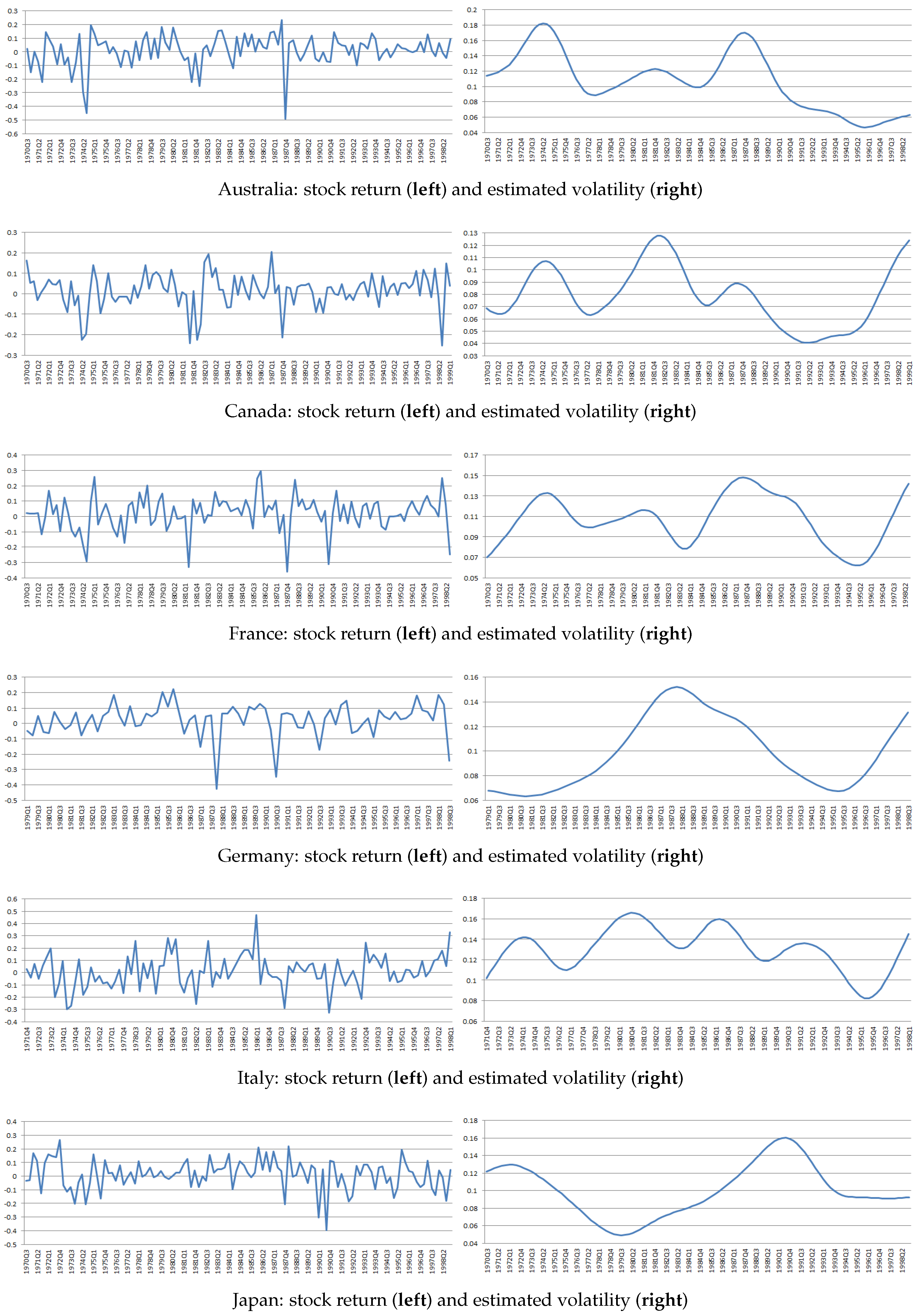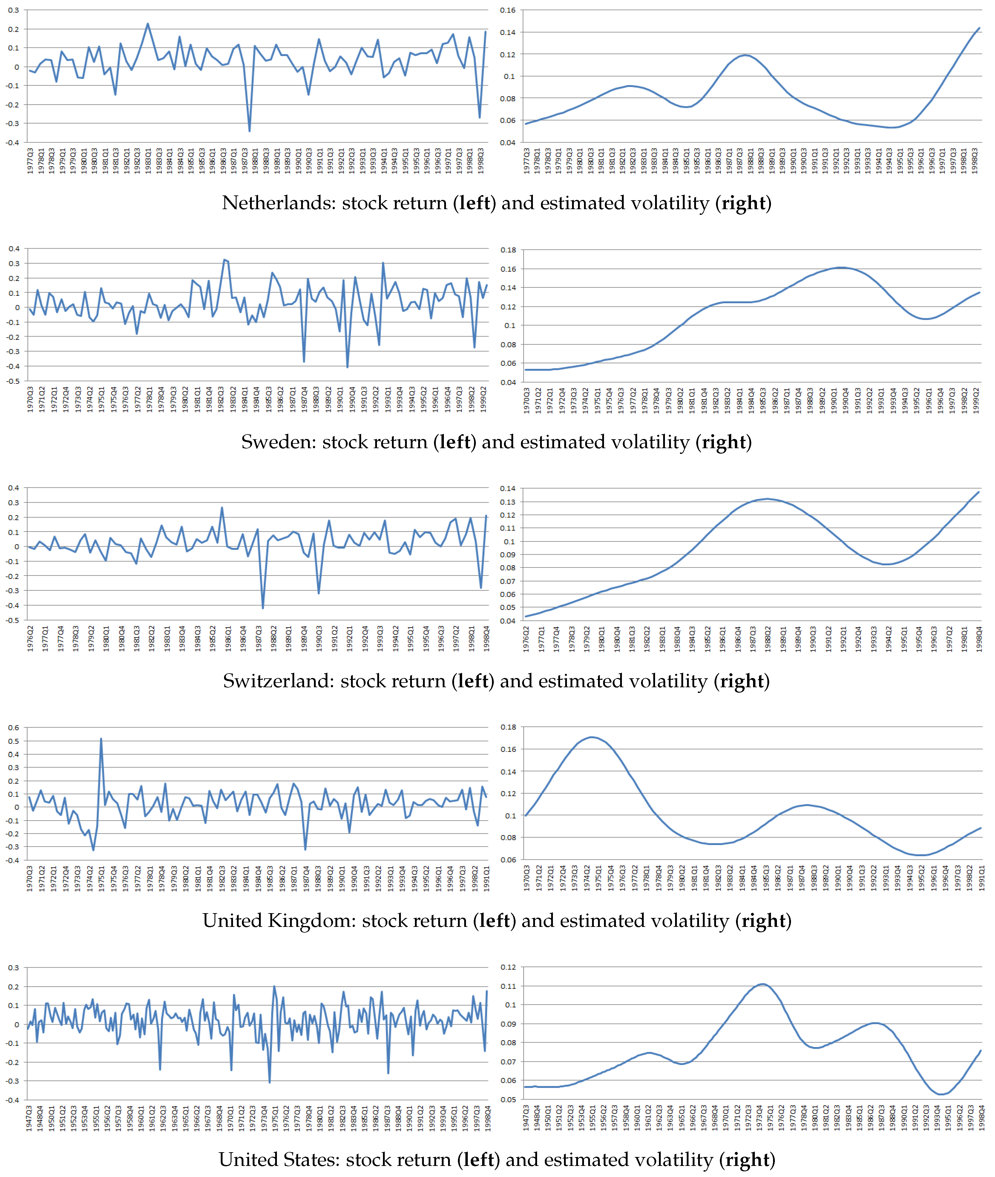The bandwidths $b_{ij}\left(T\right)$ were selected using leave-one-out cross-validation using each country-specific sample. The volatilities of returns exhibit significant time variation across countries, as shown in Figure 1 and Figure 2. This provides empirical support for the identifying assumption of time-varying volatility. Furthermore, we calculate the correlation between between $r_t$ and $v_t^{*}$ to check whether the multicollinearity is avoided. The last column in Table 1 reports the corresponding correlations between $r_t$ and $v_t^{*}$ for each country. The correlations are all substantially below unity, consistent with the theoretical argument that time-varying volatility restores identification.

Table 2. Confidence interval based on the control function approach and the weak-instrument robust tests.

Country	Sample Period	CF	AR	LM	CLR
AUL	1970.3–1998.4	[−0.11, 0.14]	[$-\infty$, ∞]	[$-\infty$, ∞]	[$-\infty$, ∞]
CAN	1970.3–1999.1	[0.03, 0.28]	[0.02, 4.03]	[0.05, 0.35]	[0.04, 0.41]
FR	1970.3–1998.3	[−0.03, 0.15]	[−0.28, 0.20]	[$-\infty$, ∞]	[−0.16, 0.11]
GER	1979.1–1998.3	[−0.01, 0.19]	[$-\infty$, ∞]	[$-\infty$, ∞]	[$-\infty$, ∞]
ITA	1971.4–1998.1	[−0.03, 0.17]	[$-\infty$, ∞]	[$-\infty$, ∞]	[$-\infty$, ∞]
JAP	1970.3–1998.4	[−0.05, 0.19]	[−0.05, 0.32]	[−1.01, 0.20]	[−0.02, 0.21]
NTH	1977.3–1998.4	[0.03, 0.19]	[$-\infty$, ∞]	[$-\infty$, ∞]	[$-\infty$, ∞]
SWD	1970.3–1999.2	[−0.01, 0.07]	[$-\infty$, ∞]	[$-\infty$, ∞]	[$-\infty$, ∞]
SWT	1976.2–1998.4	[−0.04, 0.21]	[$-\infty$, ∞]	[$-\infty$, ∞]	[$-\infty$, ∞]
UK	1970.3–1999.1	[0.02, 0.29]	[−0.51, −0.02]	[$-\infty$, ∞]	[$-\infty$, ∞]
USA	1947.3–1998.4	[0.11, 0.27]	[−0.21, −0.02]	[$-\infty$, ∞]	[$-\infty$, ∞]

Note: This table reports the confidence interval of EIS estimated by the proposed approach and the weak-instrument robust tests. CF refers to the proposed estimator. AR refers to the Anderson–Rubin test. LM refers to the Kleibergen-LM test. CLR refers to the Conditional Likelihood Ratio test.

reports confidence intervals for the EIS estimated using our control function method and compares them to intervals derived from three commonly used weak-instrument robust tests: the Anderson–Rubin [30], Kleibergen-LM [31], and Conditional Likelihood Ratio [32,33], as reported in [10]. In most cases, the confidence intervals obtained by three weak-instruments robust tests are extremely wide or unbounded, reflecting the limited power of conventional weak-IV methods. In contrast, our approach obtains narrower, informative intervals. The estimated EIS values are uniformly modest across countries, roughly in the −0.05 to 0.3 range, indicating a limited willingness of households to shift consumption over time. In economic terms, an EIS of this magnitude implies a strong preference for consumption smoothing. These findings are aligned with prior empirical findings that the EIS is typically low (e.g., [7,28]), standing in contrast to the much larger values (EIS well above 1) required by certain asset-pricing frameworks like long-run risk models [8]. Moreover, our approach delivers considerably tighter confidence intervals than standard weak-IV methods, reflecting a substantial gain in identification power. The improved precision suggests that by exploiting time-varying volatility, we can estimate the EIS with much greater confidence. These results demonstrate the empirical relevance of the theoretical framework developed in earlier sections.

5. Concluding Remarks

This paper develops a feasible control function approach for identifying and estimating linear models with endogenous regressors without valid instruments. The method exploits time-varying volatility in the reduced-form errors as a source of identification, offering an alternative when conventional instrumental variable techniques are infeasible or unreliable.

The main contribution lies in demonstrating that conditional heteroskedasticity can restore identification even when valid instrumental variables are unavailable. By projecting the structural error term onto the reduced-form error terms and standardizing by the time-varying variance, the proposed estimator isolates exogenous variation that would otherwise be obscured by collinearity. Unlike approaches that rely on strong instruments, known heteroskedastic regimes [3], or parametric volatility models [4,5,6], our framework allows for smooth, nonparametric variation in second moments and does not require external exclusion restrictions.

We formally establish that the estimator is $\sqrt{T}$-consistent and asymptotically normal. Importantly, we show that the estimator remains valid under weak identification and heteroskedasticity, provided the volatility process satisfies mild regularity conditions. We also derive a test for endogeneity that does not require valid instruments, extending the logic of the Hausman–Wu test to settings where standard IV methods fail.

In an empirical application, we estimate the EIS using quarterly stock return and consumption data from eleven developed countries. The data exhibit substantial time variation in return volatility, consistent with the identifying assumptions. The proposed method produces confidence intervals that are narrower and more stable than those derived from conventional weak-instrument robust procedures, while remaining consistent with existing findings in the literature.

The results demonstrate both the empirical relevance and practical applicability of using heteroskedasticity as a source of identification. The approach provides a flexible alternative to instrument-based methods in settings where external instruments are weak, contested, or unavailable. More broadly, this framework suggests that structured time variation in second moments can offer credible identification strategies in a range of economic applications.