Testing the Temperature-Mortality Nonparametric Function Change with an Application to Chicago Mortality

Abstract

The relationship between temperature and mortality is well-documented, yet most existing studies assume this relationship remains static over time. This study investigates whether the temperature-mortality association in Chicago from 1987 to 2000 has changed in shape or location of key features, such as change points. We apply nonparametric regression techniques to estimate the temperature-mortality functions for each year using daily mortality and temperature data from the National Morbidity, Mortality, and Air Pollution Study (NMMAPS) database. A permutation-based test is used to assess whether the shapes of these functions differ across time, while a bootstrap procedure evaluates the consistency of change points. Intensive simulation studies are conducted to evaluate the permutation-based test and bootstrap procedure based on Type I error and power. The proposed tests are compared with F tests in terms of Type I error and power. For the real data set, the analysis finds significant variation in the functional shapes across years, indicating evolving mortality responses to temperature. However, the estimated change points—temperatures associated with peak mortality—remain statistically consistent. These findings suggest that while the population’s overall vulnerability pattern may shift, the temperature threshold linked to maximum mortality has remained stable. This study contributes to understanding the temporal dynamics of climate-sensitive health outcomes and highlights the importance of flexible modeling in public health and climate adaptation planning.

1. Introduction

The relationship between temperature and mortality has been widely studied in epidemiology, with numerous studies emphasizing the critical impacts of extreme temperatures on human health [1,2,3,4]. Both high and low temperatures have been linked to increased mortality, with vulnerable populations such as the elderly, young children, and individuals with preexisting health conditions being disproportionately affected [5]. Despite this robust body of research, much of it assumes a static relationship over time, overlooking the potential for temporal variations due to changes in environmental conditions, population characteristics, and adaptive responses. This static assumption could obscure evolving vulnerabilities or resilience within populations, particularly in the context of climate change.

Regression analysis plays a vital role in statistical modeling, particularly in understanding the influence of explanatory variables on a response variable. Nonparametric regression, which does not assume a predefined functional form, allows for flexible modeling of complex relationships. This study focuses on estimating and making inferences about the nonparametric function that describes the relationship between temperature and mortality, specifically analyzing whether the mortality-temperature functions remain consistent over time and whether they share common change points in their structure.

The articles studied the relationship between temperature and mortality, particularly in the context of climate change and extreme weather events, found that the relationship takes the form of a U-shaped or J-shaped association, where mortality rates rise at both low and high temperatures [6,7,8]. Research by [9,10] has shown that both heatwaves and cold spells significantly increase mortality, with the elderly and individuals with preexisting health conditions being particularly vulnerable. Similarly, ref. [11] found a strong correlation between high temperatures and mortality in London, particularly from cardiovascular and respiratory diseases. These findings underscore the public health risks posed by temperature extremes.

Despite this extensive research, most studies assume a static relationship between temperature and mortality, overlooking potential temporal variations. As climate change progresses, factors such as environmental shifts, population dynamics, and adaptive responses may alter the mortality-temperature relationship. The increasing frequency and intensity of extreme weather events, compounded by urban heat islands and demographic transitions, further complicate this association. Studies such as those by [1,4] highlight that both high-temperature variability and extreme temperatures contribute to mortality risk. Still, few studies rigorously examine whether this relationship evolves or changes over time.

Existing research often focuses on short-term studies or specific geographic regions, leaving gaps in understanding the long-term evolution of temperature-related mortality. Addressing these gaps is critical, particularly for developing countries and areas with limited healthcare infrastructure. Studies such as those by [12] project substantial increases in temperature-related mortality, particularly in vulnerable regions. Without significant mitigation and adaptation measures, the global burden of temperature-related mortality is expected to rise, as highlighted by [13].

Examining the stability of the temperature-mortality relationship is crucial for several reasons. First, it can indicate whether populations are becoming more resilient or more vulnerable to temperature extremes, providing critical insights for public health planning. Second, identifying temporal variations may help pinpoint factors driving these changes, such as improvements in adaptive capacity or increased exposure due to urbanization. Lastly, understanding these dynamics can enhance predictive modeling for future mortality trends under various climate scenarios.

The methodology employed in this study focuses on advanced statistical modeling techniques, including semiparametric methods, to assess whether the temperature-mortality functions have remained consistent over the years 1987–2000 for Chicago City, USA. By leveraging local linear polynomial kernel smoothing, the study aims to detect nonlinear and nonstationary patterns, enabling a more nuanced understanding of how temperature impacts mortality over time. Additionally, a test will be proposed and applied to Chicago data to determine if there is a significant change over time in the temperature-mortality relationship. Another test will examine whether the change points in the mortality-temperature nonparametric function are consistent over time.

This study contributes to the growing field of environmental epidemiology by systematically evaluating how the temperature-mortality relationship changes over time. The findings will offer actionable insights for climate adaptation, public health strategies, and mortality risk mitigation. Given the projected rise in extreme temperature events due to climate change, there is an urgent need for coordinated global efforts to understand and reduce temperature-related mortality. Future research should continue exploring regional vulnerabilities and developing targeted interventions to protect public health in an era of increasing climate instability.

The remainder of this paper is organized as follows. In Section 2, the nonparametric temperature-mortality function estimation is introduced. In Section 3, the procedure for testing the equality of the nonparametric function over the years is displayed. Intensive simulation studies are conducted in Section 4 to evaluate the proposed approaches and compare them to the traditional F test. The real data application is analyzed in Section 5. Section 6 includes a discussion, conclusion, and future research.

2. Functional Change Estimation and Inference

In this section, we develop the methodology used to estimate and analyze the temperature-mortality relationship using nonparametric regression models. We first introduce the modeling framework and define the concept of functional change and change points in Section 2.1. This includes the formulation of the group-specific nonparametric model and the interpretation of the change point as the temperature associated with peak mortality. In Section 2.2, we describe in detail the estimation procedure based on local polynomial kernel smoothing. This involves estimating the overall function and group-level deviations, enforcing identifiability constraints, and computing the estimated change points from the smoothed curves. These steps provide the foundation for the inference procedures discussed in Section 3.

2.1. The Nonparametric Function and Change Points

Let y be the vector of the response variable and x be the explanatory variable. The relationship between the two variables can be modeled using the following nonparametric regression model:

$$\mathbf{y}=f\left(\mathbf{x}\right)+\mathit{ϵ},$$

(1)

where f represents an unknown nonparametric smooth function and $\mathit{ϵ}$ is the error term with a mean equal to zero and variance ${\sigma }^2$. The main advantage of this model is its flexibility and ease of interpretation [14]. While our estimation approach follows the local polynomial framework discussed in [14], our contribution lies in developing accompanying inference procedures for testing the equality of nonparametric functions and their change points across groups.

Assume we have a categorical variable that has L number of levels or groups, and observed data are $(y_{ij},x_{ij}):i=1,\dots ,L;j=1,\dots ,n_j$, where $y_{ij}$ is the response of the i-th individual of the j-th group. The regression model can be written as follows:

$${\mathbf{y}}_{ij}=f_0\left(\mathbf{x}\right)+f_{ij}\left(\mathbf{x}\right)+{\mathit{ϵ}}_{ij},i=1,2,\dots ,L,j=1,2,\dots ,n_j.$$

(2)

For each level or group, the model (2) can be rewritten as follows:

$${\mathbf{y}}_i=f_0\left(\mathbf{x}\right)+f_i\left(\mathbf{x}\right)+{\mathit{ϵ}}_i,i=1,\dots ,L,$$

(3)

where ${\mathit{ϵ}}_1,\dots ,{\mathit{ϵ}}_I$ are zero-mean errors, each corresponding to a level of i of the factor, and $f_0(·)$ represents the overall effect of x on y. The specific effect for the level i is given by $f_i\left(x\right)$. The mean regression curves are defined as follows:

$$w_i\left(\mathbf{x}\right)=f_0\left(\mathbf{x}\right)+f_i\left(\mathbf{x}\right),i=1,\dots ,L.$$

(4)

To ensure the model identifiability, the condition ${\sum }_{i=1}^L{f}_i\left(\mathbf{x}\right)=0$ is imposed for all $\mathbf{x}$.

Suppose that it is found that the nonparametric functions for all possible levels of i ($i=1,\dots ,L$) are not equal. In that case, a follow-up analysis should be performed to determine whether the nonparametric functions have the same change points. The change point ${\theta }_i$ for level i is defined as follows:

$${\theta }_i=arg\underset{\mathbf{x}}{min}{f}_i\left(\mathbf{x}\right).$$

(5)

The change point represents the temperature at which mortality reaches its minimum. Mortality decreases as temperature approaches this point from below and increases as temperature moves beyond it. Therefore, this change point corresponds to the optimal temperature for human health, as it marks the level associated with the lowest mortality risk.

2.2. The Nonparametric Function Estimation

To estimate the factor-by-curve regression function in (2), we use local linear polynomial kernel smoothers [15,16,17]. Given a sample of n independent and identically distributed (i.i.d.) observations, considering data across all levels of a factor J, the estimator for $f_0(·)$ at a point x is given by ${\widehat{f}}_0\left(x\right)={\widehat{\beta }}_0\left(x\right)$. Here, ${\widehat{\beta }}_0\left(x\right)$ is the first component of the vector $({\widehat{\beta }}_0\left(x\right),{\widehat{\beta }}_1\left(x\right),\dots ,{\widehat{\beta }}_p\left(x\right))$, which minimizes the following expression:

$$\sum _{k=1}^n{\left[y_k-\sum _{j=0}^p{\beta }_j\left(x\right){(x_k-x)}^j\right]}^2\xi \left({\displaystyle \frac{x_k-x}{h_0}}\right),$$

where $\xi$ is a kernel function (the Gaussian function is commonly used), $h_0$ is the bandwidth or smoothing parameter, and p is the degree of polynomiality.

After estimating $f_0(·)$, the estimator for $f_i(·)$ at point x is obtained as ${\widehat{f}}_i\left(x\right)={\widehat{\beta }}_{0i}\left(x\right)$ for each level i, $i=1,\dots ,L$. Here, ${\widehat{\beta }}_{0i}\left(x\right)$ is the first component of the vector $({\widehat{\beta }}_{0i}\left(x\right),{\widehat{\beta }}_{1i}\left(x\right),\dots ,{\widehat{\beta }}_{pi}\left(x\right))$, which minimizes the following:

$$\sum _{k=1}^n{\left[y_k^{*}-\sum _{j=0}^p{\beta }_{ji}\left(x\right){(x_k-x)}^j\right]}^2\xi \left({\displaystyle \frac{x_k-x}{h_i}}\right)I\{J_k=i\},$$

where $y_k^{*}=y_k-{\widehat{f}}_0\left(x_k\right)$, $h_i$ is the bandwidth to estimate $f_i(·)$, and J is the indicator function.

To ensure that the identifiability condition is satisfied, the following adjustment is made. For each x, calculate the mean of the specific effects of each level $S\left(x\right)={\sum }_{i=1}^L{\widehat{f}}_i\left(x\right)/L$ and replace the original ${\widehat{f}}_i\left(x\right)$ by ${\widehat{f}}_i\left(x\right)-S\left(x\right)$ and ${\widehat{f}}_0\left(x\right)$ by ${\widehat{f}}_0\left(x\right)+S\left(x\right)$. The estimated curve for each level, at point x, is given by ${\widehat{w}}_i\left(x\right)={\widehat{f}}_0\left(x\right)+{\widehat{f}}_i\left(x\right)$ for $i=1,\dots ,L$.

A natural estimate for the change point, ${\theta }_i$, is obtained as the value that maximizes the following:

$${\widehat{w}}_i\left(k_1\right),\dots ,{\widehat{w}}_i\left(k_G\right),$$

where $k_1,\dots ,k_G$ are grid points spaced evenly over the range of x, and $K_G$ is the number of equally spaced selected points in the range x. It is important to note that this estimation approach is appropriate when the support of x is consistent across all levels and is confined within a closed and bounded interval. It is important to note that the consistency of the estimators ${\widehat{f}}_i(·)$ requires that the number of observations within each group $n_j\to \infty$ as the total sample size increases. Under standard regularity conditions on the kernel function and bandwidth selection, local linear kernel smoothing estimators are known to be consistent (see [15]).

3. Inference Procedures

The test statistic $T\left(y\right)$ is designed to compare the goodness-of-fit between the null and alternative models by quantifying the ratio of the residual sums of squares. Under the null hypothesis, all group-specific functions are equal, and residuals from the reduced model should be comparable to those from the full model. If the null is false, the alternative model should result in a noticeably smaller residual sum of squares. Thus, a large value of $T\left(y\right)$ provides evidence against the null. To assess the significance of the observed test statistic $T\left(y\right)$, we use a permutation procedure. This approach is justified under the assumption that residuals are exchangeable under the null hypothesis. By permuting residuals and recalculating $T\left(y\right)$ for each permutation, we approximate the null distribution of the test statistic and compute an empirical p-value as the proportion of permuted statistics that are more extreme than the observed one. This method avoids reliance on asymptotic approximations and provides a robust nonparametric inference tool.

3.1. Testing the Equality of the Nonparametric Functions

The null and alternative hypotheses take the following form:

$$H_0:f_1(·)=\dots =f_L(·)=0$$

$$H_a:\mathrm{at}\mathrm{least}\mathrm{one}\mathrm{of}\mathrm{the}\mathrm{nonparametric}\mathrm{functions},f_i(·),\mathrm{is}\mathrm{not}\mathrm{equal}\mathrm{to}0.$$

When the null hypothesis, $H_0$ is true, the model (2) takes the form $\mathbf{y}=f\left(\mathbf{x}\right)+\mathit{ϵ}$, for all the factor levels, and residuals under the null hypothesis can be calculated as ${\widehat{\mathit{ϵ}}}^{\left(0\right)}=\mathbf{y}-\widehat{f}{\left(\mathbf{x}\right)}^{\left(0\right)}$, where ${\widehat{\mathit{ϵ}}}^{\left(0\right)}$ is the estimated error under the null hypothesis, and $\widehat{f}{\left(\mathbf{x}\right)}^{\left(0\right)}$ is the estimated nonparametric function under the null hypothesis. When the hull hypothesis is true, the residuals are assumed to be exchangeable. Under the alternative hypothesis, one can calculate the residuals as ${\widehat{\mathit{ϵ}}}^{\left(1\right)}=\mathbf{y}-\widehat{f}{\left(\mathbf{x}\right)}^{\left(1\right)}$, where ${\widehat{\mathit{ϵ}}}^{\left(1\right)}$ is the estimated error under the alternative hypothesis, and $\widehat{f}{\left(\mathbf{x}\right)}^{\left(1\right)}$ is the estimated nonparametric function under the alternative hypothesis. Then the test statistic is calculated as follows:

$$T\left(\mathbf{y}\right)={\displaystyle \frac{{\left[{\widehat{\mathit{ϵ}}}^{\left(0\right)}\right]}^T\left[{\widehat{\mathit{ϵ}}}^{\left(0\right)}\right]}{{\left[{\widehat{\mathit{ϵ}}}^{\left(1\right)}\right]}^T\left[{\widehat{\mathit{ϵ}}}^{\left(1\right)}\right]}},$$

where $T\left(\mathbf{y}\right)$ is the test statistic value computed using the dataset $\mathbf{y}$. The distribution of the test statistic, T, is approximated by the following permutation-based procedure and used to make a decision about testing the equality of the nonparametric functions, or whether there is a functional change:

• Step 1: Fit the model under the null hypothesis and obtain the vector of residuals, ${\widehat{\mathit{ϵ}}}^{\left(0\right)}$ that minimizes ${\sum }_{k=1}^n(y_k-\widehat{f}(x_k{{)}^{(0)})}^2$. Fit the model under the alternative hypothesis and obtain the vector of residuals, ${\widehat{\mathit{ϵ}}}^{\left(1\right)}$, that minimizes ${\sum }_{k=1}^n(y_k-\widehat{f}(x_k{{)}^{(1)})}^2$.
• Step 2: Calculate the test statistic $T_{\mathbf{y}\left(\mathbf{0}\right)}={\displaystyle \frac{{\left[{\widehat{\mathit{ϵ}}}_{\mathbf{y}\left(0\right)}^{\left(0\right)}\right]}^T\left[{\widehat{\mathit{ϵ}}}_{\mathbf{y}\left(0\right)}^{\left(0\right)}\right]}{{\left[{\widehat{\mathit{ϵ}}}_{\mathbf{y}\left(0\right)}^{\left(1\right)}\right]}^T\left[{\widehat{\mathit{ϵ}}}_{\mathbf{y}\left(0\right)}^{\left(1\right)}\right]}},$ where ${\mathbf{y}}_{\left(0\right)}$ denotes the original dataset and ${\widehat{\mathit{ϵ}}}_{{\mathbf{y}}_{\left(0\right)}}^{\left(0\right)}$ and ${\widehat{\mathit{ϵ}}}_{{\mathbf{y}}_{\left(0\right)}}^{\left(1\right)}$ are the residuals under the null and alternative hypotheses of the original dataset, respectively;
• Step 3: Since the errors are exchangeable by assumption and we need to estimate the unknown distribution of T, we permute the residuals, ${\widehat{\mathit{ϵ}}}^{\left(0\right)}$, and add them back to the null modeled means, ${\mathbf{y}}_{\left(m\right)}=\widehat{f}{\left(\mathbf{x}\right)}^{\left(0\right)}+{\widehat{\mathit{ϵ}}}_m^{\left(0\right)}$, where m represents the $m^{th}$ permutation, ${\widehat{\mathit{ϵ}}}_m^{\left(0\right)}$ is the permuted $n\times 1$ vector of residuals and ${\mathbf{y}}_{\left(m\right)}$ is $n\times 1$ vector of permuted responses;
• Step 4: For the permuted dataset, ${\mathbf{y}}_{\left(m\right)}$, fit the null and alternative hypotheses the same way as in step 1 and compute the test statistic $T_{\mathbf{y}\left(\mathbf{m}\right)}={\displaystyle \frac{{\left[{\widehat{\mathit{ϵ}}}_{\mathbf{y}\left(m\right)}^{\left(0\right)}\right]}^T\left[{\widehat{\mathit{ϵ}}}_{\mathbf{y}\left(m\right)}^{\left(0\right)}\right]}{{\left[{\widehat{\mathit{ϵ}}}_{\mathbf{y}\left(m\right)}^{\left(1\right)}\right]}^T\left[{\widehat{\mathit{ϵ}}}_{\mathbf{y}\left(m\right)}^{\left(1\right)}\right]}},$ where, ${\widehat{\mathit{ϵ}}}_{{\mathbf{y}}_{\left(m\right)}}^{\left(0\right)}$ and ${\widehat{\mathit{ϵ}}}_{{\mathbf{y}}_{\left(m\right)}}^{\left(1\right)}$ are the residuals from fitting the ${\mathit{m}}^{\mathit{th}}$ permuted dataset under the null and alternative hypotheses, respectively;
• Step 5: Repeat Step 3 and Step 4 for a large number, say $M=10,000$, and combine the values of $T_{\mathbf{y}\left(\mathbf{m}\right)},m=1,2,\dots ,M$, and the value of the original dataset, $T_{\mathbf{y}\left(\mathbf{0}\right)}$, and then calculate the empirical p-value as

  $$p\text{-}\mathrm{value}={\displaystyle \frac{\mathrm{Number}\mathrm{of}\mathrm{times}\mathrm{that}[T_{\mathbf{y}\left(\mathbf{m}\right)}\ge T_{\mathbf{y}\left(\mathbf{0}\right)}]}{M+1}},m=0,1,\dots ,M,$$

  which measures how extreme the $T_{\mathbf{y}\left(\mathbf{0}\right)}$ value is.

Finally, the decision rule consists of rejecting the null hypothesis if the empirical p-value is less than the significance level $\alpha$.

3.2. Testing the Equality of the Change Points of the Nonparametric Functions

If the null hypothesis is rejected, a follow-up test is required to find whether the nonparametric functions have the same change points in the temperature-mortality relationship. The following are the null and the alternative hypotheses for testing equal change points for the nonparametric functions.

$$H_0:{\theta }_1=\cdots ={\theta }_L$$

$$H_1:\mathrm{At} \mathrm{least} \mathrm{one} \mathrm{nonparametric} \mathrm{function} \mathrm{has} \mathrm{a} \mathrm{different} \mathrm{change} \mathrm{point},$$

where ${\theta }_i,(i=1,2,\dots ,L)$, is the temperature that is associated with the highest mortality. To test the null hypothesis versus the alternative, one can use a bootstrap procedure to obtain the 95% simultaneous bootstrap confidence intervals for the difference between each pair of change points, ${\theta }_i-{\theta }_j$.

Suppose we estimate p simultaneous confidence intervals of ${\widehat{\theta }}_i-{\widehat{\theta }}_j$. The Bonferroni-adjusted bootstrap confidence interval for each simultaneous confidence interval of ${\widehat{\theta }}_i-{\widehat{\theta }}_j$ is given by the following:

$${\mathrm{CI}}_{i-j}=[({\widehat{\theta }}_i-{\widehat{\theta }}_j)-z_{1-{\displaystyle \frac{\alpha }{2p}}}·\widehat{\sigma },({\widehat{\theta }}_i-{\widehat{\theta }}_j)+z_{1-{\displaystyle \frac{\alpha }{2p}}}·\widehat{\sigma }],\mathrm{for}i,j=1,\dots ,L,i\ne j,$$

where L is the number of groups or levels, $\widehat{\sigma }$ is the bootstrap estimate of the standard error of ${\widehat{\theta }}_i-{\widehat{\theta }}_j$, and $z_{1-{\displaystyle \frac{\alpha }{2p}}}$ is the $(1-{\displaystyle \frac{\alpha }{2p}})$ quantile of the standard normal distribution. The Bonferroni adjustment is used to ensure that the family-wise error rate is controlled at level $\alpha$ using the Bonferroni correction.

If the simultaneous bootstrap confidence interval contains zero, one can declare that the two nonparametric functions have equal change points; otherwise, the two nonparametric functions have unequal change points.

4. Simulation Studies

In this section, simulation studies were conducted to evaluate the finite-sample performance of the proposed permutation-based test to detect functional changes and the bootstrap-based test to compare change points among groups. The empirical Type I error and power under different scenarios were used, considering varying sample sizes and noise levels.

4.1. Simulation Settings

Let the number of groups be equal to 3, $L=3$, with balanced sample sizes $n_i\in \{50,100,200\}$ and noise levels $\sigma \in \{1,2,3\}$. The model described in Equation (2) takes the following form:

$$y_{ij}=f_0\left(x_{ij}\right)+f_i\left(x_{ij}\right)+{\mathit{ϵ}}_{ij},i=1,2,3;j=1,\dots ,n_i,(n_i=50,100,200),$$

where $x_{ij}\sim \mathrm{Uniform}(0,40)$, ${\mathit{ϵ}}_{ij}\sim \mathcal{N}(0,{\sigma }^2)$, $f_0\left(x\right)=0.02{(x-20)}^2$ is the overall function, $f_i\left(x\right)$ varies between scenarios to simulate differences across groups.

• Simulation setting 1 (Null: No Functional difference): $f_i\left(x\right)=0$ for all i. In this simulation, it is assumed that all the groups have the same regression function $f_0\left(x\right)$. This simulation is used to evaluate the permutation test in terms of Type I error.
• Simulation setting 2 (Alternative: Different Shapes):

  $$\begin{array}{cc}\hfill f_1\left(x\right)& =0,\hfill \\ \hfill f_2\left(x\right)& =0.01{(x-25)}^2,\hfill \\ \hfill f_3\left(x\right)& =0.02{(x-15)}^2.\hfill \end{array}$$
  In this simulation, it is assumed that the groups have different regression functions. The datasets were simulated under this setting, and then the permutation test detects how many times the change function is detected, and then the power is calculated.
• Simulation setting 3 (Alternative: Different Change Points):

  $$f_i\left(x\right)=-0.02{(x-{\theta }_i)}^2+c_i,\theta =(20,22,24),$$

  where $c_i$ are constants chosen so that all functions have similar average levels. This simulation is used to evaluate the bootstrap-based test in which the bootstrapped simultaneous confidence intervals are calculated and find whether the change points are equal at a significance level $\alpha$.

Each simulation setting was replicated 10,000 times to compute the empirical Type I error and power. Figure 1 displays one of the 10,000 simulated data under each setting.

4.2. Simulation Results

The results of the three simulation settings are displayed in

Table 1. Simulation setting 1: empirical Type I error under null hypothesis using the permutation test.

Noise Level ($\mathit{\sigma }$)	Sample Size ($\mathit{n}=50$)	Sample Size ($\mathit{n}=100$)	Sample Size ($\mathit{n}=200$)
Low ($\sigma =1$)	0.048	0.050	0.051
Medium ($\sigma =2$)	0.054	0.049	0.047
High ($\sigma =3$)	0.058	0.051	0.050

Note: This table evaluates the empirical Type I error rates under the null hypothesis of no functional difference across groups using the permutation test over 10,000 simulations.

,

Table 2. Simulation setting 2: power to detect functional shape differences using the permutation test.

Noise Level ($\mathit{\sigma }$)	Sample Size ($\mathit{n}=50$)	Sample Size ($\mathit{n}=100$)	Sample Size ($\mathit{n}=200$)
Low ($\sigma =1$)	0.86	0.94	0.99
Medium ($\sigma =2$)	0.84	0.92	0.96
High ($\sigma =3$)	0.82	0.89	0.95

Note: This table shows the empirical power of the permutation test to detect differences in functional shapes across groups under Setting 2 over 10,000 simulations.

and

Table 3. Simulation setting 3: power to detect change point differences using the bootstrap test.

Noise Level ($\mathit{\sigma }$)	Sample Size ($\mathit{n}=50$)	Sample Size ($\mathit{n}=100$)	Sample Size ($\mathit{n}=200$)
Low ($\sigma =1$)	0.88	0.97	0.98
Medium ($\sigma =2$)	0.84	0.95	0.96
High ($\sigma =3$)	0.85	0.93	0.94

Note: This table displays the empirical power of the bootstrap test for detecting differences in change points across groups under Setting 3 over 10,000 simulations.

. Table 1 shows Type I error empirical values under different sample sizes and standard deviation values. One can see that the empirical Type I error values are close to the nominal values.

Table 2 shows the power values for different sample sizes and the standard deviation values to detect the change in the regression functions. The power values of the permutation test increase as the sample size increases.

Table 3 reveals the power for the change point difference in regression functions. One can see that the power is high, especially for large samples. In sum, the results show that both the permutation-based and bootstrap-based tests maintain nominal Type I error rates and have strong power properties, particularly with larger sample sizes and lower noise levels. These findings validate the proposed methods for detecting nonparametric functional changes and evaluating the stability of change points across groups.

4.3. Comparison Results

This subsection includes a simulation study to compare our proposed permutation and bootstrap approaches with traditional F tests.

Table 4. Comparison of Type I error and power: proposed methods (permutation and bootstrap) vs. F-Test.

Setting	Method	Metric	Sample Size ($\mathit{n}=100$)	Sample Size ($\mathit{n}=200$)
	Permutation	Type I Error	0.049	0.047
Setting 1	F-Test	Type I Error	0.070	0.065
	Permutation	Power	0.92	0.96
Setting 2	F-Test	Power	0.78	0.85
	Bootstrap	Power (CP diff.)	0.95	0.96
Setting 3	F-Test	Power (CP diff.)	0.61	0.70

Note: Results are based on 10,000 replications for each setting. Type I Error is measured under the null hypothesis; Power is measured under the specified alternative. Setting 1: No functional difference. Setting 2: Different function shapes across groups. Setting 3: Same shape but different change points (CPs).

shows that the proposed bootstrap and permutation tests outperform the traditional functional F test in all scenarios evaluated. In Setting 1 (no functional difference), the permutation test maintains empirical Type I error rates close to the nominal level (approximately 5%), while the F test tends to inflate Type I error, particularly in smaller sample sizes. In Setting 2, where group-specific functional shapes differ, the permutation test exhibits substantially higher power than the F-test, especially for moderate to large sample sizes. For Setting 3, where the change points vary but the overall functional shapes remain similar, the bootstrap-based test shows markedly superior power compared with the F-test, which lacks sensitivity to subtle shifts in the change point location. These findings highlight the robustness and effectiveness of the proposed methods in detecting both structural changes in the functional form and temporal shifts in critical temperature thresholds.

5. Real Application

In the National Morbidity, Mortality, and Air Pollution Study (NMMAPS), daily data were collected from 1 January 1987 to 31 December 2000 across 108 U.S. cities to investigate the effects of air pollution on health in the United States [18]. The dataset includes numerous variables, such as temperature, deaths, nitrogen dioxide, relative humidity, ozone, PM10, and others. Many articles studied these data, such as [19], in which the association between cardiovascular mortality and temperature has been investigated by estimating the nonparametric temperature-mortality function. However, no study has studied the relationship between temperature and mortality over the years to find whether the function curve changed over the years or whether the nonparametric functions have the same change points.

Daily mortality counts were sourced from the National Center for Health Statistics, while pollution data originated from the U.S. national air monitoring network, provided by the EPA Aerometric Information Retrieval System database. Weather data were obtained from the National Climatic Data Center. The dataset was publicly available from June 2004 until 2011, when it was removed due to privacy concerns. However, data from Chicago remain accessible through the R 4.2.1 package “dlnm” which was utilized in this study.

The study starts by exploring the Chicago mortality and temperature data before applying the tests introduced in Section 3.

Table 5. Numerical summary of mortality and temperature for the first and last three years.

Years	Variable	Min	1st Qu.	Median	Mean	3rd Qu.	Max
1987–1989	Temperature	−21.389	1.389	10.278	10.092	19.722	31.944
	Mortality	77.0	108.0	117.0	117.7	125.0	186.0
1998–2000	Temperature	−18.889	2.778	12.222	10.996	20.000	32.222
	Mortality	73.0	101.0	110.0	111.5	121.0	164.0

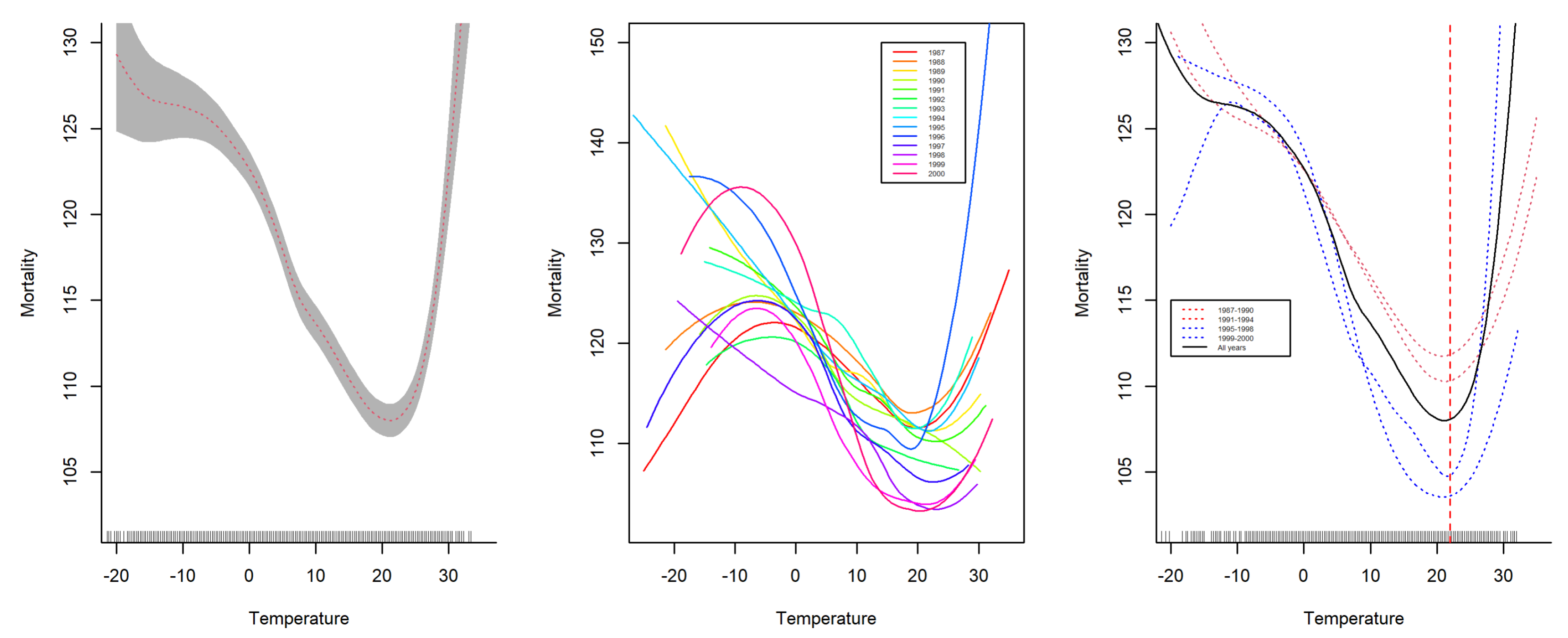
displays the numerical summary of temperature and mortality for the first three years (1987–1989) and the last three years (1998–2000). The table indicates that mortality decreased while temperature increased. Figure 2 (left) displays the smoothed nonparametric temperature-mortality function for all years combined, Figure 2 (middle) displays the smoothed nonparametric temperature-mortality function for each year, and Figure 2 (right) displays the smoothed function for each consecutive four-year period. The figure suggests that the function evolves, with higher years corresponding to a lower mortality function curve, particularly around the temperature change point of approximately 20 °C. 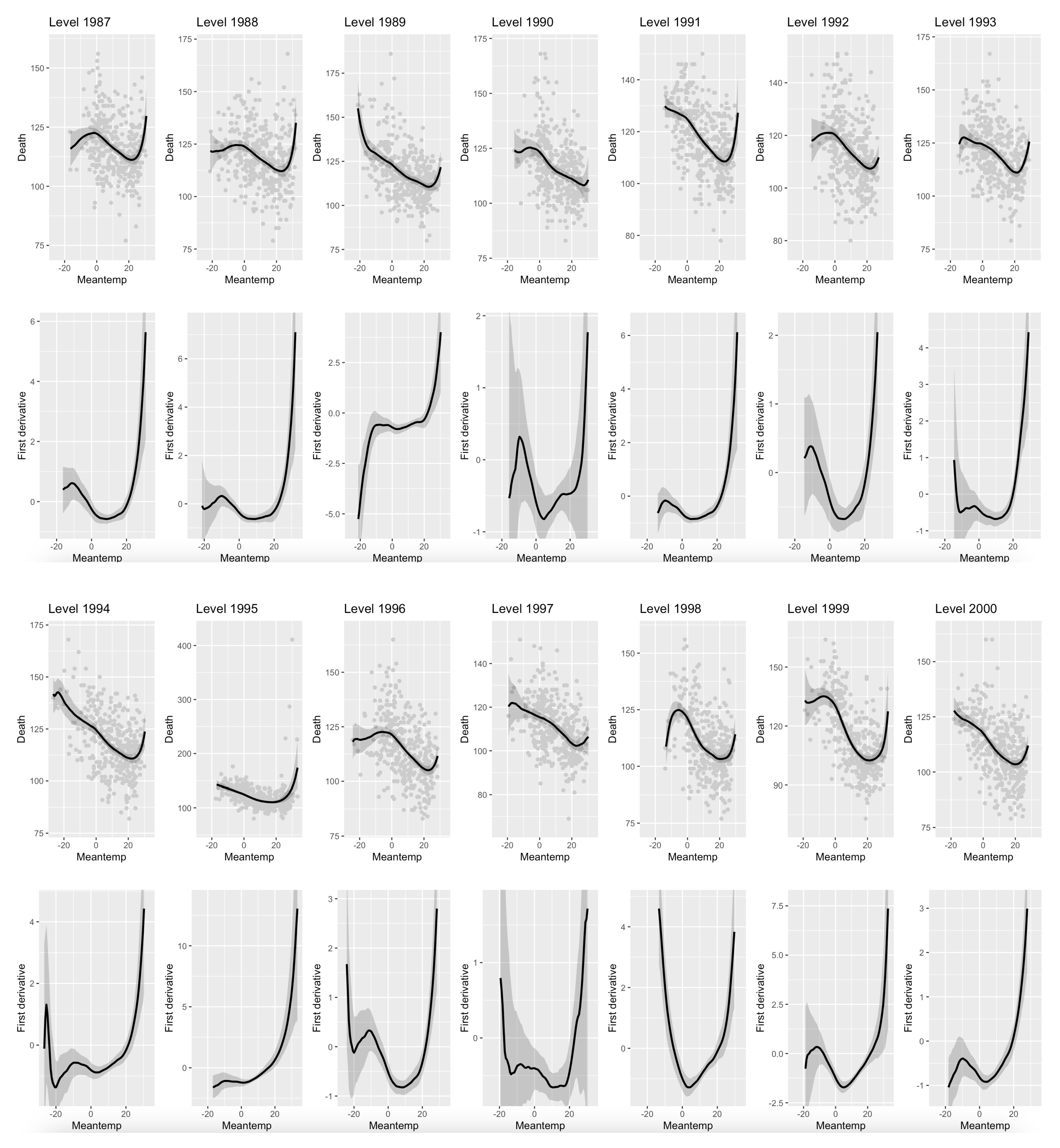Figure 3 displays the smoothed nonparametric temperature-mortality function for each of the 14 years and its first derivative along with the 95% confidence interval.

The test for equality of the nonparametric functions described in Section 3.1 and the test for equality of the change points in the mortality-temperature functions described in Section 3.2 are applied to the Chicago data.

Table 6. Change points of each year along with the 95% confidence interval (LL stands for the lower limit of the confidence interval and UL stands for the upper limit of the confidence interval) for the mortality-temperature nonparametric functions and its derivative.

	Nonparametric Function			Derivative Function
Year	Change Point	LL	UL	Change Point	LL	UL
1987	23.29 *	22.25	24.27	14.92 *	8.76	19.51
1988	22.34 *	20.65	23.70	11.31 *	5.40	15.44
1989	23.34 *	22.01	24.15	1.98	−4.97	21.80
1990	24.32 *	22.44	NA	-2.40	−4.97	21.58
1991	21.77 *	20.44	23.10	8.16 *	1.07	12.69
1992	21.29 *	18.84	NA	8.31	−4.97	13.97
1993	22.39 *	21.01	24.10	12.02 *	6.79	15.47
1994	21.67 *	19.39	23.60	2.55	−4.97	9.73
1995	17.01 *	13.49	21.24	−4.97 *	−4.97	−0.62
1996	22.01 *	20.63	23.79	9.59 *	3.22	13.09
1997	23.05 *	21.86	24.96	−4.97	−4.97	19.15
1998	21.25 *	19.70	22.86	1.84	−4.97	10.04
1999	21.96 *	18.58	24.86	6.17 *	4.26	8.73
2000	24.96 *	20.72	24.96	4.07	−4.97	24.68

* Means significant at 5% significance level. NA means calculated the UL is out of the temperature range of that year.

shows the change points of the mortality-temperature function for each year with the lower limit (LL) and the upper limit (UL) of the 95% confidence intervals. It also displays the change points in the derivative functions with lower and upper limits of the 95% confidence intervals. It reveals that all the change points in the nonparametric functions are significant because the lower and upper limits have positive signs. However, some of the change points in the derivative functions are not significant. 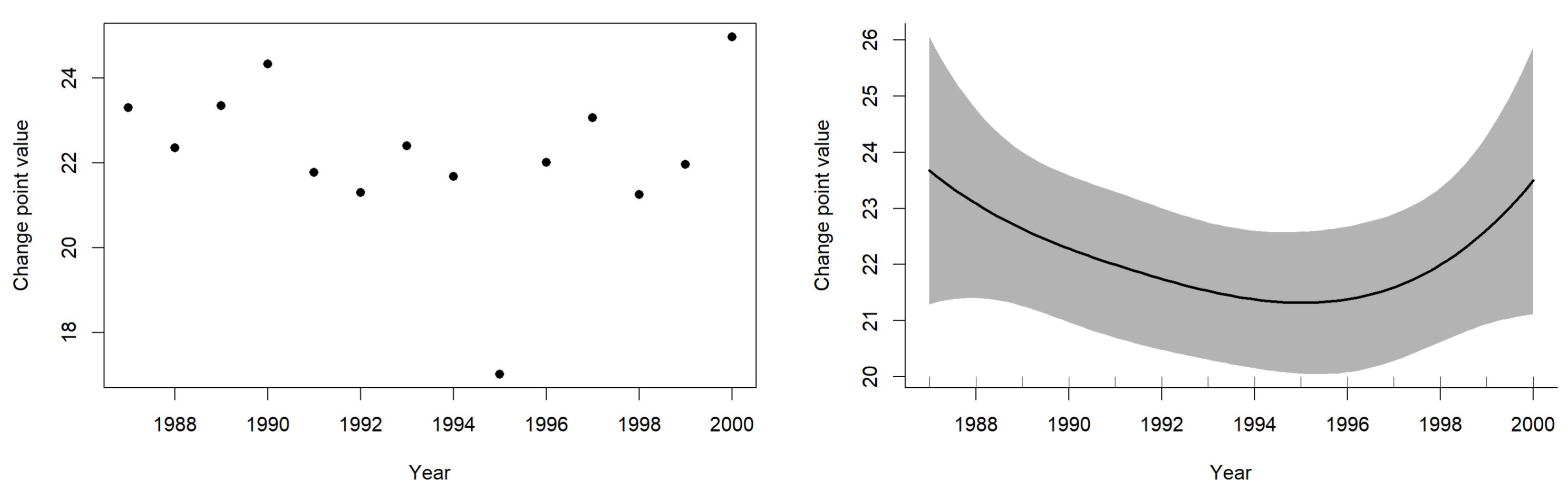Figure 4 (left) reveals that there is no trend in the change point values; there is no relationship between the year and the change point value, however, the smoothed faction displayed in Figure 4 (right) reveals that there is a pattern of decreasing change point value and then increasing; however, that is because of one change point of the year 1997 which is considered an outlier.

To find whether the mortality functions of all 14 years have the same shape, it is found that p-value < 0.001 for testing equal mortality-temperature nonparametric functions. As a result, the null hypothesis was rejected and it was concluded that the temperature-mortality functions do not have the same shapes at all 14 years at 5% significance level. As a follow-up analysis to see whether the change points in the mortality-temperature nonparametric functions for all 14 years have the same change point values, the test described in Section 3.2 was run. It is found that p-value = 0.048, which means that the functions do not have the same change points for all 14 years as displayed in Table 6. However, there is no pattern in the change point values over the years. The programs used in the paper are available upon request.

6. Conclusions and Future Research

In this article, an approach is presented to test the change in regression functions between groups or levels of a categorical variable, and to explore whether the change points are equal. An intensive simulation study was conducted to systematically evaluate the finite-sample performance of the proposed test procedures under various scenarios, such as different levels of noise, sample sizes, and functional shapes. Based on the empirical Type I error and power, it is found that the testing procedures are effective in detecting functional change and testing the equality of the change points. The proposed tests are compared with F tests and it was found that the proposed tests outperform the traditional functional F test in all scenarios evaluated.

Additionally, this study examined the temporal evolution of the temperature-mortality relationship in Chicago from 1987 to 2000 using nonparametric regression techniques. By applying local linear polynomial kernel smoothing and rigorous inference procedures, we found that the functional form of the temperature-mortality relationship significantly varies across years, indicating dynamic changes in population vulnerability or adaptation to temperature extremes. However, the analysis revealed that the change points, the temperatures at which mortality is highest, remain consistent over time, suggesting a stable threshold of critical risk despite structural changes in the overall relationship.

These findings underscore the importance of modeling strategies that accommodate temporal heterogeneity when assessing climate-sensitive health outcomes. Static models may overlook important variations that have implications for public health interventions and climate resilience planning.

Future research should extend this analysis to other geographic regions and periods to evaluate the generalizability of the observed patterns. Incorporating additional environmental and sociodemographic covariates, such as air pollution, urban heat island effects, and healthcare access, may further elucidate the mechanisms underlying the changing mortality response. Furthermore, developing methods that jointly model change in both the function shape and threshold behavior across space and time will be valuable for advancing epidemiological and environmental risk assessments in a changing climate. Simulation studies are conducted to evaluate the proposed tests; however, another direction for future research is theoretical work that could explore the asymptotic distribution and power properties of the proposed test statistics to formally establish their performance guarantees and limitations.

References

1. Gasparrini, A.; Guo, Y.; Hashizume, M.; Lavigne, E.; Zanobetti, A.; Schwartz, J.; Tobias, A.; Tong, S.; Rocklöv, J.; Forsberg, B.; et al. Mortality risk attributable to high and low ambient temperature: A multicountry observational study. Lancet 2015, 386, 369–375. [Google Scholar] [CrossRef] [PubMed]
2. Mahmoud, H.F.F. Semiparametric single index multi change points model with an application of environmental health study on mortality and temperature. Environmentics 2016, 27, 494–506. [Google Scholar] [CrossRef]
3. Mahmoud, H.F.F.; Kim, I. Semiparametric change points detection using single index spatial random effects model in environmental epidemiology study. PLoS ONE 2024, 19, e0315413. [Google Scholar] [CrossRef] [PubMed]
4. Guo, Y.; Gasparrini, A.; Armstrong, B.G.; Tawatsupa, B.; Tobias, A.; Lavigne, E.; Coelho, M.D.; Pan, X.; Kim, H.; Hashizume, M.; et al. Heat wave and mortality: A multicountry, multicommunity study. Environ. Health Perspect. 2018, 126, 087006. [Google Scholar] [CrossRef] [PubMed]
5. Huang, C.; Barnett, A.G.; Wang, X.; Tong, S. The impact of temperature on years of life lost in Brisbane, Australia. Nat. Clim. Change 2011, 2, 265–270. [Google Scholar] [CrossRef]
6. Armstrong, B. Models of the Relationship between ambient temperature and daily mortality. Epidemiology 2006, 17, 624–631. [Google Scholar] [CrossRef] [PubMed]
7. Chung, J.; Honda, Y.; Hong, Y.; Pan, X.; Guo, Y.; Kim, H. Ambient temperature and mortality: An international study in four capital cities East Asia. Sci. Total Environ. 2009, 408, 390–396. [Google Scholar] [CrossRef] [PubMed]
8. El-Zein, A.; Tewtel-Salem, M.; Nehme, G. A time-series analysis of mortality and air temperature in Greater Beirut. Sci. Total Environ. 2004, 330, 71–80. [Google Scholar] [CrossRef] [PubMed]
9. Deschenes, O.; Greenstone, M. Climate change, mortality, and adaptation: Evidence from annual fluctuations in weather in the US. Am. Econ. J. Appl. Econ. 2011, 3, 152–185. [Google Scholar] [CrossRef]
10. Curriero, F.C.; Heiner, K.S.; Samet, J.M.; Zeger, S.L.; Strug, L.; Patz, J.A. Temperature and mortality in 11 cities of the eastern United States. Am. J. Epidemiol. 2002, 155, 80–87. [Google Scholar] [CrossRef] [PubMed]
11. Hajat, S.; Kovats, R.S.; Lachowycz, K. Heat-related and cold-related deaths in England and Wales: Who is at risk? Occup. Environ. Med. 2007, 64, 93–100. [Google Scholar] [CrossRef] [PubMed]
12. Vicedo-Cabrera, A.M.; Scovronick, N.; Sera, F.; Roye, D.; Schneider, R.; Tobias, A.; Astrom, C.; Guo, Y.; Honda, Y.; Hondula, D.M.; et al. The burden of heat-related mortality attributable to recent human-induced climate change. Nat. Clim. Change 2021, 11, 492–500. [Google Scholar] [CrossRef] [PubMed]
13. Watts, N.; Amann, M.; Arnell, N.; Ayeb-Karlsson, S.; Belesova, K.; Berry, H.; Bouley, T.; Boykoff, M.; Byass, P.; Cai, W.; et al. The 2018 report of the Lancet Countdown on health and climate change: Shaping the health of nations for centuries to come. Lancet 2018, 392, 2479–2514. [Google Scholar] [CrossRef] [PubMed]
14. Mahmoud, H.F.F. Parametric Versus Semi and Nonparametric Regression Models. Int. J. Stat. Probab. 2021, 10, 90. [Google Scholar] [CrossRef]
15. Fan, J.; Gijbels, I. Local Polynomial Modelling and Its Applications; Number 66 in Monographs on Statistics and Applied Probability Series; Chapman and Hall: London, UK, 1996. [Google Scholar]
16. Wand, M. KernSmooth: Functions for Kernel Smoothing for Wand & Jones. R Package Version 2. 2015, 23-15. Available online: https://CRAN.R-project.org/package=KernSmooth (accessed on 2 April 2025).
17. Wand, M.P.; Jones, M.C. Kernel Smoothing; Chapman and Hall: London, UK, 1995. [Google Scholar]
18. Samet, J.M.; Dominici, F.; Zeger, S.L.; Schwartz, J.; Dockery, D.W. The national morbidity, mortality, and air pollution study. part I: Methods and methodologic issues. Res. Rep. Health Eff. Inst. 2000, 5, 5–14. [Google Scholar]
19. Mahmoud, H.F.F. Semiparametric Permutation-Based Change Point Detection with an Application on Chicago Cardiovascular Mortality Data. Mathematics 2022, 10, 857. [Google Scholar] [CrossRef]
Figure 1. Smoothed functions for one of simulated data under each setting: Setting 1 (left), Setting 2 (middle), and Setting 3 (right).
Mathematics 13 02498 g001
Figure 2. Mortality-temperature relationship: smoothed function for the combined data of the fourteen years (Left), the yearly smoothed function for each of the fourteen years (Middle), and the smoothed function for every consequent four years along with the overall relationship (Right).
Mathematics 13 02498 g002
Figure 3. The smoothed mortality-temperature nonparametric function and its derivative for all years (1987–2000) along with the 95% confidence interval.
Mathematics 13 02498 g003
Figure 4. Change point for each year (Left) and the smoothed function (Right).
Mathematics 13 02498 g004