1. Introduction
Chemotaxis is an essential process in many biological systems and serves as a model for various natural phenomena. It refers to the movement of a cell or organism in response to a chemical stimulus in its environment. This movement can occur in two directions, depending on whether the chemical signal is attractive or repulsive. When cells or organisms move toward a higher concentration of a beneficial or favorable chemical substance, it is termed positive chemotaxis. This is commonly seen in biological systems; for example, white blood cells migrate to the site of infection in response to chemical signals released by pathogens or damaged tissues. Conversely, when cells or organisms move away from certain chemical substances, this is called negative chemotaxis. This response helps cells avoid dangerous or harmful conditions.
Chemotaxis plays a vital role in various physiological processes, including immune responses, tissue repair, development, and microbial behavior. It is crucial for locating sources of nutrients and avoiding harmful substances. Additionally, chemotaxis is a significant topic of discussion in a wide range of biological processes, from early embryonic development to immune responses and wound healing. A deeper understanding of chemotaxis pathways and the function of chemoreceptors is critical for many applications, including bioremediation, targeted drug delivery, and the development of novel antibiotics. More details can be found in [
1,
2,
3,
4,
5].
Mathematical models involving systems of partial differential equations (PDEs) that describe chemotaxis were introduced by Keller and Segel in [
6,
7]. The proposed models focused on the interaction of cells with a single chemical signal, examining how cells respond to an attractant or a repellent. Since then, the study of chemotaxis has grown significantly, inspiring extensive research over the past decades; see, for instance, refs. [
8,
9,
10,
11] and the references therein. It has become increasingly clear that, in many biological scenarios, cells respond to a combination of both direct and indirect taxis mechanisms, and it is often referred to as the attraction–repulsion effect. This duality of signals is crucial for guiding cells to perform specific functions. For example, the migration of leukocytes and the navigation of growing neurons are directed by chemical gradients that contain both attractants and repellents, ensuring precise movement and localization within tissues.
Before presenting the main results of the work, we briefly review the literature on chemotaxis models that integrate both attractant and repellent mechanisms. One notable study modeled Alzheimer’s disease by including both chemoattraction and chemorepulsion, as introduced in [
12]. This research examined the aggregation behavior of microglial cells and included both linear stability analysis and numerical simulations to explore the dynamics of the system. In [
13], researchers examined a chemotaxis model that incorporated density-dependent effects, aiming to investigate the role of quorum sensing in chemosensitive movement. The authors analyzed the existence of nontrivial steady states and addressed the traveling wave problem associated with the model. Additionally, the work presented in [
14] explored pattern formation in an attraction–repulsion chemotaxis system using both analytical and numerical methods. The authors established the existence of both time-periodic and steady-state patterns across the full range of model parameters, employing bifurcation theory to support their findings.
In [
15], the authors investigated an attraction–repulsion Keller–Segel model that describes the aggregation of microglia in the central nervous system associated with Alzheimer’s disease and addressed the boundedness of solutions for the model. A comprehensive study comprised the global solvability and boundedness of the blow-up phenomena of an attraction–repulsion chemotaxis system was carried out together with the long-term asymptotic behavior of the system [
16]. In [
17], a fully parabolic attraction–repulsion chemotaxis system was considered in two-dimensional smoothly bounded domains, where the authors proved the existence of globally bounded classical solutions in cases where repulsion dominates. The influence of repulsive forces on the boundedness of attraction–repulsion chemotaxis was studied in [
18]. An attraction–repulsion chemotaxis system was studied in both two and three dimensions, and the authors established the existence of a unique global solution under certain parameter conditions [
19]. The global boundedness of solutions for a fully parabolic attraction–repulsion chemotaxis system with a logistic source is discussed in [
20]. Furthermore, [
21] introduced a semi-linear attraction–repulsion chemotaxis system with a logistic source and analyzed the global boundedness and the existence of classical solutions, considering scenarios where attraction dominates repulsion and vice versa. Higher-dimensional chemotaxis models for which the boundedness of the solution and other corresponding properties are discussed and investigated are presented in [
21,
22].
A chemotaxis system involving a nonlinear indirect signal mechanism in a bounded domain with a smooth boundary was studied in [
23] under homogeneous Neumann boundary conditions. By employing the maximal Sobolev regularity theory and deriving appropriate a priori estimates, the author proved the global boundedness of the solutions. The existence of global solutions for an attraction–repulsion chemotaxis system is established in [
24] with some regularity assumptions in the initial conditions. The work in [
25] considers an attraction–repulsion chemotaxis system with nonlinear diffusion and proves the existence of weak solutions for the model. In [
26], a zero-flux attraction–repulsion chemotaxis model is considered, featuring linear and superlinear production rates for the chemorepellent and a sublinear production rate for the chemoattractant. The study focuses on the uniform boundedness of solutions under some conditions. In addition, a zero-flow chemotaxis model that incorporates consumption and logistic growth was investigated in [
27]. It was established that the system possessed a unique classical solution.
Based on the models presented in the literature, we consider a chemotaxis system that incorporates both attraction and repulsion mechanisms. First, we study the existence of solutions to the proposed nonlinear parabolic PDE system. Following the analytical study, we proceed with a computational approach to further explore the dynamics of the model. For this, we employ the finite element method (FEM), and it is well-suited for solving PDEs over complex geometries and domains. We consider an attraction–repulsion chemotaxis model in
, which models the bacterial movement in a nutrient and toxin environment, where nutrients are consumed without cell-dependent production and toxins are also not produced by cells (bacteria), as follows:
with non-negative initial and boundary data
Here is a bounded subset of with a smooth boundary that belongs to , and is the outward unit normal vector to . Moreover, we have . In the context of mathematical formulation, u denotes cell density, and represent concentrations of attractant (nutrient) and repellent (toxin) chemical signals, respectively. and are positive constants that refer to chemical sensitivity coefficients. Here, are constants that represent growth rates, and are constants that represent the consumption rate of chemical concentrations , respectively. The terms and are chemotaxis flux terms, reflects the attractive movement of cells, whereas the term represents the repulsion migration.
Neumann boundary conditions ensure total mass conservation, since there is no flow of cells or chemicals across the boundary, and we considered the cell-independent production of both the attractant and repellent chemical concentrations. Under these conditions the system models the movement of cells in response to the competing chemical signals.
2. Preliminary and Auxiliary Results
Firstly, we introduce functional spaces, key theorems, and lemmas that are essential for obtaining our main results.
Throughout this work, let be a Sobolev space and be a Lebesgue space, where and with their respective norms denoted by and .
The duality pair in is denoted by . Moreover, let V be a Banach space. Then, the space , for , consists of all strongly measurable functions equipped with the usual norm. In addition, let consist of all continuous functions from to V, with norm .
Further, we introduce the Banach spaces
and
, respectively, by
and
for every non-integer
. In this work, we use the space
where
, where
denotes the real interpolation space. Furthermore, we denote the space
as
Remark 1 ([
28], Theorem 10.22).
If , then the following holds true: Theorem 1 ([
28], Theorem 10.22).
Let and Suppose that and Then, there exists a unique solution u for the parabolic problem:such thatMoreover, u satisfies the estimatefor some , depending only on . Lemma 1 ([
29]).
Suppose and such thathold. Then, . Lemma 2 ([
30]).
Let and such thatThen, . Lemma 3. Let and with satisfyThen, . 3. Main Results
In this section, we use regularized problem and energy estimates techniques to establish the existence of a weak solution for the system (
1), which is one of the main results of the paper. To accomplish this, we first construct an approximate problem related to the system (
1). We then establish the solvability of this regularized approximation problem by applying the Leray–Schauder fixed point theorem. Finally, we demonstrate the existence of solutions to the chemotaxis system by using a priori estimates and passing to the limit as
.
Definition 1. Suppose and also satisfies , for in Ω. Let then, a triple is a weak solution of (1) if the following holds:and weak formulationsare satisfied a.e. for all . Theorem 2. Let , and suppose and also satisfies , for in Ω. Then, there exists a weak solution triple of (1) such that We construct the regularized problem for (
3) following the method in [
29]. Our approach begins by decoupling the cross-diffusion terms through the introduction of the elliptic problems outlined in (
2), which enhances the regularity of the new variables
and
. Subsequently, we solve the resulting approximation problem using the Leray–Schauder fixed point theorem.
Suppose that
and
are the unique solutions of the elliptic problem
Then, for a given
, construct the approximation problem of (
1) as follows:
where
,
,
are non-negative. We first introduce the following regularizations of the given initial data
. For
,
- (R1)
Further,
- (R2)
and Therefore,
- (R3)
and Therefore,
We establish weak solutions for (
3) using the Leray–Schauder fixed point theorem. Suppose
; then, define the operator
such that
, and they are the solutions of the following system:
where
and
are the unique solutions of (
2). The proof of the theorem is established by demonstrating several key components such as the well-definedness, compactness, and continuity of the operator
Additionally, we discuss the uniqueness and boundedness of its fixed points. Lemmas 4–7 contain an establishment of all components.
Lemma 4. Suppose ; then, the operator is well defined.
Proof. Let
. Using Theorem 2.4.2.7 and Theorem 2.5.1.1 in [
31] and the standard elliptic regularity of (
2), we get
From the above, it is easy to understand that
Further, we know that
Then, we have
Consider the first term in the RHS of first equation of (
4):
Since
Further, we know that
and
. Using the these results, we can evaluate the first term of (
5) as follows:
Therefore, we get
The second term of (
5) can be rewritten as
Evaluating the resulting equation along with the Holder inequality, we get
Since
, therefore,
Further,
. Thus, we have
From (
6) and (
7), we have
Similarly, estimate the second term in the RHS of
and also the RHS of
and
:
From Theorem 1, it is easy to see that
such that
for some positive constant. We can prove that
is well defined using (
9) along with the embedding
□
Lemma 5. The operator is compact.
Proof. By virtue of Sobolev embedding, for
and
we get
From the above, we deduce
and
, which implies
Now applying Lemma 2, for the space
, with
and
, we get
For some appropriate
, we get
Therefore, we have
This implies that
The compact embeddings of
and
into
and
, respectively, result in
and
Using the Simon compactness [
32] and Aubin–Lions compactness lemmas [
30], the embedding of
into
X is compact. □
Lemma 6. Suppose ; then, for , the fixed points of the operator are bounded in .
Proof. The case where
is trivial. So we consider that
. If
is a fixed point of
, then it satisfies
We first prove the non-negativity of
and
From Lemma 4, it is easy to see that the RHS of (
11)
1 is in
.
Multiply (
11)
1 by
and integrating over
, we get
This implies that
, and, therefore,
a.e. in
. Similarly, we can deduce that
and
Next, we have to show that
and
are bounded in
X. To do the same, we first test (
11)
2 with
This leads to
Using Grownwall inequality and the convergence result
in
leads to
Then, integrating (
12) with respect to time
t and using the above result, we get
Similarly, using the same procedure as mentioned above, we can show that
We know that
,
, and
are the solutions of (
2); therefore, we have
Using the above estimates and test (
11)
1 with
and integrating over
, we get
Using the Grownwall inequality above, we get
□
Lemma 7. The operator is continuous.
Proof. To prove the lemma, it is enough to show that
is sequentially continuous. Suppose that
is a bounded sequences in
such that
From (
9), we have that
is bounded in
, which gives a subsequence
that converges in
to
. It means that
The above convergence is strong in
. Therefore, as
, we get
where
and
are the unique solutions of (
2). So we have
. Here we prove that, for an arbitrary sequence
that converges to
, there exists a subsequence with the same suffix such that
. This implies that
is sequentially continuous. □
Theorem 3. Suppose that and with regularizations of the data – For , there exists unique non-negative solutions in for systems (2) and (3) a.e. in Proof. Using Lemmas 4–7 and Leray–Schauder fixed point theorem,
has a fixed point
which is a solution for the system (
3). This completes the existence of solutions of (
3).
Next, to prove the uniqueness of solutions of (
3), we have to prove that the fixed point of the operator
is unique. The procedure is as follows. Suppose that
with
are two fixed points of the operator
, and
are solutions of (
2). Suppose that
,
,
,
, and
. Then, from
, we have
with
and
on
. Now testing (
15) with
u and integrating over
, we get
From the system (
2), we get
By a similar procedure on
n and
c, we get
Summing up results (
16) and (
17), we have
By using Grownwall’s inequality with simple calculations, one can obtain the uniqueness of solutions of (
3). □
5. Numerical Computations via Finite Element Scheme
In this section, we present a conforming finite element scheme for the attraction–repulsion chemotaxis system (
1). We validate the proposed numerical algorithm through convergence and error analysis. Specifically, we demonstrate that the finite element scheme achieves the expected order of convergence by comparing it with the suitably refined reference solutions. The convergence analysis confirms that the method behaves consistently as the mesh is refined, while the error analysis quantifies the difference between the numerical and exact solutions. Together, these results provide strong evidence for the accuracy and reliability of the numerical scheme in approximating solutions to the attraction–repulsion chemotaxis system.
Let
be a bounded domain with boundary
. Given
, the variational formulation of the attraction–repulsion chemotaxis system (
1) is given in the sense of Definition 1. Rewrite the weak formulation as follows:
for all
.
Next, we apply finite element and temporal discretization. Let , and let be a conforming triangulation of the domain . We define as a finite-dimensional subspace consisting of piecewise polynomial functions associated with the triangulation. Let be a set of basis functions for , where denotes the number of degrees of freedom, and let h represent the mesh size (discretization parameter).
Applying the standard Galerkin finite element method to the weak formulation of the problem, we arrive at the following discrete formulation: find the finite element approximations
such that the variational equations are satisfied for all test functions from
.
for every
. We represent the discrete solutions
and their gradients and time derivative in terms of a linear combination basis of
as
Here,
,
are unknown coefficients to be determined. Setting
and substituting the above expression in (
69) discretization, we obtain a system of algebraic equations,
where
Here
,
are the mass matrix and stiffness matrices, respectively, and
are the vectors of primitive variables, which contain the nodal values.
We now introduce the time discretization of the variational system using the backward Euler scheme. Let be a uniform partition of the time interval , with time step size , for . Applying the backward Euler method for time discretization, we formulate the fully discrete scheme as follows:
Given the solutions
at the previous time step
, find
such that the discrete variational system is satisfied at time
for all test functions in
.
for all
.
We present numerical results that support and validate the theoretical analysis developed in this work. Specifically, we carry out both convergence studies and numerical simulations for the attraction–repulsion chemotaxis model (
1). To assess the accuracy of the proposed numerical method, we perform a convergence analysis using a calculated solution with a known analytical form. This enables us to quantify the error and verify that the numerical scheme achieves the expected order of convergence. For the numerical computations, we consider the computational domain
. Freefem++ [
35] library functions were used for the implementation of the finite element scheme, employing P1 finite elements for spatial discretization. The initial mesh size was set to h = 0.25, which was subsequently refined to improve accuracy. A machine with Intel (R) Xneon (R) Silver 4214 CPU with 2.20 GHz and 88 GB RAM (DELL, Cuncolim, India) was used for all computations. To facilitate the convergence analysis and simplify implementation, we reformulated our original model (
1) into a form suitable for testing against the chosen analytical solution.
where the source terms
, and
were chosen such that
satisfied (
70). Further, we assumed the following parameter values for model (
70)
to perform the numerical error and convergence analysis. We considered the system with Neumann boundary conditions.
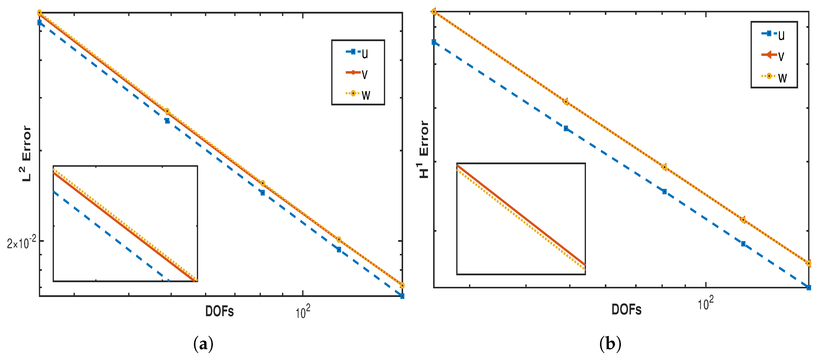
Figure 1a,b affirm the order convergence achieved in both norms
and
for variables
, and
w. The following
Table 1,
Table 2 and
Table 3 present the errors in both the norms and space convergence rate for all the variables.
Here, we numerically illustrate the attraction–repulsion chemotaxis dynamics of a cell population, providing visual insight into the behavior and interaction patterns governed by the system. These simulations serve to enhance our understanding of how the combined effects of chemoattractants and chemorepellents influence cell movement and aggregation.
For the purpose of demonstration, we selected specific model parameters that highlight key features of the system’s behavior. These parameters are assumed to reflect biologically relevant conditions and ensure numerical stability. The following values are used in our simulations:
with the initial conditions
in
. We choose time step
for the simulation.
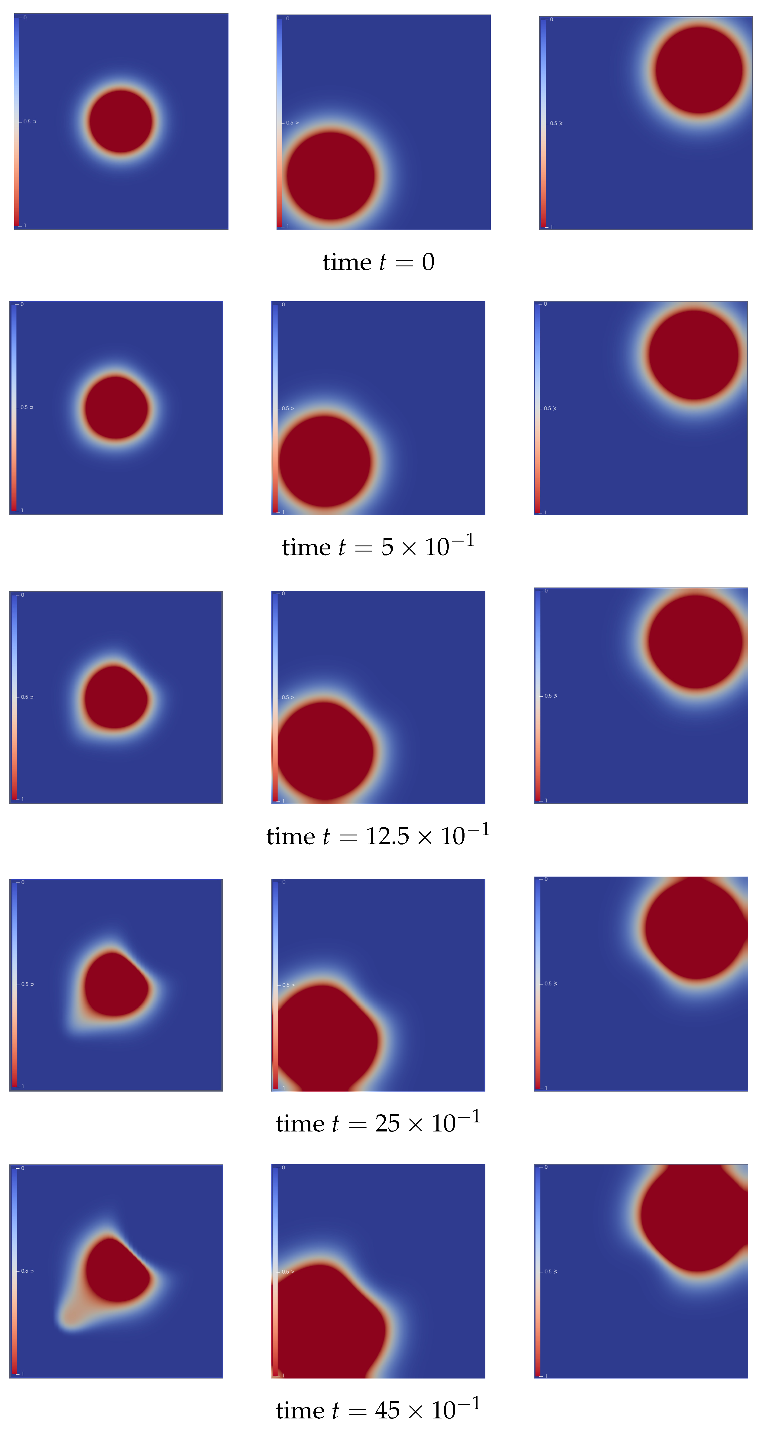
The following numerical illustration clearly demonstrates the movement of the cell population in our case bacteria population in response to nutrients and toxins. At the initial time
, we modeled our cell population
u as a circular cluster located at the center of the domain. The attractant signal (nutrient) is positioned at the bottom left corner, while the repellent (toxin) is placed at the top right corner of the domain; see the first row of
Figure 2. As time progresses, influenced by both the attraction and repulsion from these corner signals, the cells
u begin to diffuse away from the repellent
w and toward the attractant
v. The chemicals also start to diffuse across the domain after a certain period.
At time step
, the diffusion of the cell population is observed towards the bottom left corner of the domain, where the attractant chemical is becoming visible in the illustration. In contrast, the cell density at the top right corner appears to be lower than the initial data due to diffusion away from the toxin. The plots at this time step clearly show that cells are beginning to migrate away from the toxin and are diffusing towards the nutrient. Additionally, both chemicals have also started to diffuse in response to the cell movement; see the second and third rows of
Figure 2.
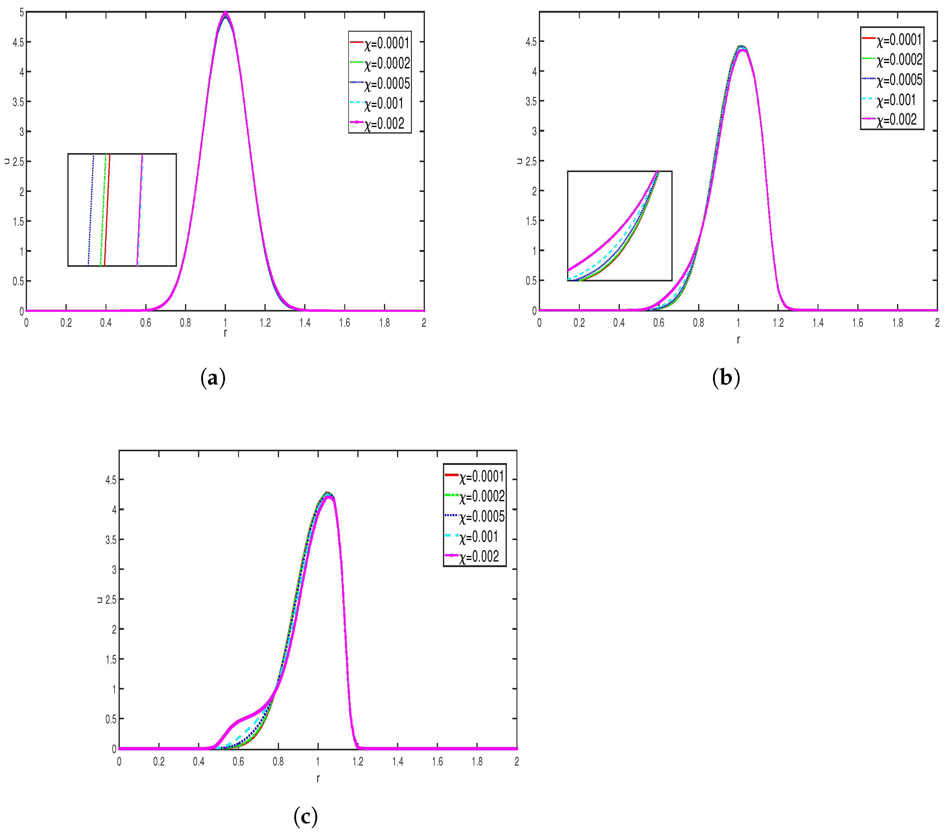
Figure 3 illustrates the evolution of cell density
u for different values of the chemical sensitivity coefficient
:
and
. This is presented for three different time steps. In this simulation, we considered other parameter values such as
for the various
values. From
Figure 3a, we can observe that, even across different time steps, all the curves reach their peak near
, although there are slight variations in shape. The zoomed-in images reveal a subtle shift in the curves as the value of
increases. From
Figure 3b,c it is evident that over time, while the peaks are consistently located in the same region, the shapes of the curves for different
values become more pronounced. As the attractant signal (nutrient) becomes dominant, the cells begin to aggregate or diffuse around the peak.
The above simulation represents the variation in the density of bacteria population for different values of the chemical sensitivity coefficient of toxins
,
with other parameters taken as
From the observations, we see that at the initial time, the curves reach their peak near
. The peak is slightly sharper in
Figure 4a compared to
Figure 4b. As time progresses, the coefficient of chemical sensitivity to the attractant remains constant, while repulsion becomes dominant, leading to deviations in the curves. An increase in repellent sensitivity forces the cells to disperse more, causing the peak of the curve to flatten in
Figure 4b compared to
Figure 4a. Overall, these images illustrate that as repellent sensitivity increases, the cells begin to diffuse away from areas of a high repellent concentration.
Effects of : The above simulation in
Figure 5 represents the variation in the diffusion of cell (bacteria) density with various values of diffusion coefficient, where other parameters are taken as
It is evident that around
there is a surge in the value of
u. We can see that in
Figure 5a, for a lower value of the diffusion coefficient, there is a higher concentrated accumulation near the center of the domain, which indicates that the diffusion is less, and as the value increases, the maximum value decreases and the curves become broader, indicating enhanced diffusion effects. Similar effects can be seen in
Figure 5b,c. As the time increases, for higher values of diffusion coefficients, the curves are seen to be broader and the maximum value is far less compared to the initial time, which indicates that the diffusion is more and dominates the chemotaxis.
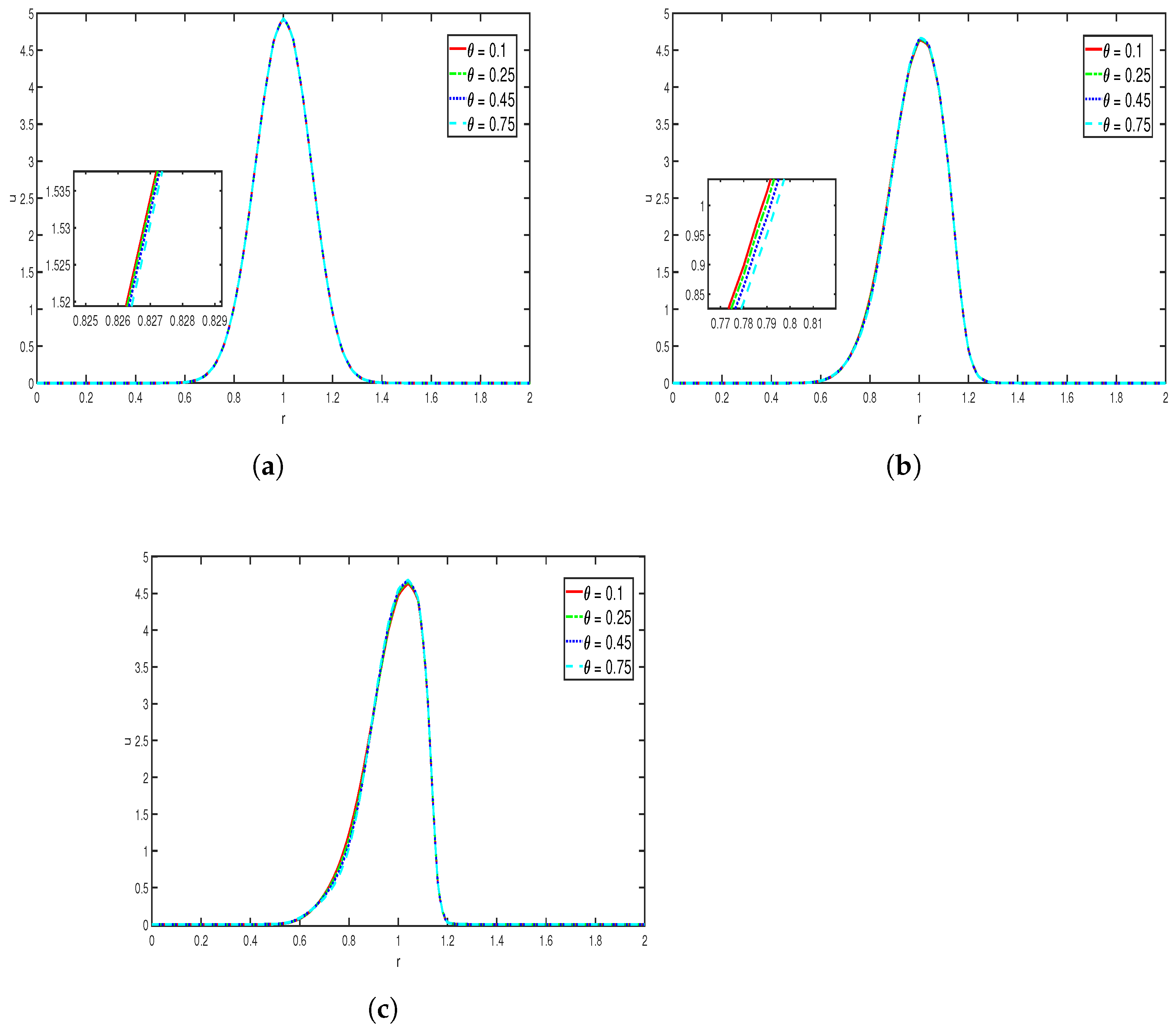
Effects of in cell density:
Figure 6 represents the timely variation in cell density
u for different values of the rate of consumption of nutrients—
—while other parameters are taken as follows:
The simulation results show the rate at which the nutrient is consumed by the bacteria (cell). Here,
has an effect on the bacteria (cell) aggregation. We can observe that as
and time increase, there is a subtle but noticeable shift in the position of the maximum value and amplitude of the cell density. In
Figure 6a,b the shift is not seen prominently, but in
Figure 6c, it is more visible. This suggests that as the consumption of nutrient increases, the cell aggregation becomes more focused. Overall, the above simulation indicates that even a small change in the chemical consumption rate can influence the diffusion and aggregation of cells.
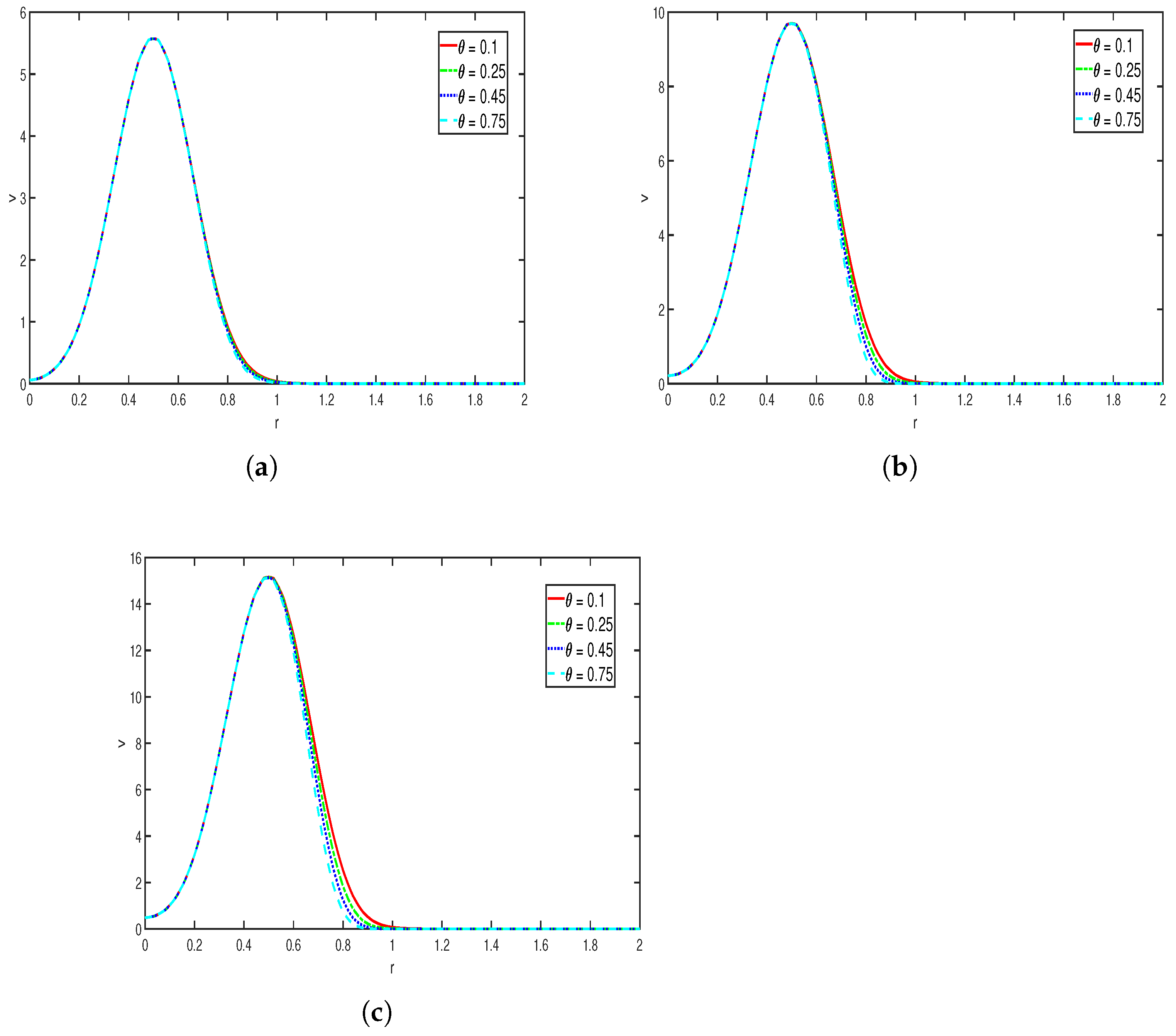
Effects of in concentration:
Figure 7 represents the variation in the nutrient concentration at 3 distinct time instances, where the values of other parameters are taken as
The parameter
represents the rate at which the nutrient is consumed by the bacteria (cells). As the value of
increases, the concentration of the nutrient decreases rapidly, leading to a more sharper decay in the chemical profile. The effect is visible in the plots. In
Figure 7a–c, for different values of
, the position at which the maximum is attained is seen to be relatively fixed; only the maximum value changes over time, which suggests that the primary effects of consumption are mainly on the rate of the depletion of nutrient rather than the location at which it is concentrated. Overall, the simulation shows that as the rate of consumption of nutrient increases, the nutrient concentration decays rapidly, resulting in narrower and steeper nutrient profiles, which show the sensitivity of the chemical signal towards the consumption rate.
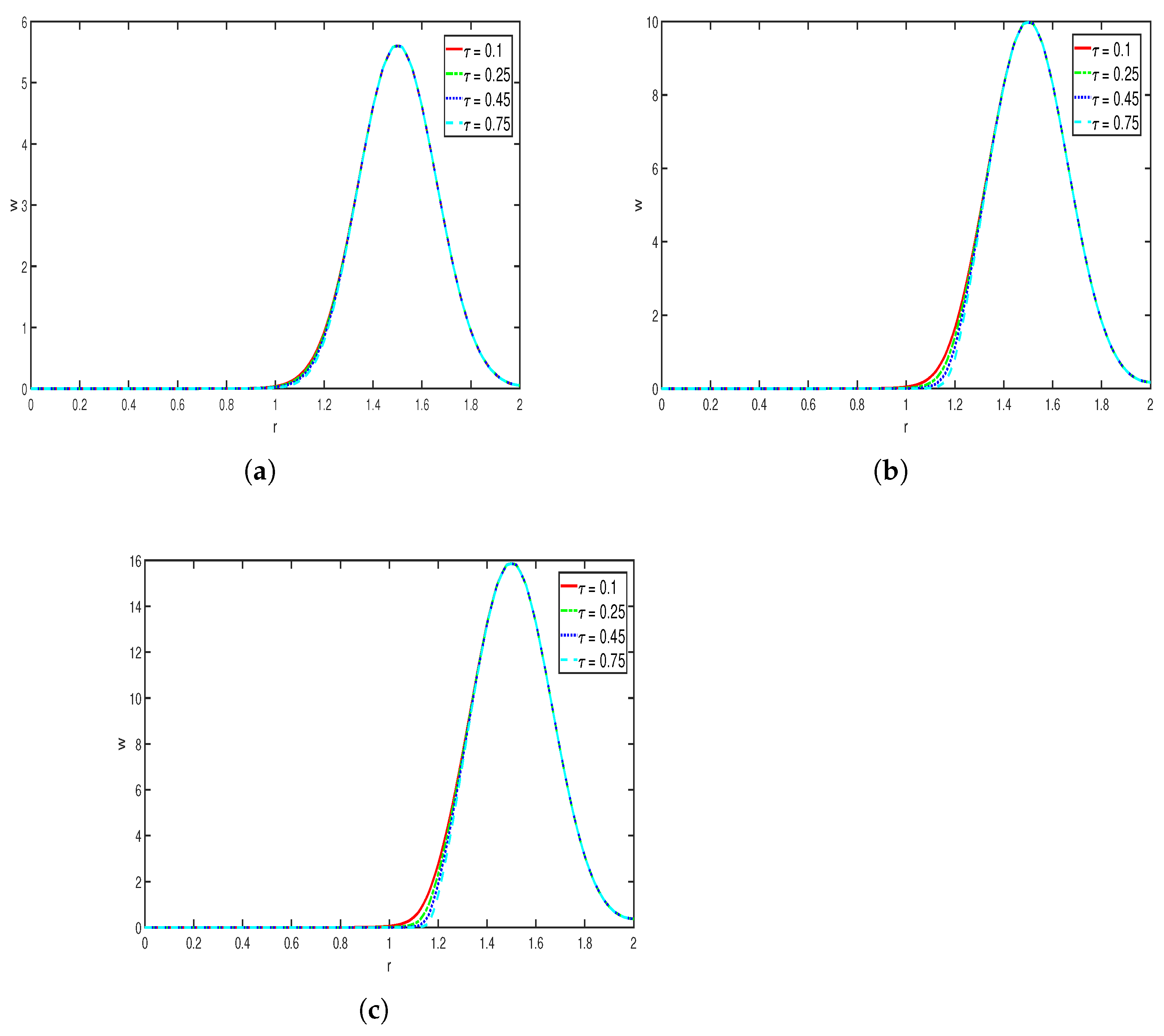
Effects of :
Figure 8 represents the evolution of toxin
w at different time steps, where the other parameters are taken as
As the consumption rate
of toxin increases, the toxin concentration profile becomes steeper and sharper. Specifically, large values of
lead to a faster consumption of the repellent chemical concentration, so the effect that the toxin has on the cell (bacteria) density may also decrease. We can see from
Figure 8a–c that although the location at which the maximum value is attained remains relatively constant, as time progresses, the sharpness and the steepness of the curve increase, with higher values of
. Overall, in this simulation we observe that the concentration of toxin (repellent)
w is highly sensitive to the chemical consumption rate.


 ,
, 


