
A Heuristic Approach to Competitive Facility Location via Multi-View K-Means Clustering with Co-Regularization and Customer Behavior

Abstract
1. Introduction
- It captures richer customer and facility representations by jointly leveraging geographic and preference data.
- It reveals latent patterns that are not discernible within any single view—for example, clusters with distinct preference profiles despite spatial proximity.
- It enforces alignment between views through co-regularization, thereby yielding clusters that are meaningful across multiple data dimensions.
- It provides robustness against noise or missing values in individual views by using complementary information from others.
- It supports decision interpretability by producing clusters grounded in both geographic and behavioral factors.
2. Related Work
3. Problem Statement and Mathematical Model
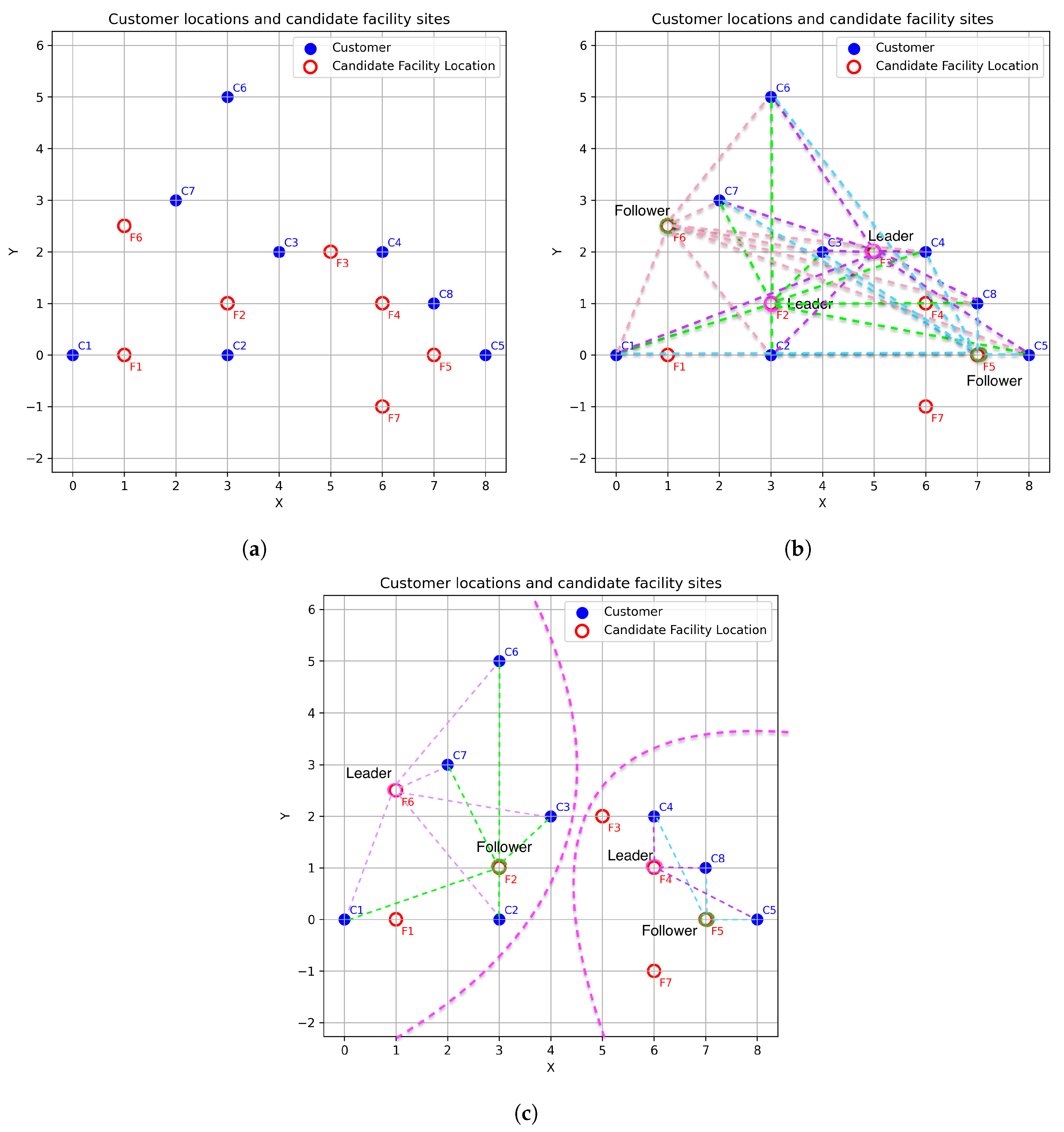
3.1. Motivating Example
3.2. Proposed Bilevel Optimization Model with Preference-Aware Attraction
3.3. Linear Reformulation of the Follower Problem
3.4. Theoretical Equivalence of the Reformulated Model
- Step 1: Recovering the structure of the nonlinear objective from MILP constraints.
- Step 2: Establishing optimality via contradiction.
3.5. Numerical Illustration of Preference Similarity
4. Algorithmic Framework
4.1. Multi-View K-Means Clustering with Co-Regularization
| Algorithm 1: Generalized multi-view K-means clustering with co-regularization |
Input: : V views of the data, each ; K: Number of clusters; : Co-regularization penalty for each view v; max_iter: Maximum number of iterations; Output: Final unified cluster assignments and centroids for each view v.  |
| Algorithm 2: Generalized optimization assignment with minimum facility constraint |
Input : Final cluster labels from Algorithm 1; Dataset D with facility and customer data; View matrices ; Optimization model ; Required minimum number of facilities per cluster m. Output: For each cluster k, the optimal facility locations assigned to the leader and follower, denoted as and , respectively. 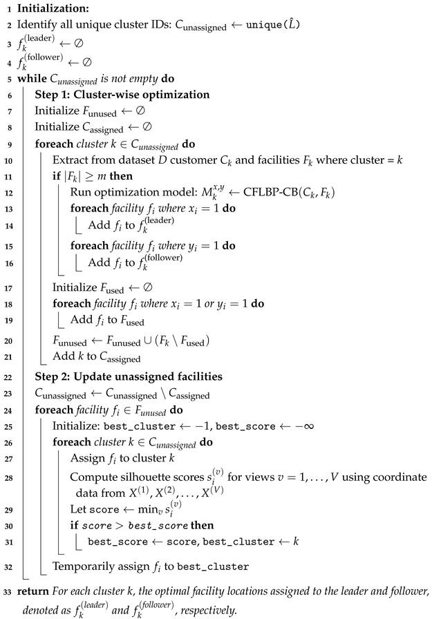 |
- is the average distance from point i to all other points in the same cluster;
- is the average distance from point i to all points in the nearest neighboring cluster.
- Step 1: Initialization
- Step 2: Iterative clustering process
- Step 2.1: Assignment step
- Step 2.2: Centroid update step
- Step 3: Post-processing (majority voting and silhouette tie-breaking)
4.2. Optimization Assignment
5. Case Study
5.1. Franchise Expansion into New Territories
5.2. Results
5.2.1. Clustering Results
5.2.2. Bilevel Optimization Results
5.2.3. Sensitivity of Multi-View K-Means Clustering to Co-Regularization Parameters
5.2.4. Parameter Tuning
5.2.5. Results from Single-View Clustering
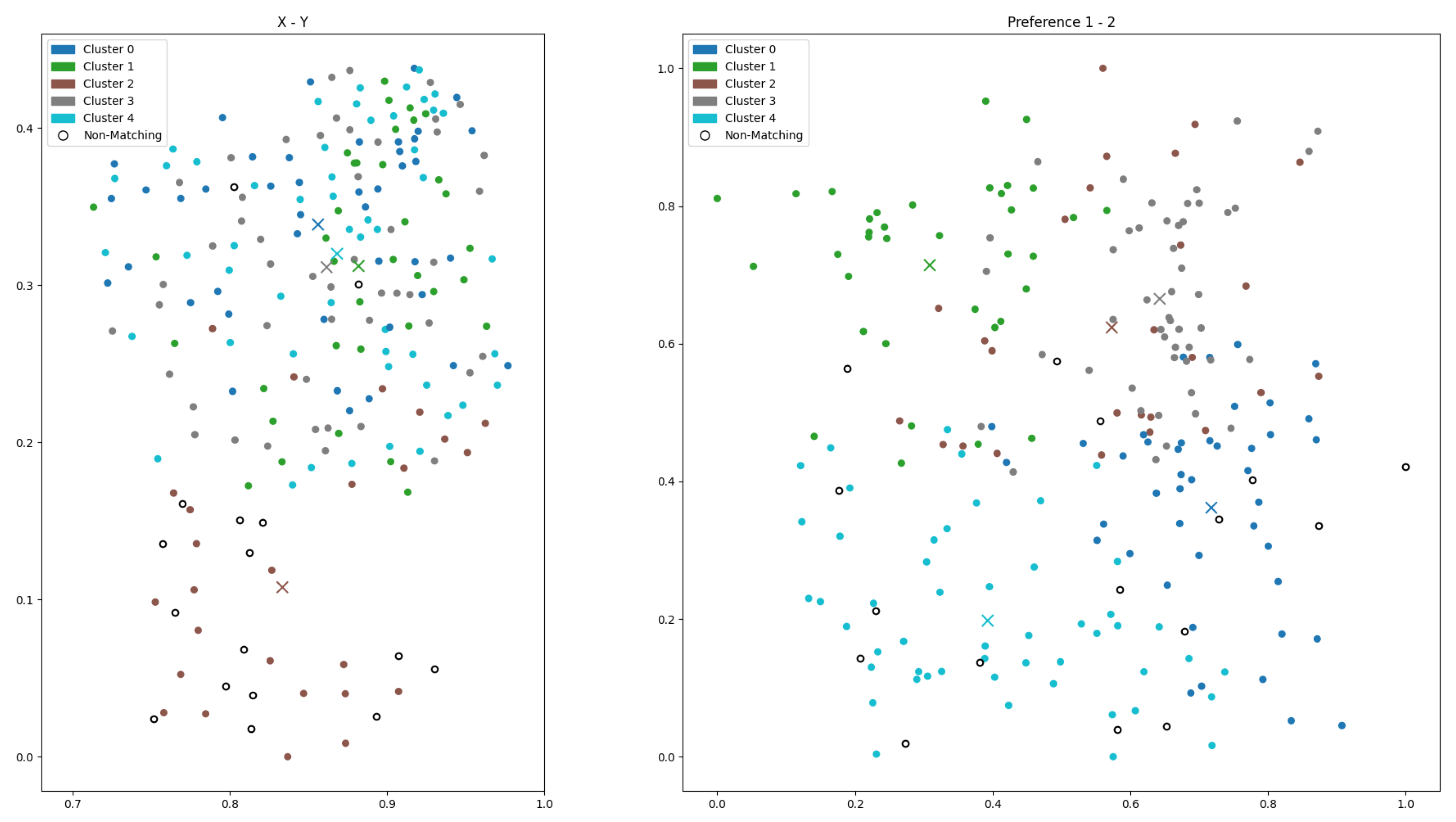
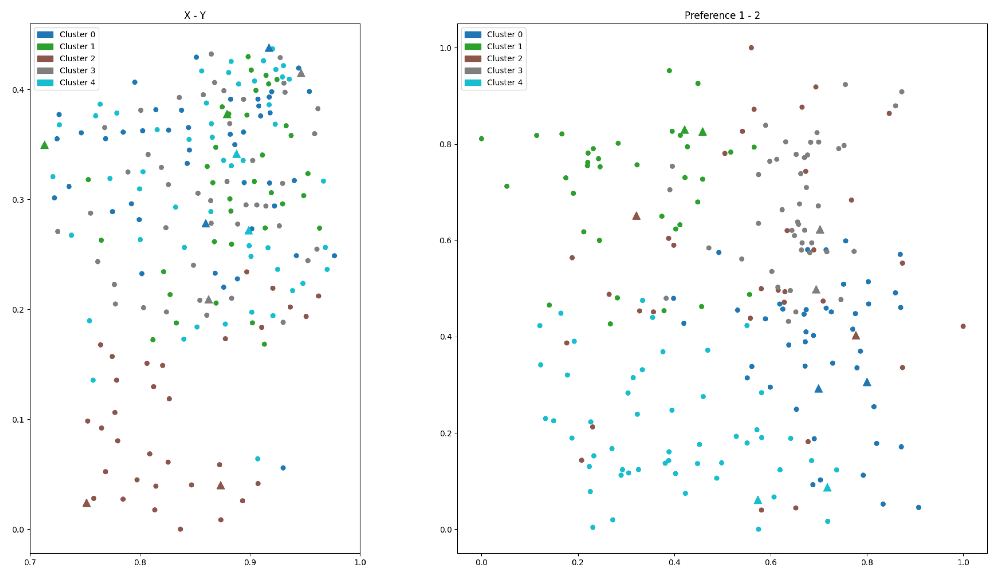
- Subplot (a): Geographic features (2D). Clustering based on geographic attributes yields compact and well-separated spatial clusters. Facility placements (triangles) are centrally located within their respective clusters, supporting strong geographic accessibility. However, the corresponding preference view exhibits substantial overlap among clusters, indicating poor alignment with customer preferences.
- Subplot (b): Preference features (2D).Clustering in the preference domain produces distinct and well-separated clusters, with facility locations closely aligned with preference centers. Nevertheless, the geographic projection reveals spatial dispersion and overlap, which may hinder efficient service delivery and cost-effective deployment.
- Subplot (c): Combined geographic and preference features (4D). The integration of both feature types leads to incoherent clustering in the spatial view, with facilities misaligned and positioned far from cluster centers. While the preference view maintains some alignment, overall cluster quality deteriorates.
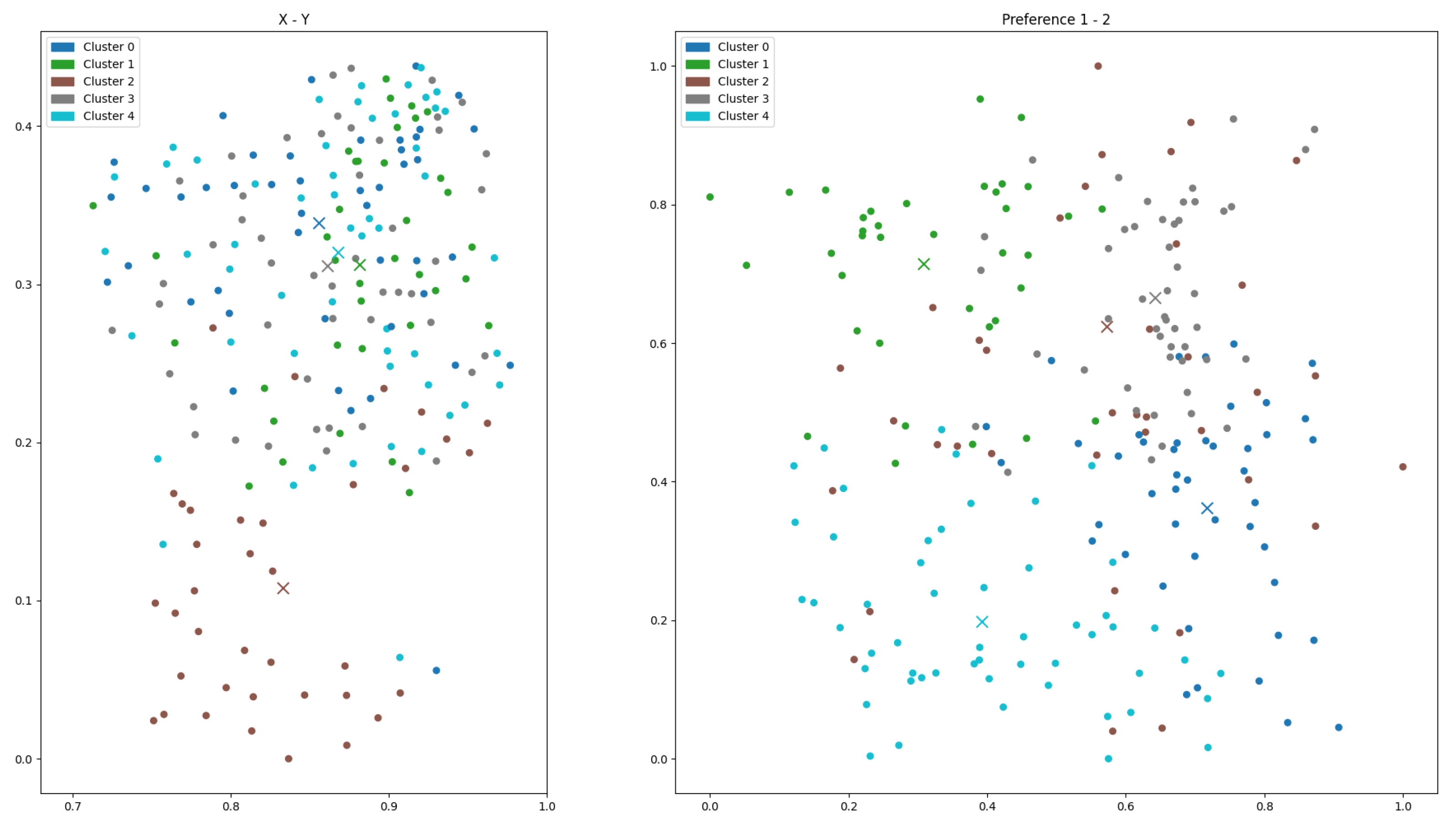
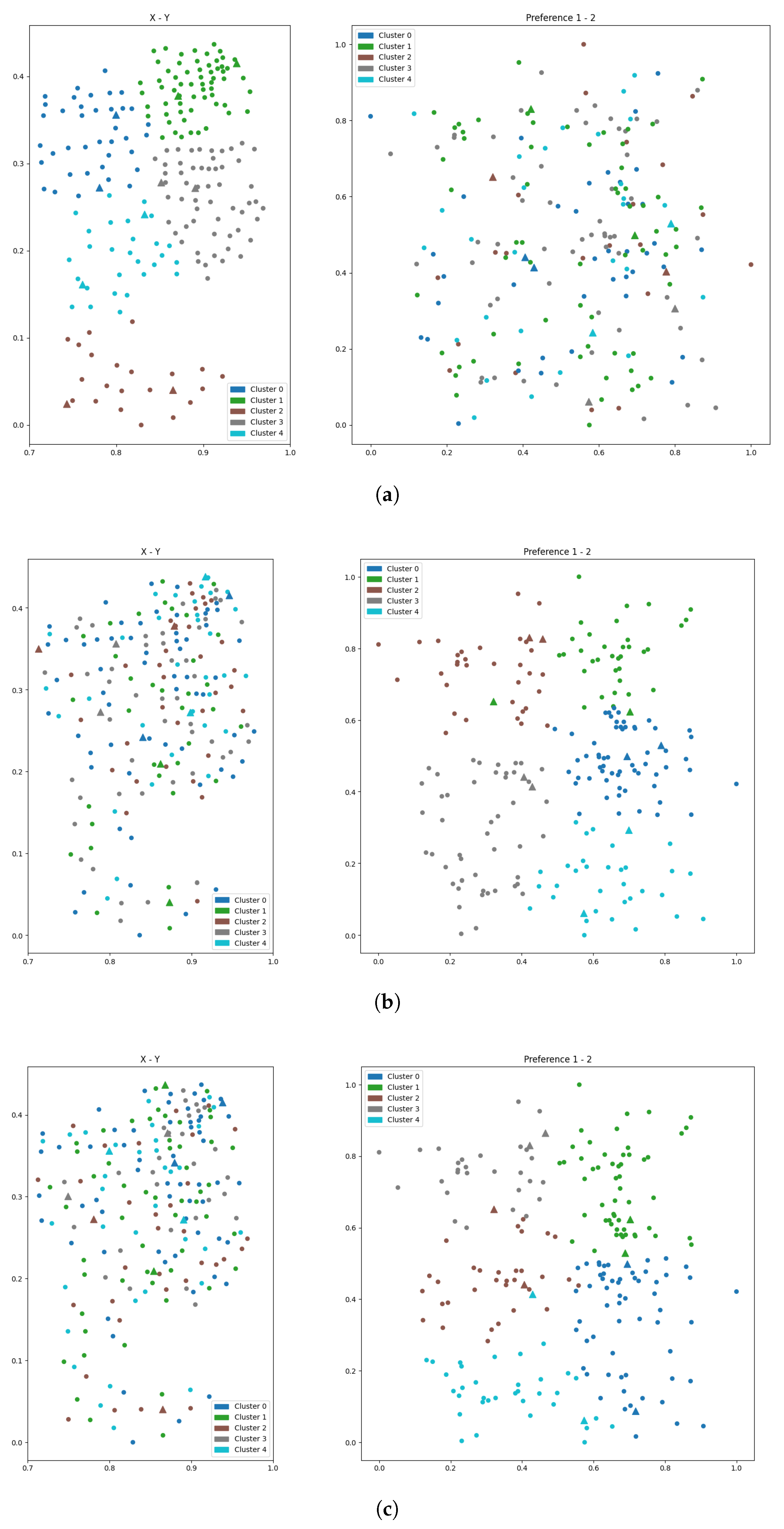
- Subplot (a): Geographic features (2D). Clustering based on geographic attributes results in well-separated spatial clusters, with facilities (triangles) embedded within each group, supporting accessibility. However, the corresponding preference view reveals significant cluster mixing, indicating poor alignment with customer behavioral attributes.
- Subplot (b): Preference features (2D). Clustering in the preference domain produces clearly defined clusters and well-aligned facilities, demonstrating effective segmentation. Yet the spatial projection shows considerable dispersion and overlap, reducing efficiency in physical service delivery.
- Subplot (c): Combined geographic and preference features (4D).The combined feature input yields scattered and incoherent clusters in both spatial and preference views, with facilities often located far from cluster centers, suggesting poor integration of the two feature spaces.
- Subplot (a): Geographic features (2D).The clustering results exhibit compact and spatially coherent groups. Facilities (triangles) are centrally located within clusters, enhancing spatial accessibility. However, in the corresponding preference space, clusters display substantial overlap, reflecting poor alignment with customer preferences.
- Subplot (b): Preference features (2D). The preference view reveals reasonably well-separated clusters, and most facility placements align with the cluster centers. An exception is Cluster 4, where the facility is not centrally located, indicating inconsistency. Meanwhile, the spatial view shows scattered and overlapping clusters, undermining geographic efficiency.
- Subplot (c): Combined geographic and preference features (4D). Clusters appear poorly defined in both spatial and preference views. Facility placements are inconsistently positioned and often located far from the respective cluster centers, reducing both behavioral targeting and spatial coverage.
5.2.6. Results from Multi-View K-Means Clustering
5.2.7. Comparison Between Single-View and Multi-View K-Means Clustering Results
- Multi-view clustering effectively integrates complementary spatial and behavioral patterns, yielding better facility–customer groupings for optimization.
- Co-regularization provides a tunable mechanism to balance intra-view fidelity and inter-view consistency, improving clustering quality and optimization outcomes.
- Despite slightly increased clustering overhead, the total computation time is reduced due to more efficient optimization on coherent clusters.
6. Discussion
6.1. Effectiveness of Multi-View Clustering
6.2. Insights from Co-Regularization Sensitivity
6.3. Comparison of Computational Efficiency with Bilevel Optimization
6.4. Evaluating Clustering-Induced Profit Bias
6.5. Comparative Metaheuristic: Genetic Algorithm
6.6. Comparative Evaluation of Optimization Methods
6.7. Implications for Competitive Facility Planning
6.8. Limitations and Future Work
7. Conclusions and Future Work
Author Contributions
Funding
Institutional Review Board Statement
Informed Consent Statement
Data Availability Statement
Acknowledgments
Conflicts of Interest
Notation and Definition
| I | Set of potential facility locations, indexed by . |
| J | Set of customers, indexed by . |
| p | Number of facilities to be opened by the leader. |
| r | Number of facilities to be opened by the follower. |
| Demand of customer j, representing the maximum potential turnover that can be captured by a serving facility. | |
| Distance between facility location i and customer j. | |
| Preference similarity ratio between facility i and customer j. | |
| Attraction coefficient combining spatial proximity (via inverse distance) and | |
| behavioral similarity (via ), defined as . | |
| A small positive constant used to avoid division by zero. | |
| Binary variable equal to 1 if the leader opens a facility at location i; | |
| 0 otherwise. | |
| Binary variable equal to 1 if the follower opens a facility at location i; | |
| 0 otherwise. |
References
- Drezner, T. A Review of Competitive Facility Location in the Plane. Logist. Res. 2014, 7, 114. [Google Scholar] [CrossRef]
- Eiselt, H.A.; Marianov, V.; Drezner, T. Competitive Location Models. In Location Science; Laporte, G., Nickel, S., Saldanha da Gama, F., Eds.; Springer International Publishing: Cham, Switzerland, 2020; pp. 391–429. [Google Scholar]
- ReVelle, C.; Eiselt, H.; Daskin, M. A Bibliography for Some Fundamental Problem Categories in Discrete Location Science. Eur. J. Oper. Res. 2008, 184, 817–848. [Google Scholar] [CrossRef]
- Fernández, P.; Pelegrín, B.; Lančinskas, A.; Žilinskas, J. New Heuristic Algorithms for Discrete Competitive Location Problems with Binary and Partially Binary Customer Behavior. Comput. Oper. Res. 2017, 79, 12–18. [Google Scholar] [CrossRef]
- Grohmann, S.; Urošević, D.; Carrizosa, E.; Mladenović, N. Solving Multifacility Huff Location Models on Networks Using Metaheuristic and Exact Approaches. Comput. Oper. Res. 2017, 78, 537–546. [Google Scholar] [CrossRef]
- Fernández, J.; Boglárka, G.; Redondo, J.L.; Ortigosa, P.M. The Probabilistic Customer’s Choice Rule with a Threshold Attraction Value: Effect on the Location of Competitive Facilities in the Plane. Comput. Oper. Res. 2019, 101, 234–249. [Google Scholar] [CrossRef]
- Serra, D.; Eiselt, H.A.; Laporte, G.; ReVelle, C.S. Market Capture Models under Various Customer-Choice Rules. Environ. Plan. B Plan. Des. 1999, 26, 741–750. [Google Scholar] [CrossRef]
- Drezner, T.; Drezner, Z. Finding the Optimal Solution to the Huff-Based Competitive Location Model. Comput. Manag. Sci. 2004, 1, 193–208. [Google Scholar] [CrossRef]
- Fernández, P.; Pelegrín, B.; Lančinskas, A.; Žilinskas, J. Exact and Heuristic Solutions of a Discrete Competitive Location Model with Pareto-Huff Customer Choice Rule. J. Comput. Appl. Math. 2021, 385, 113200. [Google Scholar] [CrossRef]
- Campos, C.M.; Santos-Peñate, D.R.; Moreno, J.A. An Exact Procedure and LP Formulations for the Leader–Follower Location Problem. TOP 2010, 18, 97–121. [Google Scholar] [CrossRef]
- Pelegrín, B.; Fernández, P.; García, M.D. On Tie Breaking in Competitive Location under Binary Customer Behavior. Omega 2015, 52, 156–167. [Google Scholar] [CrossRef]
- Plastria, F. Static Competitive Facility Location: An Overview of Optimisation Approaches. Eur. J. Oper. Res. 2001, 129, 461–470. [Google Scholar] [CrossRef]
- Plastria, F.; Vanhaverbeke, L. Discrete Models for Competitive Location with Foresight. Comput. Oper. Res. 2008, 35, 683–700. [Google Scholar] [CrossRef]
- Farahani, R.Z.; Abedian, M.; Sharahi, S. Competitive Facility Location. In Facility Location: Concepts, Models, Algorithms and Case Studies; Farahani, R.Z., Hekmatfar, M., Eds.; Springer: Berlin, Germany, 2009; pp. 347–372. [Google Scholar]
- Shan, W.; Yan, Q.; Chen, C.; Zhang, M.; Yao, B.; Fu, X. Optimization of Competitive Facility Location for Chain Stores. Ann. Oper. Res. 2019, 273, 187–205. [Google Scholar] [CrossRef]
- Zhou, L.; Du, G.; Lü, K.; Wang, L.; Du, J. A Survey and an Empirical Evaluation of Multi-View Clustering Approaches. ACM Comput. Surv. 2024, 56, 187. [Google Scholar] [CrossRef]
- Yang, Y. Protecting Attributes and Contents in Online Social Networks. Ph.D. Thesis, University of Kansas, Lawrence, KS, USA, 2014. [Google Scholar]
- Ye, F.; Chen, Z.; Qian, H.; Li, R.; Chen, C.; Zheng, Z. New Approaches in Multi-View Clustering. In Recent Applications in Data Clustering; IntechOpen: London, UK, 2018. [Google Scholar] [CrossRef]
- Hotelling, H. Stability in Competition. Econ. J. 1929, 39, 41–57. [Google Scholar] [CrossRef]
- Von Stackelberg, H. Marktform und Gleichgewicht; Springer: Berlin, Germany, 1934. [Google Scholar]
- Drezner, Z.; Eiselt, H.A. Competitive Location Models: A Review. Eur. J. Oper. Res. 2024, 316, 5–18. [Google Scholar] [CrossRef]
- Biesinger, B.; Hu, B.; Raidl, G. Models and Algorithms for Competitive Facility Location Problems with Different Customer Behavior. Ann. Math. Artif. Intell. 2016, 76, 93–119. [Google Scholar] [CrossRef]
- Casas-Ramírez, M.-S.; Camacho-Vallejo, J.-F. Solving the p-Median Bilevel Problem with Order through a Hybrid Heuristic. Appl. Soft Comput. 2017, 60, 73–86. [Google Scholar] [CrossRef]
- Kochetov, Y.; Kochetova, N.; Plyasunov, A. A Matheuristic for the Leader–Follower Facility Location and Design Problem. In Proceedings of the 10th Metaheuristics International Conference (MIC 2013), Singapore, 4–8 August 2013; Lau, H., Van Hentenryck, P., Raidl, G., Eds.; Citeseer: Princeton, NJ, USA, 2013; Volume 32, pp. 32/1–32/3. [Google Scholar]
- Rahmani, A.; Hosseini, M. A Competitive Stochastic Bi-Level Inventory Location Problem. Int. J. Manag. Sci. Eng. Manag. 2021, 16, 209–220. [Google Scholar] [CrossRef]
- Beresnev, V.L.; Melnikov, A.A. Computation of an Upper Bound in the Two-Stage Bilevel Competitive Location Model. J. Appl. Ind. Math. 2022, 16, 377–386. [Google Scholar] [CrossRef]
- Latifi, S.E.; Tavakkoli-Moghaddam, R.; Fazeli, E.; Arefkhani, H. Competitive Facility Location Problem with Foresight Considering Discrete-Nature Attractiveness for Facilities: Model and Solution. Comput. Oper. Res. 2022, 146, 105900. [Google Scholar] [CrossRef]
- Yu, W. Robust Competitive Facility Location Model with Uncertain Demand Types. PLoS ONE 2022, 17, e0273123. [Google Scholar] [CrossRef]
- Parvasi, S.P.; Taleizadeh, A.A.; Cárdenas-Barrón, L.E. Retail Price Competition of Domestic and International Companies: A Bi-Level Game Theoretical Optimization Approach. RAIRO-Oper. Res. 2023, 57, 291–323. [Google Scholar] [CrossRef]
- Zhou, Y.; Kou, Y.; Zhou, M. Bilevel Memetic Search Approach to the Soft-Clustered Vehicle Routing Problem. Transp. Sci. 2023, 57, 701–716. [Google Scholar] [CrossRef]
- Calvete, H.I.; Galé, C.; Iranzo, J.A.; Hernández, A. A Bilevel Approach to the Facility Location Problem with Customer Preferences under a Mill Pricing Policy. Mathematics 2024, 12, 3459. [Google Scholar] [CrossRef]
- Lin, Y.H.; Tian, Q.; Yu, Y. Bilevel Competitive Facility Location and Design under a Nested Logit Model. Comput. Oper. Res. 2024, 183, 107146. [Google Scholar]
- Legault, R.; Frejinger, E. A Model-Free Approach for Solving Choice-Based Competitive Facility Location Problems Using Simulation and Submodularity. INFORMS J. Comput. 2025, 37, 603–622. [Google Scholar] [CrossRef]
- Suárez-Vega, R.; Santos-Peñate, D.; García, D.P. Competitive Multifacility Location on Networks: The (r|Xp)-Medianoid Problem. J. Reg. Sci. 2004, 44, 569–588. [Google Scholar] [CrossRef]
- Kumar, A.; Rai, P.; Daumé, H. Co-Regularized Multi-View Spectral Clustering. Adv. Neural Inf. Process. Syst. 2011, 24, 1413–1421. [Google Scholar]
- Rousseeuw, P.J. Silhouettes: A Graphical Aid to the Interpretation and Validation of Cluster Analysis. J. Comput. Appl. Math. 1987, 20, 53–65. [Google Scholar] [CrossRef]


| Study | Objective Function | Solution Method | Application Domain |
|---|---|---|---|
| Drezner (2014) [1] | Maximize market share with location and quality differentiation | Bilevel model with best-response dynamics | Retail competition with quality-sensitive customers |
| Biesinger et al. (2017) [22] | Maximize market share with different types of customer behavior rules | MILP | Retail competition |
| Casas-Ramírez et al. (2017) [23] | Minimize the total cost between facility and customer | Reformulation of bilevel optimization to single-level optimization and heuristics | Retail competition, service networks |
| Kochetov et al. (2018) [24] | Maximize market share under proportional customer behavior | Bilevel MINLP, heuristics | Service networks |
| Rahmani et al. (2021) [25] | Maximize expected profit under demand uncertainty and competition | Branch-and-cut algorithm | Inventory and distribution systems |
| Beresnev et al. (2022) [26] | Maximize leader’s profit in a two-stage bilevel model | MILP reformulation to compute upper bound | Competitive retail location |
| Latifi et al. (2022) [27] | Maximize follower’s market share with discrete facility attractiveness and foresight | Bilevel integer programming with exact algorithm and dominance rules | Competitive retail location planning |
| Yu et al. (2022) [28] | Maximize leader’s market share under demand uncertainty | Two-stage robust optimization | Retail facility planning |
| Parvasi et al. (2023) [29] | Maximize domestic firm’s profit via price-setting competition | Bilevel game-theoretic optimization | International retail price competition |
| Zhou et al. (2023) [30] | Minimize total routing cost under soft customer clustering | Bilevel memetic algorithm with savings heuristic and local search | Logistics and vehicle routing |
| Calvete et al. (2024) [31] | Maximize net profit and total customer preference | Multi-objective optimization | Supply chain planning |
| Lin et al. (2024) [32] | Maximize own revenue considering nested customer preferences | Bilevel optimization, nested logit model | Retail stores, parcel lockers, park-and-ride stations |
| Legault et al. (2025) [33] | Maximize expected market share under random utility-based customer choice | Submodular optimization, simulation-based reformulation | Retail location with choice uncertainty |
| Demand | Supply | |||
|---|---|---|---|---|
| ID | Product Category 1 | Product Category 2 | Product Category 1 | Product Category 2 |
| () | () | () | () | |
| Customer 1 | 1.0 | 1.0 | — | — |
| Customer 2 | 0.8 | 0.9 | — | — |
| Customer 3 | 1.0 | 0.7 | — | — |
| Customer 4 | 0.9 | 0.9 | — | — |
| Facility 1 | — | — | 0.9 | 0.7 |
| Facility 2 | — | — | 0.8 | 0.9 |
| Facility 3 | — | — | 1.0 | 1.0 |
| Facility∖Customer | Customer 1 | Customer 2 | Customer 3 | Customer 4 |
|---|---|---|---|---|
| Facility 1 | 0.6300 | 0.7778 | 0.9000 | 0.7778 |
| Facility 2 | 0.7200 | 1.0000 | 0.8000 | 0.8889 |
| Facility 3 | 1.0000 | 1.0000 | 1.0000 | 1.0000 |
| Candidate Location | Latitude | Longitude |
|---|---|---|
| Location 1 | 37.7724 | –122.5100 |
| Location 2 | 37.7538 | –122.4889 |
| ⋮ | ⋮ | ⋮ |
| Location 16 | 37.7971 | –122.3989 |
| Customer ID | Latitude | Longitude | Population |
|---|---|---|---|
| 1 | 37.6508 | −122.4887 | 4135 |
| 2 | 37.6600 | −122.4835 | 4831 |
| ⋮ | ⋮ | ⋮ | ⋮ |
| 205 | 37.7823 | −122.4165 | 8188 |
| Cluster | Number of Customers | Number of Facilities |
|---|---|---|
| 0 | 43 | 2 |
| 1 | 35 | 2 |
| 2 | 32 | 5 |
| 3 | 44 | 5 |
| 4 | 51 | 2 |
| Clustering | Overall Profit | Leader Profit/Leader Market Share | Follower Profit | Follower Market Share |
|---|---|---|---|---|
| Equation (1) + Equation (10) | Equation (1) | Equation (10) | Equation (4) | |
| Cluster 0 | 3673.64 | 2394.47 | 1279.17 | 1905.52 |
| Cluster 1 | 3208.62 | 2421.07 | 787.55 | 1078.93 |
| Cluster 2 | 2152.80 | 1650.62 | 603.42 | 1650.62 |
| Cluster 3 | 3075.48 | 2430.24 | 645.24 | 1969.76 |
| Cluster 4 | 4307.10 | 2740.41 | 1566.69 | 2359.59 |
| Total profit | 16,417.64 | |||
| Time (s) | ||||
| Cluster | 0.1708 | |||
| Optimize | 2.9801 |
| Co-Regularization Parameters | Overall Profit | |
|---|---|---|
| 0.025 | 0 | 14,577.37 |
| 0.005 | 0.045 | 15,493.84 |
| 0.0025 | 0.105 | 15,279.92 |
| 0 | 0 | 15,812.44 |
| Clustering Feature View | Clustering Algorithm | Time (s) | Overall | Leader | Follower | |
|---|---|---|---|---|---|---|
| Cluster | Optimize | Profit | Profit | Profit | ||
| Geographic Only (2D) | K-means | |||||
| Cluster 0 | 2487.71 | 1646.93 | 840.78 | |||
| Cluster 1 | 4492.30 | 3514.33 | 977.96 | |||
| Cluster 2 | 1748.42 | 1109.41 | 639.01 | |||
| Cluster 3 | 4717.91 | 2945.07 | 1772.84 | |||
| Cluster 4 | 2116.53 | 1503.62 | 612.91 | |||
| Total profit | 0.0349 | 3.1019 | 15,562.87 | 10,719.37 | 4843.50 | |
| Preference Only (2D) | K-means | |||||
| Cluster 0 | 4115.54 | 3336.64 | 778.90 | |||
| Cluster 1 | 2587.65 | 2342.99 | 244.66 | |||
| Cluster 2 | 2695.60 | 2229.22 | 466.38 | |||
| Cluster 3 | 3894.70 | 2351.02 | 1543.69 | |||
| Cluster 4 | 2267.66 | 1607.27 | 660.39 | |||
| Total profit | 0.0604 | 4.6191 | 15,561.16 | 11,867.13 | 3694.03 | |
| Geographic + Preference (4D) | K-means | |||||
| Cluster 0 | 3706.87 | 3031.13 | 675.74 | |||
| Cluster 1 | 3746.44 | 2993.62 | 752.82 | |||
| Cluster 2 | 2554.85 | 1895.87 | 658.98 | |||
| Cluster 3 | 1944.56 | 1016.50 | 928.06 | |||
| Cluster 4 | 2452.30 | 1783.51 | 668.79 | |||
| Total profit | 0.0665 | 4.9162 | 14,405.02 | 10,720.63 | 3684.39 | |
| Geographic Only (2D) | Spectral | |||||
| Cluster 0 | 4418.97 | 3640.63 | 778.34 | |||
| Cluster 1 | 3622.13 | 2663.59 | 958.54 | |||
| Cluster 2 | 2617.91 | 1620.06 | 997.84 | |||
| Cluster 3 | 1988.18 | 1241.54 | 746.64 | |||
| Cluster 4 | 2348.86 | 1888.13 | 460.73 | |||
| Total profit | 0.0363 | 4.6648 | 14,996.05 | 11,053.95 | 3942.10 | |
| Preference Only (2D) | Spectral | |||||
| Cluster 0 | 5996.14 | 5313.10 | 683.04 | |||
| Cluster 1 | 2422.52 | 2061.96 | 360.57 | |||
| Cluster 2 | 2437.39 | 1972.63 | 464.76 | |||
| Cluster 3 | 2137.91 | 1384.10 | 753.81 | |||
| Cluster 4 | 2610.02 | 1707.89 | 902.14 | |||
| Total profit | 0.0330 | 6.3096 | 15,603.99 | 12,439.67 | 3164.32 | |
| Geographic + Preference (4D) | Spectral | |||||
| Cluster 0 | 2259.98 | 1645.98 | 614.00 | |||
| Cluster 1 | 2555.68 | 2189.37 | 366.32 | |||
| Cluster 2 | 4686.46 | 3531.55 | 1154.91 | |||
| Cluster 3 | 3180.11 | 1974.97 | 1205.14 | |||
| Cluster 4 | 2046.26 | 1486.62 | 559.64 | |||
| Total profit | 0.0330 | 6.3096 | 15,603.99 | 12,439.67 | 3164.32 | |
| Geographic Only (2D) | Hierarchical | |||||
| Cluster 0 | 4336.97 | 3398.04 | 938.92 | |||
| Cluster 1 | 3559.18 | 2648.60 | 910.57 | |||
| Cluster 2 | 2545.23 | 1745.23 | 800.00 | |||
| Cluster 3 | 1663.02 | 1055.61 | 607.41 | |||
| Cluster 4 | 3402.49 | 2345.99 | 1056.50 | |||
| Total profit | 0.0034 | 2.7864 | 15,292.71 | 10,979.30 | 4313.41 | |
| Preference Only (2D) | Hierarchical | |||||
| Cluster 0 | 3576.64 | 2175.02 | 1401.62 | |||
| Cluster 1 | 2784.32 | 1921.26 | 863.06 | |||
| Cluster 2 | 3359.66 | 2748.92 | 610.74 | |||
| Cluster 3 | 4460.88 | 3824.70 | 636.19 | |||
| Cluster 4 | 1311.06 | 1102.98 | 208.09 | |||
| Total profit | 0.0035 | 4.6121 | 15,376.47 | 11,534.48 | 3841.98 | |
| Geographic + Preference (4D) | Hierarchical | |||||
| Cluster 0 | 3789.64 | 2875.07 | 914.56 | |||
| Cluster 1 | 2553.21 | 1930.72 | 622.49 | |||
| Cluster 2 | 4141.97 | 2942.29 | 1199.68 | |||
| Cluster 3 | 2587.48 | 2101.52 | 485.96 | |||
| Cluster 4 | 1692.95 | 1267.86 | 425.09 | |||
| Total profit | 0.0035 | 4.5028 | 14,765.25 | 11,117.48 | 3647.77 | |
| Co-Regularization Parameters | Cluster | Leader Profit | Follower Profit | |
|---|---|---|---|---|
| 0.0225 | 0.075 | Cluster 0 | 2632.18 | 1389.18 |
| Cluster 1 | 2565.93 | 831.55 | ||
| Cluster 2 | 1557.11 | 600.06 | ||
| Cluster 3 | 1879.81 | 547.71 | ||
| Cluster 4 | 2740.41 | 1566.69 | ||
| Total profit | 16,310.62 | |||
| Time (s) | ||||
| Cluster | 0.1255 | |||
| Optimize | 3.0761 | |||
| 0.015 | 0.120 | Cluster 0 | 1993.43 | 1020.81 |
| Cluster 1 | 2899.40 | 873.65 | ||
| Cluster 2 | 2571.18 | 395.45 | ||
| Cluster 3 | 1776.11 | 700.12 | ||
| Cluster 4 | 2644.41 | 1444.39 | ||
| Total profit | 16,318.94 | |||
| Time (s) | ||||
| Cluster | 0.0915 | |||
| Optimize | 3.4215 | |||
| 0.025 | 0.015 | Cluster 0 | 2444.47 | 574.85 |
| Cluster 1 | 2037.71 | 1016.45 | ||
| Cluster 2 | 2725.75 | 1107.30 | ||
| Cluster 3 | 1318.40 | 726.50 | ||
| Cluster 4 | 2501.47 | 1338.96 | ||
| Total profit | 15,791.85 | |||
| Time (s) | ||||
| Cluster | 0.1001 | |||
| Optimize | 3.4982 | |||
| 0.000 | 0.000 | Cluster 0 | 2505.52 | 909.47 |
| Cluster 1 | 3522.01 | 1365.49 | ||
| Cluster 2 | 1711.16 | 869.78 | ||
| Cluster 3 | 2151.39 | 949.43 | ||
| Cluster 4 | 1192.56 | 635.64 | ||
| Total profit | 15,812.44 | |||
| Time (s) | ||||
| Cluster | 0.1750 | |||
| Optimize | 3.5193 | |||
| Clustering Feature View/ Co-Regularization Parameters | Clustering Algorithm | Time (s) | Overall | Leader | Follower | |
|---|---|---|---|---|---|---|
| Cluster | Optimize | Profit | Profit | Profit | ||
| Geographic Only (2D) | Single-view | 0.0349 | 3.1019 | 15,562.87 | 10,719.37 | 4843.50 |
| Preference Only (2D) | K-means clustering | 0.0604 | 4.6191 | 15,561.16 | 11,867.13 | 3694.03 |
| Geographic + Preference (4D) | 0.0665 | 4.9162 | 14,405.02 | 10,720.63 | 3684.39 | |
| Geographic Only (2D) | Single-view | 0.0363 | 4.6648 | 14,996.05 | 11,053.95 | 3942.10 |
| Preference Only (2D) | Spectral clustering | 0.0330 | 6.3096 | 15,603.99 | 12,439.67 | 3164.32 |
| Geographic + Preference (4D) | 0.0330 | 6.3096 | 15,603.99 | 12,439.67 | 3164.32 | |
| Geographic Only (2D) | Single-view | 0.0034 | 2.7864 | 15,292.71 | 10,979.30 | 4313.41 |
| Preference Only (2D) | Hierarchical clustering | 0.0035 | 4.6121 | 15,376.47 | 11,534.48 | 3841.98 |
| Geographic + Preference (4D) | 0.0035 | 4.5028 | 14,765.25 | 11,117.48 | 3647.77 | |
| Multi-view | 0.1708 | 2.9801 | 16,417.64 | 11,535.57 | 4882.07 | |
| K-means clustering | 0.1255 | 3.0761 | 16,310.62 | 11,375.44 | 4935.18 | |
| 0.0915 | 3.4215 | 16,318.94 | 11,884.53 | 4434.41 | ||
| 0.1001 | 3.4982 | 15,791.85 | 11,027.80 | 4764.05 | ||
| 0.1750 | 3.5193 | 15,812.44 | 11,082.64 | 4729.80 | ||
| Co-Regularization Parameters | Consistency | Silhouette | Cohesion | Profit | |||
|---|---|---|---|---|---|---|---|
| X–Y | Pref 1–2 | X–Y | Pref 1–2 | Framework | Full Model | ||
| 221 | 0.3505 | –0.0773 | 0.7393 | 1.5014 | 15,504.54 | 16,104.18 | |
| 165 | 0.0208 | 0.4059 | 0.6674 | 2.0014 | 14,969.93 | 16,071.82 | |
| 197 | 0.2074 | 0.0408 | 0.7008 | 1.6573 | 14,694.02 | 15,907.97 | |
| 120 | 0.3951 | 0.1509 | 0.7825 | 1.8579 | 15,638.27 | 15,882.79 | |
| 117 | 0.3374 | 0.1909 | 0.7744 | 1.8952 | 15,559.72 | 15,882.79 | |
| 126 | 0.1821 | 0.2854 | 0.7203 | 1.9347 | 15,742.97 | 15,835.59 | |
| 205 | 0.0073 | 0.1872 | 0.6565 | 1.8469 | 16,417.64 | 15,770.30 | |
| 103 | 0.1765 | 0.3914 | 0.715 | 1.997 | 15,548.17 | 15,758.24 | |
| 220 | 0.0274 | –0.0785 | 0.6563 | 1.5269 | 14,760.96 | 15,751.88 | |
| Evaluation Criteria | Correlation Coefficient |
|---|---|
| Overall objective | 0.2271 |
| Leader profit | 0.5868 |
| Follower profit | 0.2506 |
| Follower market share | 0.5868 |
| Generation | Evaluations | Average Overall Profit | Maximum Overall Profit | Time (Seconds) |
|---|---|---|---|---|
| 0 | 20 | 14,941.60 | 15,595.04 | 91.77 |
| 1 | 18 | 15,264.77 | 15,661.82 | 89.97 |
| 2 | 16 | 15,424.87 | 15,991.54 | 80.94 |
| 3 | 19 | 15,565.02 | 15,991.54 | 93.35 |
| 4 | 13 | 15,756.81 | 16,028.84 | 66.15 |
| 5 | 18 | 15,930.98 | 16,099.76 | 89.54 |
| 6 | 15 | 15,963.93 | 16,104.40 | 73.48 |
| 7 | 14 | 15,971.32 | 16,104.40 | 69.96 |
| 8 | 12 | 16,030.23 | 16,104.40 | 58.89 |
| 9 | 15 | 16,039.75 | 16,137.75 | 74.06 |
| Solution Framework | Co-Regularization | Time (s) | Overall | Leader | Follower | Follower | |
|---|---|---|---|---|---|---|---|
| Cluster | Optimize | Profit | Profit | Profit | Market Share | ||
| Multi-view framework | (0.0250, 0.0750) | 0.1708 | 2.9801 | 16,417.64 | 11,535.57 | 4882.07 | 8964.43 |
| Multi-view solution on full model | 15,770.30 | 11,390.20 | 4380.10 | 9109.80 | |||
| Multi-view framework | (0.0050, 0.1500) | 0.1042 | 3.8963 | 15,504.54 | 11,055.31 | 4449.22 | 9444.69 |
| Multi-view solution on full model | 16,104.17 | 11,798.48 | 4305.69 | 8701.51 | |||
| Direct CFLBP-CB | 608.5756 | 15,988.27 | 11,254.59 | 4733.68 | 9245.41 | ||
| GA | |||||||
| gen 6 | 585.2000 | 16,104.40 | 11,594.58 | 4509.82 | 8905.42 | ||
| gen 9 | 788.1100 | 16,137.75 | 11,872.01 | 4265.73 | 8627.98 | ||
Disclaimer/Publisher’s Note: The statements, opinions and data contained in all publications are solely those of the individual author(s) and contributor(s) and not of MDPI and/or the editor(s). MDPI and/or the editor(s) disclaim responsibility for any injury to people or property resulting from any ideas, methods, instructions or products referred to in the content. |
© 2025 by the authors. Licensee MDPI, Basel, Switzerland. This article is an open access article distributed under the terms and conditions of the Creative Commons Attribution (CC BY) license (https://creativecommons.org/licenses/by/4.0/).
Share and Cite
Phoka, T.; Poonprapan, P.; Boriwan, P. A Heuristic Approach to Competitive Facility Location via Multi-View K-Means Clustering with Co-Regularization and Customer Behavior. Mathematics 2025, 13, 2481. https://doi.org/10.3390/math13152481
Phoka T, Poonprapan P, Boriwan P. A Heuristic Approach to Competitive Facility Location via Multi-View K-Means Clustering with Co-Regularization and Customer Behavior. Mathematics. 2025; 13(15):2481. https://doi.org/10.3390/math13152481
Chicago/Turabian StylePhoka, Thanathorn, Praeploy Poonprapan, and Pornpimon Boriwan. 2025. "A Heuristic Approach to Competitive Facility Location via Multi-View K-Means Clustering with Co-Regularization and Customer Behavior" Mathematics 13, no. 15: 2481. https://doi.org/10.3390/math13152481
APA StylePhoka, T., Poonprapan, P., & Boriwan, P. (2025). A Heuristic Approach to Competitive Facility Location via Multi-View K-Means Clustering with Co-Regularization and Customer Behavior. Mathematics, 13(15), 2481. https://doi.org/10.3390/math13152481