One-Dimensional Shallow Water Equations Ill-Posedness

Abstract

In 2071, the Hydraulic community will commemorate the second centenary of the Baré de Saint-Venant equations, also known as the Shallow Water Equations (SWE). These equations are fundamental to the study of open-channel flow. As non-linear partial differential equations, their solutions were largely unattainable until the development of computers and numerical methods. Following 1960, various numerical schemes emerged, with Preissmann’s scheme becoming the most widely employed in many software applications. In the 1990s, some researchers identified a significant limitation in existing software and codes: the inability to simulate transcritical flow. At that time, Preissmann’s scheme was the dominant method employed in hydraulics tools, leading the research community to conclude that this scheme could not handle transcritical flow due to suspected instability. In response to this concern, several researchers suggested modifications to Preissmann’s scheme to enable the simulation of transcritical flow. This paper will demonstrate that these accusations against the Preissmann scheme are unfounded and that the proposed improvements are unnecessary. The observed instability is not due to the numerical method itself, but rather a mathematical instability inherent to the SWE, which can lead to ill-posed conditions if a specific derived condition is not met. In the context of a friction slope formula based on Manning or Chézy types, the condition for ill-posedness of the 1D shallow water equations simplifies to the Vedernikov number condition, which is necessary for roll waves to develop in uniform flow. This derived condition is also relevant for the formation of roll waves in unsteady flow when the 1D shallow water equations become ill-posed.

1. Introduction

In 2071, the Hydraulic community will mark the 200th anniversary of the one-dimensional Baré de Saint-Venant equations, also called the one-dimensional Shallow Water Equations (1D-SWE). These are non-linear hyperbolic PDEs. However, their mathematical properties have received limited research attention. Consequently, questions about the existence and uniqueness of solutions for full 1D-SWE remain largely unresolved. While many researchers have explored the 1D-SWE without considering the source term or only ignoring the friction source term (e.g., [1,2,3,4,5,6,7,8,9,10,11]), establishing well-posedness in these cases, no studies have focused specifically on the full 1D-SWE including the friction source term. Some argue that ignoring the complete source term is not critical, claiming that lower-order terms do not influence well-posedness. This study seeks to address this issue.

The development of computers and advances in numerical methods have made it more feasible to solve the 1D-SWE. Preissmann’s scheme [12], commonly used in various software and numerical tools for modeling unsteady flow (e.g., [13,14]), is effective but was suspected to have limitations. In the 1990s, some researchers (e.g., [15]) argued that this scheme is unsuitable for simulating transcritical flow in open channels, where both subcritical and supercritical flow regimes occur, leading to instability. Several alternative methods have been proposed to enhance stability [15,16,17,18]. For instance, ref. [17] notes the challenges: “The Preissmann box scheme is the standard numerical method employed by hydraulic engineers to model open channel flows or surcharged pipes; however, it fails for transcritical flows. Various alternatives exist, but we show how simple modifications to the difference scheme and solution method can enable its use for these flows.” Interestingly, before the first critique in [15], Samuels and Skeels in 1990 successfully used the Preissmann scheme to simulate transcritical flow at a Froude number below 1.5, concluding, “It is clear from these model results that supercritical flow was simulated without the numerical oscillations typically associated with transitions through the critical state” [19]. Unfortunately, this promising result was not further explored.

To tackle the difficulties of modeling transcritical flow, some researchers have adopted alternative numerical schemes, while others have adjusted the original equations. For example, Kutija and Newett [20] developed the NewC scheme and observed oscillations near a Froude number of 1.5 in large channels, signaling numerical instability. They addressed this by increasing numerical diffusion. AlQasimi and Mahdi [21] faced similar issues with their UMHYSER-1D software, which is based on the NewC scheme. Conversely, Yu et al. [22] introduced a “new reference slope form of the Saint-Venant equations” to maintain smooth slope source terms and reduce oscillations. They pointed out a key limitation: their study focused only on subcritical flow and noted that the SPRNT code, based on the Preissmann scheme, “is known to exhibit instabilities with transcritical flows. which can be mitigated using the ad hoc local partial inertia (LPI) scheme of Fread et al. (1996) [23]”. This LPI method alters the momentum equation of the 1D SWE by either decreasing or removing the convective term, resulting in a modified 1D SWE that is subcritical [23]. Although this method has been successfully used in various software (e.g., [24,25,26]), its mathematical soundness is questionable. The original 1D SWE are hyperbolic, but the modified version becomes parabolic, which leads to different domains of dependence and influence, thus diverging from the original problem. This approach is similar to regularization in ill-posed problems [27], but it fundamentally alters the problem’s nature, resulting in incorrect solutions.

This paper examines the fundamental question of the ill-posedness of the 1D SWE. In fact, when solving these non-linear PDEs, no one has verified their well-posedness; it has been assumed implicitly. The reason for this is that the 1D SWE are based on physical principles—namely, mass and momentum conservation—so they are presumed to be well-posed. However, this paper shows that the source term does affect the well-posedness of the 1D SWE. Furthermore, the conditions leading to the ill-posedness of the 1D SWE will be presented, along with the implications of this finding. The remainder of this paper is organized as follows: Section 2 introduces useful definitions and tools for the subsequent analysis. Section 3 describes the methodology used to determine the valid range of the Froude number for the 1D SWE. Section 4 presents the main results followed by discussion in Section 5, and conclusions in Section 6.

2. Mathematical Background

For completeness, this section summarizes the mathematical definitions and tools necessary for this paper. The differential problem, which is the 1D SWE supplemented with initial and/or boundary conditions, must be well-posed to allow for a solution.

2.1. Governing Equations

The 1D SWE, or Barré de St-Venant equations, expressed in terms of water depth and velocity (e.g., [28,29,30]), for river flows in prismatic channels, are:

$${\displaystyle \frac{𝜕h}{𝜕t}}+D{\displaystyle \frac{𝜕u}{𝜕x}}+u{\displaystyle \frac{𝜕h}{𝜕x}}=0$$

(1)

$${\displaystyle \frac{𝜕u}{𝜕t}}+u{\displaystyle \frac{𝜕u}{𝜕x}}+g{\displaystyle \frac{𝜕h}{𝜕x}}=g\left(S_0-S_f\right)$$

(2)

where u = flow velocity (m/s), h = water depth (m), D = A/T = hydraulic depth (m), A = wetted area (m²), T = top water surface width (m), g = gravity acceleration (m/s²), S₀ = bed slope (-), S_f = friction slope (-), t = time independent variable (s), and x = spatial independent variable (m).

These equations may incorporate extra terms and coefficients to account for wind stress, lateral flow, the nonuniformity of velocity distribution, and other factors [30]. In this paper, the fundamental form of the 1D SWE, Equations (1) and (2), is employed since the results are unaffected by additional modifications. The friction slope is expressed as [31]:

$$S_f=k u^r{R}^m$$

(3)

where $R$ = hydraulic radius (m), and k a coefficient. Manning equation corresponds to $k=n^2$, $r=2$, and $m=-4/3$, $n$ being the Manning coefficient, while $k=1/C^2$, $r=2$, and $m=-1$, with, $C$ being the Chézy coefficient, if Chézy equation is used.

In matrix form, Equations (1) and (2) take the form:

$${\displaystyle \frac{𝜕\mathit{U}}{𝜕t}}+\mathit{M}{\displaystyle \frac{𝜕\mathit{U}}{𝜕x}}=\mathit{S}$$

(4)

where

$$\mathit{U}=\left(\begin{array}{c}h\\ u\end{array}\right), \mathit{M}=\left(\begin{array}{cc}u& D\\ g& u\end{array}\right), \mathit{S}=\left(\begin{array}{c}0\\ g\left(S_0-S_f\right)\end{array}\right)$$

(5)

To be solved, Equation (4) requires initial conditions:

$$\mathit{U}\left(x,0\right)=\left(\begin{array}{c}v\left(x\right)\\ w\left(x\right)\end{array}\right)$$

(6)

Providing a purely Cauchy problem. If boundary conditions are included, it transforms into a mixed Cauchy problem. The characteristic form of the 1D SWE is given as (e.g., [30,32]):

$$\left\{\begin{array}{c}{\displaystyle \frac{𝜕(u+2\sqrt{gh})}{𝜕t}}+(u+\sqrt{gh}){\displaystyle \frac{𝜕(u+2\sqrt{gh})}{𝜕x}}=g\left(S_0-S_f\right)\\ {\displaystyle \frac{𝜕(u-2\sqrt{gh})}{𝜕t}}+(u-\sqrt{gh}){\displaystyle \frac{𝜕(u-2\sqrt{gh})}{𝜕x}}=g\left(S_0-S_f\right)\end{array}\right.$$

(7)

Or equivalently:

$$\left\{\begin{array}{c}{\displaystyle \frac{d\left(u+2\sqrt{gh}\right)}{dt}}=g\left(S_0-S_f\right) (a)\\ {\displaystyle \frac{dx}{dt}}=\left(u+\sqrt{gh}\right) (b)\end{array}\right.$$

(8)

And

$$\left\{\begin{array}{c}{\displaystyle \frac{d(u-2\sqrt{gh})}{dt}}=g\left(S_0-S_f\right) (a)\\ {\displaystyle \frac{dx}{dt}}=\left(u-\sqrt{gh}\right) (b)\end{array}\right.$$

(9)

Because the slopes of the characteristics, $\mathit{dx}/\mathit{dt}$ in Equations (8) and (9), are real and distinct, the 1D SWE are hyperbolic PDEs. If the source term is included, Riemann invariants do not exist. The slopes of the characteristic curves are unaffected by the source term itself. However, as shown by the compatibility relations, Equations (8) and (9), the source term influences the solution components u and h, which in turn modify the slopes of the characteristics. Therefore, the source term indirectly affects these slopes. In the linearized form of the equations, the characteristic slopes are constant and unaffected by the solution, although the source term still impacts the overall solution. The central question of this paper is: since the source term influences the solution, under what conditions do the 1D SWE become ill-posed?

2.2. Evolution of Internal Perturbations

The general form of a pure Cauchy problem for unsteady flow in a very long channel is described by the following equations:

$${\displaystyle \frac{𝜕\mathit{U}}{𝜕t}}+\mathit{M}{\displaystyle \frac{𝜕\mathit{U}}{𝜕x}}=\mathit{S}$$

(10)

$$\mathit{U}\left(x,0\right)=\left(\begin{array}{c}v\left(x\right)\\ w\left(x\right)\end{array}\right)$$

(11)

where

$$\mathit{U}=\left(\begin{array}{c}h\\ u\end{array}\right), \mathit{M}=\left(\begin{array}{cc}u& D\\ g& u\end{array}\right), \mathit{S}=\left(\begin{array}{c}0\\ g\left(S_0-S_f\right)\end{array}\right)$$

(12)

In the presence of perturbations of water depth and velocity, $h^{\prime }$ and $u^{\prime }$, the perturbed pure Cauchy problem is:

$${\displaystyle \frac{𝜕\tilde{\mathit{U}}}{𝜕t}}+\tilde{\mathit{M}}{\displaystyle \frac{𝜕\tilde{\mathit{U}}}{𝜕x}}=\tilde{\mathit{S}}$$

(13)

$$\tilde{\mathit{U}}\left(x,0\right)=\left(\begin{array}{c}v\left(x\right)+v^{\prime }\left(x\right)\\ w\left(x\right)+w^{\prime }\left(x\right)\end{array}\right)$$

(14)

where

$$\tilde{\mathit{U}}=\left(\begin{array}{c}\tilde{h}=h+h^{\prime }\\ \tilde{u}=u+u^{\prime }\end{array}\right)=\mathit{U}+{\mathit{U}}^{\prime }, \tilde{\mathit{M}}=\left(\begin{array}{cc}\tilde{u}=u+u^{\prime }& \tilde{D}=D+D^{\prime }\\ g& \tilde{u}=u+u^{\prime }\end{array}\right)=\mathit{M}+{\mathit{M}}^{\prime }, \tilde{\mathit{S}}=\left(\begin{array}{c}0\\ g\left(S_0-\widetilde{S_f}\right)\end{array}\right)$$

(15)

With:

$${\mathit{M}}^{\prime }=\left(\begin{array}{cc}{u}^{\prime }& D^{\prime }\\ 0& u^{\prime }\end{array}\right) \mathrm{and} {\mathit{U}}^{\prime }=\left(\begin{array}{c}{h}^{\prime }\\ u^{\prime }\end{array}\right)$$

(16)

As shown in Appendix A, the small perturbation field ${\mathit{U}}^{\prime }$ satisfies the following pure Cauchy problem:

$${\displaystyle \frac{𝜕{\mathit{U}}^{\prime }}{𝜕t}}+\mathit{M}{\displaystyle \frac{𝜕{\mathit{U}}^{\prime }}{𝜕x}}+\mathit{N}{\mathit{U}}^{\prime }=0$$

(17)

$${\mathit{U}}^{\prime }\left(x,0\right)=\left(\begin{array}{c}{v}^{\prime }\left(x\right)\\ w^{\prime }\left(x\right)\end{array}\right)$$

(18)

where

$${\mathit{U}}^{\prime }=\left(\begin{array}{c}{h}^{\prime }\\ u^{\prime }\end{array}\right), \mathit{M}=\left(\begin{array}{cc}u& D\\ g& u\end{array}\right), \mathit{N}=g\left(\begin{array}{cc}0& 0\\ {\displaystyle \frac{𝜕S_f}{𝜕h}}& {\displaystyle \frac{𝜕S_f}{𝜕u}}\end{array}\right)$$

(19)

The perturbation field satisfies a non-linear PDE, Equations (17) and (18). If this problem is ill-posed, then the perturbed one, Equations (13) and (14), will also be ill-posed since $\tilde{\mathit{U}}=\mathit{U}+{\mathit{U}}^{\prime }$, Equation (15).

2.3. Principle of Frozen Coefficients

The key question is whether small initial perturbations, as given by Equation (18), will grow over time. Mathematically, this can only be determined if the problem described by Equations (17) and (18) is linear. However, since the matrices $\mathit{M}$ and $\mathit{N}$ depend on the original water depth and velocity, which makes the problem non-linear, the “principle of frozen coefficients” ([33]; pp. 215–216) is used. This approach involves analyzing modified problems where the coefficients of the matrices are held constant at any chosen point,$(x_0,t_0)$, with water depth, hydraulic depth, and velocity designated as $h_0$, $D_0$ and $u_0$ respectively.

This principle involves deriving a series of linear problems from the original Equations (17) and (18) by fixing the coefficients of the matrices $\mathit{M}$ and $\mathit{N}$. These coefficients represent all possible solutions to the 1D SWE of the unperturbed flow, as described in Equations (10) and (11). The “principle of frozen coefficients” states that if the Cauchy problem is well-posed at all points $(x_0,t_0)$, then the original problem with variable coefficients should also be well-posed. Numerous researchers have examined the linearized 1D SWE using a uniform flow as the base state (e.g., [34,35,36]), indicating their conclusions are only valid near uniform flow conditions. For instance, Vedernikov’s well-known paper [34] states a condition for uniform flow stability. All researchers who investigated uniform flow stability using the 1D SWE concluded that the uniform flow is unstable, but no one mentioned the ill-posedness of the 1D SWE. In this work, applying the “principle of frozen coefficients” ensures that the results apply to any point in the domain and for any continuous flow conditions. Consequently, the problems analyzed using this principle are as follows:

$$\left\{\begin{array}{c}{\displaystyle \frac{𝜕{\mathit{U}}^{\prime }}{𝜕t}}+{\mathit{M}}_0{\displaystyle \frac{𝜕{\mathit{U}}^{\prime }}{𝜕x}}+ {\mathit{N}}_0{\mathit{U}}^{\prime }=0\\ {\mathit{U}}_0^{\prime }\left(x,0\right)=\left(\begin{array}{c}{v}^{\prime }\left(x\right)\\ w^{\prime }\left(x\right)\end{array}\right)\end{array}\right.$$

(20)

With:

$${\mathit{U}}^{\prime }=\left(\begin{array}{c}{h}^{\prime }\\ u^{\prime }\end{array}\right), {\mathit{M}}_0=\left(\begin{array}{cc}{u}_0& D_0\\ g& u_0\end{array}\right), {\mathit{N}}_0=g{\left(\begin{array}{c}0\\ {\displaystyle \frac{𝜕S_f}{𝜕h}}\end{array} \begin{array}{c}0\\ {\displaystyle \frac{𝜕S_f}{𝜕u}}\end{array}\right)}_{(h_0,u_0)}$$

(21)

where $u_0$, $h_0$, and $D_0$ are the constant values, at any point $(x_0,t_0)$ of the solution domain, of the velocity, water depth, and hydraulic depth.

Therefore, if for certain values the problem with frozen coefficients, Equations (20) and (21), becomes ill-posed, then the original one, Equations (17) and (18), will also be ill-posed.

2.4. Well-Posed Problems

As introduced by Hadamard [37], a problem is considered well-posed if it satisfies three conditions: the solution exists, is unique, and the problem is stable. Stability here means that the solution depends continuously on the problem’s data. For problem (20), Gustafsson et al. ([38], pp. 81, 90) provide the following definitions of well-posedness and stability:

Definition 1.

well-posedness

• Problem (20) is considered well-posed if it possesses a unique smooth solution and exhibits stability.

Definition 2.

stability

• Problem (20) is stable if there are constants $K_1$, $K_2$ and ${\alpha }_1$, ${\alpha }_2$ such that:

  $$\left\{\begin{array}{c}‖h^{\prime }(·,t)‖\le K_1{e}^{{\alpha }_{1}t}‖v(·)‖\\ ‖u^{\prime }(·,t)‖\le K_2{e}^{{\alpha }_{2}t}‖w(·)‖\end{array}\right.$$

  (22)

  With ${‖f(·,t)‖}^2={\int }_d^j{\left|f(x,t)\right|}^2 dx$, is the temporally varying spatial L² norm for a scalar function, $f(x,t)$, and $\left[d,j\right]$ is its domain.

If the perturbation problem (20) is ill-posed, then the 1D-SWE, Equations (13) and (14), will also be ill-posed because if the perturbation amplifies, the solution to problem (20), ${\mathbf{U}}^{\prime }$, will not depend continuously on the data. These perturbations ${\mathbf{U}}^{\prime }$, appearing in the 1D-SWE problem (13–14), will amplify its solution, $\tilde{\mathit{U}}=\mathit{U}+{\mathit{U}}^{\prime }$. This means that the solution to the 1D-SWE, Equations (13) and (14), will not depend continuously on the data, which violates the definition of a well-posed problem.

2.5. Fourier Transform Problem

The definitions of the Fourier transform pairs appear in Appendix B. The Fourier-transform of the linear problem (20) is ([39]):

$${\displaystyle \frac{d\widehat{{\mathit{U}}^{\prime }}}{dt}}+i\omega {\mathit{M}}_0\widehat{{\mathit{U}}^{\prime }}+ {\mathit{N}}_0\widehat{{\mathit{U}}^{\prime }}=0$$

(23)

$$\widehat{{\mathit{U}}_0^{\prime }}\left(\omega ,0\right)=\left(\begin{array}{c}\widehat{v}\left(\omega \right)\\ \widehat{w}\left(\omega \right)\end{array}\right)$$

(24)

Its solution is:

$$\widehat{{\mathit{U}}^{\prime }}\left(\omega ,t\right)=e^{-\left(i\omega {\mathit{M}}_0+{\mathit{N}}_0\right)t} \widehat{{\mathit{U}}_0^{\prime }}\left(\omega ,0\right)$$

(25)

As shown in Appendix C, Equation (25) can be written:

$$\widehat{{\mathit{U}}^{\prime }}\left(\omega ,t\right)={\mathit{P} e}^{∆t} {\mathit{P}}^{-1}\widehat{{\mathit{U}}_0^{\prime }}\left(\omega ,0\right)$$

(26)

where $\mathit{P}$, the matrix diagonalizing $\left[-\left(i\omega {\mathit{M}}_0+{\mathit{N}}_0\right)\right]$, and

$$∆={\mathit{P}}^{-1}\left[-\left(i\omega {\mathit{M}}_0+{\mathit{N}}_0\right)\right]\mathit{P}$$

(27)

Using the inverse Fourier transform of Equation (25), the solution to the perturbation field problem, Equation (20), is:

$${\mathit{U}}^{\prime }\left(x,t\right)={\displaystyle \frac{1}{\sqrt{2\pi }}}\underset{-\infty }{\overset{+\infty }{\int }}{e}^{i\omega x}\left({\mathit{P} e}^{∆t} {\mathit{P}}^{-1}\widehat{{\mathit{U}}_0^{\prime }}\left(\omega ,0\right)\right) d\omega$$

(28)

Therefore, the perturbation field problem (20) has a unique solution. The final step to confirm well-posedness is to verify its stability condition, ensuring it depends continuously on the problem’s data, as explained in Definition 1 of Section 2.4 “Well-Posed Problems”.

The solution’s expression of ${\mathit{U}}^{\prime }\left(x,t\right)$, along with the elements of the matrices $\mathit{P}, {\mathit{P}}^{-1}$, and $e^{∆t}$ shows that they depend on the eigenvalues of $\left(i\omega {\mathit{M}}_0+{\mathit{N}}_0\right)$, ${\lambda }_1\left(\omega \right)$ and ${\lambda }_2\left(\omega \right)$. It is anticipated that the ill-posedness condition of the differential problem also relates to these eigenvalues.

3. Methodology

To establish the ill-posedness condition for the perturbed 1D SWE, Equations (13) and (14), we analyze the evolution of small perturbations, Equations (17) and (18), which are either amplified or damped. First, by applying the “principle of frozen coefficients” to Equations (17) and (18), we derive a set of linear pure Cauchy problems, Equation (20), and utilize Fourier transform methods to find the unique solution in the frequency domain, Equation (26). Next, we examine under which condition the solution of the perturbation problem ${\mathit{U}}^{\prime }\left(x,t\right)$, that is, the inverse Fourier transform, Equation (28), does not exist, which indicates the condition of ill-posedness of the perturbation problem, Equations (17) and (18). Since the solution exists and is unique (Equation (28)), the problem is ill-posed if the solution is unstable, as explained in Section 2.4 “Well-Posed Problems”. Moreover, if the small perturbation problem, Equations (17) and (18), is ill-posed, then the original perturbed problem, Equations (13) and (14), will also be ill-posed because the perturbation by growing unbounded will cause the solution of the perturbed problem $\tilde{\mathit{U}}=\mathit{U}+{\mathit{U}}^{\prime }$, Equation (15), to similarly diverge and lose continuous dependence on the data. Since any solution to a 1D SWE, Equations (10) and (11), is always affected by small perturbations, either numerical or physical, it follows that the condition for the inverse Fourier transform’s existence in the perturbation field problem aligns with the well-posedness condition for the 1D SWE. Conversely, the ill-posedness condition of the 1D SWE, Equations (10) and (11), is the non-existence condition for the inverse Fourier transform, Equation (28), of the perturbation field problem, Equations (17) and (18).

4. Results

This section first derives the general Fourier transform solution for the perturbation field. Then, it analyzes the existence condition of the inverse Fourier transform to determine the ill-posedness condition for both the perturbation field and the perturbed 1D SWE.

4.1. Fourier Transform Solution

Let us explicitly develop the expression of the solution, $\widehat{{\mathit{U}}^{\prime }}\left(\omega ,t\right)$ of Equation (26), by calculating the matrices $\mathit{P}$, ${\mathit{P}}^{-1}$, and $e^{-\left(i\omega ∆+\widetilde{{\mathit{N}}_0}\right)t}$ after determining the eigenvalues and corresponding eigenvectors of $\left(i\omega {\mathit{M}}_0+{\mathit{N}}_0\right)$.

The eigenvalues, $\lambda$, are found by solving the characteristic equation:

$$\left|\begin{array}{c}i\omega u_0-\lambda \\ i\omega g+g{\displaystyle \frac{𝜕S_f}{𝜕h}}\end{array} \begin{array}{c}i\omega D_0\\ i\omega u_0+g{\displaystyle \frac{𝜕S_f}{𝜕u}}-\lambda \end{array}\right|=0$$

(29)

Posing:

$$\alpha =-g{\displaystyle \frac{𝜕S_f}{𝜕h}} \mathrm{and} \beta =g{\displaystyle \frac{𝜕S_f}{𝜕u}}$$

(30)

Note that $\alpha$ and $\beta$ are positive. The eigenvalues are:

$${\lambda }_1={\displaystyle \frac{\beta +a}{2}}+i\left({\displaystyle \frac{b}{2}}+\omega u_0\right)$$

(31)

$${\lambda }_2={\displaystyle \frac{\beta -a}{2}}-i\left({\displaystyle \frac{b}{2}}-\omega u_0\right)$$

(32)

With:

$$a^2={\displaystyle \frac{1}{2}}\left({\beta }^2-4g{D}_0{\omega }^2+\sqrt{{\left({\beta }^2-4g{D}_0{\omega }^2\right)}^2+{\left(4D_0\alpha \omega \right)}^2} \right), a>0$$

(33)

And

$$b=-2D_0\alpha \omega /a$$

(34)

Note that if the negative square root of a is used, then ${\lambda }_1\left({\lambda }_2\right)$ becomes ${\lambda }_2\left({\lambda }_1\right)$. ${\lambda }_1$ and ${\lambda }_2$ are written for every flow velocity and hydraulic depth, $u_0$ and $D_0$. For simplicity, from now on in this paper, the subscript “0” for $u_0$ and $D_0$ will be omitted.

The eigenvectors $\overrightarrow{v_1}$ and $\overrightarrow{v_2}$ associated with these eigenvalues, ${\lambda }_1$ and ${\lambda }_2$, are solutions of:

$$\left(i\omega \mathit{M}+\mathit{N}\right) \overrightarrow{v}=\lambda \overrightarrow{v}$$

(35)

These are:

$$\overrightarrow{v_1}=\left(\begin{array}{c}1\\ G\end{array}\right) and \overrightarrow{v_2}=\left(\begin{array}{c}1\\ K\end{array}\right)$$

(36)

With:

$$G=-{\displaystyle \frac{b-i\left(\beta +a\right)}{2\omega D}} and K={\displaystyle \frac{b+i(\beta -a)}{2\omega D}}$$

(37)

Hence, the matrix, $\mathit{P}$, and its inverse, ${\mathit{P}}^{-1}$, are given by:

$$\mathit{P}=\left(\begin{array}{cc}1& 1\\ G& K\end{array}\right) and {\mathit{P}}^{-1}={\displaystyle \frac{1}{K-G}}\left(\begin{array}{cc}K& -1\\ -G& 1\end{array}\right)$$

(38)

With:

$$G=-{\displaystyle \frac{b-i\left(\beta +a\right)}{2\omega D}} , K={\displaystyle \frac{b+i\left(\beta -a\right)}{2\omega D}}, and K-G={\displaystyle \frac{b-ia}{2\omega D}}$$

(39)

where $\alpha$, $\beta$, $a$, and $b$ are given by Equations (30), (33) and (34).

Since the eigenvalues of the matrix $\left[-\left(i\omega \mathit{M}+\mathit{N}\right)\right]$ are the opposites of the eigenvalues of $\left(i\omega \mathit{M}+\mathit{N}\right)$ with the same eigenvectors, as detailed in Appendix C, the diagonal matrix $∆={\mathit{P}}^{-1}\left[-\left(i\omega \mathit{M}+\mathit{N}\right)\right]\mathit{P}$ is given by:

$$∆=\left(\begin{array}{cc}- {\lambda }_1& 0\\ 0& - {\lambda }_2\end{array}\right) and e^{∆t}=\left(\begin{array}{cc}{e}^{- {\lambda }_{1}t}& 0\\ 0& e^{- {\lambda }_{2}t}\end{array}\right)$$

(40)

Hence, the solution, Equation (26), becomes:

$$\widehat{{\mathit{U}}^{\prime }}\left(\omega ,t\right)={\displaystyle \frac{1}{K-G}}\left(\begin{array}{cc}K{e}^{- {\lambda }_{1}t}-G{e}^{- {\lambda }_{2}t}& e^{- {\lambda }_{2}t}-e^{- {\lambda }_{1}t}\\ K G \left(e^{- {\lambda }_{1}t}-e^{- {\lambda }_{2}t}\right)& {K e}^{- {\lambda }_{2}t}-G e^{- {\lambda }_{1}t}\end{array}\right)\widehat{{\mathit{U}}_0^{\prime }}\left(\omega ,0\right)$$

(41)

Finally, using the expression of $\widehat{{\mathit{U}}_0^{\prime }}\left(\omega ,0\right)$, Equation (24), the Fourier transform of the solution to the perturbed problem, Equation (20), is:

$$\widehat{{\mathit{U}}^{\prime }}\left(\omega ,t\right)={\displaystyle \frac{K \widehat{v}-\widehat{w}}{K-G}}\left(\begin{array}{c}1\\ \\ G\end{array}\right)e^{- {\lambda }_{1}t}+{\displaystyle \frac{\widehat{w}-G \widehat{v}}{K-G}}\left(\begin{array}{c}1\\ \\ K\end{array}\right)e^{- {\lambda }_{2}t}$$

(42)

The explicit expressions of the Fourier transforms of the perturbed water depth and velocity, $\widehat{h^{\prime }}$ and $\widehat{u^{\prime }},$ are:

$$\widehat{h^{\prime }}={\displaystyle \frac{K \widehat{v}-\widehat{w}}{K-G}}{e}^{- {\lambda }_{1}t}+{\displaystyle \frac{\widehat{w}-G \widehat{v}}{K-G}}{e}^{- {\lambda }_{2}t}$$

(43)

$$\widehat{u^{\prime }}={\displaystyle \frac{G\left(K \widehat{v}-\widehat{w}\right)}{K-G}}{e}^{-{\lambda }_{1}t}+{\displaystyle \frac{K\left(\widehat{w}-G \widehat{v}\right)}{K-G}}{e}^{-{\lambda }_{2}t}$$

(44)

4.2. Ill-Posedness Condition

The inverse Fourier transform of Equation (42) provides the solution to the perturbed problem, Equation (20):

$${\mathit{U}}^{\prime }\left(\omega ,t\right)={\displaystyle \frac{1}{\sqrt{2\pi }}}\underset{-\infty }{\overset{+\infty }{\int }}{e}^{i\omega x} \widehat{{\mathit{U}}^{\prime }}\left(\omega ,t\right) d\omega$$

(45)

Or:

$${\mathit{U}}^{\prime }\left(x,t\right)={\displaystyle \frac{1}{\sqrt{2\pi }}}\underset{-\infty }{\overset{+\infty }{\int }}{e}^{i\omega x}\left({\displaystyle \frac{K \widehat{v}-\widehat{w}}{K-G}}\left(\begin{array}{c}1\\ \\ G\end{array}\right)e^{- {\lambda }_{1}t}+{\displaystyle \frac{\widehat{w}-G \widehat{v}}{K-G}}\left(\begin{array}{c}1\\ \\ K\end{array}\right)e^{- {\lambda }_{2}t}\right) d\omega$$

(46)

Explicitly, the expressions of the perturbation field are:

$$h^{\prime }\left(x,t\right)={\displaystyle \frac{1}{\sqrt{2\pi }}}\underset{-\infty }{\overset{+\infty }{\int }}{e}^{i\omega x}\left({\displaystyle \frac{K \widehat{v}-\widehat{w}}{K-G}}{e}^{- {\lambda }_{1}t}+{\displaystyle \frac{\widehat{w}-G \widehat{v}}{K-G}}{e}^{- {\lambda }_{2}t}\right) d\omega$$

(47)

$$u^{\prime }\left(x,t\right)={\displaystyle \frac{1}{\sqrt{2\pi }}}\underset{-\infty }{\overset{+\infty }{\int }}{e}^{i\omega x}\left({\displaystyle \frac{G\left(K \widehat{v}-\widehat{w}\right)}{K-G}}{e}^{-{\lambda }_{1}t}+{\displaystyle \frac{K\left(\widehat{w}-G \widehat{v}\right)}{K-G}}{e}^{-{\lambda }_{2}t}\right) d\omega$$

(48)

These inverse transforms exist if and only if the generalized integrals in Equations (47) and (48) converge. The convergence condition of these integrals will be the condition of well posedness of the perturbation field problem (20).

The integrals (47–48) of the perturbation field, $h^{\prime }\left(x,t\right)$ and $u^{\prime }\left(x,t\right)$, depend on the following functions:

$$\left\{\begin{array}{c}{\displaystyle \frac{K \widehat{v}}{K-G}}{e}^{-Re\left({\lambda }_1\right)t},{\displaystyle \frac{\widehat{w}}{K-G}}{e}^{-Re\left({\lambda }_1\right)t}, {\displaystyle \frac{\widehat{w}}{K-G}}{e}^{-Re\left({\lambda }_2\right)t}, {\displaystyle \frac{G \widehat{v}}{K-G}}{e}^{-Re\left({\lambda }_2\right)t}\\ {\displaystyle \frac{GK \widehat{v}}{K-G}}{e}^{-Re\left({\lambda }_1\right)t},{\displaystyle \frac{G\widehat{w}}{K-G}}{e}^{-Re\left({\lambda }_1\right)t}, {\displaystyle \frac{K\widehat{w}}{K-G}}{e}^{-Re\left({\lambda }_2\right)t}, {\displaystyle \frac{GK \widehat{v}}{K-G}}{e}^{-Re\left({\lambda }_2\right)t}\end{array}\right.$$

(49)

Using Equations (30), (33), (34) and (39), their modules are evaluated:

$$\left\{\begin{array}{c}{\left|{\displaystyle \frac{G}{K-G}}\right|}^2={\displaystyle \frac{{\left(a-\beta \right)}^2+b^2}{a^2+b^2}}\\ {\left|{\displaystyle \frac{K}{K-G}}\right|}^2={\displaystyle \frac{{\left(a+\beta \right)}^2+b^2}{a^2+b^2}}\\ {\left|{\displaystyle \frac{1}{K-G}}\right|}^2={\displaystyle \frac{1}{{\alpha }^2}}{\displaystyle \frac{a^2{b}^2}{a^2+b^2}}\\ {\left|{\displaystyle \frac{GK}{K-G}}\right|}^2={\alpha }^2{\displaystyle \frac{{\left(a-\beta \right)}^2+b^2}{a^2+b^2}}{\displaystyle \frac{{\left(a+\beta \right)}^2+b^2}{a^2{b}^2}}\end{array}\right.$$

(50)

To assess the behavior of expressions (50) at infinity ($\omega \to \infty$), it is necessary to compute the limits of $a$ and $b$, Equations (33) and (34). To do this, Equation (33) is rewritten as follows:

$$a^2={\displaystyle \frac{1}{2}}\left({\beta }^2-4gD{\omega }^2+\left|{\beta }^2-4gD{\omega }^2\right|\sqrt[ ]{1+{\left({\displaystyle \frac{4D\alpha \omega }{4gD{\omega }^2-{\beta }^2}}\right)}^2} \right), a>0$$

(51)

As $\omega \to \infty$, it comes:

$$a^2\cong {\displaystyle \frac{1}{2}}\left({\beta }^2-4gD{\omega }^2+\left(4gD{\omega }^2-{\beta }^2\right)\sqrt[ ]{1+{\left({\displaystyle \frac{4D\alpha \omega }{4gD{\omega }^2-{\beta }^2}}\right)}^2} \right), a>0$$

(52)

Or:

$$a^2\cong {\displaystyle \frac{1}{2}}\left({\beta }^2-4gD{\omega }^2+\left(4gD{\omega }^2-{\beta }^2\right)\left(1+{\displaystyle \frac{1}{2}}{\left({\displaystyle \frac{4D\alpha \omega }{4gD{\omega }^2-{\beta }^2}}\right)}^2\right) \right), a>0$$

(53)

$$a^2\cong {\displaystyle \frac{1}{2}}\left(\left({\displaystyle \frac{1}{2}}{\displaystyle \frac{{\left(4D\alpha \omega \right)}^2}{\left(4gD{\omega }^2-{\beta }^2\right)}}\right) \right), a>0$$

(54)

Finally, as $\omega \to \infty$, it comes:

$$\left\{\begin{array}{c}\underset{\omega \to \infty }{lim}a=\left|\alpha \right|\sqrt{{\displaystyle \frac{D}{g}}}\\ \underset{\omega \to \infty }{lim}b=+\infty \end{array}\right.$$

(55)

Hence, the limits of expressions (50) as $\omega \to \infty$ are:

$$\left\{\begin{array}{c}\underset{\omega \to \infty }{\mathit{lim}}\left|{\displaystyle \frac{G}{K-G}}\right|=\underset{\omega \to \infty }{lim}\sqrt{{\displaystyle \frac{{\left(a-\beta \right)}^2+b^2}{a^2+b^2}}}=1\\ \underset{\omega \to \infty }{\mathit{lim}}\left|{\displaystyle \frac{K}{K-G}}\right|=\underset{\omega \to \infty }{lim}\sqrt{{\displaystyle \frac{{\left(a+\beta \right)}^2+b^2}{a^2+b^2}}}=1\\ \underset{\omega \to \infty }{\mathit{lim}}\left|{\displaystyle \frac{1}{K-G}}\right|=\underset{\omega \to \infty }{lim}{\displaystyle \frac{1}{{\alpha }^2}}{\displaystyle \frac{a^2{b}^2}{a^2+b^2}}=\sqrt{{\displaystyle \frac{a^2}{{\alpha }^2}}}=\sqrt{{\displaystyle \frac{D}{g}}}\\ \underset{\omega \to \infty }{\mathit{lim}}\left|{\displaystyle \frac{GK}{K-G}}\right|=\underset{\omega \to \infty }{lim}\sqrt{{\alpha }^2{\displaystyle \frac{{\left(a-\beta \right)}^2+b^2}{a^2+b^2}}{\displaystyle \frac{{\left(a+\beta \right)}^2+b^2}{a^2{b}^2}}}={\displaystyle \frac{{\alpha }^2}{a^2}}=\sqrt{{\displaystyle \frac{g}{D}}}\end{array}\right.$$

(56)

Moreover, from Equation (31), the real part of ${\lambda }_1$ is positive, so all the terms in (49) tend to zero as $\omega \to \infty$, except those depending on $e^{-Re\left({\lambda }_2\right)t}$. In fact, if $Re\left({\lambda }_2\right)$ is positive, these terms tend to zero too as $\omega \to \infty$, and the integrals (47–48) will converge providing the perturbation field, $h^{\prime }\left(x,t\right)$ and $u^{\prime }\left(x,t\right)$. Conversely, if $Re\left({\lambda }_2\right)$ is negative, the integrals (47–48) will diverge and the perturbation field will amplify, $h^{\prime }\left(x,t\right)$ and $u^{\prime }\left(x,t\right)$ tend to infinity. Therefore, the solution to the perturbed problem, Equations (13) and (14), given by $\tilde{\mathit{U}}=\mathit{U}+{\mathit{U}}^{\prime }$ in Equation (15), will also experience amplification, which implies that the 1D SWE perturbed problem represented by Equations (13) and (14) is ill-posed.

In other words, the integrals in Equations (47) and (48) are valid only if the real parts of both the eigenvalues of $\left(i\omega \mathit{M}+\mathit{N}\right)$, ${\lambda }_1$ and ${\lambda }_2$ are positive, $Re\left(\lambda \right)\ge 0$. Conversely, if either of these real parts is negative, the integrals in Equations (47) and (48) will diverge (tend to infinity). This results in an amplification of the perturbation field, ${\mathit{U}}^{\prime }$, and consequently the perturbed solution, $\tilde{\mathit{U}}=\mathit{U}+{\mathit{U}}^{\prime }$ in Equation (15), will also amplify, leading to the ill-posedness of the 1D SWE problem, Equations (13) and (14).

Given that all 1D SWE problems are susceptible to both physical and numerical perturbations, the condition of ill-posedness for the 1D SWE is therefore:

$$Re\left(\lambda \right)<0$$

(57)

Recalling the expressions of the eigenvalues ${\lambda }_1$ and ${\lambda }_2$, Equations (31) and (32), the real part of ${\lambda }_1$ is always positive, but the one of ${\lambda }_2$ might be negative. Using the expression of ${\lambda }_2$, Equation (32), the ill-posedness condition (57) applied to this root, ${\lambda }_2$, can be expressed as:

$$a>\beta or a^2>{\beta }^2$$

(58)

Which can be rewritten, using the expression of $a$ in Equation (33):

$$\left({\beta }^2-4gD{\omega }^2+\sqrt{{\left({\beta }^2-4gD{\omega }^2\right)}^2+{\left(4D\alpha \omega \right)}^2} \right)>2{\beta }^2$$

(59)

Or:

$$\sqrt{{\left({\beta }^2-4gD{\omega }^2\right)}^2+{\left(4D\alpha \omega \right)}^2} >{(\beta }^2+4gD{\omega }^2)$$

(60)

Which simplifies to:

$${\beta }^2<{\displaystyle \frac{D}{g}}{\alpha }^2$$

(61)

And finally, using Equation (30) for the expressions of $\alpha$ and $\beta$:

$${\left({\displaystyle \frac{𝜕S_f}{𝜕u}}\right)}^2<{\displaystyle \frac{D}{g}}{\left({\displaystyle \frac{𝜕S_f}{𝜕h}}\right)}^2$$

(62)

Whenever condition (62) holds, the perturbation ${\mathit{U}}^{\prime }$ will amplify, leading to the ill-posedness of problem (20). Consequently, the perturbed 1D SWE problem (13–14), which includes the ill-posed solution of the perturbation field, ${\mathit{U}}^{\prime }$, will also be ill-posed. This means that, if condition (62) holds, it is impossible to find a solution for the 1D SWE problem, regardless of the initial and boundary conditions or the numerical methods employed.

To the author’s knowledge, this represents the first time the ill-posedness of the 1D SWE is addressed through the establishment of a validity criterion, condition (62).

5. Discussion

First, since the ill-posedness condition for the 1D SWE depends on the friction slope, it will be explicated using the Manning (Chézy) equation, to derive its relationship to the Vedernikov number condition for roll wave formation from uniform flow. Then, it will be highlighted that under this ill-posedness condition, no solution for the 1D SWE can exist, regardless of the numerical method employed. This represents a mathematical instability inherent to the 1D SWE, not a numerical issue specific to any solution method. Lastly, it will be shown that this ill-posedness condition is the condition of roll waves formation for any flow condition, whether uniform or non-uniform, steady or unsteady, hence generalizing the Vedernikov condition for uniform flow.

5.1. Friction Slope

Recall that the standard equation for the friction slope in open-channel flow is Equation (3):

$$S_f=k u^r{R}^m$$

(3)

where $R$ = hydraulic radius (m), and k a coefficient. Manning equation corresponds to $k=n^2$, $r=2$, and $m=-4/3$, $n$ being the Manning coefficient, while $k=1/C^2$, $r=2$, and $m=-1$, with, $C$ being the Chézy coefficient, if Chézy equation is used.

So, various friction slope formulas will provide different domains of validity for the 1D SWE, given by Equation (62). In fact, substituting Equation (3) in Equation (62), the ill-posedness condition becomes:

$$\left|{\displaystyle \frac{m}{r}} F{\displaystyle \frac{dR}{dh}}{\displaystyle \frac{D}{R}}\right|>1$$

(63)

With $F=u/\sqrt{gD}$ = Froude number (-), $R$ = hydraulic radius (m), $h$ = water depth (m), $D=A/T$ = hydraulic depth (m), $T$ = top water surface width (m), and $A$ = wetted area (m²).

For a trapezoidal channel of bottom width $B$, slope side defineds by V:H = 1/z, and using Manning equation ($m=-4/3$ and $r=2$), the condition of ill-posedness can be expressed in terms of the Froude number as follows:

$$F>{\displaystyle \frac{3}{2}}\left(1+{\displaystyle \frac{2\sqrt{1+z^2}\left(1+zw\right)w}{1+2zw(1+w\sqrt{1+z^2})}}\right)$$

(64)

With $w=h/B$. If Chézy equation is used ($m=-1$ and $r=2$), this limit of ill-posedness becomes:

$$F>2\left(1+{\displaystyle \frac{2\sqrt{1+z^2}\left(1+zw\right)w}{1+2zw(1+w\sqrt{1+z^2})}}\right)$$

(65)

For the limiting case of a very wide channel, the lower threshold for ill-posedness is $1.5$ $\left(2\right)$ if Manning (Chézy) equation is used. The value of $1.5$ was identified by Kutija and Newett in [20] and later by AlQasimi and Mahdi in [21], who noted the emergence of oscillations in their results.

For the Manning equation, Figure 1, Figure 2 and Figure 3 illustrate this threshold for different channel shapes: a trapezoidal channel with a side slope of 1, as well as rectangular and triangular channels, all expressed in terms of the dimensionless depth, $w=h/B$. The ill-posedness limit is $F=3$, for triangular channel, $B=0$ or $w\to \infty$, for any side slope value, $z$. For trapezoidal channels, with z = 1, the ill-posedness limit increases from 1.5, the very wide channel case, ultimately reaching approximately 3. Meanwhile, for rectangular channels, this limit changes linearly from 1.5, as $F=1.5+3h/B$.

5.2. Physical Interpretation

Recall the forces involved in the momentum equation:

$${\displaystyle \frac{𝜕u}{𝜕t}}+u{\displaystyle \frac{𝜕u}{𝜕x}}+g{\displaystyle \frac{𝜕h}{𝜕x}}=g\left(S_0-S_f\right)$$

(2)

${\displaystyle \frac{𝜕u}{𝜕t}}+u{\displaystyle \frac{𝜕u}{𝜕x}}$ = inertia force, $g{\displaystyle \frac{𝜕h}{𝜕x}}$ = pressure force, ${gS}_0$ = gravitational force, and ${gS}_f$= friction force.

As the flow velocity $u$ increases, the friction slope, $S_f$, also increases (see Equation (3)), leading to a higher friction force. Similarly, if the water depth, $h$, or the celerity $c=\sqrt{gD}$ decreases, the friction slope increases, resulting in a greater friction force.

As the water depth decreases, the pressure forces also decrease, but the friction force increases because it is inversely proportional to water depth and proportional to flow velocity (see Equation (3)). Of course, the friction force cannot exceed the driving force; otherwise, the flow would go uphill! Therefore, there is a limiting case where while the upper part of the control volume accelerates downhill, its lower part slows down, eventually causing bore formation that travels downstream: a roll wave just formed.

This limiting case, where the 1D SWE description of the flow becomes invalid, is given by the ill-posedness condition, Equation (59). To interpret this condition, rewrite it as:

$${\displaystyle \frac{𝜕S_f}{𝜕u}}<-\sqrt{{\displaystyle \frac{D}{g}}}{\displaystyle \frac{𝜕S_f}{𝜕h}}$$

(66)

The “minus” sign results from the negativity of ${\displaystyle \frac{𝜕S_f}{𝜕h}}$ (see Equation (3)). Using the celerity of long gravity waves with small amplitude, $c=\sqrt{gD}$, Equation (66) becomes:

$${\displaystyle \frac{𝜕S_f}{𝜕u}}<-\sqrt{gD}{\displaystyle \frac{𝜕S_f}{𝜕gD}}{\displaystyle \frac{𝜕D}{𝜕h}}$$

(67)

Or:

$${\displaystyle \frac{𝜕S_f}{𝜕u}}<-c{\displaystyle \frac{dD}{dh}}{\displaystyle \frac{𝜕S_f}{𝜕c^2}}$$

(68)

And finally:

$${\displaystyle \frac{𝜕S_f}{𝜕u}}<-{\displaystyle \frac{1}{2}}{\displaystyle \frac{dD}{dh}}{\displaystyle \frac{𝜕S_f}{𝜕c}}$$

(69)

For wide or rectangular channels, ${\displaystyle \frac{dD}{dh}}\cong 1$, it comes:

$${\displaystyle \frac{𝜕S_f}{𝜕u}}<-{\displaystyle \frac{1}{2}}{\displaystyle \frac{𝜕S_f}{𝜕c}}$$

(70)

For rectangular or very wide channels, the physical interpretation of the ill-posedness condition, Equation (70), is simply that for the flow described by the 1D SWE to remain stable as the water depth decreases, the increase in friction caused by rising flow velocity must be greater than half the contribution of the celerity of gravity long waves. At lower water depths, “the wave is said to feel the bottom” ([29]; p. 327). For other geometries, Equation (69), an additional coefficient, $dD/dh$, multiplies the celerity contribution, c, to account for the cross-section shape.

5.3. Numerical Methods

According to the work of Samuels and Skeels in [19], their assertion regarding the Vedernikov condition as a stability criterion for the Preissmann scheme is not accurate. Indeed, a numerical scheme relies solely on the mesh size and the corresponding solution values at the mesh nodes, meaning it is independent of hydraulic parameters of a cross-section, such as hydraulic radius, wetted perimeter, or, more relevantly, the derivative of the hydraulic radius with respect to depth.

By applying a Fourier transform to the discretized form of the linearized 1D SWE about a uniform base flow, they found the ill-posedness criterion of the 1D SWE, but they concluded that this is the extra stability condition of Preissmann numerical scheme. In the present paper, the condition of ill-posedness is derived through an analysis of the perturbation field related to the perturbed 1D SWE.

Furthermore, the claim that the Preissmann scheme cannot effectively simulate transcritical flow is unfounded. For instance, Sturm, in [40], states that “Preissmann scheme must satisfy not only $\theta \ge 1$ but also the physical stability limit imposed by roll waves for numerical stability to be achieved.” However, as will be demonstrated in the upcoming section, this assertion is incorrect; the Preissmann scheme is not related to any physical stability limits.

Please note that all researchers who were able to simulate transcritical flow without altering the original 1D SWE or the used numerical scheme, were successful for $F\le 1.5$, using Manning equation, or $F\le 2$, when using Chézy equation. For example, in [15], a transcritical flow with a Froude number of approximately 1.13 was well simulated.

The 1D SWE are unable to simulate any flow with a Froude number that exceeds the limits set by Equation (64) when using the Manning equation, or Equation (65) when the Chézy equation is applied. If condition (63) is met, the 1D SWE become ill-posed and lack a solution, which means that no numerical solution can be obtained in this case. Any numerical model capable of simulating transcritical flow with a Froude number satisfying the ill-posedness condition either employs an altered numerical scheme (as seen in [16,17,18]), utilizes numerical techniques like those proposed in [20,21], which introduce additional numerical diffusion to smooth the solution, or relies on a modified form of the 1D SWE, meaning it does not strictly adhere to the 1D SWE framework.

Another instance of addressing the mathematical instability of the shallow water equations (SWE) through numerical techniques is presented in [41]. The maximum predicted Froude number in their study when solving the 2D SWE was 2, using the Chézy equation. Also, these researchers blamed the used numerical methods as the source of these instabilities. The authors used an approved numerical method, TVD (Total Variation Diminishing) scheme [42]), to eliminate these mathematical instabilities. They linked the emergence of these instabilities, which were incorrectly categorized as numerical, to the presence of a steep bed slope. While steep slopes do promote supercritical flow, higher Froude number flows can also occur on gentler slopes. Ultimately, mathematical instabilities were observed when condition (63) was met.

As per the well-known LPI technique, introduced by Fread et al. in [23], which is utilized in various software programs such as Fldwav [24], MIKE11 [25], and HEC-RAS [26], where the inertia term (as described in [24], p. 53) is multiplied by a parameter, dependent on the Froude number, defined by:

$$\sigma =\left\{\begin{array}{c}1-F^M F\le 1 , M\ge 1\\ 0 F>1 \end{array}\right.$$

(71)

If this technique must be used, the findings of the current investigation suggest that the limit for $F$, in the definition of $\sigma$, should be determined by condition (63) as the solution is valid up to this threshold, not by 1 as given in Equation (71).

5.4. Roll Waves

After suspecting numerical instability of the Preissmann scheme as the reason for the failure in simulating transcritical flow, Samuels and Skeels, in [19], linearized the 1D shallow water equations around a uniform base flow. They then used the Preissmann scheme for discretization and employed Fourier transform on the difference scheme, ultimately proposing the following stability limitations for the Preissmann scheme:

$$\left\{\begin{array}{c}\theta \ge {\displaystyle \frac{1}{2}}\\ \left|V\right|=\left|{\displaystyle \frac{mFA}{rR}}{\displaystyle \frac{dR}{dA}}\right|\le 1\end{array}\right.$$

(72)

The first point is widely recognized and pertains to the consequences of the Von Neumann linear stability theory [43]. The second one imposes a restriction based on the Vedernikov number [34].

The Vedernikov number was formulated as a stability criterion for steady uniform flow in open channels, as noted by Powell in [44]: “A criterion is provided for the stability of steady uniform flow in open channels. When this number exceeds one, the flow becomes ultra-rapid, leading to the formation of roll waves, making steady flow impossible.” Furthermore, as Chen in [45] highlighted, “This parameter encapsulates the combined impacts of frictional resistance, inertial forces, and gravitational forces on flow stability in open channels.” Upon examining the left-hand side of condition (63), it becomes clear that it corresponds precisely to the Vedernikov number:

$$V=\left|{\displaystyle \frac{mFA}{rR}}{\displaystyle \frac{dR}{dA}}\right|=\left|{\displaystyle \frac{m}{r}} F{\displaystyle \frac{dR}{dh}}{\displaystyle \frac{D}{R}}\right|$$

(73)

Therefore, the condition of ill-posedness for the 1D SWE, rather than for the numerical scheme, is defined by a restriction on the V number:

$$V=\left|{\displaystyle \frac{m}{r}} F{\displaystyle \frac{dR}{dh}}{\displaystyle \frac{D}{R}}\right|>1$$

(74)

Several researchers (e.g., [28,34,46]) have indicated that roll waves will emerge in uniform flow when the Vedernikov number equals one. This investigation provides the first proof that the well-posedness of the 1D SWE is influenced by the same conditions that govern the formation of roll waves. When the 1D SWE ceases to be valid, for $V$ just higher than 1, roll waves will form. The Vedernikov criterion, which was established for the stability of uniform flow, has been shown in this study to correspond to the ill-posedness condition of the 1D SWE, derived from the general condition (62). Vedernikov’s work established this criterion for uniform flow stability, which is a specific case of the 1D SWE.

To the author’s knowledge, this is the first time where the criterion for roll wave formation is presented as the condition of ill-posedness of the 1D SWE. Furthermore, our approach does not require the initial state of steady uniform flow, as we used the “principle of frozen coefficients” in this paper to analyze any perturbation field.

The 1D SWE lack a solution for any flow condition, whether uniform or non-uniform, steady or unsteady, if condition (62), or (63), is satisfied, regardless of the initial and/or boundary conditions. Practically, when initiating calculations from a specific point, it is essential to monitor the Vedernikov number to determine when a flow discontinuity a might occur (for $V>1$), which indicates a hydraulic jump. After the hydraulic jump, the water depth will reach a point where condition (63) is no longer met, enabling the continuation of calculations using the 1D SWE until the next position of $V>1$, and so forth. This is a straightforward method for calculating roll waves using the 1D shallow water equations, Equations (1) and (2).

According to the findings in this paper, uniform flow is not possible when condition (63) is met. Specifically, uniform flow cannot be maintained if the Vedernikov number exceeds 1, $V>1$. Since steady uniform flow is a solution to the 1D SWE, which are ill-posed under this condition, it cannot exist under such circumstances. Additionally, for gradually varied steady flow [28,29,30], calculating certain water profiles, like the S2 curve, becomes non-physical if condition (60) holds, $V>1$. For instance, an S2 curve cannot develop to reach uniform flow in a long steep channel if condition (63) is satisfied. In such cases, when the condition $V>1$ is met, a flow discontinuity occurs, leading to the formation of a roll wave that makes the flow unsteady. This requires solving the 1D SWE to proceed with downstream calculations.

6. Conclusions

This paper explores the ill-posedness of the 1D SWE. The principle of frozen coefficients was employed to analyze the equations governing small perturbations of the 1D SWE, which were subsequently solved using the Fourier transform method. By examining the stability of the solution, the conditions under which the 1D SWE is ill-posed was established. The key findings from this study are as follows:

• The 1D SWE are ill-posed if the following condition is satisfied:

  $${\left({\displaystyle \frac{𝜕S_f}{𝜕u}}\right)}^2<{\displaystyle \frac{D}{g}}{\left({\displaystyle \frac{𝜕S_f}{𝜕h}}\right)}^2$$

  (62)

  which can be written in terms of the Vedernikov number, when the friction slope is defined as per Equation (3):

  $$V=\left|{\displaystyle \frac{m}{r}} F{\displaystyle \frac{dR}{dh}}{\displaystyle \frac{D}{R}}\right|>1$$

  (63)
  Thus, $V>1$, the essential criterion for the emergence of roll waves in uniform flow, is also applicable for unsteady flow when the 1D SWE become ill-posed.

2.

Condition (63) indicates that the 1D SWE become ill-posed, meaning they cannot yield any solution, regardless of the numerical scheme or method employed.

3.

The challenges in simulating transcritical flow stem from the ill-posedness of the 1D SWE, rather than the Preissmann numerical scheme, as previously suggested by various researchers over the years. If the 1D SWE are well-posed (i.e., condition (63) is not satisfied), any stable numerical scheme or method can effectively simulate transcritical flows.

4.

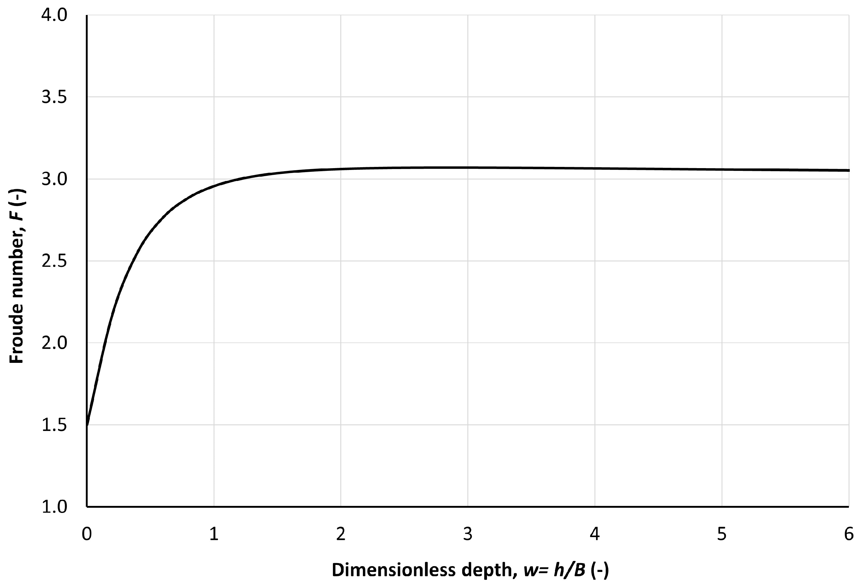
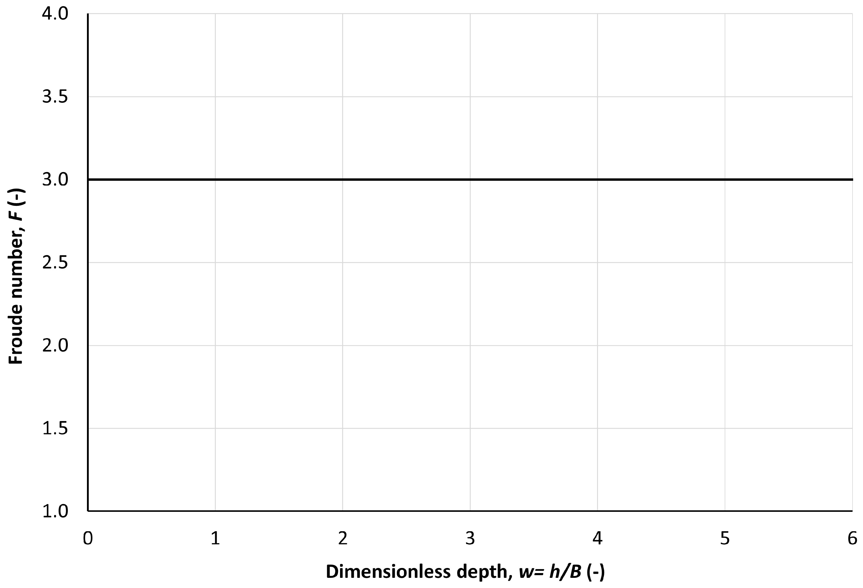
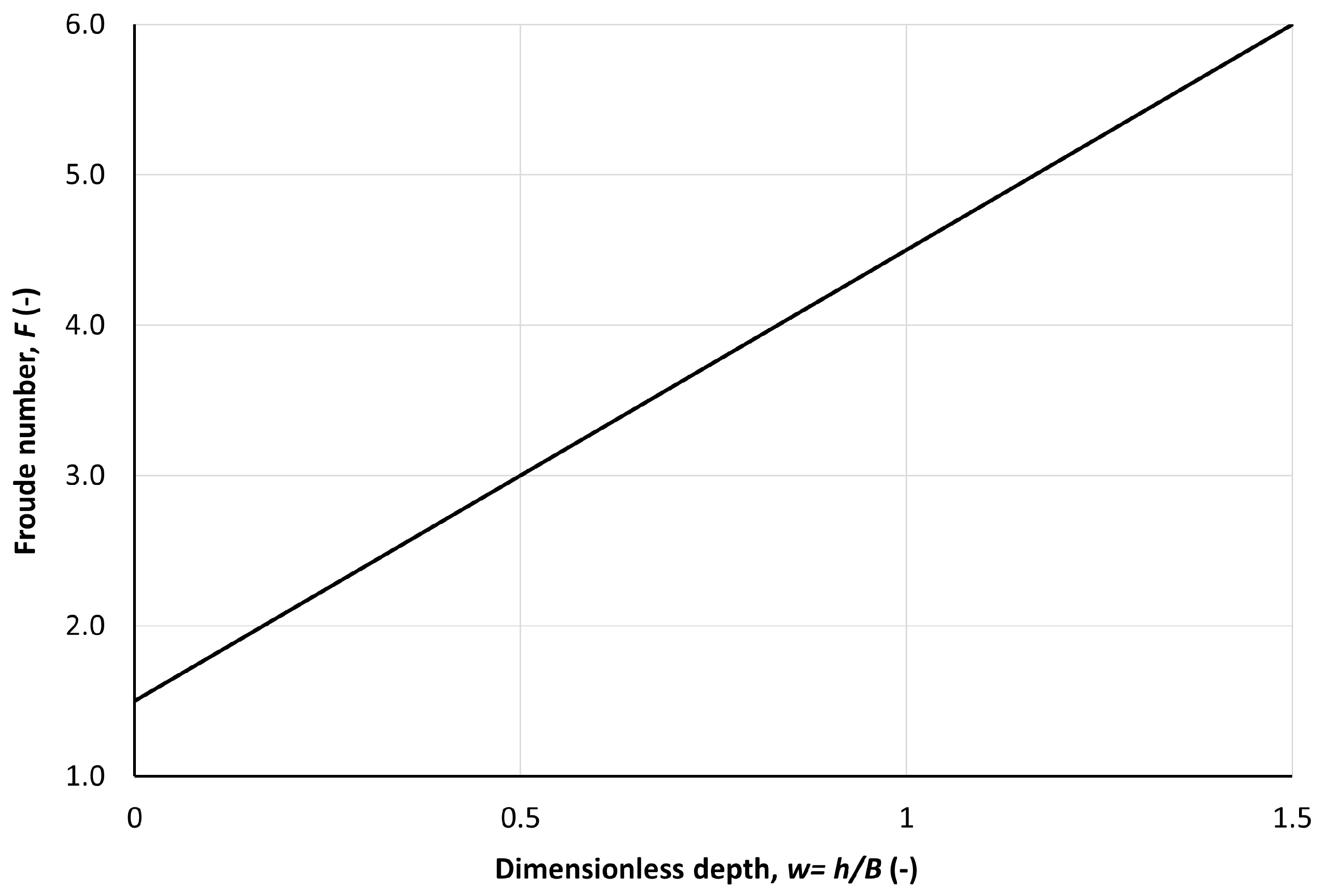
For a given prismatic channel, the maximum Froude number at which the 1D SWE remains solvable is determined by $F=\left|{\displaystyle \frac{rR}{mD}}{\displaystyle \frac{dh}{dR}}\right|$ regardless of the numerical method used. Specifically, for very wide channels, the 1D SWE remain valid for $F\le 1.5$, under the Manning equation for the friction slope, while the Chézy equation allows validity for $F\le 2$.

5.

Roll waves formation is revisited in this paper, and a complete procedure to solve the 1D SWE with roll waves formation is provided.

6.

The uniform flow is not possible when the ill-posedness condition is not met. This is an important result, as the design of channels with high slopes is based on uniform flow concept.

7.

Finally, the findings regarding the ill-posedness of the 1D SWE discussed in this paper will enhance the quality of open-channel flow education at both undergraduate and graduate levels, ultimately contributing to the development of well-trained professionals in the field. The Vedernikov number should be integrated into open-channel flow curricula alongside the Froude number.

References

1. Cullen, M.J.P. Analysis of the semi-geostrophic shallow water equations. Phys. D Nonlinear Phenom. 2008, 237, 1461–1465. [Google Scholar] [CrossRef]
2. Cozzolino, L.; Varra, G.; Cimorelli, L.; Della Morte, R. Mathematical and numerical modelling of rapid transients at partially lifted sluice gates. Adv. Water Resour. 2023, 181, 104562. [Google Scholar] [CrossRef]
3. Levermore, C.D.; Sammartino, M. A shallow water model with eddy viscosity for basins with varying bottom topography. Nonlinearity 2001, 14, 1493–1515. [Google Scholar] [CrossRef]
4. Majda, A.J. Vorticity and the mathematical theory of incompressible fluid flow. Commun. Pure Appl. Math. 1986, 39, S187–S220. [Google Scholar] [CrossRef]
5. Majda, A.J.; Bertozzi, A.L. Vorticity and Incompressible Flow; Cambridge texts in applied mathematics; Cambridge University Press: New York, NY, USA, 2002. [Google Scholar]
6. Minatti, l.; Faggioli, L. The exact Riemann Solver to the Shallow Water equations for natural channels with bottom steps. Comput. Fluids 2023, 254, 105789. [Google Scholar] [CrossRef]
7. Orenga, P. Un théorème d’existence de solutions d’un problème de shallow water. Arch. Ration. Mech. Anal. 1995, 130, 183–204. [Google Scholar] [CrossRef]
8. Pritchard, D.; Dickinson, L. The near-shore behaviour of shallow-water waves with localized initial conditions. J. Fluid Mech. 2007, 591, 413–436. [Google Scholar] [CrossRef]
9. Rakotoson, J.M.; Temam, R.; Tribbia, J. Remarks on the nonviscous shallow water equations. Indiana Univ. Math. J. 2008, 57, 2969–2998. [Google Scholar] [CrossRef]
10. Varra, G.; Pepe, V.; Cimorelli, L.; Della Morte, R.; Cozzolino, L. The exact solution to the Shallow water Equations Riemann problem at width jumps in rectangular channels. Adv. Water Resour. 2021, 55, 103993. [Google Scholar] [CrossRef]
11. Qionglei, C.; Changxing, M.; Zhang, Z. On the Well-Posedness for the Viscous Shallow Water Equations. SIAM J. Math. Anal. 2008, 40, 443–474. [Google Scholar] [CrossRef]
12. Preissmann, A. Propagation des Intumescences Dans les Canaux et Les Rivières; Congres de l’Association Française de Calcul: Grenoble, France, 1961; First Congress of the French Association for Computation, Grenoble; pp. 433–442. (In French) [Google Scholar]
13. Wu, W. Computational River Dynamics; Taylor & Francis: London, UK, 2008. [Google Scholar]
14. Popescu, I. Computational Hydraulics: Numerical Methods and Modeling; IWA Publishing: London, UK, 2014. [Google Scholar]
15. Meselhe, E.A.; Holly, F.M., Jr. Invalidity of Preissmann scheme for transcritical flow. J. Hydraul. Eng. 1997, 123, 652–655. [Google Scholar] [CrossRef]
16. Johnson, T.; Baines, M.J.; Sweby, P.K. A box scheme for transcritical flow. Int. J. Numer. Methods Eng. 2002, 55, 895–912. [Google Scholar] [CrossRef]
17. Freitag, M.A.; Morton, K.W. The Preissmann box scheme and its modification for transcritical flows. Int. J. Numer. Methods Eng. 2007, 70, 791–811. [Google Scholar] [CrossRef]
18. Sart, C.; Baume, J.P.; Malaterre, P.O.; Guinot, V. Adaptation of Preissmann’s scheme for transcritical open channel flows. J. Hydraul. Res. 2010, 48, 428–440. [Google Scholar] [CrossRef]
19. Samuels, P.G.; Skeels, C.P. Stability limits for Preissmann’s scheme. J. Hydraul. Eng. 1990, 116, 997–1012. [Google Scholar] [CrossRef]
20. Kutija, V.; Newett, C.J.M. Modelling of supercritical flow conditions revisited; NewC Scheme. J. Hydraul. Res. 2002, 40, 145–152. [Google Scholar] [CrossRef]
21. AlQasimi, E.; Mahdi, T.-F. A new one-dimensional numerical model for unsteady hydraulics of sediments in rivers. Discov. Appl. Sci. 2020, 2, 1480. [Google Scholar] [CrossRef]
22. Yu, C.-W.; Hodges, B.R.; Liu, F. A new form of the Saint-Venant equations for variable topography. Hydrol. Earth Syst. Sci. 2020, 24, 4001–4024. [Google Scholar] [CrossRef]
23. Fread, D.L.; Jin, M.; Lewis, J.M. An LPI Numerical Implicit Solution for Unsteady Mixed Flow Simulations. In Proceedings of the ASCE North American Water and Environment Congress, Anaheim, CA, USA, 22–28 June 1996. [Google Scholar]
24. Fread, D.L.; Lewis, J.M. FLDWAV: A generalized Flood Routing Model. In Proceedings of the National Conference on Hydraulic Engineering, ASCE, Colorado Springs, CO, USA, 8–12 August 1998; pp. 668–673. [Google Scholar]
25. DHI. MIKE 11—A Modelling System for Rivers and Channels; DHI—Water & Environment: Hørsholm, Denmark, 2004. [Google Scholar]
26. US Army Corps of Engineers. HEC-RAS River Analysis System, Hydraulic Reference Manual, Version 6.0.; Hydrologic Engineering Center: Davis, CA, USA, 2020; 518p.
27. Neumaier, A. Solving ill-conditioned and singular linear systems: A tutorial on regularization. SIAM Rev. 1998, 40, 636–666. [Google Scholar] [CrossRef]
28. Chow, V.T. Open-Channel Hydraulics; McGraw-Hill: New York, NY, USA, 1959. [Google Scholar]
29. Henderson, F.M. Open Channel Flow; MacMillian: New York, NY, USA, 1966. [Google Scholar]
30. Chaudhry, M.H. Open-Channel Flow, 2nd ed.; Springer: Berlin/Heidelberg, Germany, 2008; p. 523. [Google Scholar]
31. Liggett, J.A. Stability. Unsteady Flow in Open Channels, 1st ed.; Water Resources Publications: Fort Collins, CO, USA, 1975. [Google Scholar]
32. Cunge, J.A.; Holly Jr, F.M.; Verwey, A. Practical Aspects of Computational River Hydraulics; Pitman Publishing: Lanham, MD, USA, 1980. [Google Scholar]
33. Godounov, S.; Riabenki, V. Schémas Aux Différences (French); Editions Mir: Moscow, Russia, 1977; 361p. [Google Scholar]
34. Vedernikov, V.V. Characteristic Features of a Liquid Flow in an Open Channel, C.-R. (Doklady); Academy of Sciences of the USSR: Moscow, Russia, 1946; pp. 207–210. [Google Scholar]
35. Dooge, J.C.I. Linear Theory of Hydrologic Systems; United States Department of Agriculture: Washington, DC, USA, 1973. [Google Scholar]
36. Ponce, V.M.; Simons, B. Shallow Wave Propagation in Open Channel Flow. J. Hydraul. Div. 1977, 103, 1461–1476. [Google Scholar] [CrossRef]
37. Hadamard, J. Sur les Problèmes Aux Dérivées Partielles et Leur Signification Physique; Princeton University Bulletin: Princeton, NJ, USA, 1902; pp. 49–52. [Google Scholar]
38. Gustafsson, B.; Kreiss, H.-O.; Oliger, J. Time-Dependent Problems and Difference Methods, 2nd ed.; John Wiley & Sons: Hoboken, NJ, USA, 2013; Volume 123. [Google Scholar]
39. Bronshtein, I.N.; Semendyayev, K.A.; Musiol, G.; Muehlig, H. Handbook of Mathematics, 5th ed.; Springer: Berlin/Heidelberg, Germany, 2007; p. 1164. [Google Scholar]
40. Sturm, T.W. Open Channel Hydraulics; McGraw-Hill: New York, NY, USA, 2001. [Google Scholar]
41. Kvočka, D.; Ahmadian, R.; Falconer, R.A. Flood Inundation Modelling of Flash Floods in Steep River Basins and Catchments. Water 2017, 9, 705. [Google Scholar] [CrossRef]
42. Mingham, C.G.; Causon, D.M.; Ingram, D.; Mingham, C.G.; Causon, D.M.; Ingram, D. A TVD MacCormack scheme for transcritical flow. In Proceedings of the Institution of Civil Engineers—Water and Maritime Engineering; ICE Virtual Library (ICE Publishing): London, UK, 2001; Volume 148, pp. 167–175. [Google Scholar] [CrossRef]
43. Hirsch. Numerical Computation of Internal and External Flows. Vol.1: Fundamentals of Numerical Discretization; John Wiley: Chichester, UK, 1988. [Google Scholar]
44. Powell, R.W. Vedernikov’s criterion for ultra-rapid flow. Trans. Am. Geophys. Union 1948, 29, 882–886. [Google Scholar]
45. Chen, C. Free-Surface Stability Criterion as Affected by Velocity Distribution. J. Hydraul. Eng. 1995, 121, 736–743. [Google Scholar] [CrossRef]
46. French, R.H. Open-Channel Flow; McGraw-Hill, Inc.: New York, NY, USA, 1985; 551p. [Google Scholar]
Figure 1. Froude number threshold of ill-posedness for a trapezoidal channel of side slope z = 1, and bottom width B , using the Manning equation. Ill-posedness region is located above the curve.
Mathematics 13 02476 g001
Figure 2. Froude number threshold of ill-posedness for a triangular channel of any side slope z, using the Manning equation. Ill-posedness region is located above the curve.
Mathematics 13 02476 g002
Figure 3. Froude number threshold of ill-posedness for a rectangular channel of bottom width B , using the Manning equation. Ill-posedness region is located above the curve.
Mathematics 13 02476 g003
Disclaimer/Publisher’s Note: The statements, opinions and data contained in all publications are solely those of the individual author(s) and contributor(s) and not of MDPI and/or the editor(s). MDPI and/or the editor(s) disclaim responsibility for any injury to people or property resulting from any ideas, methods, instructions or products referred to in the content.