Prediction of China’s Silicon Wafer Price: A GA-PSO-BP Model

Abstract

The BP (Back-Propagation) neural network model (hereafter referred to as the BP model) often gets stuck in local optima when predicting China’s silicon wafer price, which hurts the accuracy of the forecasts. This study addresses the issue by enhancing the BP model. It integrates the principles of genetic algorithm (GA) with particle swarm optimization (PSO) to develop a new model called the GA-PSO-BP. This study also considers the material price from both the supply and demand sides of the photovoltaic industry. These prices are important factors in China’s silicon wafer price prediction. This research indicates that improving the BP model by integrating GA allows for a broader exploration of potential solution spaces. This approach helps to prevent local minima and identify the optimal solution. The BP model converges more quickly by using PSO for weight initialization. Additionally, the method by which particles share information decreases the probability of being confined to local optima. The upgraded GA-PSO-BP model demonstrates improved generalization capabilities and makes more accurate predictions. The MAE (Mean Absolute Error) value of the GA-PSO-BP model is 31.01% lower than those of the standalone BP model and also falls by 19.36% and 16.28% relative to the GA-BP and PSO-BP models, respectively. The smaller the value, the closer the prediction result of the model is to the actual value. This model has proven effective and superior in China’s silicon wafer price prediction. This capability makes it an essential resource for market analysis and decision-making within the silicon wafer industry.

1. Introduction

Many countries are responding to the global trend toward green and sustainable development. They are setting emission reduction targets and working to transform their energy consumption structures to low-carbon and cleaner alternatives. Due to rapid industrialization and urbanization, air pollution has become an increasing issue in China [1]. As the leading global consumer of energy and the top emitter of carbon, China holds a vital position in addressing worldwide pollution control [2,3,4]. The photovoltaic industry plays a key role in achieving low-carbon development. As a renewable clean energy source, it contributes significantly to sustainable energy goals [5]. Solar photovoltaic power has grown rapidly within China’s renewable energy generation system. The Chinese government is increasingly focused on the photovoltaic industry, establishing a series of policies to support its growth [6]. In this context, the silicon wafer is an essential raw material for the photovoltaic industry. Its price fluctuations directly affect the costs and competitiveness of solar products, significantly influencing the overall growth and direction of the industry. Therefore, accurately predicting China’s silicon wafer price is vital for ensuring the stability of the photovoltaic supply chain.

Recently, the application of deep learning has become extensively prevalent within the forecasting domain, focusing predominantly on three key areas. The first is housing price prediction. Deep learning networks have shown good performance in medium- to long-term housing price forecasts [7,8,9]. For instance, studies have shown that, when the BP model is applied to predict housing prices, its enhanced form outperforms conventional models regarding both accuracy and stability [10,11]. The second area is stock price prediction. Deep learning has demonstrated excellence in the collection and processing of stock data [12], as well as in stock price prediction [13]. Moreover, deep learning combines the advantages of different neural networks, making it superior to traditional single models and resulting in higher accuracy in stock price prediction [14,15,16,17]. The third area is energy price prediction. Deep learning has achieved significant progress in predicting electricity price and carbon price, with notable improvements in prediction accuracy compared to traditional algorithms [18,19,20,21]. Neural network training usually relies on gradient descent techniques, which can easily lead to problems such as local minima. Additionally, the BP neural network model faces issues like slow training times and reduced recognition accuracy [22,23,24]. Metaheuristic algorithms, such as Genetic Algorithm (GA), Particle Swarm Optimization (PSO), Ant Colony Algorithm (ACO), etc., do not rely on gradient information and can search globally, helping to find more globally optimal solutions and avoiding getting stuck in local minima. The main purpose of combining metaheuristic algorithms with neural networks is to address the shortcomings of conventional optimization methods and to improve the global search capability [25,26,27,28]. This prompts us to explore the potential of hybrid models combining GA and PSO to improve the BP model and accurately predict China’s silicon wafer price.

Many studies have verified the effectiveness of metaheuristic algorithms in estimation and prediction. Scholars have used GA to optimize BP model parameters [29,30] and PSO to accelerate convergence [31,32], enhancing both performance and prediction accuracy. Their findings indicated that the optimized models outperformed the conventional BP model concerning overall risk assessment and the precision of risk categorization. However, GA faces challenges such as slow initial search efficiency, prolonged training times, and limited local search precision, which hinder thorough model optimization [33]. The PSO algorithm tends to converge prematurely and may get trapped in local optima. As a result, researchers frequently focus on enhancing these methods by modifying or refining existing optimization algorithms [34]. The GA-PSO-BP model effectively combines the global search power of GA with the local search efficiency of PSO. By integrating both global and local optimization, this hybrid approach enhances model accuracy and accelerates the training process. The GA-PSO-BP model effectively addresses the issues of inadequate optimization or slow convergence that can occur with using a single method, making it more efficient for tackling complex prediction tasks [35]. The GA-PSO-BP model has demonstrated its effectiveness in complex prediction tasks, achieving strong results in areas such as photovoltaic power generation [36], medical diagnosis [37], sensor network positioning [38], carbon price forecasting [39], and seal leakage rate prediction [40]. Inspired by existing studies, this study seeks to create a GA-PSO-BP model to forecast China’s silicon wafer price, contributing to the advancement of research in this area. This study compares the GA-PSO-BP model with the GA-BP model and PSO-BP model, and the results show that the upgraded GA-PSO-BP model is optimized in terms of MAE, RMSE, and R² performance. Specifics will be presented in the main text.

Based on the above, this study utilized the BP model and combined the GA and PSO algorithms to construct the GA-PSO-BP model to improve its performance. Three error metrics are utilized to evaluate the advantages and disadvantages of GA-BP, PSO-BP, and GA-PSO-BP in exploring the prediction of China’s silicon wafer price. The innovations of this study and the knowledge gaps it fills are as follows. (1) Previous scholars often used the GA-BP or PSO-BP individually for price prediction. They did not combine the two models in their analyses. This limited the optimization capability of the models. We construct the GA-PSO-BP model in this study to predict China’s silicon wafer price. This model enhances optimization ability by combining both algorithms. (2) Past research has primarily focused on using GA and PSO for applications of housing price prediction and risk assessment. However, there has been limited focus on China’s silicon wafer price prediction. Silicon wafers are crucial in the photovoltaic industry, and their prices are influenced by multiple factors. The GA-PSO-BP model is capable of conducting a thorough analysis and optimization of these factors comprehensively. This approach improves the accuracy of China’s silicon wafer price prediction and offers a scientific foundation for strategic decision-making within the photovoltaic sector. (3) Most prior research in the photovoltaic industry has concentrated on the development status and trends of photovoltaic technology. However, there has been limited focus on the prices of specific components within the photovoltaic industry chain. This study fills this gap by specifically focusing on China’s silicon wafer price prediction, which significantly influences the cost framework of photovoltaic systems.

The organization of this study is structured as follows. Section 2 introduces the operating mechanisms of the three types of neural networks. Section 3 develops a predictive model for China’s silicon wafer prices using the GA-PSO-BP model and performs experiments and analysis utilizing MATLAB R2023b. Finally, we present the conclusions of this study.

2. Construction of the GA-PSO-BP Model

2.1. BP Model

The BP model constitutes a feedforward architecture that employs the method of error backpropagation. It simulates the connections and information transmission processes found in human brain neurons. By employing a backpropagation algorithm, the model can learn and achieve complex nonlinear mappings of input data. Figure 1 illustrates that the BP model usually comprises three layers. Throughout the training phase, the system establishes mapping from the input data to the intended output. It repeatedly adjusts the weights and biases within the network to reduce prediction errors.

The BP model’s learning procedure consists of two key phases: forward and backward propagation. During the forward propagation process, the hidden layer receives input data from the input layer, sequentially processes this information, and then forwards the outcomes to the output layer. When the output layer’s result differs from the expected target, the network enters the backpropagation phase. This indicates that the error signal propagates in the reverse direction, starting from the output layer and moving towards the input layer. During this process, the algorithm adjusts the weights between layers to gradually reduce the error. Essentially, the algorithm trains the model through repeated iterations and guides the error function to move in the most efficient direction to minimize error. This process allows the network to settle at a point of minimum error. Once this point is reached, training is complete, and the network retains its best version. Within the BP model, the sigmoid activation function is typically used in the hidden layer, which is mathematically expressed as follows:

$$S=1/(1+e^{(-x)})$$

(1)

where $e$ is the base of the natural logarithm and $x$ is the weighted input of the previous layer.

In the BP model, the loss function commonly used is the Mean Squared Error (MSE), which measures the difference between the predicted results and the true values. The lower the MSE, the closer the model’s forecasted results are to the true values. This signifies that the model performs better. The MSE loss function is as follows:

$$MSE={\displaystyle \frac{1}{K}}{\displaystyle \sum _{i=1}^K{(y_i-o_i)}^2}$$

(2)

where $K$ means the total count of samples, ${\mathrm{y}}_i$ refers to the actual value for the i-th sample, $o_i$ represents the predicted value for the i-th sample, and $(y_i-o_i)$ denotes the difference between the predicted value and the actual outcomes.

The BP model has strong nonlinear processing capabilities. This allows it to solve complex nonlinear problems and makes it useful in various prediction applications. Additionally, the BP model can learn from a set of instances with target solutions. This ability to automatically extract “reasonable” solutions demonstrates its self-learning capabilities [41,42]. Nevertheless, the BP model faces certain challenges. The model tends to get trapped in local minima, which results in a slower convergence process [10]. Therefore, to address these problems, this study employs GA and PSO to enhance the BP model.

2.2. GA-PSO Algorithm

2.2.1. GA-BP Model

The GA is used to solve optimization problems by simulating the mechanism of natural selection. The GA improves candidate solutions through iterative processes, using mechanisms like selection, crossover, and mutation. Typically, the starting population of the GA is generated at random. This maintains variety within the population and prevents the initial solution from concentrating in a specific region, thereby enhancing the algorithm’s global search capability. Throughout this iterative process, individuals’ fitness within the population is assessed and compared. This incremental exploration seeks to identify the most favorable outcome by the principle of natural selection. As a result, a new population of solutions emerges, representing the best options for the problem at hand. Scholars have employed GA to refine the weights and thresholds within neural networks. Such a combination enhances the networks’ capacity for generalization and efficient convergence [43,44]. By integrating the GA with the BP model, we enhance the BP model’s capabilities, especially for dealing with high-dimensional, non-linear, or intricate issues. The GA assists the BP model in avoiding local minima and discovering globally optimal solutions. The GA-BP model has been widely implemented in sectors like transportation and energy [45,46].

The steps for optimizing the BP model with the GA are described below. This procedure includes specific methods for fine-tuning the model.

(1) Initialization: The entire population is initialized by generating N individuals using parameter encoding. These individuals are randomly generated within a defined range for each parameter, which ensures diversity in the population. The N individuals constitute the initial population. The size of this population is then used to assess chromosome length and range, along with defining a target error value.

(2) Fitness Calculation: The fitness $f$ is calculated using the formula below.

$$\left\{\begin{array}{c}f={\displaystyle \frac{1}{SE}}\\ SE={\displaystyle \sum {(y_i-o_i)}^2}\end{array}\right.$$

(3)

where ${\mathrm{y}}_i$ represents the network’s expected value, $o_i$ denotes the obtained value, and $SE$ represents the function of the squared error sum.

(3) Selection: Select individuals with higher fitness values based on survival-of-the-fittest principles. Common selection methods include roulette wheel selection and tournament selection.

(4) Crossover: Selecting the k-th position chromosome $a_k$ and the i-th position chromosome $a_i$, the cross-operation method at the j-th position is detailed below, and ${a^{\prime }}_k$ and ${a^{\prime }}_i$ are the new individuals resulting from the crossover:

$$\left\{\begin{array}{c}{a^{\prime }}_k=a_k(1-b)+a_{i}b\\ {a^{\prime }}_i=a_i(1-b)+a_{k}b\end{array}\right.$$

(4)

where $b$ means the weighting factor, $b\in [0,1]$.

(5) The mutation operation for the i-th individual at the j-th gene is expressed by the following formula:

$$aij=\left\{\begin{array}{c}{a}_{ij}+(a_{ij}-a_{\max })f(g),rand()\ge 0.5\\ a_{ij}+(a_{\min }-a_{ij})f(g),rand()<0.5\end{array}\right.$$

(5)

where $a_{\max }$ and $a_{\min }$ represent the lower and upper bounds of the chromosome $a_{ij}$, respectively. $f(g)=(1-g/G_{\max })rand()$; $g$ signifies the present iteration count, while $G_{\max }$ indicates the upper limit of evolutionary iterations, and $rand()\in [0,1]$ means a random number.

(6) Evaluation and Termination: Assess the fitness of each individual in the population and determine the error. Check whether the termination criteria are satisfied. If they are, move on to step (7); if not, go back to step (3).

(7) Optimal Weight and Threshold: Establish the most effective weight and threshold parameters for the BP model.

(8) Correction: Fine-tune the parameters (weights and biases) at each layer of the BP model.

(9) Error Calculation: Determine the discrepancy within the BP model. If the error is within the required range, terminate the entire process; otherwise, return to step (7) to continue correcting the network parameters.

(10) Data Saving: Obtain the optimized data and save the network space and mapping relationships.

2.2.2. PSO-BP Model

The PSO is based on foraging behavior observed in bird flocks. It is an optimization approach that relies on a population. In this algorithm, each “particle” signifies a potential solution. These particles navigate the search space, adjusting their positions and velocities. They achieve this by keeping track of their personal best positions, along with the best position discovered by the whole group. The PSO can optimize the weight initialization and structural parameters of a BP model. Applying PSO to initialize the parameters of the BP model can enhance the network’s convergence rate and decrease the likelihood of it getting trapped in local optima. It is particularly effective in training neural networks, enhancing both their performance and generalization capabilities.

During the PSO iteration process, each particle modifies its position according to its present velocity. It also evaluates its performance using the fitness function. The particles modify their positions and speeds according to their optimal solutions and the best solution found by the entire swarm. gbest (Global Best) refers to the optimal solution encountered by all particles in PSO, while pbest (Particle Best) refers to the optimal solution encountered by a single particle in PSO. Equations (6) and (7) provide the formulas used to update the particle’s velocity and position:

$$v_{i,j}(t+1)=w{v}_{i,j}(t)+c_1(pbes{t}_{i,j}(t)-x_{i,j}(t))rand()+c_2(gbest(t)-x_{i,j}(t))rand()$$

(6)

$$x_{i,j}(t+1)=x_{i,j}(t)+v_{i,j}(t+1)$$

(7)

where $v_{i,j}(t+1)$ represents the velocity of the i-th particle in the j-th dimension at the (t + 1)-th iteration, $w$ represents the inertia weight, which is employed to balance exploration and exploitation and is commonly calculated using the Formula (8) [47], and $v_{i,j}(t)$ is the velocity of the i-th particle in the j-th dimension at the t-th generation. $c_1$ and $c_2$ are the cognitive and social acceleration constants, generally $c_1=c_2=2$; $rand()$ means random values ranging from 0 to 1; $pbes{t}_{i,j}(t)$ is the particle best position of the i-th particle in the j-th dimension at the t-th iteration; $gbest(t)$ represents the global best position on the j-th dimension at the t-th iteration; $x_{i,j}(t+1)$ refers to the position of the i-th particle in the j-th dimension at the (t + 1)-th iteration; and $x_{i,j}(t)$ means the position of the i-th particle in the j-th dimension at the t-th iteration.

$$w={\displaystyle \frac{0.5+rand()}{2}}$$

(8)

where $rand()$ is a randomly generated number.

2.2.3. GA-PSO-BP Model

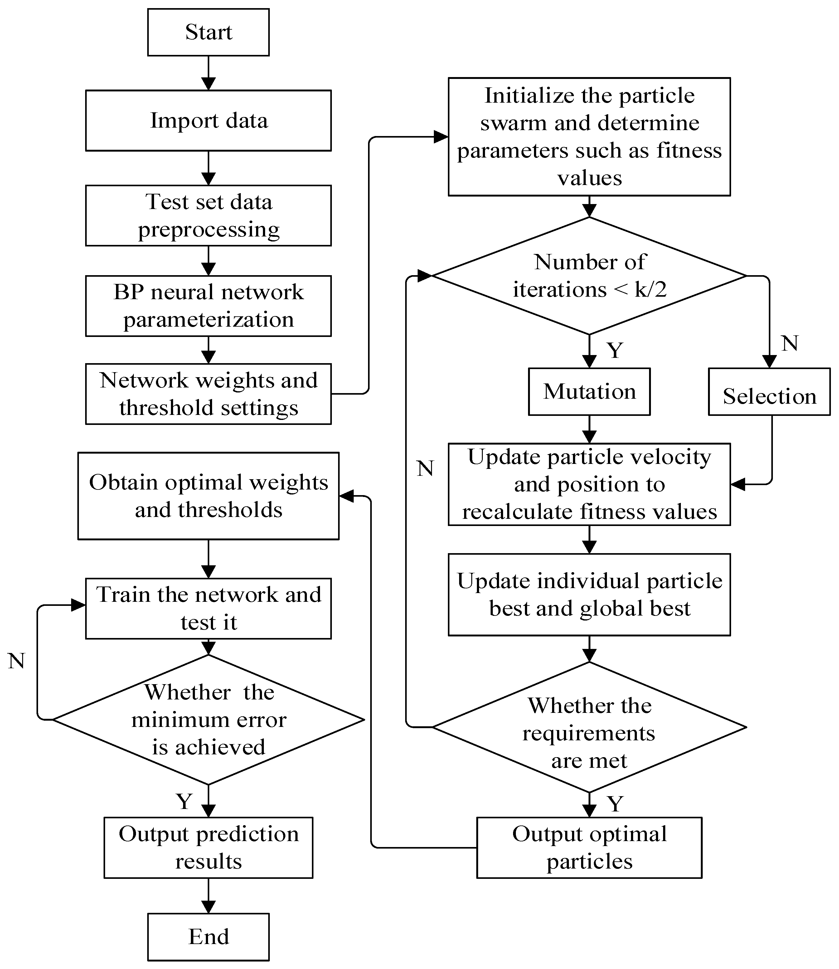
The GA-PSO-BP model combines the strengths of GA, PSO, and the BP model. This combination creates an advanced hybrid optimization algorithm (Figure 2). The initial population of the GA-PSO-BP model is randomly generated. First, the model takes advantage of the global exploration capability of the GA to modify the starting weights and biases in the BP model. This optimization expands the solution space available to the BP model during its initial training phase. Next, the PSO refines the adjustments of weights and biases. It mimics the foraging behavior of bird flocks to improve the BP model’s local search performance. Finally, the BP model refines its weights and biases iteratively to minimize prediction errors. The GA-PSO-BP model mimics the maturation process found in nature. It applies the PSO to further enhance the best solutions identified in each generation of the genetic algorithm, aiming for improved optimization results. This hybrid optimization strategy improves the BP model’s prediction accuracy while also boosting its generalization ability in complex tasks. As a result, it performs exceptionally well in nonlinear function fitting, data classification, and time series prediction. In Figure 2, the structural diagram of the GA-PSO-BP model is demonstrated.

The formulas are detailed below:

$$pbes{t}_i=\left\{\begin{array}{l}pbes{t}_i,iff(pbes{t}_i)\le f(x_i)\hfill \\ x_i,otherwise\hfill \end{array}\right.$$

(9)

where $pbes{t}_i$ represents the best position found by $i$, $x_i$ denotes the current position of $i$, and $f$ is the fitness function.

$$gbest=\left\{\begin{array}{l}gbest,iff(gbest)\le f(pbes{t}_i)\hfill \\ pbes{t}_i,otherwise\hfill \end{array}\right.$$

(10)

where $gbest$ represents the best position found across the swarm.

3. China’s Silicon Wafer Price Prediction Based on the GA-PSO-BP Model

3.1. Data Collection

Silicon wafers are a crucial material in semiconductor production, and their price variations greatly influence the overall photovoltaic supply chain in China. This study aims to develop an accurate prediction model by analyzing various factors that influence China’s silicon wafer price. According to relevant studies, activities within the distributed photovoltaic industry chain are categorized into three stages: upstream, midstream, and downstream. Silicon wafer prices, which play a crucial role in the photovoltaic supply chain, are significantly affected by the demand from both upstream and downstream sectors [48,49]. To accurately predict the price of silicon wafers, this study selects seven key indicators to predict China’s silicon wafer price, using data from 21 April 2023 to 18 June 2024.

Table 1. Statistics of selected influencing factors.

Index	Polycrystalline Silicon Dense Material Price (10,000 Yuan Per Ton)	Aluminum Alloy Price (USD Per Ton)	Chip Price (Index Point)	Battery Cell Price (Yuan Per Piece)	Thin-Film Photovoltaic Modules Price (USD Per Watt)	Tempered Glass Price (Yuan Per Square Meter)	New Installed Capacity of Photovoltaics (Million Kilowatts)
Beginning date	21 April 2024	21 April 2024	21 April 2024	21 April 2024	21 April 2024	21 April 2024	21 April 2024
End date	18 June 2024	18 June 2024	18 June 2024	18 June 2024	18 June 2024	18 June 2024	18 June 2024
Mean	7.36	1753.99	94.41	0.59	0.71	52.72	10,409.33
Median	6.56	1730.26	94.77	0.51	0.70	52.57	8294.61
Variance	11.84	56,704.74	127.64	0.07	0.01	39.16	45,880,469.49
Standard deviation	3.44	238.13	11.30	0.26	0.08	6.26	6773.51
Max	22.01	2320.71	114.11	1.33	0.85	63.42	25,867.66
Min	3.01	1218.84	76.40	0.26	0.57	42.35	2741.45

shows the descriptive statistics for the selected data, while

Table 2. Data sources.

Index	Indicator Variable	Data Sources
Raw material prices	Polycrystalline silicon dense material price	Antaike
	Aluminum alloy price	Ministry of commerce
Prices of related product	Chip price	China Huaqiangbei Electronic Market Price Index Website
	Battery cell price	PV InfoLink
Indicators of photovoltaic industry	Thin-film photovoltaic modules price	Energy Trend
	Tempered glass price	Choice Data
	New installed capacity of photovoltaics	National Energy Administration

details the data sources.

3.1.1. Polycrystalline Silicon Dense Material Price

Silicon wafers are direct downstream products of polysilicon. The cost of producing silicon wafers consists of the price of several components: silicon material consumption, electricity usage, equipment depreciation, and water consumption. Among these components, silicon material consumption represents the largest portion. As a result, changes in silicon prices have a direct impact on the manufacturing expenses of silicon wafers. Polysilicon prices can be a critical indicator for measuring changes in silicon wafer production costs. If the price of polysilicon rises, it will lead to an increase in the production costs of silicon wafers. This increase may also trigger adjustments in the market price of silicon wafers.

3.1.2. Aluminum Alloy Price

Aluminum alloy is commonly used for structural components, such as photovoltaic mounting systems. If the price of aluminum alloy increases, it may raise the overall cost of photovoltaic systems. This increase can indirectly affect the demand and price of silicon wafers. According to the cost pass-through effect, a rise in aluminum alloy prices leads to higher production costs for PV mounting systems. This, in turn, can increase the overall costs of photovoltaic systems. Under this cost pressure, photovoltaic module manufacturers may look for ways to reduce other expenses, including the cost of silicon wafers.

3.1.3. Chip Price

The growth in market demand for chips will directly increase the demand for silicon wafers, as they are a key downstream application. The market forces of supply and demand within the chip market will have an impact on the pricing of silicon wafers. If there is a shortage of chips, manufacturers may respond by increasing production. This rise in production will boost the demand for silicon wafers, potentially driving up their price.

3.1.4. Battery Cell Price

In recent years, many battery cell manufacturing companies have adopted a vertically integrated production model. This model includes the production of silicon wafers, battery cells, and modules. Companies are progressively extending their operations in both directions along the supply chain. Battery cell production is typically in line with that of downstream modules. Since battery cells are a direct downstream product of silicon wafers, their price fluctuations can impact the demand for and pricing of silicon wafers. When the price of battery cells increases, it may create cost pressure for photovoltaic module manufacturers. This pressure could prompt them to reevaluate their raw material costs, including silicon wafer prices. If the cost pressure becomes too high, manufacturers may look for more affordable sources of silicon wafers or reduce their usage. Additionally, fluctuations in battery cell prices will influence the supply chain management strategies of photovoltaic module manufacturers. They may adjust their procurement plans for silicon wafers based on changes in battery cell prices.

3.1.5. Thin-Film Photovoltaic Modules Price

According to the annual report from the China Photovoltaic Industry Association, global module capacity and output reached 1103 GW and 612.2 GW, respectively, by the end of 2023. These figures represent year-on-year increases of 61.6% and 76.2%, respectively, indicating rapid growth in the industry. Photovoltaic modules are essential components of photovoltaic power plants. Thin-film photovoltaic modules serve as alternatives to silicon-based modules and compete with them in terms of price and performance. A reduction in the cost of thin-film solar panels could lead to a decrease in demand for silicon wafers. This change could affect China’s silicon wafer price. However, the impact on prices may also depend on factors such as technological efficiency and market acceptance.

3.1.6. Tempered Glass Price

Tempered glass and silicon wafers are parts of different segments of the photovoltaic industry chain. However, their price fluctuations can interact through various mechanisms. Strengthened glass is essential in photovoltaic modules. An increase in its price could elevate the total expenses for photovoltaic modules. This rise in cost may lead manufacturers to seek cost-control measures. They might reduce their demand for silicon wafers or consider alternative materials. These actions could ultimately affect China’s silicon wafer price.

3.1.7. Newly Installed Capacity of Photovoltaics

The newly installed capacity of photovoltaics is an important indicator of demand in the photovoltaic market. It directly affects China’s silicon wafer price. When newly installed photovoltaic capacity increases, this indicates a rising demand for photovoltaic modules. This, in turn, boosts the demand for silicon wafers. If the demand for silicon wafers grows, but the supply cannot keep up, then China’s silicon wafer price may rise. This relationship between supply and demand is a fundamental driving force behind price fluctuations in a market economy.

In summary, the various factors considered cover key dimensions such as raw material costs, intermediate product pricing, and final product demand. Together, these factors provide a strong foundation for analyzing China’s silicon wafer price. These factors are interconnected and create a complex network of interactions. For example, an increase in raw material costs can raise the production costs for intermediate goods. This, in turn, affects the pricing of final products and influences market supply and demand relationships. This chain reaction clearly illustrates the close connections between the factors at each stage of forming China’s silicon wafer price and their overall impact.

3.2. Data Preprocessing

Data normalization is a crucial step before using the GA-PSO-BP model to predict China’s silicon wafer price. This process ensures that features with a large numerical range do not have a disproportionate impact on model training, thereby improving the prediction accuracy of the model. In this study, the mapminmax function was used to standardize the data of the training and testing datasets, adjusting the values to fit the [0, 1] interval.

$$y=(y_{\max }-y_{\min }){\displaystyle \frac{x-x_{\min }}{x_{\max }-x_{\min }}}+y_{\min }$$

(11)

where $x$ is the original data, $x_{\min }$ and $x_{\max }$ are the minimum and maximum values of the original data, respectively, and $y_{\min }$ and $y_{\max }$ are the minimum and maximum values of the target range, respectively.

3.3. Model Construction and Parameter Settings

In the GA-PSO-BP model, this study uses an output model with one input layer, which consists of seven input variables, each corresponding to one of the seven factors influencing silicon wafer prices, five hidden layers, and one output layer to predict silicon wafer prices. The dataset includes daily data for 300 working days, which will be apportioned between a training dataset and a testing dataset in a proportion of 4:1. In total, 80% is designated for training, and the leftover 20% is used for testing. This division aims to provide reliable support for China’s silicon wafer price prediction. Throughout the training phase, GA and PSO were applied to fine-tune the BP model, allowing it to achieve optimal weights and thresholds, which in turn improved the model’s accuracy. In the final step, an error analysis was performed by comparing the predicted results with the actual outcomes. We use MATLAB as the simulation environment. The learning rate is fixed at 0.01. The training process aims for a target error of 10⁻⁴, and the maximum iteration count is 60,000.

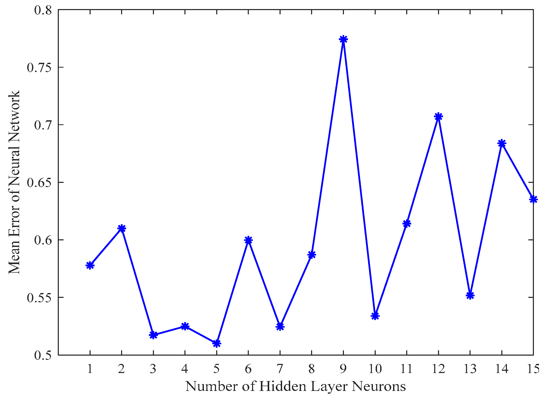
The configuration of hidden layers can help the network achieve a certain level of robustness to noise in the input data. By learning the useful information from the data, the network can to some extent ignore or suppress the impact of noise. To determine the optimal number of hidden layers for the BP model, multiple experiments were conducted in this study. This study compares the impact of different numbers of hidden layers on model performance. Figure 3 shows that, when there are five hidden layers, the predictive performance of the model is at its peak. This result is based on systematic testing of multiple hidden layer settings (from 1 to 15), each of which has been thoroughly trained and evaluated on the same training and testing datasets. Therefore, we conclude that setting the number of hidden layers in the BP model to five is the optimal choice in this study.

4. Experimental Results and Analysis

4.1. Simulation Results for the Model

The GA-PSO-BP model is utilized for China’s silicon wafer price prediction. The fitness curve demonstrates how individual or particle fitness values fluctuate as the optimization steps increase. In the context of GA and PSO, “optimal adaptation” typically refers to the fitness level of the best solution identified so far. In PSO, this may be the gbest. However, in GA, the optimal solution may be the individual exhibiting the best fitness within the current population. In this study, both GA and PSO are used in the model, so “optimal adaptation” refers to the better solution of the two algorithms. “Average adaptation” is the average adaptation of a population or swarm of particles that combines GA and PSO. Figure 4 shows the fitness curve for the GA-PSO-BP model.

Figure 4 displays how fitness values change with each iteration. During the iteration process, the algorithm slowly converges, and the fitness indicators start to stabilize. The two lines in Figure 4 are very close together. This proximity indicates that the algorithm finds solutions near the optimal solution, demonstrating good stability. The fitness indicators demonstrate a slight decrease as the iterations increase. This decline may occur because the algorithm is approaching the convergence point, where there is less room for further improvement.

In Figure 5, R represents the correlation coefficient. This coefficient, ranging from −1 to 1, evaluates how closely two variables are linearly related. The R value of approximately 0.93, nearing 1, signifies a robust positive correlation between the data points and the regression line. This suggests that, as the independent variable increases, the dependent variable tends to increase as well. According to Figure 5, the model demonstrates high prediction accuracy and is proficient at identifying linear relationships between data points.

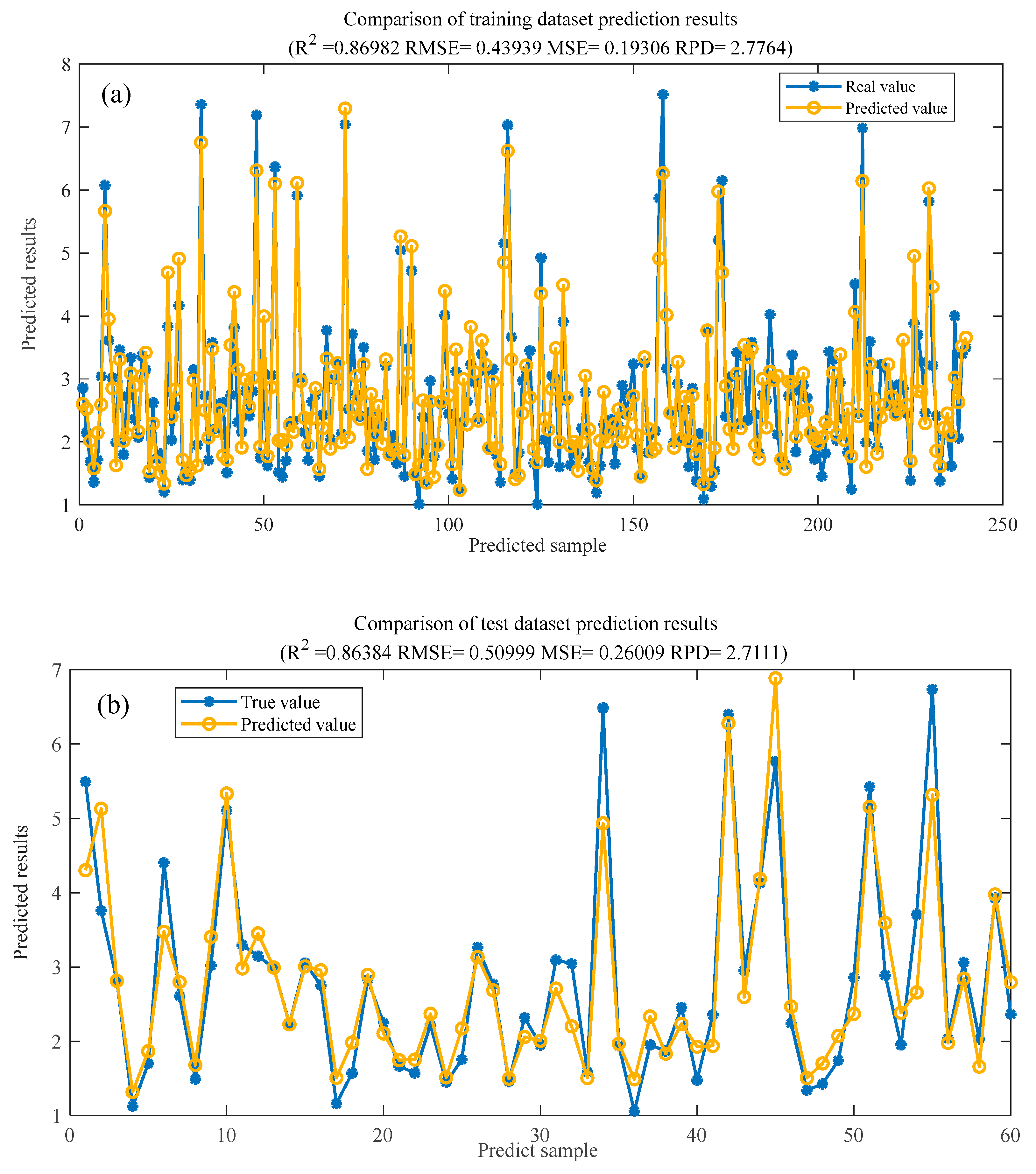
Next, 240 data points were selected as the training set. In Figure 6a, R² (coefficient of determination) is a measure of how accurately the model represents the data. The R² value of 0.86982, which is near 1, suggests a strong fit. RMSE (Root Mean Square Error) calculates the discrepancy between the predicted figures and the actual data. The RMSE value is 0.43939, and a smaller RMSE indicates more accurate predictions. MSE denotes the mean of the squared prediction errors, which is 0.19306. This value is the square of the RMSE. RPD (Relative Prediction Deviation), a metric for gauging the accuracy of predictive models, represents the relative deviation between predicted and actual values. Its value is 2.7764. A ratio greater than 1 typically indicates that the predicted results are acceptable. The formula for calculating RPD is as follows:

$$RPD={\displaystyle \frac{{\sigma }_{actual}}{RMSE}}$$

(12)

In Figure 6b, the model performs relatively accurately on the test dataset. The R² value of approximately 0.86 suggests that the model effectively captures the majority of the variation in the data. The values of RMSE and MSE provide a quantitative measure of prediction error. The magnitude of these values can help assess the model’s predictive accuracy. Although the RMSE value is slightly higher than that on the training dataset, it remains within an acceptable range. The RPD value is greater than 1, indicating that the predicted results are acceptable.

Figure 6 illustrates that the training and test sets display comparable errors, suggesting that the model generalizes well. Moreover, the error distribution is relatively uniform when predicting different samples, with no systemic bias present. The RPD values are consistent across both the training and test sets. This consistency suggests that the model performs stably across different datasets, with no signs of overfitting or underfitting.

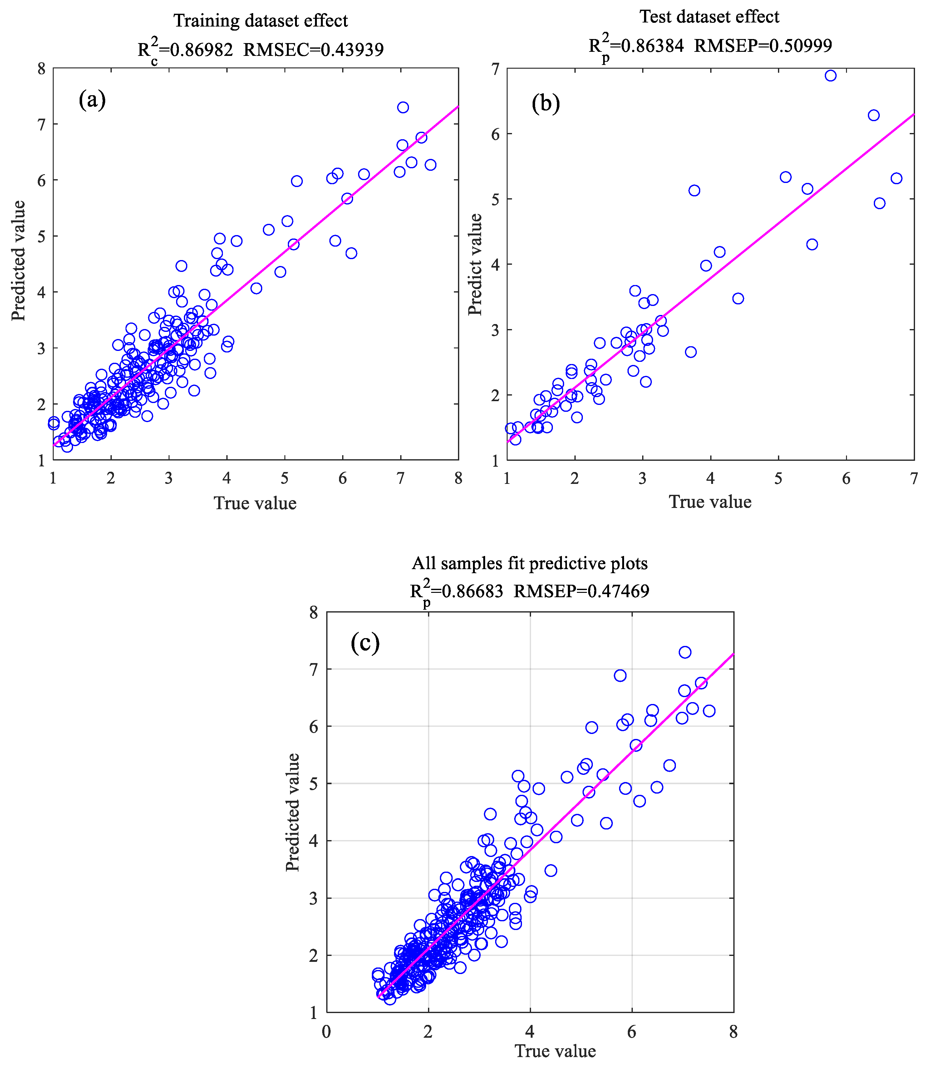
According to Figure 7, the GA-PSO-BP model exhibits a strong correlation with the training dataset, as well as the test dataset. Figure 7a shows the linear fitting of the model to the training dataset, with an R² of 0.86982. This value reflects a high degree of correlation and a substantial linear relationship between the predicted and observed values. The RMSE is 0.43939, which is a relatively low error value, meaning a small deviation in the predicted values compared to the actual values. Figure 7b displays how well the model performs on the test dataset, with a correlation coefficient R² of 0.86384, slightly lower than that of the training dataset, but still showing a strong correlation. The RMSEP is 0.50999, which is somewhat higher than the error for the training dataset. RMSEP (Root Mean Square Error of Prediction) is a metric used to evaluate the accuracy of a model’s predictions. It is calculated by taking the square root of the average of the squared differences between the predicted and actual values. This value reflects how close the predictions are to the actual outcomes, with a lower RMSEP value indicating better prediction accuracy. A smaller RMSEP value indicates better prediction accuracy. This implies a slight decrease in the model’s performance for previously unencountered data, while maintaining good predictive strength. Figure 7c presents the fitting prediction graph for all samples, with an R² of 0.86683, falling between the coefficients of the training and test datasets, indicating the model’s stability across the overall dataset. The RMSEP is 0.47469, which lies between the training and test errors, further demonstrating the model’s generalization ability.

A comprehensive analysis of Figure 7 reveals that the model performs excellently during the training phase, demonstrating high predictive accuracy. In the testing phase, the model maintains high correlation and low error, indicating good generalization ability. The fitting prediction graph for all samples further confirms the model’s stability and reliability across the overall dataset. The findings point to the GA-PSO-BP model being a valuable tool for China’s silicon wafer price prediction analysis.

4.2. Model Validation

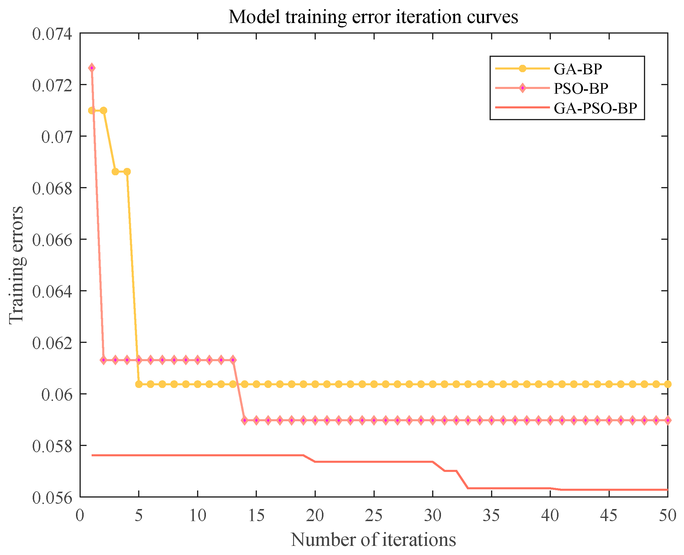
This study evaluates the predictive performance of the proposed GA-PSO-BP model. We conduct simulations and error analyses to compare the GA-PSO-BP model with the more traditional GA-BP and PSO-BP models. Figure 8 illustrates the performance of these three models across multiple iterations. The results show that the performance of the algorithms varies throughout the iterative process. Specifically, the GA-PSO-BP model achieves the best convergence speed and stability, outperforming the other two algorithms.

The GA-BP model shows rapid error reduction in the initial iterations, indicating a strong learning ability in the early stages. However, with an increasing number of iterations, the error reduction rate diminishes. This deceleration suggests that the GA-BP model may encounter local optima or other convergence challenges, leading to diminishing improvement in error reduction in later iterations.

The error reduction pattern in the PSO-BP model follows a trend similar to that of the GA-BP model. However, the PSO-BP model demonstrates slightly poorer performance at certain iteration stages. This could imply limitations in its capacity to effectively conduct global or local searches while striving to identify the optimal solution.

In contrast, the GA-PSO-BP model demonstrates more stable and smoother convergence throughout the entire process. This suggests that the hybrid model effectively balances the global search of GA and the local optimization of PSO, enabling it to consistently achieve lower errors with greater stability across iterations. Although the initial error may be lower, the model continues to optimize and reduce error throughout training. This balanced and stable convergence makes the GA-PSO-BP model particularly well-suited for complex tasks, as it avoids the fluctuations seen in other models and maintains consistent performance over time.

Meanwhile, to more accurately evaluate the predictive performance of each model, this study uses three metrics, RMSE, MAE, and R², to evaluate the precision of the models’ predictions [50]. The MAE (Mean Absolute Error) quantifies the average magnitude of prediction errors, and it is widely used to evaluate the accuracy of predictions. These metrics are selected for their ability to capture different aspects of prediction accuracy, which offer a balanced and in-depth analysis of the models’ predictive capabilities.

Table 3. Evaluation of prediction results.

MODEL	MAE	RMSE	R2
BP	0.51125	0.66847	0.7571
GA-BP	0.43725	0.56015	0.84374
PSO-BP	0.42117	0.59387	0.81536
GA-PSO-BP	0.3526	0.50999	0.86384

presents the detailed information.

Table 3 presents a comparative evaluation of prediction performance across four models, BP, GA-BP, PSO-BP, and GA-PSO-BP, using MAE, RMSE, and R² as the evaluation metrics. The standard BP model exhibits the weakest performance, with the highest MAE (0.51125) and RMSE (0.66847) and the lowest R² value (0.7571), indicating limited accuracy and poor generalization. The introduction of metaheuristic optimization significantly improves prediction performance. The GA-BP and PSO-BP models both reduce prediction errors compared to BP, with PSO-BP achieving a slightly lower MAE (0.42117) and a slightly lower R² (0.81536) than GA-BP (0.43725 MAE, 0.84374 R²), suggesting that PSO enhances local search precision, while GA improves global fitting. Among all models, the GA-PSO-BP model achieves the best results across all metrics, including the lowest MAE (0.3526), lowest RMSE (0.50999), and highest R² (0.86384).

Specifically, compared with the standard BP model, the GA-PSO-BP model reduces MAE and RMSE by 31.01% and 23.74%, respectively, and increases R² by 14.09%. Compared to GA-BP, the GA-PSO-BP model achieves a 19.36% reduction in MAE, an 8.90% reduction in RMSE, and a 2.40% increase in R². Relative to PSO-BP, the improvements are 16.28%, 14.12%, and 5.95%, respectively.

The analysis shows that the GA-PSO-BP model demonstrates lower error during the iterative process. This finding indicates that the model can better learn data characteristics over long-term training, which improves its predictive accuracy and precision. Additionally, the GA-PSO-BP model exhibits strong robustness and adaptability in addressing complex problems. By combining the search strategies of the GA and the PSO, it achieves more stable performance in dynamic situations, such as price fluctuations. Its global and local search capabilities allow it to effectively adapt to the uncertainties of price changes in the silicon wafer market.

5. Conclusions

In this study, the GA-PSO-BP model was established based on the improvement of the traditional BP model by combining GA and PSO. Next, various indicator data are normalized to ensure consistency and comparability. Multiple experiments are carried out, with parameter tuning on the training and testing datasets, to ensure a good fit and high prediction accuracy. Finally, a comparative assessment evaluates the predictive capabilities of the three models, GA-BP, PSO-BP, and GA-PSO-BP, based on three error metrics. The conclusions drawn from this study are as follows. (1) The GA-PSO-BP model has undergone multiple experimental iterations, validating its high positive correlation, predictive accuracy, and strong generalization capability. (2) The GA-PSO-BP model can reduce prediction errors, maintain rapid convergence, prevent local optima, and achieve real-time prediction and decision-making, making it an efficient tool for China’s silicon wafer price prediction.

The GA-PSO-BP model can produce accurate and reliable expectation results. This helps the government assess how fluctuations in China’s silicon wafer price affect the photovoltaic industry chain. It also provides strong support for formulating photovoltaic industry policies. However, limitations are also found in the research process of this paper, as follows. (1) The performance of the model depends largely on high-quality and sufficient data samples, and if the data are unevenly distributed or the sample size is insufficient, the prediction performance of the model may be degraded. (2) The optimization process of the GA-PSO-BP model combines the GA and PSO algorithms, which may lead to long computation time, especially when processing large-scale data, and scenarios with high real-time requirements may be limited. At the same time, during this study, it was found that potential price spillovers exist between the wafer and carbon markets.

Based on the above, future research can be further optimized and expanded. The application of deep learning technologies, such as long short-term memory networks (LSTMs) or variational autoencoders (VAEs), can be explored to effectively model the temporal patterns and intricate nonlinear dependencies of wafer price data. The carbon market price data is integrated into the wafer price prediction and analysis framework, the price spillover effect between the wafer and carbon markets is discussed, and a model for predicting linkages across multiple markets is constructed to improve the accuracy and applicability of the forecast.

References

1. Jia-Bao, L.; Zheng, Y.-Q.; Lee, C.-C. Statistical analysis of the regional air quality index of Yangtze River Delta based on complex network theory. Appl. Energy 2024, 357, 122529. [Google Scholar] [CrossRef]
2. Lyu, F.; Wu, J.; Yu, Z.; Gong, C.; Di, H.J.; Pan, Y. Quantifying the potential triple benefits of photovoltaic energy development in reducing emissions, restoring ecological resource, and alleviating poverty in China. Resour. Conserv. Recycl. 2025, 215, 108110. [Google Scholar] [CrossRef]
3. Kong, J.J.; Feng, T.T.; Cui, M.L.; Liu, L.L. Mechanisms and motivations: Green electricity trading in China’s high-energy-consuming industries. Renew. Sustain. Energy Rev. 2025, 210, 115212. [Google Scholar] [CrossRef]
4. Chen, T.; Zheng, X.; Wang, L. Systemic risk among Chinese oil and petrochemical firms based on dynamic tail risk spillover networks. N. Am. J. Econ. Financ. 2025, 77, 102404. [Google Scholar] [CrossRef]
5. Lin, B.; Li, Z. Towards world’s low carbon development: The role of clean energy. Appl. Energy 2022, 307, 118160. [Google Scholar] [CrossRef]
6. Zhang, L.; Du, Q.; Zhou, D.; Zhou, P. How does the photovoltaic industry contribute to China’s carbon neutrality goal? Analysis of a system dynamics simulation. Sci. Total Environ. 2022, 808, 151868. [Google Scholar] [CrossRef]
7. Ho, W.K.; Tang, B.S.; Wong, S.W. Predicting property prices with machine learning algorithms. J. Prop. Res. 2021, 38, 48–70. [Google Scholar] [CrossRef]
8. Rico-Juan, J.R.; de La Paz, P.T. Machine learning with explainability or spatial hedonics tools? An analysis of the asking prices in the housing market in Alicante, Spain. Expert Syst. Appl. 2021, 171, 114590. [Google Scholar] [CrossRef]
9. Luo, L.; Yang, X.; Li, J.; Song, Y.; Zhao, Z. Deciphering house prices by integrating street perceptions with a machine-learning algorithm: A case study of Xi’an, China. Cities 2025, 156, 105542. [Google Scholar] [CrossRef]
10. Sun, Z.; Zhang, J. Research on prediction of housing prices based on GA-PSO-BP neural network model: Evidence from Chongqing, China. Int. J. Found. Comput. Sci. 2022, 33, 805–818. [Google Scholar] [CrossRef]
11. Peng, C.; Xiao, H.; Ou, K. Transaction price prediction of second-hand houses in Wuhan based on GA-BP model. Highlights Sci. Eng. Technol. 2023, 31, 153–160. [Google Scholar] [CrossRef]
12. Yang, F.; Chen, J.; Liu, Y. Improved and optimized recurrent neural network based on PSO and its application in stock price prediction. Soft Comput. 2023, 27, 3461–3476. [Google Scholar] [CrossRef]
13. Sun, Y.; He, J.; Gao, Y. Application of APSO-BP Neural Network Algorithm in Stock Price Prediction. In Proceedings of the International Conference on Swarm Intelligence, Yokohama, Japan, 11–15 July 2025; Springer Nature: Cham, Switzerland, 2023; pp. 478–489. [Google Scholar] [CrossRef]
14. Gülmez, B. Stock price prediction with optimized deep LSTM network with artificial rabbits optimization algorithm. Expert Syst. Appl. 2023, 227, 120346. [Google Scholar] [CrossRef]
15. Lu, M.; Xu, X. TRNN: An efficient time-series recurrent neural network for stock price prediction. Inf. Sci. 2024, 657, 119951. [Google Scholar] [CrossRef]
16. Shahi, T.B.; Shrestha, A.; Neupane, A.; Guo, W. Stock price forecasting with deep learning: A comparative study. Mathematics 2020, 8, 1441. [Google Scholar] [CrossRef]
17. Wang, L.; Wang, Y.; Wang, J.; Yu, L. Forecasting Nonlinear Green Bond Yields in China: Deep Learning for Improved Accuracy and Policy Awareness. Financ. Res. Lett. 2025, 85, 107889. [Google Scholar] [CrossRef]
18. Lago, J.; Ridder, F.D.; Schutter, B.D. Forecasting spot electricity prices: Deep learning approaches and empirical comparison of traditional algorithms. Appl. Energy 2018, 221, 386–405. [Google Scholar] [CrossRef]
19. Mehrdoust, F.; Noorani, I.; Belhaouari, S.B. Forecasting Nordic electricity spot price using deep learning networks. Neural Comput. Appl. 2023, 355, 19169–19185. [Google Scholar] [CrossRef]
20. Wang, F.; Jiang, J.; Shu, J. Carbon trading price forecasting: Based on improved deep learning method. Procedia Comput. Sci. 2022, 214, 845–850. [Google Scholar] [CrossRef]
21. Zhang, F.; Wen, N. Carbon price forecasting: A novel deep learning approach. Environ. Sci. Pollut. Res. 2022, 29, 54782–54795. [Google Scholar] [CrossRef]
22. Wang, L.; Ye, W.; Zhu, Y.; Yang, F.; Zhou, Y. Optimal parameters selection of back propagation algorithm in the feedforward neural network. Eng. Anal. Bound. Elem. 2023, 151, 575–596. [Google Scholar] [CrossRef]
23. Li, Y.; Zhang, T.; Yu, X.; Sun, F.; Liu, P.; Zhu, K. Research on Agricultural Product Price Prediction Based on Improved PSO-GA. Appl. Sci. 2024, 14, 6862. [Google Scholar] [CrossRef]
24. Zhou, Z.; Li, J.; Xi, Z.; Li, M. Real-time online inversion of GA-PSO-BP flux leakage defects based on information fusion: Numerical simulation and experimental research. J. Magn. Magn. Mater. 2022, 563, 169936. [Google Scholar] [CrossRef]
25. Shekhar, S.; Kumar, U. Review of various software cost estimation techniques. Int. J. Comput. Appl. 2016, 141, 31–34. [Google Scholar] [CrossRef]
26. Chalotra, S.; Sehra, S.K.; Brar, Y.S.; Kaur, N. Tuning of cocomo model parameters by using bee colony optimization. Indian J. Sci. Technol. 2015, 8, 1. [Google Scholar] [CrossRef]
27. Sachan, R.K.; Nigam, A.; Singh, A.; Singh, S.; Choudhary, M.; Tiwari, A.; Kushwaha, D.S. Optimizing basic COCOMO model using simplified genetic algorithm. Procedia Comput. Sci. 2016, 89, 492–498. [Google Scholar] [CrossRef]
28. Ahmad, S.W.; Bamnote, G.R. Whale–crow optimization (WCO)-based optimal regression model for software cost estimation. Sādhanā 2019, 44, 94. [Google Scholar] [CrossRef]
29. Ren, H.; Ma, Y.; Dong, B. The Application of Improved GA-BP Algorithms Used in Timber Price Prediction. In Mechanical Engineering and Technology, Proceedings of the Selected and Revised Results of the 2011 International Conference on Mechanical Engineering and Technology, London, UK, 24–25 November 2011; Springer: Berlin/Heidelberg, Germany, 2012; pp. 803–810. [Google Scholar] [CrossRef]
30. Zhu, C.; Zhang, J.; Liu, Y.; Ma, D.; Li, M.; Xiang, B. Comparison of GA-BP and PSO-BP neural network models with initial BP model for rainfall-induced landslides risk assessment in regional scale: A case study in Sichuan, China. Nat. Hazards 2020, 100, 173–204. [Google Scholar] [CrossRef]
31. Lu, Y.E.; Yuping, L.I.; Weihong, L.; Liu, Y.; Qin, X. Vegetable price prediction based on pso-bp neural network. In Proceedings of the 2015 8th International Conference on Intelligent Computation Technology and Automation (ICICTA), Nanchang, China, 14–15 June 2015; IEEE: Piscataway, NJ, USA, 2015; pp. 1093–1096. [Google Scholar] [CrossRef]
32. Huang, Y.; Xiang, Y.; Zhao, R.; Cheng, Z. Air quality prediction using improved PSO-BP neural network. IEEE Access 2020, 8, 99346–99353. [Google Scholar] [CrossRef]
33. Liu, L.F.; Yang, X.F. Multi-objective aggregate production planning for multiple products: A local search-based genetic algorithm optimization approach. Int. J. Comput. Intell. Syst. 2021, 14, 156. [Google Scholar] [CrossRef]
34. Steffen, V. Particle swarm optimization with a simplex strategy to avoid getting stuck on local optimum. AI Comput. Sci. Robot. Technol. 2022. [Google Scholar] [CrossRef]
35. Anand, A.; Suganthi, L. Hybrid GA-PSO optimization of artificial neural network for forecasting electricity demand. Energies 2018, 11, 728. [Google Scholar] [CrossRef]
36. Li, J.; Wang, R.; Zhang, T.; Zhang, X.; Liao, T. Predicating photovoltaic power generation using an improved hybrid heuristic method. In Proceedings of the 2016 Sixth International Conference on Information Science and Technology (ICIST), Dalian, China, 6–8 May 2016; IEEE: Piscataway, NJ, USA, 2016; pp. 383–387. [Google Scholar] [CrossRef]
37. Yadav, R.K. GA and PSO hybrid algorithm for ANN training with application in Medical Diagnosis. In Proceedings of the 2019 Third International Conference on Intelligent Computing in Data Sciences (ICDS), Marrakech, Morocco, 28–30 October 2019; IEEE: Piscataway, NJ, USA, 2019; pp. 1–5. [Google Scholar] [CrossRef]
38. Lv, Y.; Liu, W.; Wang, Z.; Zhang, Z. WSN localization technology based on hybrid GA-PSO-BP algorithm for indoor three-dimensional space. Wirel. Pers. Commun. 2020, 114, 167–184. [Google Scholar] [CrossRef]
39. Wang, J.; Zhao, X.; Wang, L. Prediction of China’s Carbon Price Based on the Genetic Algorithm–Particle Swarm Optimization–Back Propagation Neural Network Model. Sustainability 2024, 17, 59. [Google Scholar] [CrossRef]
40. Zhang, Y.; He, W.; Hu, L.; Lou, Z.; Zhang, D.; Wang, Z. Prediction of rotary seal leakage rate under the influence of stress relaxation based on G A-PSO-BP hybrid algorithm. Eng. Res. Express 2025, 7, 015581. [Google Scholar] [CrossRef]
41. Yang, J.; Hu, Y.; Zhang, K.; Wu, Y. An improved evolution algorithm using population competition genetic algorithm and self-correction BP neural network based on fitness landscape. Soft Comput. 2021, 25, 1751–1776. [Google Scholar] [CrossRef]
42. Lu, G.; Dan, X.; Yue, M. Dynamic evolution analysis of desertification images based on BP neural network. Comput. Intell. Neurosci. 2022, 2022, 5645535. [Google Scholar] [CrossRef]
43. Niu, H.; Zhou, X. Optimizing urban rail timetable under time-dependent demand and oversaturated conditions. Transp. Res. Part C Emerg. Technol. 2013, 36, 212–230. [Google Scholar] [CrossRef]
44. Nayeem, M.A.; Rahman, M.K.; Rahman, M.S. Transit network design by genetic algorithm with elitism. Transp. Res. Part C Emerg. Technol. 2014, 46, 30–45. [Google Scholar] [CrossRef]
45. Peng, Y.; Xiang, W. Short-term traffic volume prediction using GA-BP based on wavelet denoising and phase space reconstruction. Phys. A Stat. Mech. Its Appl. 2020, 549, 123913. [Google Scholar] [CrossRef]
46. Zhang, Z.; Xie, D.; Lv, F.; Liu, R.; Yang, Y.; Wang, L.; Wu, G.; Wang, C.; Shen, L.; Tian, Z. Intelligent geometry compensation for additive manufactured oral maxillary stent by genetic algorithm and backpropagation network. Comput. Biol. Med. 2023, 157, 106716. [Google Scholar] [CrossRef] [PubMed]
47. Eberhart, R.C.; Shi, Y. Tracking and optimizing dynamic systems with particle swarms. In Proceedings of the 2001 Congress on Evolutionary Computation (IEEE Cat. No. 01TH8546), Seoul, Republic of Korea, 27–30 May 2001; IEEE: Piscataway, NJ, USA, 2001; Volume 1, pp. 94–100. [Google Scholar] [CrossRef]
48. Zhang, F.; Gallagher, K.S. Innovation and technology transfer through global value chains: Evidence from China’s PV industry. Energy Policy 2016, 94, 191–203. [Google Scholar] [CrossRef]
49. Liu, J.; Lin, X. Empirical analysis and strategy suggestions on the value-added capacity of photovoltaic industry value chain in China. Energy 2019, 180, 356–366. [Google Scholar] [CrossRef]
50. Peng, S.; Tan, J.; Ma, H. Carbon emission prediction of construction industry in Sichuan Province based on the GA-BP model. Environ. Sci. Pollut. Res. 2024, 31, 24567–24583. [Google Scholar] [CrossRef] [PubMed]
Figure 1. BP model structure diagram.
Mathematics 13 02453 g001
Figure 2. GA-PSO-BP model structure diagram.
Mathematics 13 02453 g002
Figure 3. The accuracy of neural networks varies depending on the number of hidden neurons.
Mathematics 13 02453 g003
Figure 4. Fitness curve chart.
Mathematics 13 02453 g004
Figure 5. Linear regression plot of relationship strength.
Mathematics 13 02453 g005
Figure 6. Comparison of prediction results between the training set and the test set. (a) Comparison of prediction results on the training set. (b) Comparison of prediction results on the test set.
Mathematics 13 02453 g006
Figure 7. Fitting graphs for the training set, test set, and all samples. (a) Fitting graph for the training set. (b) Fitting graph for the test set. (c) Fitting graph for all samples combined.
Mathematics 13 02453 g007
Figure 8. Iterative curves of training errors for the three prediction models.
Mathematics 13 02453 g008