Article

Non-Fragile H Asynchronous State Estimation for Delayed Markovian Jumping NNs with Stochastic Disturbance

1
Department of Fundamental Courses, Wuxi University of Technology, Wuxi 214121, China
2
School of Information and Artificial Intelligence, Anhui Agricultural University, Hefei 230036, China
3
School of Mathematics and Computer Science, Yunnan Minzu University, Kunming 650500, China
*
Author to whom correspondence should be addressed.
These authors contributed equally to this work.
Mathematics 2025, 13(15), 2452; https://doi.org/10.3390/math13152452
Submission received: 10 July 2025 / Revised: 24 July 2025 / Accepted: 29 July 2025 / Published: 30 July 2025
(This article belongs to the Special Issue Advanced Filtering and Control Methods for Stochastic Systems)

Abstract

This article focuses on tackling the non-fragile H asynchronous estimation problem for delayed Markovian jumping neural networks (NNs) featuring stochastic disturbance. To more accurately reflect real-world scenarios, external random disturbances with known statistical characteristics are incorporated. Through the integration of stochastic analysis theory and Lyapunov stability techniques, as well as several matrix constraints formulas, some sufficient and effective results are addressed. These criteria ensure that the considered NNs achieve anticipant H stability in line with an external disturbance mitigation level. Meanwhile, the expected estimator gains will be explicitly constructed by dealing with corresponding matrix constraints. To conclude, a numerical simulation example is offered to showcase workability and validity of the formulated estimation method.

1. Introduction

Neural networks (NNs) have drawn substantial attention in recent decades because of their extensive applications across multiple fields such as computer Vision, reinforcement learning, fault diagnosis, medical treatment, and  pattern recognition and electronic circuits, as documented in references [1,2,3,4]. It is worth highlighting that the effectiveness of these applications hinges on a comprehensive understanding and in-depth exploration of their dynamic behaviors. Additionally, in practical network transmissions, time delays are inevitable because of the finite speed of signal propagation [5]. These inherent delays can give rise to adverse dynamic effects, including chaos, turbulence, instability, bifurcation, and more. Given these factors, exploring the dynamic behaviors of NNs with time-varying delays is highly urgent, and many rich and fascinating research findings have been addressed [6,7,8,9].
It is noted that, in many practical scenes, for a system, its state value is very difficult to measure, and it remains a critical priority [10,11,12]. Regrettably, real-world systems are influenced by external noise and sensor malfunctions, which inevitably introduce errors into observed data [13]. To address this, we challenge and facilitate an appropriate control scheme. Until now, the state estimation method has been an effective strategy. Through leveraging valid output data, the adopted strategy can enable the inference of unobservable internal states, with significant progress documented in recent literature. For example, ref. [14] designed a mode-dependent remote estimator to address the state estimation issue of Markovian jumping NNs within a digital network framework. Ref. [15] employed a novel delay segmentation technology and a novel convex combination method to explore estimation issue for delayed NNs with norm-bounded parameter uncertainties. Based on all these considerations, the state estimation issue has been a foundational component for acquiring state information, including automation, robotics, communications, and power systems [16,17]. As such, the exploration of the state estimation problem in delayed NNs is both urgent and necessary, serving as a primary impetus for an in-depth study.
The important thing to mention is that despite the remarkable achievements of NNs in various applications, they may struggle to capture stochastic fluctuations and abrupt perturbations when dealing with dynamic behaviors of considered systems [18,19,20], which can indicate that stochastic disturbances have significant meaning and influence on the performance of the system. In order to break through this limitation, Markovian jumping systems (MJSs) with stochastic disturbances have been modeled to describe this framework [21,22]. Specifically, MJSs include a finite mode set and a useful transition rate matrix, which can be triggered by unexpected environmental influences or internal coefficient variations [23]. Compared with traditional continuous dynamic systems, MJSs are distinguished by their discrete nature and inherent uncertainty. That is, their dynamics are governed by a stochastic switching process and a continuous-time state equation [24]. This dual characteristic enables MJSs to more efficiently describe actual challenges involving high complexity and high nonlinearity [25]. Notably, with the case of NN models, taking the Markovian jumping process can make the network adapt to practical environments. Some recent studies have made substantial progress in exploring the dynamics analysis and control of Markovian jumping-delayed NNs. For example, based on the sample point controller, by  utilizing Wirtinger double integral conditions and affine Bessel–Legendre conditions, an improved synchronization top for Markovian jumping NNs with mixed delays is explored in [26]. With a double-rate sampling method and a dual event-triggered mechanism, the  H performance analysis and image encryption and decryption of the two-time-scale Markovian jumping NNs with time-varying delay was explored in [27]. However, for delayed Markovian jumping NNs with stochastic disturbance, the asynchronous H estimation problem remains unexplored in the existing literature, which mainly motivates our current research.
Through the above detailed discussion, the specific purpose is to investigate non-fragile H asynchronous estimation on top of delayed Markovian jumping NNs with external stochastic disturbance. The key innovations are summed up as follows. (1) This marks the initial exploration focusing on the H asynchronous estimation problem for delayed Markovian jumping NNs featuring stochastic disturbance through a non-fragile estimator. (2) Unlike existing studies [28,29], this paper designs an asynchronous state estimator to make the derived error system achieve asymptotically H stability, in the mean-square sense, and a disturbance performance index value is also given. This design scheme highly conforms to the actual engineering meaning. (3) With the help of stochastic analysis and multiple matrix inequality methodologies, a series of sufficient criteria can be proposed to make the error system address mean-square asymptotic stability while satisfying a predefined H performance criterion. Simultaneously, the desired estimator gains can be efficiently derived.
The obvious structure of this article is given. Section 2 describes the model under investigation in this study, while simultaneously presenting a brief overview of preliminary concepts essential for designing effective non-fragile asynchronous state estimator. In Section 3, a range of sufficient benchmarks are offered to ensure the derived error system achieves asymptotic H mean-square stability in line with attenuation level γ . Additionally, the estimator’s desired gain matrices are obtained through explicit derivation. Section 4 verifies the validity of the derived findings via a numerical simulation example. Finally, Section 5 presents the conclusions.
Notations R n denotes n-dimensional real vector and R m × n means m × n real matrix space. Set ( Ω , F , P , { F t } t 0 ) is a useful probability space, which is completed. Moreover, F t will be monotonically right continuous. “T” shows the matrix transposition. · denotes Euclidean norm. E { · } denotes mathematical expectation. In addition, the symbol “*” stands for elements that are implicitly defined by symmetry. “ diag ” represents a diagonal matrix. Symbols “0” and “ I ”, respectively, indicate the zero matrix and the identity matrix with appropriate dimensions.

2. Problem Formulation and Preliminaries

Consider a delayed Markovian switching NNs with stochastic disturbance:
d x ( t ) = A ( r ( t ) x ( t ) + C ( r ( t ) ) g ( x ( t τ ( t ) ) ) + B ( r ( t ) ) g ( x ( t ) ) + D ( τ ( t ) ) ω ( t ) d t + ϖ ( t , x ( t ) , x ( t τ ( t ) ) ) d ζ ( t ) , y ( t ) = M ( r ( t ) ) x ( t ) , z ( t ) = N ( r ( t ) ) x ( t ) , t 0
in which the conventional state vector is defined as x ( t ) = ( x 1 ( t ) , x 2 ( t ) , , x n ( t ) ) T R n at time t. The self-feedback matrix is set as A ( r ( t ) ) = diag { a 1 ( r ( t ) ) , a 2 ( r ( t ) ) , , a n ( r ( t ) ) } along with each item a ς ( r ( t ) ) ( ς = 1 , 2 , . . . , n ) being positive. Other appropriate coefficients are B ( r ( t ) ) , D ( r ( t ) ) , M ( r ( t ) ) , and C ( r ( t ) ) , as well as N ( r ( t ) ) . y ( t ) R m refers to measurement output, and  z ( t ) denotes estimated output information. Moreover, g ( x ( t ) ) = ( g 1 ( x 1 ( t ) ) , g 2 ( x 2 ( t ) ) , , g n ( x n ( t ) ) ) T : R n R n refers to the nonlinear activation function. ζ ( t ) stands for standard zero-mean Wiener process. Meanwhile, it can be indicated in effective space ( Ω , F , P , { F t } t 0 ) . In addition, ϖ ( t , x ( t ) , x ( t τ ( t ) ) ) : R × R n × R n R n denotes noise density function. τ ( t ) denotes time-varying delay subject to τ m τ ( t ) τ M and τ ˙ ( t ) τ ˜ , in which τ m , τ M , and τ ˜ are three known positive scalars. ω ( t ) refers to external energy disturbance, which belongs to L 2 [ 0 , ) , that is 0 ω ( s ) 2 d s < . In addition, the involved r ( t ) denotes a homogeneous Markov process specified over effective probability space  ( Ω , F , P , { F t } t 0 ) , and its values can be selected in set N = { 1 , 2 , , N 1 } . The effective transition probability satisfies the following property:
P { r ( t + Φ t ) = n r ( t ) = m } = λ m n Φ t + o ( Φ t ) , m n , 1 + λ m m Φ t + o ( Φ t ) , m = n .
It is worth emphasizing that Φ t > 0 and lim Φ t 0 ( o ( Φ t ) / Φ t ) = 0 . Meanwhile, λ m n refers to the transition rate from mode m at instant t to the mode n at instant t + Φ t with λ m m = n = 1 , n m N 1 λ m n . Moreover, the transition rate matrix can be set as Λ ˇ = [ λ m n ] N 1 × N 1 .
Owing to prevailing environmental interference or unpredictable uncertainties, in real-world scenarios, acquiring the precise values of the system states is unachievable. Consequently, our objective is to estimate these values using the measured outputs. Given that state x ( t ) is not always observable, we propose the following non-fragile asynchronous state estimator:
x ˜ ˙ ( t ) = A ( σ ( t ) ) x ˜ ( t ) + B ( σ ( t ) ) g ( x ˜ ( t ) ) + [ K ( σ ( t ) ) + K ( t , σ ( t ) ) ] y ( t ) , z ˜ ( t ) = N ( σ ( t ) ) x ˜ ( t )
in which x ˜ ( t ) R n denotes an effective estimate of involved state x ( t ) . A ( σ ( t ) ) , B ( σ ( t ) ) , and K ( σ ( t ) ) , as well as N ( σ ( t ) ) , are the estimator matrices to be designed. K ( t , σ ( t ) ) refers to a non-fragile item, which is limited by constraint below:
K ( t , σ ( t ) ) = M ( σ ( t ) ) F ( t , σ ( t ) ) N ( σ ( t ) )
in which M ( σ ( t ) ) and N ( σ ( t ) ) refer to a foregone real matrix. F ( t , σ ( t ) ) stands for an unaware matrix subject to F T ( t , σ ( t ) ) F ( t , σ ( t ) ) I . The corresponding framework of the Markovian jumping NNs and asynchronous estimator is demonstrated in Figure 1. In addition, { σ ( t ) : t 0 } can also be a Markov process. Meanwhile, it takes useful value in another set M = { 1 , 2 , , N 2 } . In addition, for  σ ( t ) , Λ [ λ ˜ p q ] N 2 × N 2 denotes transition rate matrix, and set transition probability as
P { σ ( t + Φ t ) = q | σ ( t ) = p } = λ ˜ p q Φ t + o ( Φ t ) , p q , 1 + λ ˜ p p Φ t + o ( Φ t ) , p = q .
Here, for different modes, λ ˜ p q 0 ( p q ) stands for transition rate with λ ˜ p p = q = 1 , q p N 2 λ ˜ p q .
Remark 1.
It has been acknowledged that even minor or negligible variations in the gain could lead to the unanticipated vulnerability of the designed estimator [30]. Consequently, it is imperative to tackle the non-fragile state estimation issue, which can be capable of effectively overcoming the effects brought about by some external disturbances. So far, there are two ways to depict the non-fragile items. One scheme is to introduce a random variable to describe that, i.e.,  Δ K p ( t ) = ψ ( t ) P p , in which ψ ( t ) is a random variable with pre-known statistical properties, and  P p means a known mode-dependent matrix. The corresponding results can be found in the achievements [31,32]. Another scheme is to adopt the norm-bounded constraint to describe that, i.e.,  Δ K p ( t ) = M p F p ( t ) N p , which is utilized in this paper. Meanwhile, other related results have already been reported in [33,34].
Remark 2.
Compared to the synchronous estimator design schemes [28,29], this paper designs an asynchronous state estimator, which has two main advantages. The first one is that the estimator mode is inconsistent with the original system mode. Thus, this designed estimator is more in line with the practical engineering significance. The second point is that the designed estimator incorporates non-fragile terms, which means that it can resist the influence of certain external disturbances to ensure the performance of the system. Based on these considerations, the results obtained in this article can extend the existing related findings [35,36].
To enable the subsequent analysis, set r ( t ) = m and  σ ( t ) = p , we can arrange e ( t ) = x ( t ) x ˜ ( t ) as well as z ¯ ( t ) = z ( t ) z ˜ ( t ) , it will yield
d e ( t ) = ( A m + A p ) x ( t ) + B p g ( e ( t ) ) A p e ( t ) + C m g ( x ( t τ ( t ) ) ) + ( B m B p ) g ( x ( t ) ) K p ( t ) M m x ( t ) + D m ω ( t ) d t + ϖ ( t , x ( t ) , x ( t τ ( t ) ) ) d ζ ( t ) , z ¯ ( t ) = N p e ( t ) + ( N m N p ) x ( t )
in which g ( e ( t ) ) = g ( x ( t ) ) g ( x ˜ ( t ) ) and K p ( t ) = K p + K p ( t ) . Then, by setting η ( t ) = [ x T ( t ) , e T ( t ) ] T , an  augmented system may be computed as
d η ( t ) = [ A ˜ m , p ( t ) η ( t ) + C ˜ m g ( η ( t τ ( t ) ) ) + B ˜ m , p g ( η ( t ) ) + D ˜ m ω ( t ) ] d t + ϖ ( t , x ( t ) , x ( t τ ( t ) ) ) d ζ ( t ) , z ¯ ( t ) = N ˜ m , p η ( t ) , t 0
in which N ˜ m , p = [ N m N p N p ] , and 
A ˜ m , p ( t ) = A m 0 A m A p + K p ( t ) M m A p , B ˜ m , p ( t ) = B m 0 B m B p B p , D ˜ m = D m D m , C ˜ m = C m 0 C m 0 , ϖ ˜ ( t , x ( t ) , x ( t τ ( t ) ) ) = ϖ ( t , x ( t ) , x ( t τ ( t ) ) ) ϖ ( t , x ( t ) , x ( t τ ( t ) ) ) , g ( η ( t ) ) = g ( x ( t ) ) g ( e ( t ) ) , g ( η ( t τ ( t ) ) ) = g ( x ( t τ ( t ) ) ) g ( e ( t τ ( t ) ) ) .
To facilitate subsequent discussions and enable in-depth analysis, we propose useful assumptions and lemmas that will be employed in the following research.
Assumption 1
([37]). For x 1 , x 2 R , there own constants λ ς > 0 ( ς = 1 , 2 , . . . , n ) such that the constraint
| g ς ( x 1 ) g ς ( x 2 ) | λ ς | x 1 x 2 |
holds. In addition, set g ς ( 0 ) = 0 , which is capable of effectively securing the presence of an equilibrium point for the system in question.
Assumption 2
([37]). For x , x ˜ R n , there exist two symmetric matrices F 1 > 0 and F 2 > 0 such that constraint is valid below:
ϖ T ( t , x , x ˜ ) ϖ ( t , x , x ˜ ) x T F 1 x + x ˜ T F 2 x ˜ .
Lemma 1
([38]).  Set any symmetric matrix S R m × m , which is a positive definite; there exists an integrable vector function x ( · ) : [ τ 1 , τ 2 ] R m such that the constraint below,
( τ 1 τ 2 ) t τ 2 t τ 1 x T ( s ) S x ( s ) d s t τ 2 t τ 1 x ( s ) d s T S t τ 2 t τ 1 x ( s ) d s
holds, where τ 1 and τ 2 are two positive scalars.
Lemma 2
([39]).  Set any symmetric matrixes F ¯ 1 , F ¯ 2 R m × m , which are positive definite symmetric matrixes X 1 , X 2 R m × m , and any matrix X 3 R m × m , if the constraints are valid below:
F ¯ 1 X 1 X 3 F ¯ 2 0 , F ¯ 1 X 3 F ¯ 2 X 2 0 .
Then, for any vectors ξ ˜ 1 , ξ ˜ 2 R n and a positive scalar β ( 0 , 1 ) such that the constraint holds:
1 β ξ ˜ 1 T F ¯ 1 ξ ˜ 1 + 1 1 β ξ ˜ 2 T F ¯ 2 ξ ˜ 2 ξ ˜ 1 T [ F ¯ 1 + ( 1 β ) X 1 ] ξ ˜ 1 + 2 ξ ˜ 1 T X 3 ξ ˜ 2 + ξ ˜ 2 T ( F ¯ 2 + β X 2 ) ξ ˜ 2 .
Definition 1
([40]).  When ω ( · ) 0 , the considered system (7) is called to be asymptotic mean-square stable if the following condition holds:
lim t E η ( t , r 0 , σ 0 ) 2 = 0 .
Definition 2
([40]).  Under zero initial conditions and non-zero external disturbances ω ( · ) L [ 0 , ) , the augmented error system (7) is called to be H stability. Meanwhile, disturbance level γ is also presented if the following constraint holds:
E 0 T z ¯ T ( s ) z ¯ ( s ) d s γ 2 E 0 T ω T ( s ) ω ( s ) d s .

3. Main Results

In this section, we will put forward effective criteria to guarantee that system (7) with ω ( t ) = 0 realizes global asymptotic mean-square stability. Then, when ω ( t ) is non-zero, system (7) can reach H stability in line with a performance disturbance level γ . In addition, the  estimator gains can be effectively designed.
Theorem 1.
Based on the proposed Assumptions 1–2, under involved gain matrices A p , B p , K p , and N p , an augmented system (7) with ω ( t ) 0 achieves mean-square asymptotic stability if they own symmetric matrices P m , p > 0 , Q δ > 0 ( δ = 1 , 2 , 3 ) , R l > 0 ( l = 1 , 2 ) , E ¯ l > 0 , symmetric matrices X l , positive definite diagonal matrices  Γ l and Λ, arbitrary matrix X 3 and constants r l > 0 , and φ > 0 such that matrix inequalities are true for any m N and p M below:
P m , p φ I ,
E ¯ 1 X 1 X 3 E ¯ 2 0 ,
E ¯ 1 X 3 E ¯ 2 X 2 0 ,
Σ m , p ( l ) ( t ) = Ω m , p 11 ( t ) Ω m , p 12 0 Ω 22 0 Ω 33 l 0 , l = 1 , 2
in which Ω m , p 11 ( t ) = diag { Ξ m , p 11 ( t ) , Q 1 , Ξ 33 , Q 3 } , Ω 22 = diag { r 1 Γ 1 , r 2 Γ 2 , R 1 } , and 
Ω m , p 12 = P m , p B ˜ m , p P m , p C ˜ m 0 0 0 0 0 0 0 0 0 0 , Ω 33 l = Ξ 88 l 2 X 3 Ξ 99 l
with
Ξ m , p 11 ( t ) = n = 1 N 1 λ m n P n , p + q = 1 N 2 λ ˜ p q P m , q P m , p A ˜ m , p ( t ) A ˜ m , p T ( t ) P m , p + Q 1 + Q 2 + Q 3 + τ m 2 R 1 + τ M 2 R 2 + r 1 Γ 1 Λ + 2 φ F ˜ 1 , Ξ 33 = ( 1 τ ˜ ) Q 2 + r 2 Γ 2 Λ + 2 φ F ˜ 2 , Ξ 88 1 = R 2 , Ξ 88 2 = R 2 X 1 , Ξ 99 1 = R 2 X 2 , Ξ 99 2 = R 2 , F ˜ 1 = diag { F 1 , 0 } , F ˜ 2 = diag { F 2 , 0 } , Λ = diag { Λ 1 , Λ 1 } , Λ 1 = diag { λ 1 2 , λ 2 2 , , λ n 2 } .
Proof. 
Take the Lyapunov function for system (7) into account as
V ( t , η ( t ) , r ( t ) , σ ( t ) ) = j = 1 3 V j ( t , η ( t ) , r ( t ) , σ ( t ) )
in which
V 1 ( t , η ( t ) , r ( t ) , σ ( t ) ) = η T ( t ) P ( r ( t ) , σ ( t ) ) η ( t ) , V 2 ( t , η ( t ) , r ( t ) , σ ( t ) ) = t τ M t η T ( s ) Q 3 η ( s ) d s + t τ ( t ) t η T ( s ) Q 2 η ( s ) d s + t τ m t η T ( s ) Q 1 η ( s ) d s , V 3 ( t , η ( t ) , r ( t ) , σ ( t ) ) = τ m τ m 0 t + θ t η T ( s ) R 1 η ( s ) d s d θ + τ M τ M 0 t + θ t η T ( s ) R 2 η ( s ) d s d θ
where involved matrices P ( r ( t ) , σ ( t ) ) , Q 1 , Q 2 , Q 3 , R 1 , and R 2 will be calculated. Combining the conventional It o ^ formula, we can obtain
E { L V 1 ( t , η ( t ) , m , p ) } = E { n = 1 N 1 η T ( t ) λ m n P n , p η ( t ) + q = 1 N 2 η T ( t ) λ ˜ p q P m , q η ( t ) + η T ( t ) P m , p [ A ˜ m , p ( t ) η ( t ) + B ˜ m , p g ( η ( t ) ) + C ˜ m g ( η ( t τ ( t ) ) ) ] + [ A ˜ m , p ( t ) η ( t ) + B ˜ m , p g ( η ( t ) ) + C ˜ m g ( η ( t τ ( t ) ) ) ] T P m , p η ( t ) + ϖ ˜ T ( t , x ( t ) , x ( t τ ( t ) ) ) P m , p ϖ ˜ ( t , x ( t ) , x ( t τ ( t ) ) ) } ,
E { L V 2 ( t , η ( t ) , m , p ) } = E { η T ( t ) ( Q 1 + Q 3 + Q 2 ) η ( t ) η T ( t τ m ) Q 1 η ( t τ m ) η T ( t τ M ) Q 3 η ( t τ M ) ( 1 τ ˙ ( t ) ) η T ( t τ ( t ) ) Q 2 η ( t τ ( t ) ) } E { η T ( t ) ( Q 1 + Q 3 + Q 2 ) η ( t ) η T ( t τ m ) Q 1 η ( t τ m ) ( 1 τ ˜ ) η T ( t τ ( t ) ) Q 2 η ( t τ ( t ) ) η T ( t τ M ) Q 3 η ( t τ M ) } ,
E { L V 3 ( t , η ( t ) , m , p ) } = E { τ m 2 η T ( t ) R 1 η ( t ) τ m t τ m t η T ( s ) R 1 η ( s ) d s + τ m 2 η T ( t ) R 2 η ( t ) τ M t τ M t η T ( s ) R 2 η ( s ) d s } .
Conversely, by means of Lemma 1, it is possible to deduce
τ m t τ m t η T ( t ) R 1 η ( t ) d s t τ m t η ( s ) d s T R 1 t τ m t η ( s ) d s .
In addition, based on the Lemma 2 and constraints (9)–(10), one can yield
τ M t τ M t η T ( s ) R 2 η ( s ) d s = τ M t τ M t τ ( t ) η T ( s ) R 2 η ( s ) d s τ M t τ ( t ) t η T ( s ) R 2 η ( s ) d s = ( τ M τ ( t ) ) t τ ( t ) t η T ( s ) R 2 η ( s ) d s τ ( t ) t τ ( t ) t η T ( s ) R 2 η ( s ) d s τ ( t ) t τ M t τ ( t ) η T ( s ) R 2 η ( s ) d s ( τ M τ ( t ) ) t τ M t τ ( t ) η T ( s ) R 2 η ( s ) d s ( t τ ( t ) t η ( s ) d s ) T R 2 ( t τ ( t ) t η ( s ) d s ) τ M τ ( t ) τ ( t ) ( t τ ( t ) t η ( s ) d s ) T R 2 ( t τ ( t ) t η ( s ) d s ) τ ( t ) τ M τ ( t ) ( t τ M t τ ( t ) η ( s ) d s ) T R 2 ( t τ M t τ ( t ) η ( s ) d s ) ( t τ M t τ ( t ) η ( s ) d s ) T R 2 ( t τ M t τ ( t ) η ( s ) d s ) = 1 β ( t τ ( t ) t η ( s ) d s ) T R 2 ( t τ ( t ) t η ( s ) d s ) 1 1 β ( t τ M t τ ( t ) η ( s ) d s ) T R 2 ( t τ M t τ ( t ) η ( s ) d s ) ( t τ M t τ ( t ) η ( s ) d s ) T ( R 2 + β X 2 ) ( t τ M t τ ( t ) η ( s ) d s ) 2 ( t τ ( t ) t η ( s ) d s ) T X 3 ( t τ M t τ ( t ) η ( s ) d s ) ( t τ ( t ) t η ( s ) d s ) T ( R 2 + ( 1 β X 1 ) ( t τ ( t ) t η ( s ) d s ) .
Furthermore, according to Assumption 1 for activation function g ( η ( t ) ) , there possesses a diagonal matrix Γ 1 > 0 R 2 n satisfying the following constraint:
g T ( η ( t ) ) Γ 1 g ( η ( t ) ) = i = 1 n γ ¯ 1 i g i 2 ( x i ( t ) ) + i = 1 n γ ¯ 1 , n + i g i 2 ( e i ( t ) ) = i = 1 n γ ¯ 1 i g i 2 ( x i ( t ) ) + i = 1 n γ ¯ 1 , n + i ( g i ( x i ( t ) ) g i ( x ˜ i ( t ) ) ) 2 i = 1 n γ ¯ 1 i λ i 2 x i 2 ( t ) + i = 1 n γ ¯ 1 , n + i λ i 2 e i 2 ( t ) = η T ( t ) Γ 1 Λ η ( t ) ,
where Γ 1 = diag { γ ¯ 11 , γ ¯ 12 , , γ ¯ 1 , 2 n } . Similarly, we can also obtain
g T ( η ( t τ ( t ) ) ) Γ 2 g ( η ( t τ ( t ) ) ) η T ( t τ ( t ) ) Γ 2 Λ η ( t τ ( t ) )
where Γ 2 = diag { γ ¯ 21 , , γ 2 , 2 n } . Under this circumstance, there will exist arbitrary positive scalars r l ( l = 1 , 2 ) such that the below constraints hold:
0 r 1 [ η T ( t ) Γ 1 Λ η ( t ) g T ( η ( t ) ) Γ 1 g ( η ( t ) ) ] ,
0 r 2 [ η T ( t τ ( t ) ) Γ 2 Λ η ( t τ ( t ) ) g T ( η ( t τ ( t ) ) ) Γ 2 g ( η ( t τ ( t ) ) ) ] .
Moreover, by virtue of Assumption 2 and condition (8), one can derive
ϖ ˜ T ( t , x ( t ) , x ( t τ ( t ) ) ) P m , p ϖ ˜ ( t , x ( t ) , x ( t τ ( t ) ) ) φ ϖ ˜ T ( t , x ( t ) , x ( t τ ( t ) ) ) ϖ ˜ ( t , x ( t ) , x ( t τ ( t ) ) ) = 2 φ ϖ T ( t , x ( t ) , x ( t τ ( t ) ) ) ϖ ( t , x ( t ) , x ( t τ ( t ) ) ) 2 φ x T ( t ) F 1 x ( t ) + 2 φ x T ( t τ ( t ) ) F 2 x ( t τ ( t ) ) = 2 φ η T ( t ) F ˜ 1 η ( t ) + 2 φ η T ( t τ ( t ) ) F ˜ 2 η ( t τ ( t ) ) .
Combined with (13a)–(15) and (17a)–(18), one obtains
E { L V ( t , η ( t ) , m , p ) } E ξ T ( t ) [ β Ξ m , p ( 1 ) ( t ) + ( 1 β ) Ξ m , p ( 2 ) ( t ) ] ξ ( t )
in which
ξ T ( t ) = [ η T ( t ) η T ( t τ m ) η T ( t τ ( t ) ) η T ( t τ M ) g T ( η ( t ) ) g T ( η ( t τ ( t ) ) ) t τ m t η T ( s ) d s t τ ( t ) t η T ( s ) d s t τ M t τ ( t ) η T ( s ) d s ] ,
and Ξ m , p ( l ) ( t ) is also given in Theorem 1. Given that Ξ m , p ( l ) ( t ) 0 as specified in condition (11), it is straightforward to achieve  E { L V ( t , η ( t ) , m , p ) } 0 , which concludes that, when ω ( t ) = 0 , system (7) can attain asymptotic mean-square stability. This accomplishes the detailed proof.    □
Remark 3.
It is crucial to emphasize that the proposed Lyapunov function V ( t , η ( t ) , r ( t ) , σ ( t ) ) in (12) integrates richer system characteristics. These include the one-dimensional and two-dimensional integrals of the state intervals, time-varying delay information, two-layer Markov processes r ( t ) , and σ ( t ) . By contrast, most existing works overlook these parameter factors, making the present formulation an extension of prior results [41,42]. This comprehensive design rationale ensures that the conclusions derived in Theorem 3 exhibit notably reduced conservatism compared to conventional approaches.
The subsequent theorem formulates the adequate criteria for system (7) to meet the H requirement with a given disturbance attenuation level γ . Specifically, under zero initial conditions, Theorem 2 will be dedicated to proving that the inequality E { 0 T z ¯ T ( s ) z ¯ ( s ) d s } γ 2 E { 0 T ω T ( s ) ω ( s ) d s } holds for ω ( t ) L 2 [ 0 , ) .
Theorem 2.
Based on proposed Assumptions 1–2, when external disturbance ω ( t ) is non-zero, for given estimator gain matrices A p , B p , K p , N p , and constant γ > 0 , system (7) can attain anticipant H stability in line with a performance index γ if there are matrices P m , p > 0 , Q δ > 0 ( δ = 1 , 2 , 3 ) , R l > 0 ( l = 1 , 2 ) , E ¯ l > 0 , X l , which are symmetric, positive definite diagonal matrices  Γ l , Λ, arbitrary matrix X 3 and constants r l > 0 , φ > 0 such that the constraints are valid for any m N and p M below:
Ξ ¯ m , p ( l ) ( t ) = Ω ¯ m , p 11 ( t ) Ω m , p 12 0 Ω m , p 14 Ω 22 0 0 Ω 33 l 0 γ 2 I 0 , l = 1 , 2
in which Ω m , p 14 = [ D ˜ m T P m , p 0 0 0 ] T Ω ¯ m , p 11 ( t ) = Ω m , p 11 ( t ) + N ˜ m , p T N ˜ m , p , and all other notations that have been given in the above Theorem 1.
Proof. 
Clearly, when ω ( t ) = 0 , Theorem 1 directly implies that system (7) can achieve asymptotic mean-square stability. To further advance the H performance analysis, we define a functional in the following form:
Y ( t ) = E 0 t [ z ¯ T ( s ) z ¯ ( s ) γ 2 ω ¯ T ( s ) ω ¯ ( s ) ] d s .
Consider the same Lyapunov function previously specified in (12), under zero initial value and η ( 0 ) = 0 , it straightforwardly has E { V ( 0 , η ( 0 ) , r ( 0 ) , σ ( 0 ) ) } = 0 . Leveraging this initial condition, through the computation of time derivative of the established Lyapunov function V ( t , η ( t ) , r ( t ) , σ ( t ) ) in line with the state trajectory of presented system (7), it can yield
Y ( t ) = E 0 t [ d V ( s , η ( s ) , r ( s ) , σ ( s ) ) γ 2 ω ¯ T ( s ) ω ¯ ( s ) + z ¯ T ( s ) z ¯ ( s ) ] d s E { V ( t , η ( t ) , r ( t ) , σ ( t ) ) } E { 0 t [ L V ( s , η ( s ) , r ( s ) , σ ( s ) ) γ 2 ω ¯ T ( s ) ω ¯ ( s ) + z ¯ T ( s ) z ¯ ( s ) ] d s } = E 0 t [ η ( s ) T N ˜ T ( r ( s ) , σ ( s ) ) N ˜ ( r ( s ) , σ ( s ) ) η ( s ) γ 2 ω ¯ T ( s ) ω ¯ ( s ) + L V ( s , η ( s ) , r ( s ) , σ ( s ) ) ] d s = E 0 t [ ξ ˜ T ( s ) ( β Ξ ¯ m , p ( 1 ) ( t ) + ( 1 β ) Ξ ¯ m , p ( 2 ) ( t ) ) ξ ˜ ( s ) ] d s
in which ξ ˜ T ( t ) = [ ξ T ( t ) ω T ( t ) ] T .
From the preceding derivations, it is inferred that the validity of condition (20) ensures Y ( t ) < 0 , i.e.,  E { 0 t z ¯ T ( s ) z ¯ ( s ) d s } γ 2 E { 0 t ω T ( s ) ω ( s ) d s } , which strongly implies system (7) can attain the desired H performance along with a disturbance performance index γ . This concludes the detailed proof.    □
It is worth emphasizing that involved estimator gain matrices A p , B p , K p , N p ( p N ) , are unknown parameters. This renders the matrix inequalities in (20) as nonlinear, making it challenging to directly obtain feasible solutions. To address this issue, we propose a theorem that efficiently facilitates the determination of estimator’s gain matrices.
Theorem 3.
Based on proposed Assumptions 1–2, for a positive constant γ and ω ( t ) , system (7) can reach H stability accompanied by an index γ if there are symmetric real positive definite matrices P m , p = diag { P ¯ m , p , P ˜ } , Q δ ( δ = 1 , 2 , 3 ) , R l ( l = 1 , 2 ) , E ¯ l X l , and symmetric matrices Γ l > 0 , Λ , arbitrary matrix X 3 , A ^ p , B ^ p , K ^ p , N ^ p , and  scalars r l > 0 , ς > 0 , φ > 0 to ensure the matrix inequalities below are satisfied for any m N and p M :
Ξ ˜ m , p ( l ) = Ω ˜ m , p 11 Ω ˜ m , p 12 0 Ω m 14 Ω ˜ p 15 Ω 22 0 0 0 Ω 33 l 0 0 γ 2 I 0 Ω ˜ 55 0 , l = 1 , 2
in which Ω ˜ m , p 11 = diag { Ξ ˜ m , p 11 , Q 1 , Ξ 33 , Q 3 } , Ω ˜ 55 = diag { ς I , ς I , I } , and
Ω ˜ p 15 = ς M p N p T N ˇ m p T 0 0 0 0 0 0 0 0 0 , Ω ˜ m , p 12 = B ˇ m , p P m , p C ˜ m 0 0 0 0 0 0 0 0 0 0
with
Ξ ˜ m , p 11 = n = 1 N 1 λ m n P n , p + q = 1 N 2 λ ^ p q P m , q A ˇ m , p A ˇ m , p T + Q 1 + Q 2 + Q 3 + τ m 2 R 1 + τ M 2 R 2 + γ 1 Γ 1 Λ + 2 φ F ˜ 1 , M p = [ 0 M p T P ˜ ] T , N p = [ N p M m 0 ] , N ˇ m , p = [ N m N ^ p N ^ p ] , A ˇ m , p = P ¯ m , p A m A ^ p P ˜ A m A ^ p + K ^ p M m A ^ p , B ˇ m , p = P ¯ m , p B m 0 P ˜ B m B ^ p B ^ p ,
and the remaining mathematical notations are consistent with those used in Theorems 1–2. Moreover, the estimator’s desired gain matrices can be formulated as
A p = P ˜ 1 A ^ p , B p = P ˜ 1 B ^ p , K p = P ˜ 1 K ^ p , N p = N ^ p .
Proof. 
Combining Theorems 1–2 and the design scheme of estimator gain matrices A p = P ˜ 1 A ^ p , B p = P ˜ 1 B ^ p , K p = P ˜ 1 K ^ p , N p = N ^ p , it is straightforward to deduce that system (7) can attain H stability along with a performance index γ if derived constraints (8)–(10) and Ξ m , p l + Δ Ξ m , p l ( t ) 0 hold, where Ξ m , p l is the same as Ξ ¯ m , p l ( t ) and K p ( t ) is replaced by K p . On the other hand, for any positive scalar ς , Δ Ξ m , p ( l ) ( t ) satisfies the following constraint:
Δ Ξ m , p ( l ) ( t ) = M ^ p F p ( t ) N ^ p N ^ p T F p T ( t ) M ^ p T ς M ^ p M ^ p T + ς 1 N ^ p T N ^ p
where M ^ p = [ M p T 0 0 0 0 0 0 0 0 0 ] T N ^ p = [ N p T 0 0 0 0 0 0 0 0 0 ] . Moreover, through the application of Schur’s complement lemma, we can conclude that Ξ ˜ m , p ( l ) is equivalent to Ξ m , p ( l ) + ς M ^ p M ^ p T + ς 1 N ^ p T N ^ p . Then, with the help of condition (23), the following inequality is valid:
Ξ m , p ( l ) + ς M ^ p M ^ p T + ς 1 N ^ p T N ^ p 0 ,
which is capable of guaranteeing the subsequent constraint Ξ m , p ( l ) + Δ Ξ m , p ( l ) ( t ) 0 holds for any m N and p M . The valid proof procedure has been completed.    □
Remark 4.
As is well-recognized that in the research domain of switching systems’ common control and estimation problems, the core objective lies in the design of suitable controllers and estimators. Moreover, a multitude of related research achievements have been put forward. In this literature [43], the mode-dependent matrices P m need to be decomposed into
P m = P m 1 μ 1 P m 2 μ 2 P m 2
in which μ 1 and μ 2 are two positive scalars. Then, some terms such as P m 2 A f m = A ˜ f m , P m 2 B f m = B ˜ f m can be handled. In this case, the expected filter gains can be derived through A f m = P m 2 1 A ˜ f m , B f m = P m 2 1 B ˜ f m . In [44], the specific decomposition approach is that matrices P m , p = diag { P ¯ 1 m , p , P ¯ 2 } as well as S ϵ = diag { S ¯ ϵ , P ¯ 2 } . It can ensure that P ¯ 2 K m = Y m is unique and effective. That is to say, the desired estimator gains K m can be efficiently designed as K m = P ¯ 2 1 Y m . Furthermore, in this article, we put forward a novel design scheme for the desired asynchronous state estimator. Specifically, by setting P m , p = diag { P ¯ m , p , P ˜ } , the desired gain matrices of the estimator can be directly established. If set P m , p = diag { P ¯ m , p , P ˜ m , p } , P ˜ m , p 1 A ^ p , B p = P ˜ m , p 1 B ^ p , K p = P ˜ m , p 1 K ^ p can occur, which will prevent the estimator from being designed. Taking these factors into account, the proposed design approach provides a convenient and direct method for the study of controller and estimator design problems. It can significantly reduce the difficulty of design and analysis.
Remark 5.
By feat of Theorem 3, ruly design procedures for estimator (3) can be summarized as the following Algorithm 1:
Algorithm 1 Detailed design procedure of estimator (3)
Step 1:  Given the positive constants r 1 , r 2 and φ such that for every m N and p M , all components in the resulting matrix inequalities can be converted into linear expressions;
Step 2:  By leveraging the general MATLAB solving toolbox (https://www.mathworks.com/products/matlab.html, accessed on 28 July 2025) and handling the derived linear matrix constraints (8)–(10) and (23), the necessary matrices A ^ p , B ^ p , K ^ p and N ^ p can be derived;
Step 3: Calculate the estimator gain matrices via A p = P ˜ 1 A ^ p , B p = P ˜ 1 B ^ p , K p = P ˜ 1 K ^ p , N p = N ^ p . Subsequently, an effective design for the desired estimator can be achieved.

4. Numerical Examples

This section features one reliable numerical simulation example meant to showcase the efficacy and exactness of the theoretical findings we have obtained. Take into account a Markovian jumping NN (1) containing two neurons, namely n = 2 . System parameters are taken as A 1 = diag { 2.58 , 2.67 } , A 2 = diag { 2.42 , 2.96 } , N 1 = [ 0.12 0.07 ] , N 2 = [ 0.15 0.04 ] , and the other parameter coefficients are set as
B 1 = 0.54 1.29 0.78 0.42 , M 1 = 0.13 0.22 0.32 0.41 , C 1 = 0.32 0.29 1.13 0.42 , D 1 = 0.11 0.12 0.22 0.21 , B 2 = 0.24 0.79 1.23 1.42 , M 2 = 0.18 0.25 0.13 0.29 , C 2 = 0.49 0.55 1.52 0.17 , D 2 = 0.13 0.23 0.14 0.19 .
In addition, τ ( t ) = 0.2 + 0.1 sin ( t ) with τ m = 0.1 , τ M = 0.3 , τ ˜ = 0.1 , and consider that the activation function can be taken as g ( x l ) = 0.2 tanh ( x l ) , l = 1 , 2 , which means Λ = diag { 0.04 , 0.04 , 0.04 , 0.04 } . The function of noise intensity is chosen as ϖ ( t , x ( t ) , x ( t τ ( t ) ) ) = [ 0.04 x 1 ( t ) , 0.05 x 2 ( t τ ( t ) ) ] T , and one can easily obtain F 1 = diag { 0.0016 , 0.0016 } , F 2 = diag { 0.0025 , 0.0025 } , F ˜ 1 = diag { 0.0016 , 0.0016 , 0 , 0 } , F ˜ 2 = diag { 0.0025 , 0.0025 , 0 , 0 } .
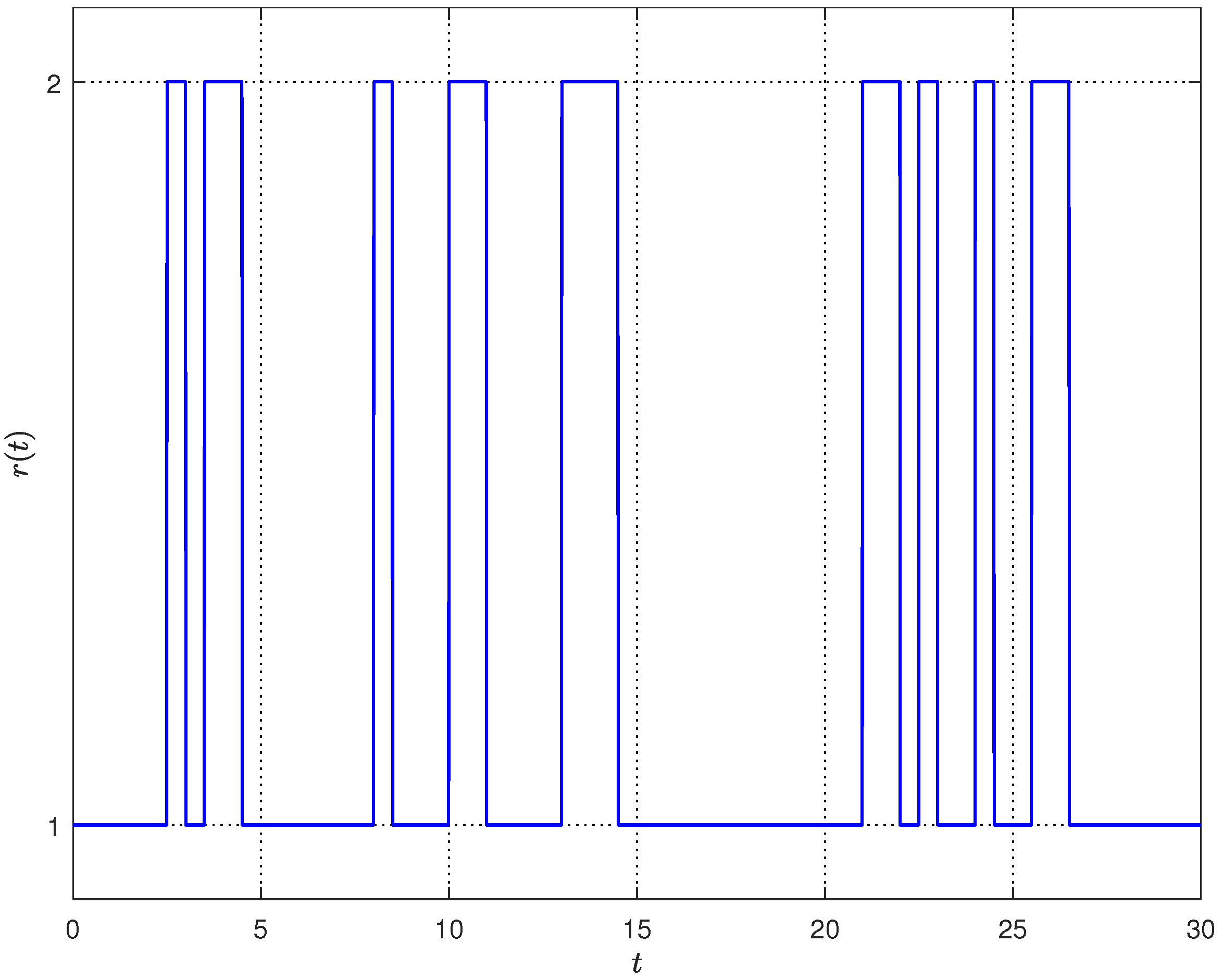
The two involved Markov processes r ( t ) and σ ( t ) with initial modes r 0 = 1 and σ 0 = 2 all follow exponential distribution. Meanwhile, their trajectories are shown in Figure 2 and Figure 3, respectively. Furthermore, relevant transition rate matrices can be set as
Λ ˇ = 0.4431 0.4431 0.8862 0.8862 , Λ = 0.2954 0.2954 0.4431 0.4431 .
In addition, take the uncertain parameter matrices as M 1 = M 2 = diag { 0.2 , 0.2 } , and
N 1 = 0.3 0.2 0.4 0.3 , N 2 = 0.2 0.4 0.3 0.3 ,
and F ( t , σ ( t ) ) refers to an unknown matrix satisfying the constraint F T ( t , σ ( t ) ) F ( t , σ ( t ) ) I .
By leveraging the aforementioned parameters, set r 1 = r 2 = ζ = 1 , and utilize MATLAB toolbox to solve the addressed constraints (8)–(10) from Theorem 1 and constraint (23) from Theorem 3; a number of viable solutions will be realized. Owing to space constraints, a portion of the results are provided below: γ = 0.9108 , φ = 1.2083 , Γ 1 = diag { 1.0698 , 1.2226 , 0.8252 , 0.8231 } , Γ 2 = diag { 1.1130 , 0.8672 , 0.8130 , 0.8130 } , N ^ 1 = [ 0.0778 0.0375 ] , N ^ 2 = [ 0.0755 0.0346 ] , and
P 11 = 0.5755 0.0655 0 0 0.0655 0.4338 0 0 0 0 0.3224 0.0609 0 0 0.0609 0.1929 , P 12 = 0.5905 0.0587 0 0 0.0587 0.4498 0 0 0 0 0.3224 0.0609 0 0 0.0609 0.1929 , P 21 = 0.5862 0.0524 0 0 0.0524 0.4266 0 0 0 0 0.3224 0.0609 0 0 0.0609 0.1929 , P 22 = 0.5956 0.0437 0 0 0.0437 0.4469 0 0 0 0 0.3224 0.0609 0 0 0.0609 0.1929 , Q 1 = 0.5705 0.0898 0.0115 0.0049 0.0898 0.4354 0.0035 0.0054 0.0115 0.0035 0.8137 0.0001 0.0049 0.0054 0.0001 0.8135 , Q 2 = 0.6584 0.1021 0.0135 0.0058 0.1021 0.4951 0.0040 0.0063 0.0135 0.0040 0.9254 0.0001 0.0058 0.0063 0.0001 0.9252 , Q 3 = 0.5705 0.0898 0.0115 0.0049 0.0898 0.4354 0.0035 0.0054 0.0115 0.0035 0.8137 0.0001 0.0049 0.0054 0.0001 0.8135 , R 1 = 0.8100 0.0019 0.0002 0.0001 0.0019 0.8072 0.0001 0.0001 0.0002 0.0001 0.8135 0.0000 0.0001 0.0001 0.0000 0.8135 , R 2 = 0.6649 0.0097 0.0008 0.0004 0.0097 0.6505 0.0004 0.0005 0.0008 0.0004 0.6828 0.0000 0.0004 0.0005 0.0000 0.6828 , X 3 = 0.0318 0.0003 0.0000 0.0000 0.0003 0.0313 0.0000 0.0000 0.0000 0.0000 0.0327 0.0000 0.0000 0.0000 0.0000 0.0327 , E ¯ 1 = 0.9602 0.0021 0.0002 0.0001 0.0021 0.9635 0.0001 0.0001 0.0002 0.0001 0.9562 0.0000 0.0001 0.0001 0.0000 0.9562 , X 2 = 0.3511 0.0040 0.0003 0.0002 0.0040 0.3572 0.0002 0.0002 0.0003 0.0002 0.3445 0.0000 0.0002 0.0002 0.0000 0.3445 , A ^ 1 = 1.7805 0.1450 0.1495 1.7705 , B ^ 1 = 0.0812 0.0998 0.0873 0.0415 , K ^ 1 = 2.9652 0.6074 0.3696 0.7390 , A ^ 2 = 1.7800 0.1547 0.1597 1.7703 , B ^ 2 = 0.0809 0.0989 0.0859 0.0400 , K ^ 2 = 2.9984 0.5615 0.2881 0.7611 .
Then, by resorting to the specific designed strategies (24), estimator gain matrices are able to be constructed as N 1 = [ 0.0778 0.0375 ] , N 2 = [ 0.0755 0.0346 ] , and
A 1 = 5.7182 2.3233 1.0311 9.9121 , B 1 = 0.1771 0.3723 0.3965 0.3325 , K 1 = 9.3973 2.7739 1.0521 4.7072 , A 2 = 5.7059 2.3551 0.9742 9.9214 , B 2 = 0.1775 0.3679 0.3890 0.3233 , K 2 = 9.5917 2.6454 1.5362 4.7811 .
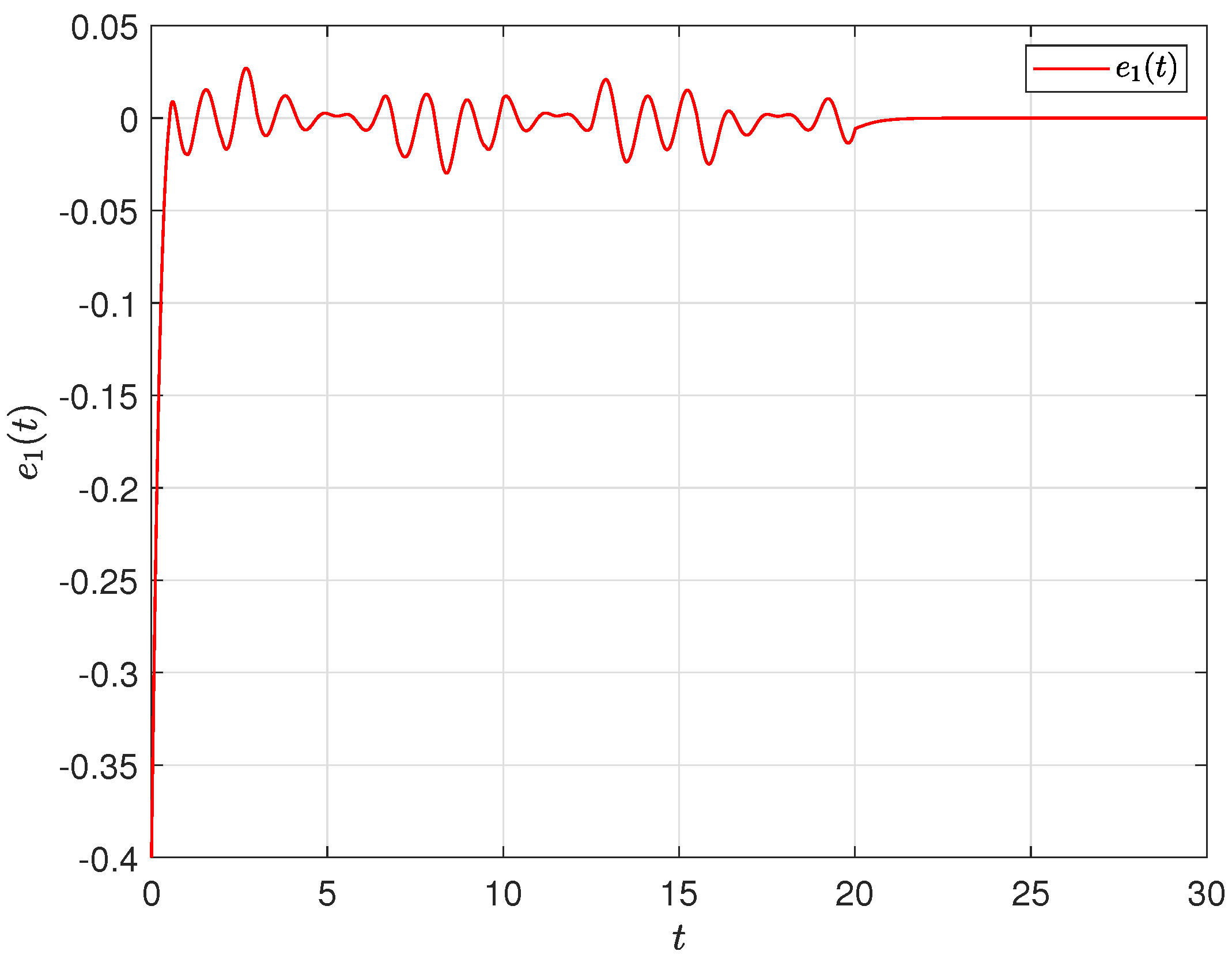
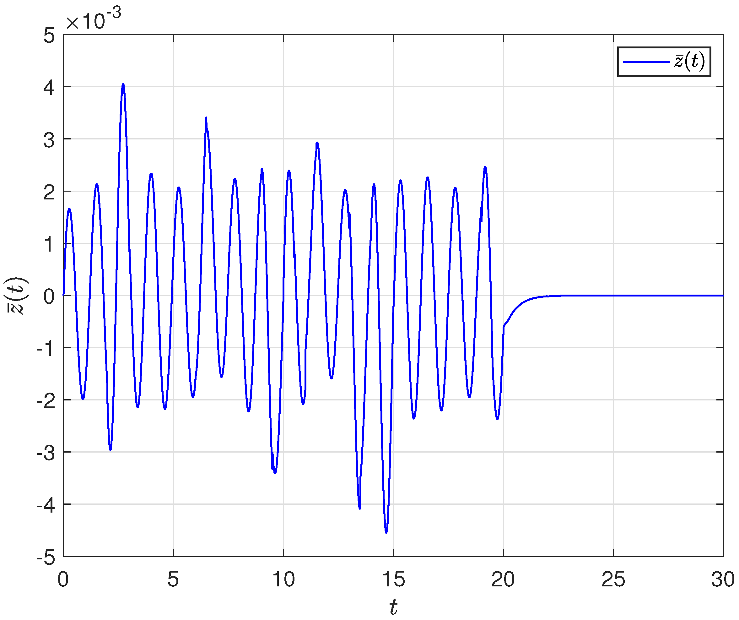
To enable a meaningful simulation, for system (1), initial constraint is specified as follows: set x ( s ) = [ 0.4 1.1 ] T , in which s [ 0.3 , 0 ] , x ˜ ( t ) = [ 0 0 ] T . Define e 1 ( t ) = x 1 ( t ) x ˜ 1 ( t ) and e 2 ( t ) = x 2 ( t ) x ˜ 2 ( t ) ; the trajectories of e 1 ( t ) and e 2 ( t ) are illustrated in Figure 4 as well as Figure 5, respectively, which can confirm that system (7) is capable of attaining global asymptotic mean-square stability. Alternatively, the external disturbances are defined as ω 1 ( t ) = 0.3 sin ( 6 t ) , ω 2 ( t ) = 0.4 sin ( 5 t ) , t [ 0 , 20 ) ; ω 1 ( t ) = ω 2 ( t ) = 0 , t [ 20 , ) . Taking the initial value as zero, Figure 6 illustrates the trajectory of the estimated output signal.

5. Conclusions

The purpose of this article is to address the non-fragile asynchronous H estimation issue for delayed Markovian jumping NNs subject to stochastic disturbance. To better model practical situations, external random disturbances with known statistical properties are introduced. Through the integration of stochastic analysis approaches, Lyapunov stability conclusion, and matrix restraint methodologies, several effective criteria can be established. These conditions ensure that the NNs achieve desired H stability in line with a prescribed external performance index. Moreover, necessary estimator gains can be explicitly constructed by working out the associated matrix inequalities. In the end, one reliable numerical simulation example has been added to authenticate applicability and soundness of introduced estimation scheme. Drawing on existing related accomplishments [6,18,32,44], our future work will tackle the asynchronous H estimation problem of Markovian jumping NNs through a significant event-triggered mechanism. This mechanism is capable of effectively reducing the communication burden on the network and conserving the limited communication resources.

Author Contributions

Methodology, J.T.; Writing—original draft, L.W.; Writing—review & editing, J.T., X.Y. and H.Z.; Visualization, Q.L.; Supervision, Q.L.; Funding acquisition, Q.L. and H.Z. All authors have read and agreed to the published version of the manuscript.

Funding

This research was partially supported by the National Natural Science Foundation of China (Grants 62406005 and 12426611), partially by the Natural Science Foundation of Anhui Province, China (Grant 2408085QA008), partially by the High-level Talent Research Foundation of Anhui Agricultural University (Grant rc382106), partially by the Yunnan Provincial Basic Research Program (Grants 202401AT070969 and 202201AU070046), and partially by the Open Foundation of Yunnan Key Laboratory of Intelligent Control and Application (Grant 2025ICA04).

Data Availability Statement

No new data were created or analyzed in this study.

Conflicts of Interest

The authors affirm that they are not cognizant of any opposing financial interests or personal links that may have appeared to impact the work outlined in this paper.

References

  1. Xia, Y.; Wang, J. A general projection neural network for solving monotone variational inequalities and related optimization problems. IEEE Trans. Neural Netw. 2004, 15, 318–328. [Google Scholar] [CrossRef] [PubMed]
  2. Xia, Y.; Feng, G. An improved neural network for convex quadratic optimization with application to real-time beamforming. Neurocomputing 2005, 64, 359–374. [Google Scholar] [CrossRef]
  3. Dou, H.; Shen, F.; Zhao, J.; Mu, X. Understanding neural network through neuron level visualization. Neural Netw. 2023, 168, 484–495. [Google Scholar] [CrossRef] [PubMed]
  4. Wang, J. Electronic realisation of recurrent neural network for solving simultaneous linear equations. Electron. Lett. 1992, 28, 493–495. [Google Scholar] [CrossRef]
  5. Li, X.; Song, S. Stabilization of delay systems: Delay-dependent impulsive control. IEEE Trans. Autom. Control 2018, 62, 406–411. [Google Scholar] [CrossRef]
  6. Wei, H.; Li, Q.; Zhu, S.; Fan, D.; Zheng, Y. Event triggered resilient asynchronous estimation of stochastic Markovian jumping CVNs with missing measurements: A co-design control strategy. Inf. Sci. 2025, 712, 122167. [Google Scholar] [CrossRef]
  7. Li, Q.; Wei, H.; Hua, D.; Wang, J.; Yang, J. Stabilization of semi-Markovian jumping uncertain complex-valued networks with time-varying delay: A sliding-mode control approach. Neural Process. Lett. 2024, 56, 111. [Google Scholar] [CrossRef]
  8. Abudireman, A.; Abdurahman, A. Fixed-time synchronization of spatiotemporal fuzzy neural network via aperiodic intermittent control with hyperbolic sine function. J. Appl. Math. Comput. 2025. [Google Scholar] [CrossRef]
  9. Abdurahman, A.; Abudusaimaiti, M.; Jiang, H. Fixed/predefined-time lag synchronization of complex-valued BAM neural networks with stochastic perturbations. Appl. Math. Comput. 2023, 444, 127811. [Google Scholar] [CrossRef]
  10. Jia, C.; Hu, J.; Yi, X.; Liu, H.; Huang, J.; Cao, Z. Recursive state estimation for a class of quantized coupled complex networks subject to missing measurements and amplify-and-forward relay. Inf. Sci. 2023, 630, 53–73. [Google Scholar] [CrossRef]
  11. Yu, X.; Sun, X.; Li, J. Scalable distributed data-driven state estimation algorithm via Gaussian processes with guaranteed stability. IEEE Trans. Aerosp. Electron. Syst. 2023, 59, 9191–9204. [Google Scholar] [CrossRef]
  12. Jia, C.; Hu, J.; Liu, H.; Du, J.; Feng, S. Recursive state estimation for a class of nonlinear uncertain coupled complex networks subject to random link failures and packet disorders. ISA Trans. 2022, 127, 88–98. [Google Scholar] [CrossRef]
  13. Hsieh, C.S. State estimation for descriptor systems via the unknown input filtering method. Automatica 2013, 49, 1281–1286. [Google Scholar] [CrossRef]
  14. Guo, Y.; Wang, Z.; Li, J.-Y.; Xu, Y. State estimation for Markovian jump neural networks under probabilistic bit flips: Allocating constrained bit rates. IEEE Trans. Neural Netw. Learn. Syst. 2025, 36, 8802–8813. [Google Scholar] [CrossRef] [PubMed]
  15. Zhang, F.; Zhang, Y. State estimation of neural networks with both time-varying delays and norm-bounded parameter uncertainties via a delay decomposition approach. Commun. Nonlinear Sci. Numer. Simul. 2013, 18, 3517–3529. [Google Scholar] [CrossRef]
  16. Xu, X.; Sun, J.; Wang, C.; Zou, B. A novel hybrid CNN-LSTM compensation model against DoS attacks in power system state estimation. Neural Process. Lett. 2022, 54, 1597–1621. [Google Scholar] [CrossRef]
  17. Sang, H.; Zhao, J. Energy-to-peak state estimation for switched neutral-type neural networks with sector condition via sampled-data information. IEEE Trans. Neural Networks Learn. Syst. 2021, 32, 1339–1350. [Google Scholar] [CrossRef]
  18. Hu, X.; Wei, X.; Zhang, H.; Gong, Q.; Sun, S. Event-triggered disturbance rejection tracking for surface ships under stochastic disturbances and actuator saturation. Int. J. Robust Nonlinear Control 2024, 34, 3207–3223. [Google Scholar] [CrossRef]
  19. Wu, Z.; Zhou, H.; Guo, B.; Deng, F. On the convergence of tracking differentiator with multiple stochastic disturbances. Sci. China Inf. Sci. 2024, 67, 122203. [Google Scholar] [CrossRef]
  20. Jia, C.; Wang, Z.; Hu, J.; Dong, H. Reputation-based distributed filtering over sensor networks subject to stochastic nonlinearity and network-induced quantization. IEEE Trans. Netw. Sci. Eng. 2025, 1–14. [Google Scholar] [CrossRef]
  21. Guo, B.; Xiao, Y. Synchronization of Markov switching inertial neural networks with mixed delays under aperiodically on-off adaptive control. Mathmatics 2023, 11, 2906. [Google Scholar] [CrossRef]
  22. Pan, L.; Hu, J.; Cao, J. Pinning synchronization of delayed neural networks via Markov switched control. Syst. Control Lett. 2024, 189, 105823. [Google Scholar] [CrossRef]
  23. Huang, M.; Dey, S. Dynamic quantizer design for hidden Markov state estimation via multiple sensors with fusion center feedback. IEEE Trans. Signal Process. 2006, 54, 2887–2896. [Google Scholar] [CrossRef]
  24. Peng, H.; Lu, R.; Shi, P. Synchronization control for coupled delayed neural networks with time-varying coupling via Markov pinning strategy. IEEE Syst. J. 2022, 16, 4071–4081. [Google Scholar] [CrossRef]
  25. Zhu, H.-N.; Zhang, C.-K.; Bin, N. Infinite horizon linear quadratic stochastic Nash differential games of Markov jump linear systems with its application. Int. J. Syst. Sci. 2014, 45, 1196–1201. [Google Scholar] [CrossRef]
  26. Xu, N.; Sun, L. Synchronization control of Markov jump neural networks with mixed time-varying delay and parameter uncertain based on sample point controller. Nonlinear Dyn. 2019, 98, 1877–1890. [Google Scholar] [CrossRef]
  27. Li, F.; Wang, Y.-N.; Shen, H. Dual event-triggered synchronization of two-time-scale jumping neural networks and its application in image encryption and decryption. IEEE Trans. Netw. Sci. Eng. 2025, 12, 943–954. [Google Scholar] [CrossRef]
  28. Wang, X.; Qin, Y.; Fang, T.; Shi, K.; Shen, H. Passive state estimation for Markov jumping inertial neural networks under fading channels. Int. J. Adapt. Control Signal Process. 2022, 36, 1603–1618. [Google Scholar] [CrossRef]
  29. Lakshmanan, S.; Park, J.H.; Ji, D.H.; Jung, H.Y.; Nagamani, G. State estimation of neural networks with time-varying delays and Markovian jumping parameter based on passivity theory. Nonlinear Dyn. 2012, 70, 1421–1434. [Google Scholar] [CrossRef]
  30. Yang, G.-H.; Wang, J.L. Robust nonfragile Kalman filtering for uncertain linear systems with estimator gain uncertainty. IEEE Trans. Autom. Control 2001, 46, 343–348. [Google Scholar] [CrossRef]
  31. Xiao, S.; Ge, X.; Han, Q.-L.; Zhang, Y. Distributed resilient estimator design for positive systems under topological attacks. IEEE Trans. Cybern. 2021, 51, 3676–3686. [Google Scholar] [CrossRef]
  32. Wang, F.; Liang, J.; Dobaie, A.M. Resilient filtering for time-varying stochastic coupling networks under the event-triggering scheduling. Int. J. Gen. Syst. 2018, 47, 491–505. [Google Scholar] [CrossRef]
  33. Zhao, C.; Zhong, S.; Zhang, X.; Zhong, Q.; Shi, K. Novel results on nonfragile sampled-data exponential synchronization for delayed complex dynamical networks. Int. J. Robust Nonlinear Control 2020, 30, 4022–4042. [Google Scholar] [CrossRef]
  34. Tan, G.; Wang, Z.; Xiao, S. Nonfragile extended dissipativity state estimator design for discrete-time neural networks with time-varying delay. Neurocomputing 2023, 539, 126206. [Google Scholar] [CrossRef]
  35. Han, X.-X.; Wu, K.-N.; Yuan, X. Asynchronous boundary stabilization of stochastic Markovian reaction-diffusion neural networks with mode-dependent delays. IEEE Trans. Neural Netw. Learn. Syst. 2025. [Google Scholar] [CrossRef] [PubMed]
  36. Han, X.-X.; Wu, K.-N.; Yuan, X. Observer-based asynchronous boundary stabilization for stochastic Markovian reaction Cdiffusion neural networks. IEEE Trans. Cybern. 2024, 54, 6667–6678. [Google Scholar] [CrossRef] [PubMed]
  37. Shi, X.; Wang, Z.; Han, L. Finite-time stochastic synchronization of time-delay neural networks with noise disturbance. Nonlinear Dyn. 2017, 88, 2747–2755. [Google Scholar] [CrossRef]
  38. Gu, K. An integral inequality in the stability problem of time-delay systems. In Proceedings of the 39th IEEE Conference on Decision and Control, Sydney, Australia, 12–15 December 2000; pp. 2805–2810. [Google Scholar]
  39. Zhang, X.-M.; Han, Q.-L. State estimation for static neural networks with time-varying delays based on an improved reciprocally convex inequality. IEEE Trans. Neural Networks Learn. Syst. 2018, 29, 1376–1381. [Google Scholar] [CrossRef]
  40. Li, Q.; Liang, J.; Qu, H. H estimation for stochastic semi-Markovian switching CVNNs with missing measurements and mode-dependent delays. Neural Netw. 2021, 141, 281–293. [Google Scholar] [CrossRef]
  41. Peng, D.; Li, X. Leader-following synchronization of complex dynamic networks via event-triggered impulsive control. Neurocomputing 2020, 412, 1–10. [Google Scholar] [CrossRef]
  42. Lin, A.; Cheng, J.; Park, J.H.; Yan, H.; Qi, W. Fault detection filtering of nonhomogeneous Markov switching memristive neural networks with output quantization. Inf. Sci. 2023, 632, 715–729. [Google Scholar] [CrossRef]
  43. Shen, H.; Huang, Z.; Cao, J.; Park, J.H. Exponential H filtering for continuous-time switched neural networks under persistent dwell-time switching regularity. IEEE Trans. Cybern. 2020, 50, 2440–2449. [Google Scholar] [CrossRef]
  44. Li, Q.; Liang, J.; Gong, W.; Wang, K.; Wang, J. Nonfragile state estimation for semi-Markovian switching CVNs with general uncertain transition rates: An event-triggered scheme. Math. Comput. Simul. 2024, 218, 204–222. [Google Scholar] [CrossRef]
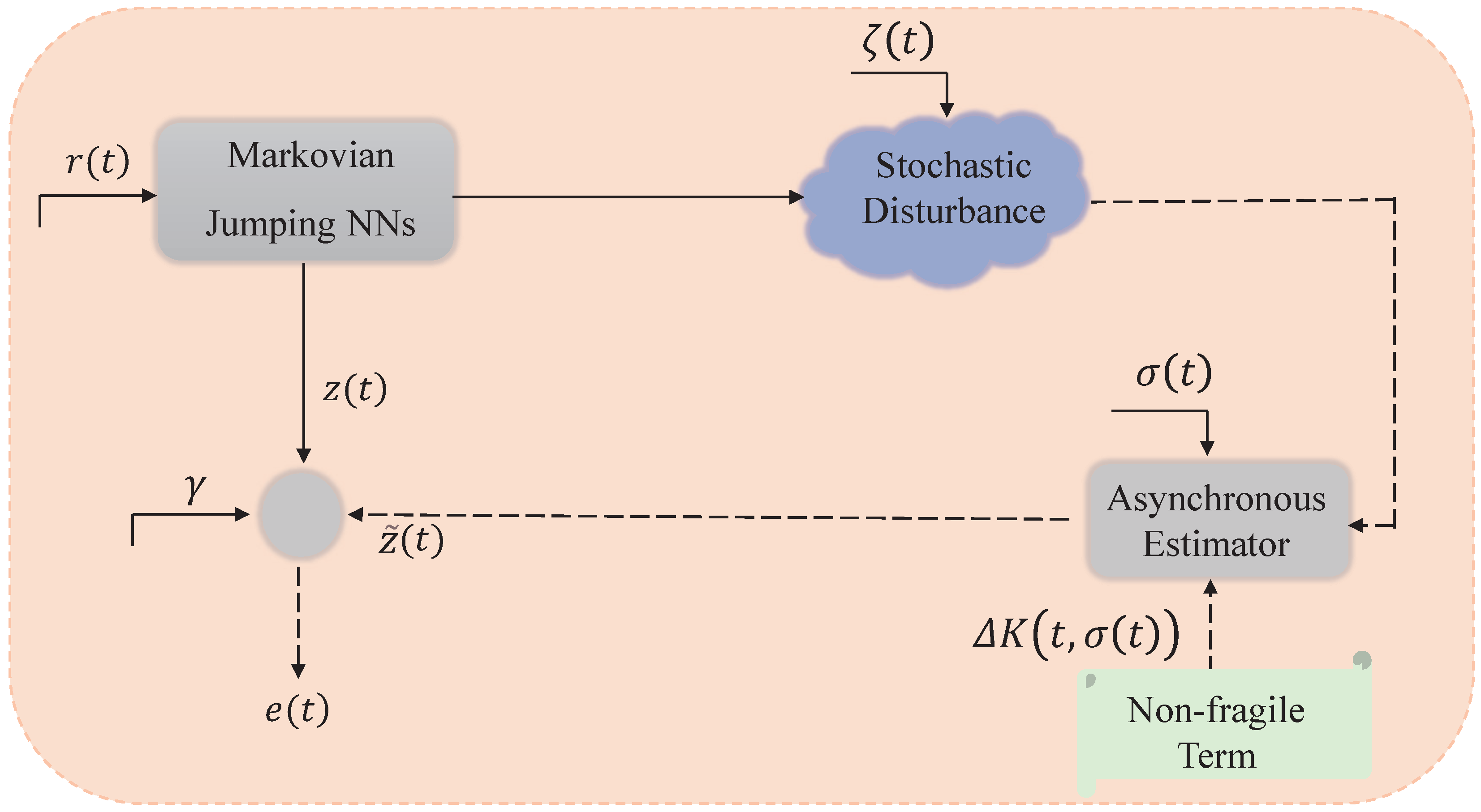
Figure 1. Framework of Markovian jumping NNs and asynchronous estimator.
Mathematics 13 02452 g001
Figure 2. Evolution of Markov process r ( t ) .
Mathematics 13 02452 g002
Figure 3. Evolution of Markov process σ ( t ) .
Mathematics 13 02452 g003
Figure 4. Evolution of error e 1 ( t ) .
Mathematics 13 02452 g004
Figure 5. Evolution of error e 2 ( t ) .
Mathematics 13 02452 g005
Figure 6. Illustration of system output z ¯ ( t ) .
Mathematics 13 02452 g006
Disclaimer/Publisher’s Note: The statements, opinions and data contained in all publications are solely those of the individual author(s) and contributor(s) and not of MDPI and/or the editor(s). MDPI and/or the editor(s) disclaim responsibility for any injury to people or property resulting from any ideas, methods, instructions or products referred to in the content.