Extra Connectivity and Extra Diagnosability of Enhanced Folded Hypercube-like Networks

Abstract

In the design of multiprocessor systems, evaluating the reliability of interconnection networks is a critical aspect that significantly impacts system performance and functionality. When quantifying the reliability of these networks, extra connectivity and extra diagnosability serve as fundamental metric parameters, offering valuable insights into the network’s resilience and fault-handling capabilities. In this paper, we investigate the 1-extra connectivity and 1-extra diagnosability of the n-dimensional enhanced folded hypercube-like network. Through analysis, we show that the 1-extra connectivity of this network is $2n+2$. Moreover, for $n>5$, we determine its 1-extra diagnosability under both the PMC model and the MM${}^{\ast }$ model to be $2n+3$. These results show that as the dimension n increases, both the 1-extra connectivity and 1-extra diagnosability of the network approach approximately twice the value of traditional diagnosability metrics. This provides quantitative insights into the reliability properties of the enhanced folded hypercube-like network, contributing to a better understanding of its performance in terms of connectivity and fault diagnosis.

1. Introduction

With the advancement of high-performance computing technology, the number of processors in interconnection networks is steadily growing. As the number of processors increases, it becomes highly likely that processors within interconnection networks will encounter failures. Reliability has been a crucial issue in interconnection networks. These networks’ reliability can be evaluated using two metrics: connectivity and diagnosability. In the study of network properties, we often use a graph G to represent the underlying network topology. A multiprocessor network typically consists of a number of processors and communication links. In graph G, we utilize nodes to represent processors and edges to represent the communication channels between them. G’s connectivity, denoted by $\kappa (G)$, is defined as the smallest number of nodes that, when removed, cause the remaining graph to become disconnected or reduce to a trivial graph. Based on this definition, it is theoretically possible for all the neighbors of a specific node to fail. However, the probability of all neighbors of a given node failing simultaneously is extremely small. As the network size grows, the traditional concept of connectivity becomes insufficient to accurately reflect the network’s fault-tolerance ability. To address this issue, many researchers have proposed various connectivity metrics under different constraints [1,2,3].

Another generalized concept of connectivity is the g-extra connectivity, which was proposed in [4]. It is also a new concept introduced to improve network fault tolerance. G’s g-extra connectivity ${\kappa }^g(G)$ refers to the minimum number of nodes that need to be removed to make G disconnected such that each remaining component contains at least $g+1$ nodes. Subsequently, Lv et al. [5] explored the g-extra connectivity of the $(n,k)$-star network; Yang et al. [6] proved the g-extra connectivity of hypercubes; and Zhu et al. [7] gave the g-extra connectivity of BC networks. Since BC networks include hypercubes, Möbius cubes, etc., the g-extra connectivity of these networks can be derived from the research results of Zhu et al. [7]. For the k-ary n-cube, when $k=2$, it is the n-dimensional hypercube network; when $k=3$, it contains triangles; when $k>4$, it does not contain triangles. Therefore, different values of g-extra connectivity can be obtained for different parameter ranges. Thus, Liu et al. [8] respectively studied the g-extra connectivity of k-ary n-cubes under different conditions $k\ge 4$ and $k=3$. The DQcube network is a composite network in which each node is replaced by an identical hypercube to form a new undirected disk network. Zhang and Meng [9] studied and obtained the g-extra connectivity of this network. Li et al. [10] obtained the g-extra connectivity of the data center network DCell; Lv et al. [11] studied the g-extra connectivity of the data center network BCDC; Zhou et al. [12] proved the g-extra connectivity of a class of recursive matching networks.

The process of identifying faulty processors by test results between processors is called system-level diagnosis. A system is termed t-diagnosable if the number of faulty processors does not exceed t, and all faulty units can be identified without replacement. The maximum number of faulty processors that a system can identify is denoted as its diagnosability [13]. Two well-known models have been proposed by various diagnosis strategies. The PMC model (P-M), first proposed by Preparata et al. in [14], is the earliest diagnostic framework. Under this model, two processors can mutually test each other if connected by an edge. Later, Sengupta and Dahbura [15] expanded the MM model and introduced the MM${}^{\ast }$ model (M-M). In the M-M, a processor adjacent to two other processors will perform tests on those two neighboring processors.

Generally, a system’s diagnosability corresponds to the neighborhood size of a specific node, which often limits the number of faulty processors it can identify. Moreover, the likelihood that all neighbors of a processor in the system fail simultaneously remains relatively low. Therefore, Lai et al. [16] devised a novel diagnosability measure, namely, conditional diagnosability. This measure is premised on the assumption that all the adjacent nodes of any given node cannot be faulty simultaneously. Thus, another classical generalization of diagnosability is the g-extra diagnosability (g-ED), first proposed in [17]. This concept imposes a constraint that each remaining component must contain at least $g+1$ nodes after removing faulty nodes, thereby further enhancing the system’s diagnostic capability. As a node-symmetric and edge-symmetric recursive network, the hypercube was proven by Zhang and Yang [17] to have g-ED under the P-M and M-M within specific ranges of g. Due to the complex structure of permutation graphs, studying their g-ED for general g is highly challenging. Consequently, Lin et al. [18] investigated the g-ED of permutation graphs for $g=1,2,3$ under both the P-M and M-M. Wang [19] further studied the g-ED of the Petersen graph under the M-M. For more research on other diagnosabilities, please refer to references [20,21].

Currently, many parallel computers with hypercubes as their underlying topological structure have been commercialized, such as Caltech’s Cosmicu [22] and Intel’s IPSC/2 [23]. With the continuous advancement of research, in recent years, data center networks based on hypercubes have also been emerging, such as the HSDC data center network [24] and BCDC data center network [25]. In the quest for higher-performance topological structures, folded hypercube-like networks, as a variant of hypercubes, have been proposed [26]. They include folded hypercubes, with a diameter about half that of hypercubes, and retain the hypercubes’ symmetry. Recently, enhanced folded hypercube-like networks (EFHNs), as an extension, have been put forward [27]. They keep the properties of the original folded hypercube-like networks, with recursive construction via hypercube-like structures. Their diameter is usually smaller, meaning shorter data transmission paths, lower communication latency, and higher parallel computing efficiency, meeting the high-performance needs of parallel computers in large-scale data-processing and complex tasks. Thus, studying their reliability is crucial. That is, exploring other properties of this network has significant research value. In this paper, we aim to explore the extra connectivity and the extra diagnosability of EFHNs under some conditions.

The structure of this paper is outlined as follows. Section 2 presents relevant notations, two diagnostic models, and the definition of EFHNs. In Section 3, we analyze the 1-extra connectivity of this network. Section 4 investigates its 1-ED under the P-M and M-M. Finally, we conclude the paper.

2. Preliminaries

This section presents the interpretations of certain symbols, details of two diagnostic models, and the definition of the EFHN. To simplify the discussion, the terms “networks” and “graphs”, along with “nodes” and “processors”, are used synonymously throughout the paper.

2.1. Notations

In this section, we present several basic terms and symbols that are applied in the entire paper. For convenience, we adopt the representation of a graph $G=(V(G),E(G))$ to illustrate the network topology. In this notation, $V(G)$ indicates the set of nodes in graph G, whereas $E(G)$ stands for the set of edges in G. Additionally, the number of elements in the set $V(G)$, symbolized by $|V(G)|$, is called the order of graph G, and the value of $|E(G)|$ is defined as the size of G. It is crucial to note that throughout this paper, our focus is solely on simple, finite, and undirected graphs, excluding other types of graphs from our discussions.

For any two nodes $v_1,v^1$$\in V(G)$, if there is an edge that links these two nodes, we can claim that $k_1$ and $k^1$ are adjacent, or they are neighbors of each other. This relationship can be symbolized as $(v_1,v^1)$$\in E(G)$. For an arbitrary node $v_1$ in graph G, we denote its neighborhood as $N_G(v_1)$. This set consists of all nodes that are adjacent to $v_1$. That is, $N_G(v_1)=\{v^1\in V(G)|(v_1,v^1)\in E(G)\}$. Similarly, when considering any subset of nodes S in graph G, its neighborhood, denoted as $N_G(S)$, represents the set of nodes that are adjacent to at least one node within the subset S. More precisely, $N_G(S)=\{v^1\in V(G)|\exists v_1\in S$, $(v_1,v^1)\in E(G)\}-S={\bigcup }_{v_1\in S}{N}_G(v_1)-S$. For $v_1\in V(G),S\subseteq V(G)$, we define $N_G\left[v_1\right]=N_G(v_1)\cup \left\{v_1\right\}$ and $N_G\left[S\right]=N_G(S)\cup S$. The degree of node $v_1$ in graph G, denoted by $d_G(v_1)$, refers to the number of edges that are incident to $v_1$. Given that G is a simple graph, we can conclude that $d_G(v_1)=\left|N_G(v_1)\right|$. The minimum degree of G is determined by $\delta (G)=min\left\{d_G(v_1)\right|v_1\in V(G)\}$.

Moreover, for any two nodes $v_1$ and $v^1$ in graph G, the notation $|N_G(v_1)\cap N_G(v^1)|$ is used to represent the number of common neighbors between them. For the sake of simplicity in our discussions, we define $\langle \mathfrak{s}\rangle =\{0,1,\dots ,\mathfrak{s}\}$ and $\left[\mathfrak{s}\right]=\{1,2,\dots ,\mathfrak{s}\}$.

2.2. Two Diagnostic Models

In what follows, we present two well-known diagnostic models. Specifically, these are the P-M and the M-M.

Definition 1

([17]). A node subset N of graph G is a g-extra node subset if and only if every component of $G-N$ has more than g nodes.

Definition 2

([17]). $G=(V,E)$ is h-extra t-diagnosable if and only if for each pair of distinct faulty g-extra node subsets $N_1,N_2\subseteq V(G)$ such that if $|N_1|,|N_2|\le t$, $N_1$ and $N_2$ are distinguishable. The g-ED of G, denoted as $t_g(G)$, is the maximum value of t such that G is g-extra t-diagnosable.

2.2.1. PMC Model

Under the P-M, the testing process is carried out between two neighboring processors. We use the ordered pair $\overline{(v_1,v^1)}$ to represent that the node $v_1$ conducts a test on the node $v^1$ and $\sigma (v_1,v^1)$ to denote the test result. When the node $v_1$ operates without faults, the test result is reliable. In terms of representing the test results, if the node $v^1$ is fault-free under this circumstance, we assign $\sigma (v_1,v^1)=0$; conversely, if the node $v^1$ has faults, we assign $\sigma (v_1,v^1)=1$.

Theorem 1

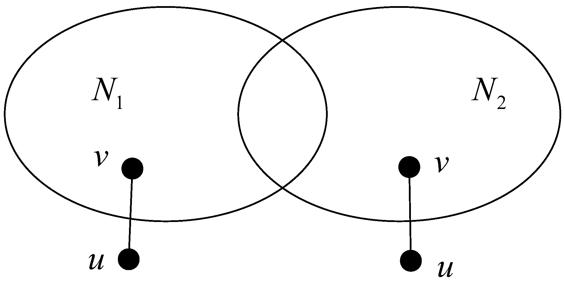
([28]). For $N_1,N_2\subseteq V(G)$, $(N_1,N_2)$ is a distinguishable pair of G under P-M if and only if there is a node $u\in V-(N_1\cup N_2)$ and a node $v\in N_1\Delta N_2$ such that $(u,v)\in E$ (see Figure 1).

2.2.2. MM${}^{\ast }$ Model

The MM model involves a node w with two neighbors u and v; w sends the same diagnostic information to u and v, and compares their responses. For convenience, we use $\sigma (w;u,v)$ to denote the test result. Non-faulty nodes return identical results, while faulty nodes may return different ones. If u and v return the same result, they are considered non-faulty (recorded as $\sigma (w;u,v)=0$); if they are different, at least one is faulty (recorded as $\sigma (w;u,v)=1$). Additionally, the M-M is a variant of MM that requires every 2-path’s middle node w to perform diagnosis without exception.

Theorem 2

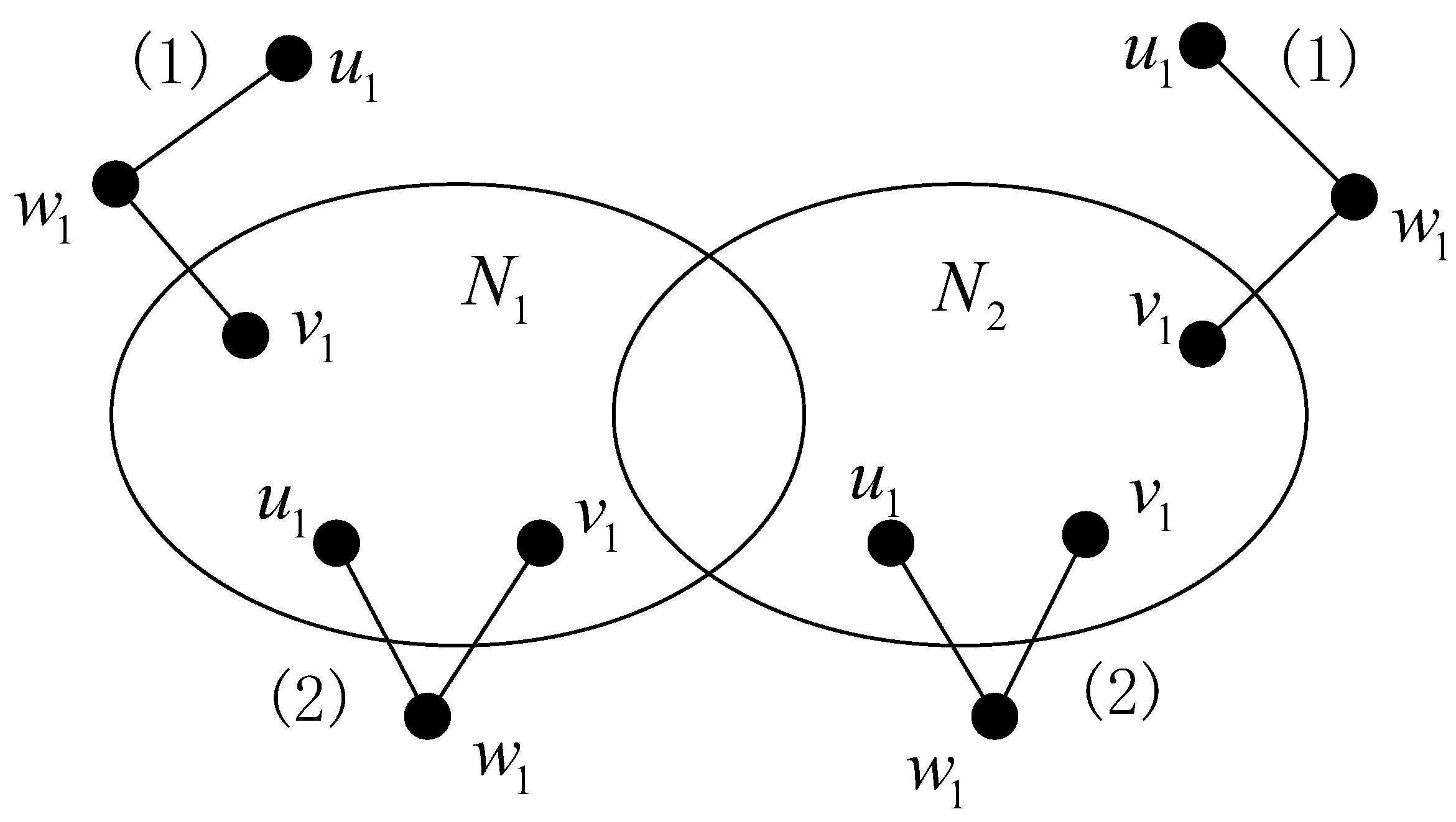
([15]). For $N_1,N_2\subseteq V(G)$, $(N_1,N_2)$ is a distinguishable pair under M-M if and only if one of the following conditions is satisfied (see Figure 2):

(1) 

There are two nodes $u_1,w_1\in V(G)-(N_1\cup N_2)$ and there is a node $v_1\in N_1\Delta N_2$ such that $(u_1,w_1)\in E(G)$ and $(v_1,w_1)\in E(G)$;

(2) 

There are two nodes $u_1,v_1\in N_j-N_{1-j}$ and there is a node $w_1\in V(G)-(N_j\cup N_{1-j})$ such that $(u_1,w_1)\in E(G)$ and $(v_1,w_1)\in E(G)$ for $j\in \{0,1\}$.

Figure 2. Illustration of distinguishability under the M-M.

Figure 2. Illustration of distinguishability under the M-M.

In summary, how these models work is mainly based on testing the connections between nodes. Under the P-M, if two nodes are connected by an edge, they can test each other. Under the M-M, if a node has two different neighboring nodes, it can test its two neighboring nodes. The specific testing rules for these two modes are described above, respectively. In addition, for ease of understanding, the following is a brief introduction to why the conditions listed in Theorems 1 and 2 are sufficient to guarantee distinguishability.

P-M: (Sufficiency) If $v_1\in N_1-N_2$ then $\sigma (u_1,v_1)=0$ when $N_2$ is the fault set, whereas $\sigma (u_1,v_1)=1$ when $N_1$ is the fault set. Similarly, if $v_1\in N_2-N_1$, then $\sigma (u_1,v_1)=0$ when $N_1$ is the fault set, whereas $\sigma (u_1,v_1)=1$ when $N_2$ is the fault set. In either case, $\sigma (N_1)\cap (N_2)=0$.

M-M: (Sufficiency) Suppose that condition (1) is satisfied. If $v_1\in N_1-N_2$, then $\sigma (w_1;u_1,v_1)=0$ when $N_2$ is the fault set, whereas $\sigma (w_1;u_1,v_1)=1$ when $N_1$ is the fault set. Hence $\sigma (N_1)\cap (N_2)=0$. A similar argument can be used when $v_1\in N_2-N_1$. Suppose that condition (2) is satisfied. If $v_1\in N_1-N_2$ then $\sigma (w_1;u_1,v_1)=0$ when $N_2$ is the fault set, whereas $\sigma (w_1;u_1,v_1)=1$ when $N_1$ is the fault set. Similarly, if $v_1\in N_2-N_1$, then $\sigma (w_1;u_1,v_1)=0$ when $N_1$ is the fault set, whereas $\sigma (w_1;u_1,v_1)=1$ when $N_2$ is the fault set. In either case, $\sigma (N_1)\cap (N_2)=0$.

2.3. The Folded Hypercube-like Network

The definition of the n-dimensional folded hypercube-like network $F{H}_n$ is presented.

Theorem 3

([26]). $F{H}_n$ is defined recursively:

(1) Let $X_1$ be an edge on two nodes labeled by 0 and 1. Let $L_1=\left\{X_1\right\}$.

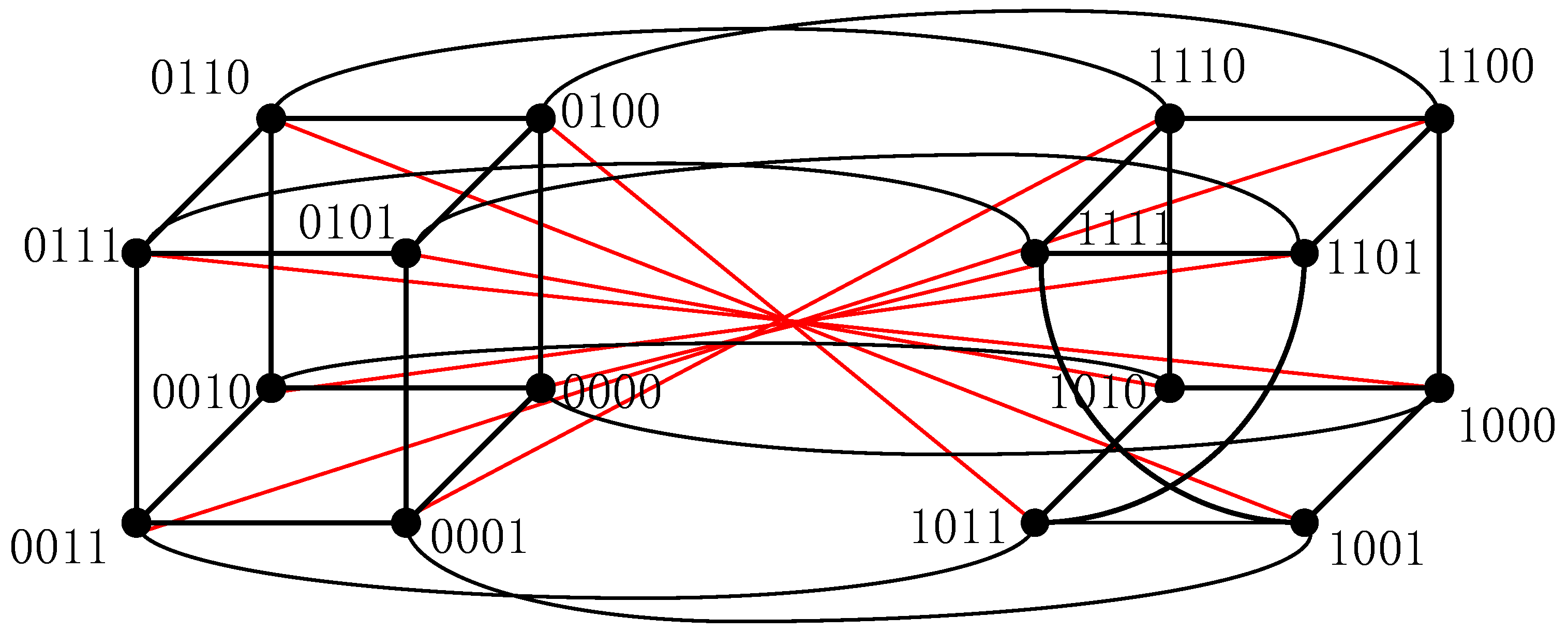
(2) Construct two instances of $X_1$: Create $X_1^0$ by prefixing labels with 0, resulting in an edge connecting nodes labeled 00 and 01. Similarly, form $X_1^1$ by prefixing labels with 1, yielding edge connecting nodes labeled 10 and 11. Add a perfect matching between $X_1^0$ and $X_1^1$ such that no edges from $\overline{M}$ are included. Denote the resulting graph as $X_2$, which is isomorphic to a 4-cycle (see Figure 1). Define $L_2=\left\{X_2\right\}$.

(3) To construct $X_3$, duplicate $X_2$ into $X_2^0$ and $X_2^1$ by prepending 0 and 1 to all node labels, respectively. Connect these copies with a perfect matching that excludes edges from $\overline{M}$. The resulting graph $X_3$ is isomorphic to either the 3-dimensional hypercube $Q_3$ or the 3-dimensional crossed cube $C{Q}_3$. Define $L_3=\{Q_3,C{Q}_3\}$.

(4) Construct two graphs by selecting one graph from $L_3$ each, denoted as $X_3^0$ and $X_3^1$, where labels are prefixed with 0 and 1 respectively. Note that $X_3^0$ and $X_3^1$ are not necessarily isomorphic. Add a perfect matching between $X_3^0$ and $X_3^1$ such that no edges from M are included. Denote the resulting graph as $X_4$. Define $L_4$ as the set of all possible graphs $X_4$ constructed via this method.

(5) To generate $L_t$, replicate the procedure in Step (4) using two graphs from $L_{t-1}$, terminating at $t=n-1$. For $L_{n-1}$, select two graphs to form $X_{n-1}^0$ and $X_{n-1}^1$. Connect these via a perfect matching excluding edges from $\overline{M}$, then append the matching $\overline{M}$. The resultant n-dimensional structure is denoted as $F{H}_n=X_{n-1}^0⨀X_{n-1}^1$, $F{H}_n$ being composed of two $(n-1)$-dimensional hypercube-like subgraphs (see Figure 3).

To facilitate understanding of the definition of the $F{H}_n$ network, we present the following algorithm for constructing the network. A similar algorithm can be provided for constructing an $EF{H}_n$ network. Therefore, we will not repeat the description here (see Algorithm 1).

Algorithm 1 $ConstructFH$ (n)

Input: Integer $n\ge 1$.

Output:  $F{H}_n$ network structure.

1: function $ConstructFH$ (n)

2:       if $n=1$ then;

3:             $X_1\leftarrow$ Edge connecting nodes labeled 0 and 1;

4:             $L_1\leftarrow \left\{X_1\right\}$;

5:             return $L_1$;

6:         end if

7:         $F{H}_{n-1}$ ← $ConstructFH(n-1)$;

8:         $X_{n-1}^0$ ← Graph obtained by prefixing all node labels in $F{H}_{n-1}$ with 0;

9:         $X_{n-1}^1$ ← Graph obtained by prefixing all node labels in $F{H}_{n-1}$ with 1;

10:         Add a perfect matching M connecting $X_{n-1}^0$ and $X_{n-1}^1$, where M does not

include edges from set $\overline{M}$, and then append the matching $\overline{M}$;

11:         $F{H}_n$ ← Graph formed by connecting $X_{n-1}^0$ and $X_{n-1}^1$ with perfect matchings M

and $\overline{M}$;

12:         return $F{H}_n$;

13: end function

Proposition 1

([26]). For $n\ge 2$,

(1) $|V(F{H}_n)|=2^n$ and $|E(F{H}_n)|=(n+1)2^{n-1}$;

(2) $F{H}_n$ is $(n+1)$-regular;

(3) $g(FHn)\ge 3$;

(4) $|N_{F{H}_n}(x^1)\cap N_{F{H}_n}(x^2)|\le 2$ for any $x^1,x^2\in V(F{H}_n)$;

(5) Each node of $X_{n-1}^0$ has only two neighbors in $X_{n-1}^1$, and similarly, each node of $X_{n-1}^1$ also has only two neighbors in $X_{n-1}^0$.

Definition 4

([27]). The n-dimensional EFHN $EF{H}_n$ can be defined recursively:

(1) Create two instances of $F{H}_n$: Form $F{H}_{n-1}^0$ by prefixing labels with 0, and similarly derive $F{H}_{n-1}^1$ by prefixing labels with 1.

(2) Connect $F{H}_{n-1}^0$ and $F{H}_{n-1}^1$ with a perfect matching $\overline{M}$, then add another perfect matching M between the two. The resulting graph is denoted as $EF{H}_n=F{H}_{n-1}^0⨁F{H}_{n-1}^1$ (see Figure 4).

Proposition 2

([27]). For $n\ge 2$,

(1) $|V(EF{H}_n)|=2^n$ and $|E(EF{H}_n)|=(n+2)2^{n-1}$;

(2) $EF{H}_n$ is $(n+2)$-regular;

(3) $g(EF{H}_n)\ge 3$;

(4) $|N_{EF{H}_n}(x^1)\cap N_{EF{H}_n}(x^2)|\le 2$ for any $x^1,x^2\in V(EF{H}_n)(n\ge 5)$.

3. The 1-Extra Connectivity of EFHNs

Next, we will show the 1-extra connectivity of EFHNs. Before that, some well-known lemmas are first presented.

Lemma 1

([29]). Let $X_n$ be an n-dimensional hypercube-like network. $\kappa (X_n)=n$ for $n\ge 2$.

Lemma 2

([30]). For $n\ge 3$.

(1) ${\kappa }^1(X_n)=2n-2$;

(2) ${\kappa }^3(X_n)=2n-2$.

Lemma 3

([26]). $\kappa (F{H}_n)=\lambda (F{H}_n)=n+1$ for $n\ge 2$.

Lemma 4

([27]). $\kappa (EF{H}_n)=\lambda (EF{H}_n)=n+2$ for $n\ge 2$.

Lemma 5

([7]). Let $m\ge 4$, for any $X_m$, $R\subseteq V(X_m)$ with $\left|R\right|\le my-{\displaystyle \frac{1}{2}}(y-1)(y+2)-1$, then $X_m-R$ has a large component $\mathbb{M}$ containing at least $\left|V(\mathbb{M})\right|\ge 2^m-\left|R\right|-(y-1)$, where $1\le y\le m-3$.

Lemma 6.

For $g(EF{H}_n)\ge 4$, $|N_{EF{H}_n}(H)|\ge 2n+2$ for any $H\subseteq V(EF{H}_n)$ with $\left|H\right|=2$.

Proof. 

Without loss of generality, let $H=\{y_1,y_2\}$. According to whether there is an edge connecting $y_1$ and $y_2$, the following cases are presented.

Case 1. $(y_1,y_2)\notin E(F{H}_n)$.

By Proposition 2, since $|N_{EF{H}_n}(y_1)\cap N_{EF{H}_n}(y_2)|\le 2$ and $(y_1,y_2)\notin E(EF{H}_n)$,

$$\begin{array}{ccc}\hfill |N_{EF{H}_n}(H)|& =& |N_{EF{H}_n}(y_1)|+|N_{EF{H}_n}(y_2)|-|N_{EF{H}_n}(y_1)\cap N_{EF{H}_n}(y_2)|\hfill \\ \hfill & \ge & n+2+n+2-2=2n+2.\hfill \end{array}$$

Case 2. $(y_1,y_2)\in E(EF{H}_n)$.

By Proposition 2, since $(y_1,y_2)\in E(EF{H}_n)$ and $g(EF{H}_n)\ge 4$, $|N_{EF{H}_n}(y_1)\cap N_{EF{H}_n}(y_2)|=0.$ Thus,

$$\begin{array}{ccc}\hfill |N_{EF{H}_n}(H)|& =& |N_{EF{H}_n}(y_1)|+|N_{EF{H}_n}(y_2)|-|N_{EF{H}_n}(y_1)\cap N_{EF{H}_n}(y_2)|-|\{y_1,y_2\}|\hfill \\ \hfill & \ge & n+2+n+2-0-2=2n+2.\hfill \end{array}$$

□

Lemma 7.

For $g(F{H}_n)\ge 4$, $n\ge 5$, and $H\subseteq V(F{H}_n)$ with $\left|H\right|\le 2n-1$, $F{H}_n-H$ satisfies one of the following conditions:

(1) $F{H}_n-H$ is connected.

(2) $F{H}_n-H$ has exactly two components, one of which is an isolated node.

Proof. 

Since $V(F{H}_n)=V(X_{n-1}^0)\cup V(X_{n-1}^1)$, let $H_0=V(X_{n-1}^0)\cap H$ and $H_1=V(X_{n-1}^1)\cap H$. Thus, $H=H_0\cup H_1$.

Case 1. Both $X_{n-1}^0-H_0$ and $X_{n-1}^1-H_1$ are connected.

Since $X_{n-1}^i-H_i$ is connected and $|V(X_{n-1}^i)|=2^{n-1}>2n-1$ for each $i\in \{0,1\}$ and $n\ge 5$, $X_{n-1}^0-H_0$ is connected to $X_{n-1}^1-H_1$, namely, $F{H}_n-H$ is connected, a contradiction.

Case 2. Both $X_{n-1}^0-H_0$ and $X_{n-1}^1-H_1$ are disconnected.

By Lemma 1, $\kappa (X_n)=n$. Since both $X_{n-1}^0-H_0$ and $X_{n-1}^1-H_1$ are disconnected, $n-1\le |H_0|\ge 2n-1$ and $n-1\le |H_1|\ge 2n-1$. Additionally, $|H_0|\le 2n-5$ and $|H_1|\le 2n-5$; otherwise, it will be in contradiction with $n-1\le |H_0|$ and $n-1\le |H_1|$ for $n\ge 5$. In word, $n-1\le |H_0|\ge 2n-5$ and $n-1\le |H_1|\ge 2n-5$. By Lemma 5, $X_{n-1}^0-H_0$ (respectively $X_{n-1}^1-H_1$) has only two components, one of which is an isolated node, say $h_0$ (respectively $h_1$) in $X_{n-1}^0-H_0$ (respectively $X_{n-1}^1-H_1$). Since $V(X_{n-1}^0)-|H_0|-|\left\{h_0\right\}|>2n-1$, $X_{n-1}^0-H_0$ is connected to $X_{n-1}^1-H_1$. We say $h_0$ or $h_1$ is connected to $F{H}_n-H-\{h_0,h_1\}$. By contrast, $h_0$ and $h_1$ are disconnected to $F{H}_n-H-\{h_0,h_1\}$. Then, $N_{F{H}_n}(\{h_0,h_1\})\subseteq H$. That is, $\left|H\right|\ge |N_{F{H}_n}(\{h_0,h_1\})|\ge 2n$, a contradiction. Therefore, there is at most one isolated node in $F{H}_n-H$.

Case 3. $X_{n-1}^i-H_i$ is connected and $X_{n-1}^{1-i}-H_{1-i}$ is disconnected for $i\in \{0,1\}$.

Without loss of generality, let $X_{n-1}^0-H_0$ be connected and $X_{n-1}^1-H_1$ be disconnected. Then, $2n-1\ge |H_1|\ge n-1$ and $|H_0|\le n$ by Lemma 1.

Subcase 3.1. $n-1\le |H_1|\le 2n-5$.

By Lemma 5, $X_{n-1}^1-H_1$ has a large connected component containing at least $2^{n-1}-\left|H_1\right|-1$ nodes for $|H_1|\le 2n-5$. Therefore, when $X_{n-1}^1-H_1$ is disconnected, $X_{n-1}^1-H_1$ has a large connected component containing $2^{n-1}-\left|H_1\right|$ nodes and an isolated node, denoted by x. On the other hand, because $X_{n-1}^0-H_0$ is connected and $|V(X_{n-1}^0)|-|H_0|-|\left\{x\right\}|-n-1=2^{n-1}-n-1>2n-1=\left|H\right|$, $X_{n-1}^0-H_0$ is disconnected to $X_{n-1}^1-H_1-\left\{x\right\}$. If the isolated node x is connected to $X_{n-1}^0-H_0$, then $F{H}_n-H$ is connected; otherwise, $F{H}_n-H$ has only two components, one of which is an isolated node x.

Subcase 3.2. $2n-4\le |H_1|\le 2n-1$.

Since $2n-4\le |H_1|\le 2n-1$, $|H_0|\le 2n-1-(2n-4)=3$. According to Definition 3, there exists at most one node in $X_{n-1}^1$ whose neighbors in $X_{n-1}^0$ are all located in $H_1$. If this node exists in $X_{n-1}^1$, then we denote it as v. Therefore, each node in $V(X_{n-1}^0)-\left\{v\right\}$ is connected to $X_{n-1}^0-H_0$. In a word, $F{H}_n-H$ is connected or $F{H}_n-H$ has only two components, one of which is an isolated node v. □

Lemma 8.

For $g(EF{H}_n)\ge 4$, $n\ge 5$, and $H\subseteq V(EF{H}_n)$ with $\left|H\right|\le 2n+1$, $EF{H}_n-H$ satisfies one of the following conditions:

(1) $EF{H}_n-H$ is connected.

(2) $EF{H}_n-H$ has exactly two components, one of which is an isolated node.

Proof. 

Since $V(EF{H}_n)=V(F{H}_{n-1}^0)\cup V(F{H}_{n-1}^1)$, we set $H_0=V(F{H}_{n-1}^0)\cap H$ and $H_1=V(F{H}_{n-1}^1)\cap H$. Thus, $H=H_0\cup H_1$. We discuss the following cases based on whether $F{H}_{n-1}^i-H_i$ is connected for $i\in \{0,1\}$.

Case 1. Both $F{H}_{n-1}^0-H_0$ and $F{H}_{n-1}^1-H_1$ are connected.

Let $T_0$ be the connected component in $F{H}_{n-1}^0-H_0$, and $T_1$ be the connected component in $F{H}_{n-1}^1-H_1$. Since $F{H}_{n-1}^i-H_i$ is connected and $|V(F{H}_{n-1}^i)|=2^{n-1}>2n+1$ for each $i\in \{0,1\}$ and $n\ge 5$, $T_0$ is connected to $T_1$, that is, $EF{H}_n-H$ is connected.

Case 2. Both $F{H}_{n-1}^0-H_0$ and $F{H}_{n-1}^1-H_1$ are disconnected.

Since both $F{H}_{n-1}^0-H_0$ and $F{H}_{n-1}^1-H_1$ are disconnected, $n\le |H_0|\le 2n+1$ and $n\le |H_1|\le 2n+1$ by Lemma 3.

Subcase 2.1. $|H_0|=|H_1|=n$.

Since $|H_0|=|H_1|=n$, $F{H}_{n-1}^0-H_0$ (respectively, $F{H}_{n-1}^1-H_1$) has only two components, one of which is an isolated node, say $h_0$ (respectively, $h_1$) in $F{H}_{n-1}^0-H_0$ (respectively, $F{H}_{n-1}^1-H_1$) by Lemma 7. Let $T_i$ be the component in $F{H}_{n-1}^i-H_i-\left\{h_i\right\}$ for $i\in \{0,1\}$. Therefore, $|V(T_i)|=|V(F{H}_{n-1}^i)|-|H_i|-|\left\{h_i\right\}|=2^{n-1}-n-1>2n-1\ge \left|H\right|$ for each $i\in \{0,1\}$. Thus, $T_0$ is connected to $T_1$.

(1) If $h_i$ is connected to $T_{1-i}$, then $EF{H}_n-H$ is connected for each $i\in \{0,1\}$.

(2) If $h_i$ is connected to $T_{1-i}$ and $h_{1-i}$ is disconnected to $T_i$ and $h_i$, then $EF{H}_n-H$ has exactly two components, one of which is an isolated node $h_{1-i}$ for each $i\in \{0,1\}$ (see Figure 5a).

(3) If $h_i$ is connected to $T_{1-i}$, $h_{1-i}$ is connected to $T_i$, and $h_{1-i}$ is disconnected to $h_i$, then $EF{H}_n-H$ is connected for each $i\in \{0,1\}$ (see Figure 5b).

(4) If $h_i$ is connected to $T_{1-i}$, $h_{1-i}$ is connected to $h_i$, and $h_{1-i}$ is disconnected to $T_i$, then $EF{H}_n-H$ is connected for each $i\in \{0,1\}$ (see Figure 5c).

(5) If $h_i$ is disconnected to $T_{1-i}$ for each $i\in \{0,1\}$, then $N_{EF{H}_n}(\{h_0,h_1\})\subseteq H$, that is, $|N_{EF{H}_n}(\{h_0,h_1\}|\le |H|\le 2n+1$. However, $|N_{EF{H}_n}(\{h_0,h_1\}|\ge 2n+2$ by Lemma 6. Hence, $h_0$ is connected to $T_1$, or $h_1$ is connected to $T_0$ (see Figure 5d).

Subcase 2.2. $|H_0|=n$ and $|H_1|=n+1$.

Since $|H_0|=n\le 2n-3$ and $|H_1|=n+1\le 2n-3$, $F{H}_{n-1}^0-H_0$ and $F{H}_{n-1}^1-H_1$ have only two components, one of which is an isolated node, say $h_0$ and $h_1$ in $F{H}_{n-1}^0-H_0$ and $F{H}_{n-1}^1-H_1$ by Lemma 7, respectively. Therefore, similar to the discussion in Subcase 2.1, it can be concluded that this lemma holds.

Subcase 2.3. $|H_0|=n+1$ and $|H_1|=n$.

Analogous to Subcase 2.2, we can deduce that this lemma is valid.

Case 3. $F{H}_{n-1}^i-H_i$ is connected, and $F{H}_{n-1}^{1-i}-H_{1-i}$ is disconnected for $i\in \{0,1\}$.

Without loss of generality, let $F{H}_{n-1}^0-H_0$ be connected and $F{H}_{n-1}^1-H_1$ be disconnected. Since $F{H}_{n-1}^1-H_1$ is disconnected, $n\le |H_1|\le 2n+1$ and $|H_0|\le n+1$.

Subcase 3.1. $n\le |H_1|\le 2n-3$.

By Lemma 7, since $F{H}_{n-1}^1-H_1$ is disconnected, $F{H}_{n-1}-H_1$ has exactly two components, one of which is an isolated node, say $h_1$ in $F{H}_{n-1}^1-H_1$. On the other hand, because $|V(F{H}_{n-1}^0)|-|H_0|\ge 2^{n-1}-(n+1)>2n-1\ge \left|H\right|$, $F{H}_{n-1}^0-H_0$ is connected to $F{H}_{n-1}^1-H_1-\left\{h_1\right\}$. In this case, if $h_1$ is connected to $F{H}_{n-1}^0-H_0$, then $EF{H}_n-H$ is connected; otherwise, $EF{H}_n-H$ has exactly two components, one of which is an isolated node $h_1$.

Subcase 3.2. $2n-2\le |H_1|\le 2n+1$.

Since $2n-2\le |H_1|\le 2n+1$, $|H_0|\le |H|-|H_1|\le 2n-1-(2n-4)=3$. Therefore, $F{H}_{n-1}^0-H_0$ is connected. According to Definition 4, there exists at most one node in $F{H}_{n-1}^1$ whose neighbors in $F{H}_{n-1}^0$ are all located in $H_1$. If this node exists in $F{H}_{n-1}^1$, then we denote it as y. Therefore, each node in $V(F{H}_{n-1}^0)-\left\{y\right\}$ is connected to $F{H}_{n-1}^0-H_0$. In a word, $EF{H}_n-H$ is connected or $EF{H}_n-H$ has only two components, one of which is an isolated node y. □

Lemma 8 obtains the size of each component in the remaining graph of EFH${}_n$ after deleting up to $2n+1$ nodes. Building on the results of Lemma 8, we derive the following theorem.

Theorem 3.

For $g(EF{H}_n)\ge 4$, $n\ge 5$, and $H\subseteq V(EF{H}_n)$ with $\left|H\right|\le 2n+1$, the 1-extra connectivity of $EF{H}_n$ is ${\kappa }^1(EF{H}_n)=2n+2$.

Proof. 

First, we show that ${\kappa }^1(EF{H}_n)\ge 2n+2$. Assume for contradiction that ${\kappa }^1(EF{H}_n)\le 2n+1$. Let H be a minimum 1-extra cut of $EF{H}_n$. Then $\left|H\right|={\kappa }^1(EF{H}_n)\le 2n+1$. By Lemma 8, $EF{H}_n-H$ has a small component $M^{\prime }$ with $|M^{\prime }|\le 1$, a contradiction.

Next, we prove that ${\kappa }^1(EF{H}_n)\le 2n+2$. Let $(y_1,y_2)\in E(EF{H}_n)$ and $H=N_{EF{H}_n}(\{y_1,y_2\})$. Then, $\left|H\right|=2n+2$. Noting that $|N_{EF{H}_n}\left[\{y_1,y_2\}\right]|=2n+4<|V(EF{H}_n)|$, we have $V(EF{H}_n)-\{y_1,y_2\}-H\ne \varnothing$, which implies that H is a node cut. Since $g(EF{H}_n)\ge 4$, $|N_{EF{H}_n}(c)\cap N_{EF{H}_n}(\{y_1,y_2\})|\le 2$ for any node $c\in V(EF{H}_n)-\{y_1,y_2\}-H$. Thus, we have $d_{EF{H}_n-S}(c)\ge n+2-2=n\ge 5,$ then H is a 1-extra node cut. Therefore, ${\kappa }^1(EF{H}_n)\le 2n+2$. □

4. The 1-ED of the EFHN Under the P-M and the M-M

In this section, we will show the 1-ED of the EFHN under the P-M and the M-M. Before that, some well-known lemmas are first presented.

Lemma 9

([31]). If $\left|V(G)\right|\ge 2[{\kappa }^m(G)+m]+1$ and there exists a subgraph $\mathbb{P}$ of G such that $|V(\mathbb{P})|=m+1$ and $N_G(V(\mathbb{P}))$ are the minimum m-extra-cut of G, then $t_m^P(G)={\kappa }_m(G)+h$, where G is a $\mathbb{n}$-regular and $t_m^P(G)$ is the m-ED of G under the P-M for $0\le m\le \mathbb{n}$.

Combining Theorem 3 and Lemma 9, we have Theorem 4.

Theorem 4.

For $g(EF{H}_n)\ge 4$ and $n\ge 5$, $t_1^P(EF{H}_n)=2n+3$.

Lemma 10.

For $g(EF{H}_n)\ge 4$ and $n\ge 5$, $t_1^M(EF{H}_n)\le 2n+3$.

Proof. 

We set $H_1=N_{EF{H}_n}(\{y_1,y_2\})$ and $H_2=N_{EF{H}_n}\left[\{y_1,y_2\}\right]$ with $(y_1,y_2)\in E(EF{H}_n)$. Thus, $|H_1|=|N_{EF{H}_n}(\{y_1,y_2\})|=2n+2$ and $|H_2|=|N_{EF{H}_n}\left[\{y_1,y_2\}\right]|=2n+4$.

Since $H_1=N_{EF{H}_n}(\{y_1,y_2\})$ and $H_2=N_{EF{H}_n}\left[\{y_1,y_2\}\right]$, $H_1\Delta H_2=\{y_1,y_2\}$. Moreover, there is no edge between $H_1\Delta H_2=\{y_1,y_2\}$ and $V(EF{H}_n)-(H_1\cup H_2)$. By Lemma 2, $H_1$ and $H_2$ are indistinguishable under the M-M. Thus, $EF{H}_n$ is not 1-extra $(2n+4)$-diagnosable by Definition 2. Hence, $t_1^M(EF{H}_n)\le 2n+3$. □

Lemma 11.

For $g(EF{H}_n)\ge 4$ and $n\ge 6$, $t_1^M(EF{H}_n)\ge 2n+3$.

Proof. 

On the contrary, assume that $t_1^M(EF{H}_n)<2n+3$. Then, in $EF{H}_n$, there exist two different 1-extra faulty subsets $H_1$ and $H_2$. Both $|H_1|,|H_2|\le 2n+3$, yet $H_1$ and $H_2$ cannot be distinguished. Given that $|V(EF{H}_n)|=2^n$, it follows that $V(EF{H}_n)$ is not equal to the union of $H_1$ and $H_2$.

Next, we assert that $V(EF{H}_n)-H_1\cup H_2$ contains no isolated nodes. For the sake of contradiction, assume there is at least one isolated node in $V(EF{H}_n)-H_1\cup H_2$. Let W denote the set of all isolated nodes within $V(EF{H}_n)-H_1\cup H_2$. Take an arbitrary node $x\in W$. First, we demonstrate that $H_1-H_2\ne \varnothing$ and $H_2-H_1\ne \varnothing$. If $H_1-H_2=\varnothing$, then $H_1\subseteq H_2$. Given that $H_2$ is a 1-extra faulty set, the existence of an isolated node x leads to a contradiction. Hence, $H_1-H_2\ne \varnothing$. By similar reasoning, $H_2-H_1\ne \varnothing$. Next, we show that $|N_{EF{H}_n}(x)\cap (H_1-H_2)|=|N_{EF{H}_n}(x)\cap (H_2-H_1)|=1$. Suppose there are two nodes, say $u,v\in H_1-H_2$, such that $(u,x)\in E(EF{H}_n)$ and $(v,x)\in E(EF{H}_n)$. By Lemma 2, $H_1$ and $H_2$ would be distinguishable, a contradiction. If no node $u\in H_1-H_2$ satisfies $(u,x)\in E(EF{H}_n)$, then $N_{EF{H}_n}(x)\subseteq H_2$. Since $H_2$ is a 1-extra faulty set, this implies x is an isolated node, another contradiction. Thus, $|N_{EF{H}_n}(x)\cap (H_1-H_2)|=1$, and similarly, $|N_{EF{H}_n}(x)\cap (H_2-H_1)|=1$. Consequently, for any $x\in W$, $|N_{EF{H}_n}(x)\cap (H_1\cap H_2)|=n$. Thus, $|H_1\cap H_2|\ge n$ and

$$\begin{array}{ccc}\hfill \sum _{x\in W}\left|N_{EF{H}_n[(H_1\cap H_2)\cup W]}(W)\right|& \le & \left|W\right|n\hfill \\ \hfill & \le & \sum _{z\in H_1\cap H_2}{d}_{EF{H}_n}(z)\hfill \\ \hfill & \le & |H_1\cap H_2|(n+2)\hfill \\ \hfill & \le & (|H_2|-1)(n+2)\hfill \\ \hfill & \le & (2n+2)(n+2).\hfill \end{array}$$

Then, $\left|W\right|\le {\displaystyle \frac{(2n+2)(n+2)}{n}}\le {\displaystyle \frac{(2n+2)2n}{n}}\le 4n+4$. Let $H=V(EF{H}_n)-(H_1\cup H_2)-W$. Thus,

$$\begin{array}{ccc}\hfill \left|H\right|& =& |V(EF{H}_n)|+|H_1\cap H_2|-|H_1|-|H_2|-|W|\hfill \\ \hfill & \ge & 2^n+n-2(2n+3)-4n-4\hfill \\ \hfill & >& 0,\hfill \end{array}$$

which means that $H\ne \varnothing .$

Considering that H contains no isolated nodes, and by the assumption that $H_1$ and $H_2$ are indistinguishable, there are no edges between H and $H_1\Delta H_2$. Additionally, since W is the set of isolated nodes in $V(EF{H}_n)-(H_1\cup H_2)$, no edges exist between H and W. Consequently, $EF{H}_n-(H_1\cap H_2)$ is disconnected, implying that $H_1\cap H_2$ is a node cut. Noting that $H_1$ and $H_2$ are distinct 1-extra faulty subsets, every component of $EF{H}_n-H_1$ and $EF{H}_n-H_2$ contains at least two nodes. Thus, $H_1\cap H_2$ is a 1-extra node cut. By Theorem 3, we have $|H_1\cap H_2|\ge 2n+2$. Given $|H_1|\le 2n+3$ and $|H_2|\le 2n+3$, it follows that $|H_1-H_2|=|H_2-H_1|=1$. Let $H_1-H_2=\left\{c\right\}$ and $H_2-H_1=\left\{d\right\}$. Since $|N_{EF{H}_n}(c)\cap N_{EF{H}_n}(d)|\le 2$, we conclude $\left|W\right|\le 2$.

When $\left|W\right|=1$, let $W=\left\{x\right\}$. Since $V(H)\cap N_{EF{H}_n}(\{c,d,x\})=\varnothing$, it follows that $N_{EF{H}_n}(\{c,d,x\})\subseteq H_1\cap H_2$ (see Figure 2). By the principle of inclusion–exclusion, $|H_1\cap H_2|\ge |N_{EF{H}_n}(\{c,d,x\})|=(|N_{EF{H}_n}(\left\{c\right\})|+|N_{EF{H}_n}(\left\{d\right\})|+|N_{EF{H}_n}(\left\{x\right\})|)-(|N_{EF{H}_n}(\left\{c\right\})\cap N_{EF{H}_n}(\left\{d\right\})|+|N_{EF{H}_n}(\left\{c\right\})\cap N_{EF{H}_n}(\left\{x\right\})|+|N_{EF{H}_n}(\left\{d\right\})\cap N_{EF{H}_n}(\left\{x\right\})|)+|N_{EF{H}_n}(\left\{c\right\})\cap N_{EF{H}_n}(\left\{d\right\})\cap N_{EF{H}_n}(\left\{x\right\})|-|\{c,d,x\}|=3(n+2)-(2+0+0)+0-3=3n+1$. Thus, $|H_2|=|H_2-H_1|+|H_1\cap H_2|\ge 1+3n+1=3n+2>2n+3\ge |H_1|,$ which leads to a contradiction.

When $\left|W\right|=2$, let $W=\{x,y\}$ where $x\ne y$. According to Proposition 2, the sets $N_{EF{H}_n}(c)-\{x,y\}$, $N_{EF{H}_n}(d)-\{x,y\}$, $N_{EF{H}_n}(x)-\{c,d\}$, and $N_{EF{H}_n}(y)-\{c,d\}$ are pairwise disjoint. Consequently, $|H_1\cap H_2|\ge \left|N_{EF{H}_n}(c)-\{x,y\}\right|+\left|N_{EF{H}_n}(d)-\{x,y\}\right|+\left|N_{EF{H}_n}(x)-\{c,d\}\right|+\left|N_{EF{H}_n}(y)-\{c,d\}\right|=n+n+n+n=4n.$ Thus, $|H_2|=|H_2-H_1|+|H_1\cap H_2|\ge 1+4n>2n+3\ge |H_1|,$ which yields a contradiction.

Thus, for any node $b\in EF{H}_n-(H_1\cup H_2)$, there is at least one node $b^{\prime }$ such that $(b,b^{\prime })\in E(EF{H}_n)$. As $H_1$ and $H_2$ are indistinguishable, no edges exist between $H_1\Delta H_2$ and $EF{H}_n-(H_1\cup H_2)$, meaning $H_1\cap H_2$ is a node cut. Moreover, since $H_1$ and $H_2$ are distinct 1-extra faulty sets, $H_1\cap H_2$ forms a 1-extra node cut. By Theorem 3, this implies $|H_1-H_2|\ge 2$ and $|H_1\cap H_2|\ge 2n+2$. Consequently,

$$|H_1|=|H_1-H_2|+|H_1\cap H_2|\ge 2+2n+2>2n+3\ge |H_1|,$$

leading to a contradiction.

In conclusion, $t_1^M(EF{H}_n)\ge 2n+3$ holds. □

By Lemmas 10 and 11, Theorem 5 is obtained.

Theorem 5.

For $g(EF{H}_n)\ge 4$ for $n\ge 6$, $t_1^M(EF{H}_n)=2n+3$.

5. Conclusions

In this paper, we study the 1-extra connectivity as well as the 1-ED of the n-dimensional EFHN. Specifically, we prove that the 1-extra connectivity of this network is $2n+2$. Additionally, for the n-dimensional EFHN (with $n>5$), the 1-ED under both the P-M and the M-M is determined to be $2n+3$. These findings, as presented above, clearly demonstrate that for a relatively large value of n, both the 1-extra connectivity and the 1-ED are nearly double the value of the traditional diagnosability.