Conformal Segmentation in Industrial Surface Defect Detection with Statistical Guarantees

Abstract

Detection of surface defects can significantly elongate mechanical service time and mitigate potential risks during safety management. Traditional defect detection methods predominantly rely on manual inspection, which suffers from low efficiency and high costs. Some machine learning algorithms and artificial intelligence models for defect detection, such as Convolutional Neural Networks (CNNs), present outstanding performance, but they are often data-dependent and cannot provide guarantees for new test samples. To this end, we construct a detection model by combining Mask R-CNN, selected for its strong baseline performance in pixel-level segmentation, with Conformal Risk Control. The former evaluates the distribution that discriminates defects from all samples based on probability. The detection model is improved by retraining with calibration data that is assumed to be independent and identically distributed (i.i.d) with the test data. The latter constructs a prediction set on which a given guarantee for detection will be obtained. First, we define a loss function for each calibration sample to quantify detection error rates. Subsequently, we derive a statistically rigorous threshold by optimization of error rates and a given guarantee significance as the risk level. With the threshold, defective pixels with high probability in test images are extracted to construct prediction sets. This methodology ensures that the expected error rate on the test set remains strictly bounded by the predefined risk level. Furthermore, our model shows robust and efficient control over the expected test set error rate when calibration-to-test partitioning ratios vary.

1. Introduction

In modern industrial production, metallic structural materials are susceptible to surface defects such as cracks, pores, and folds during manufacturing, transportation, and service processes due to multiple factors, including mechanical stress and environmental corrosion. According to the American Society for Testing and Materials (ASTM) investigation report, approximately 62% of mechanical component failures can be attributed to stress concentration effects induced by surface defects. Such defects not only significantly reduce material fatigue life but may also trigger cascading structural failures. For instance, 0.1 mm level cracks in pressure vessels can propagate under cyclic loading, potentially leading to catastrophic bursting accidents. Therefore, comprehensive and precise defect detection is imperative.

Traditional surface defect inspection primarily relies on manual visual examination, though such subjective detection suffers from low efficiency and accuracy. Studies indicate that human inspection achieves an average False Detection Rate (FDR) of 18.7% in complex industrial scenarios [1]. Recent advancements in deep learning algorithms, particularly Mask R-CNN, have demonstrated remarkable progress in defect segmentation tasks, achieving high detection accuracy through end-to-end feature learning [2]. However, these “black-box” models often exhibit overconfident predictions and may generate severe misjudgments when encountering unseen defect types or noise interference, highlighting a critical gap in their trustworthiness.

To address the problem of lacking trustworthiness, the study [3,4,5] leverages the Conformal Prediction (CP) framework, which manages the uncertainty associated with deep learning predictions. With calibration data this framework generates prediction sets in which reliable defect detection can make statistically verifiable guarantees. Furthermore, CP focuses on minimum coverage probability so there are no strong distributional assumptions required. Conventional CP methods ensure theoretical lower bounds for the probability of capturing the true defect but they often fail to effectively control the proportion of false detection within the predicted defect regions.

The unreliability of deep learning-based defect detection methods, illustrated by our preliminary experiments in Section 4.2, strongly motivates our work. To determine the probability distribution of defect presence output by deep learning detection models, we introduce a risk-controlled enhancement framework of Conformal Risk Control (CRC) by the FDR loss function, which is defined as the controllable risk metric. This approach aims to ensure that the proportion of incorrectly identified defect pixels remains below a user-defined risk level. This framework adaptively selects a decision threshold to optimize model sensitivity under the constraint of the predefined FDR level, ultimately achieving a balance between detection reliability and operational efficiency.

As an extended framework based on CP, CRC succeeds in constructing prediction sets in which a confident significance level of defect detection can be guaranteed due to the inheritance from CP theories. Furthermore, CRC possesses more flexibility for applications compared to CP. It allows users to define specific loss or risk functions for practical demands rather than taking account of minimum coverage probability. Two risk metrics of FDR and FNR are discussed in this article. Additionally, CRC effectuates risk control for prediction sets, which can be considered as probability distributions at independent points, so it presents universal relations to many prediction models, such as statistical learning models and deep learning models.

2. Related Works

There is abundant research on surface defect detection through image analysis, especially in the fields of material production and clinical medicine. This section reviews them, referring to three categories: traditional machine vision techniques, deep learning-based methods, and CP and CRC.

2.1. Traditional Machine Vision-Based Defect Detection Methods

Traditional machine vision techniques for defect detection often rely on analyzing local anomalies, matching templates, or classifying handcrafted features. These methods typically exploit the statistical or structural properties of images. One prominent approach involves statistical texture analysis to identify local deviations. For instance, Liu et al. [6] proposed an unsupervised method employing a Haar–Weibull variance model to represent the texture distribution within local image patches. This statistical modeling allowed for the detection of defects by identifying areas whose texture significantly deviated from the learned normal patterns, offering an effective way to characterize surface anomalies without prior defect knowledge.

Another common strategy is template matching, where test images are compared against defect-free reference templates. To register rotation and scale variations, Chu and Gong [7] developed an invariant feature extraction method based on smoothed local binary patterns (SLBPs) combined with statistical texture features. Their contribution lies in achieving robustness to geometric transformations common in industrial settings, enabling accurate defect classification even when the defect’s orientation or size varies relative to the template.

2.2. Deep Learning-Based Defect Detection Methods

Deep learning [8], particularly Convolutional Neural Networks (CNNs), has demonstrated superior performance in handling the complexity and variability of defects found in industrial environments, largely due to their ability to automatically learn hierarchical features directly from data. Methods enabling pixel-level localization, such as segmentation or salient object detection, are crucial for precise defect analysis. One line of research focuses on developing specialized network architectures for accurate pixel-level defect identification. Song et al. [9] proposed the Encoder–Decoder Residual Network (EDRNet) specifically for salient object detection of surface defects on strip steel. Their architecture incorporates residual refinement structures to enhance feature representation and boundary localization. This work provides an application-specific deep learning solution for generating pixel-accurate saliency maps highlighting defect regions, which is essential for detailed defect assessment and downstream analysis in steel manufacturing.

For applications requiring precise defect boundaries and potentially instance differentiation, segmentation networks are employed. Huang et al. [10] proposed a Deep Separable U-Net, which utilizes depthwise separable convolutions within a U-shape encoder–decoder architecture combined with multi-scale feature fusion. This work focused on optimizing the trade-off between segmentation accuracy and computational efficiency. By leveraging lightweight convolutions and effective feature fusion, they achieved competitive performance suitable for automatic, pixel-level defect segmentation in resource-aware industrial scenarios.

2.3. Conformal Prediction and Conformal Risk Control

Traditional machine vision methods and standard deep learning methods often cannot provide strict reliability guarantees for industrial settings. Traditional techniques struggle with complexity, and deep learning might be overconfident and uncontrolled regarding critical error rates. CP was first proposed in [11], offering a robust alternative via distribution-free and model-agnostic prediction sets with guaranteed coverage. More research about CP and CRC can be found in [12,13,14,15,16].

For reliable diagnostic predictions, Zhan et al. (2020)  [17] implemented k-NN based CP for an electronic nose system detecting lung cancer. By leveraging a nonconformity score derived from nearest neighbor distances, they generated prediction sets and associated uncertainty metrics (confidence and credibility), empirically validating the key theoretical guarantee of CP, controlling the error rate below a predefined significance level, particularly within an online prediction protocol.

Integrating uncertainty quantification into real-time visual anomaly detection, Saboury and Uyguroglu (2025)  [18] utilize the CP framework atop an unsupervised autoencoder. They calculate a nonconformity score for each image based on its reconstruction error (MAE + MSE). Using a calibration set of normal images, they compute statistically valid p-values for test images according to the standard inductive CP procedure. This allows classifying an image as anomalous if its p-value falls below a chosen significance level, with the key guarantee that the false positive rate on normal images is controlled at or below this level.

Although CP can provide reliability guarantees for defect detection, coverage guarantees alone are often inadequate and sets can be too conservative because it concentrates on correctness coverage. CRC [12], the improved framework, introduces task-specific loss functions defined by users based on CP to eliminate these disadvantages. CRC represents a generalization of the principles underlying CP, moving beyond the typical goal of coverage guarantees. Instead of solely controlling the probability of miscoverage (a specific 0/1 risk), CRC provides a framework for controlling the expected value of more complex, user-specified loss functions. This allows for tailoring the uncertainty quantification to specific application needs where different types of errors might have varying costs or consequences, which guarantees that the chosen risk metric will be bounded for exchangeable data under the same minimal assumption used in CP.

Extending conformal methods to semantic segmentation, Mossina et al. (2023)  [19] utilized CRC to produce statistically valid multi-labeled segmentation masks. They parameterized prediction sets using the Least Ambiguous Set-Valued Classifier (LAC) approach based on a threshold applied to pixel-wise softmax scores. By defining specific monotonic loss functions, such as binary coverage or pixel miscoverage rate, and employing the CRC calibration procedure, they determined the optimal threshold, ensuring the expected value of the chosen loss on unseen images is bounded by the target risk.

To enhance the reliability of object detectors in safety-critical railway applications, Andéol et al. [20] implemented an image-wise CRC approach. They defined specific loss functions suitable for object detection, including a box-wise recall loss (proportion of missed objects) and a pixel-wise recall loss (average proportion of missed object area). By computing these losses on a calibration set and applying the CRC methodology, they determined the necessary bounding box adjustments to ensure that the expected value of the chosen image-level risk (e.g., missed pixel area) is controlled below a predefined threshold on new data.

To address confidence calibration issues in medical segmentation, Dai et al. [21] leveraged CRC. Their key contribution was the design of specific loss functions that corresponded to 1-Precision (for FDR control) or 1-Recall (for FNR control) at a given segmentation threshold over each calibration sample. Applying CRC inference allowed them to determine a data-driven segmentation threshold that guarantees that the expected value of either the chosen FDR or FNR metric on unseen test images is controlled below a pre-specified risk tolerance.

In AI-assisted lung cancer screening, Hulsman et al. (2024)  [14] defined the per-scan False Negative Rate (FNR) as the risk metric of interest and used a calibration data set to find the appropriate confidence threshold for their nodule detection model. Specifically, by defining a loss function based on the per-scan False Negative Rate and applying the CRC framework to calibrate the detector’s confidence threshold, they achieved guaranteed control over the expected sensitivity (as 1-FNR) for new patient scans, demonstrating CRC’s utility in safety-critical medical imaging applications. This CRC procedure guarantees that the expected FNR on a future scan will not exceed a pre-specified risk tolerance, offering a principled method to ensure high sensitivity with statistical validity.

3. Proposed Approach

We propose a combined model to achieve statistical guarantees in the detection of surface defects. First, an overview is introduced of our model, which integrates the Mask R-CNN instance segmentation model with the CRC framework. Next, the Mask R-CNN model architecture and the theoretical foundations of CP and CRC are briefly reviewed. Finally, we elaborate on the specific steps of our risk-controlled calibration and prediction workflow.

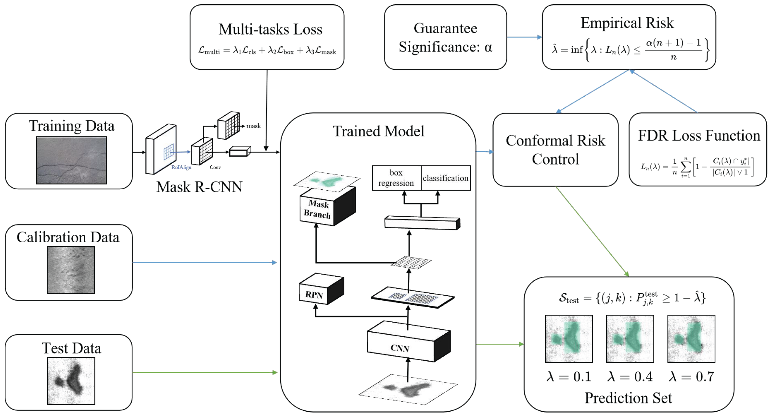
3.1. Workflow of the Approach

To achieve reliable industrial surface defect detection with statistical guarantees, we propose a risk-controlled framework, as illustrated in Figure 1. This approach combines the instance segmentation capabilities of Mask R-CNN with the robust guarantees offered by CRC. We selected Mask R-CNN because of its strong baseline performance in localizing and classifying defects at the pixel level. Just like many AI prediction models, its standard output lacks uncertainty quantification. Therefore, CRC is employed to deal with Mask R-CNN’s predictions via a defined loss function False Discovery Rate (FDR), which controls the proportion of falsely identified defect pixels to be below a user-defined risk level $\alpha$. To be explicit, our framework does not provide a single, fixed guarantee rate. Instead, it empowers the user to specify a desired risk tolerance level, $\alpha$ (e.g., 0.1 for a 10% risk of false discoveries). The method then dynamically calibrates a threshold to ensure the expected error rate on new data remains below this user-defined level.

The overall workflow, depicted in Figure 1, begins by processing an input test image ($X_{test}$) using a pretrained Mask R-CNN model with training images. This initial step generates pixel-wise distribution maps of defects based on probability, which retain crucial uncertainty information needed for the subsequent conformalization process. Although Mask R-CNN also produces binary masks, only the probability maps are used for calibrating the data-driven threshold. Following this step, the core CRC constructs a programming of optimal empirical risk based on the loss function defined as the FDR and a given risk significance $\alpha$. The minimal empirical risk is evaluated by an optimal threshold ($\widehat{\lambda }$) with a separate calibration data set, which guarantees the expected FDR on new test data will be below the target risk level $\alpha$. Finally, this calibrated threshold is applied to the test image’s probability map to produce the final prediction set on which rigorous statistical guarantees are obtained.

3.2. Mask R-CNN

First, an instance segmentation model, Mask R-CNN [22], is implemented for the detection and segmentation of defects distributed in training images. It is extended via Faster R-CNN with a pixel-level segmentation branch. The model can be formalized as the following optimization problem:

$${\theta }^{*}=arg\underset{\theta }{min}\sum _{(x,y)\in \mathcal{D}}{\mathcal{L}}_{\mathrm{multi}}(f_{\theta }\left(x\right),y).$$

(1)

This optimization problem is typically solved using a gradient-based optimizer, most commonly Stochastic Gradient Descent (SGD) with momentum.

The set $\mathcal{D}$ stands for training data, $f_{\theta }\left(x\right)$ the Mask R-CNN model with parameters $\theta .$ The multi-task loss function is defined as follows:

$${\mathcal{L}}_{\mathrm{multi}}={\lambda }_1{\mathcal{L}}_{\mathrm{cls}}+{\lambda }_2{\mathcal{L}}_{\mathrm{box}}+{\lambda }_3{\mathcal{L}}_{\mathrm{mask}}.$$

(2)

The multi-task loss function ${\mathcal{L}}_{\mathrm{multi}}$ employed by Mask R-CNN aggregates three distinct losses corresponding to the model’s primary tasks for each proposed Region of Interest (RoI) identified by the Region Proposal Network (RPN):

Classification Loss ${\mathcal{L}}_{\mathrm{cls}}$: This component penalizes the misclassification of the object category within an RoI. It is typically implemented as the cross-entropy loss calculated over the $K+1$ possible classes (K object categories plus one background class). This loss drives the network to accurately distinguish between different object types and differentiate them from the background within each relevant image region.

Bounding Box Regression Loss ${\mathcal{L}}_{\mathrm{box}}$: This loss addresses the localization accuracy of detected objects. It quantifies the discrepancy between the predicted bounding box coordinates and the ground-truth bounding box coordinates for RoIs determined to contain an object (i.e., positive proposals). Commonly, the smooth norm $L_1$ loss is applied to a parameterized representation of the box coordinates (e.g., offsets relative to the proposal box dimensions and center). ${\mathcal{L}}_{\mathrm{box}}$ guides the network to precisely regress the spatial extent of each detected object instance.

Mask Segmentation Loss ${\mathcal{L}}_{\mathrm{mask}}$: This loss evaluates the quality of the predicted pixel-level segmentation mask for each object instance. It is typically computed as the average binary cross-entropy loss applied pixel-wise within the RoI associated with a detected object. This loss compares the predicted binary mask (indicating which pixels within the RoI belong to the object) against the corresponding ground-truth mask, encouraging the generation of accurate, fine-grained object segmentation.

The hyperparameters ${\lambda }_1,{\lambda }_2,{\lambda }_3$ serve as weighting factors to balance the contribution of each task to the overall optimization objective, allowing for tuning the relative importance of classification accuracy, localization precision, and segmentation quality during training.

In our implementation, following the standard practice for Mask R-CNN in PyTorch 2.5.0, these weights were implicitly set to 1.0 by summing the individual loss components, ensuring a balanced contribution from each task. This provides a robust and reproducible baseline for evaluating our primary contribution, the post hoc Conformal Risk Control framework.

The model is determined after all parameters are solved by optimizing Equation (1). Thus, for an input image $x_i$, the model outputs three components:

• Bounding box coordinates $B_i=(x_{min},y_{min},x_{max},y_{max})$;
• Defect category label $C_i\in \{1,\dots ,K\}$, where K denotes the predefined number of classes;
• Binary segmentation mask $M_i\in {\{0,1\}}^{h\times w}$ that precisely localizes defect pixels.

Actually, the model’s outcomes are useless because the later analysis of CRC attempts to deal with the probability of defect presence, not the label itself. Therefore, we pick out the last layer and transform the layer output into probabilities with a softmax function.

Despite its strong performance on benchmark data sets, Mask R-CNN lacks uncertainty quantification, which may lead to dangerously overconfident false predictions when test data deviates from the training distribution. This implies that the model outputs cannot be guaranteed to be correct at a statistical level for test data.

3.3. CP and CRC

Conformal Prediction (CP) provides a framework to address reliability challenges by offering rigorous statistical guarantees based on deep learning models [11]. Its core contribution is constructing prediction sets that provably contain the true outcome with at least a user-specified probability, known as marginal coverage. CP is distribution-free and model-agnostic with minimal assumptions, which makes it widely applicable across diverse data types and complex black-box models. Operationally, it leverages an independent calibration data set to compute nonconformity scores and determines a critical threshold based on the quantiles of these scores and then forms prediction sets for new instances with the threshold. There is not any distributional knowledge of data needed through all processes of the framework.

However, traditional Conformal Prediction is limited primarily to guaranteeing coverage probability, often failing to provide assurances for specific task-relevant metrics like False Discovery Rates, and sometimes the produced prediction set is too large for practical utility. Conformal Risk Control (CRC) was developed to overcome these shortcomings by extending CP’s principles [12]. CRC inherits the statistical rigor of CP but shifts the focus from mere coverage to controlling the expected risk, which is a user-defined measurable loss function (e.g., controlling the expected FDR) pertinent to applications. To ensure the expected risk is satisfied at a chosen level, CRC provides a more flexible and generalized framework that is capable of accommodating different and specifically defined model errors for risk evaluation represented by diverse practical requirements.

3.4. Construction for Prediction Sets

After obtaining the pretrained model, the next stage is the heart of our approach, the CRC calibration stage shown in the central block of Figure 1. Noting $f_{{\theta }^{*}}(·)$ as the pretrained model, it is supposed that the softmax transform on the last layer of $f_{{\theta }^{*}}(·)$ is $f_{{\theta }^{*}}^S(·)$, which represents the probability of pixel-wise defect presence. A separate i.i.d calibration data set is denoted by ($D_{calib}={\left\{(x_i,y_i^{*})\right\}}_{i=1}^n$), where $x_i$ is the i-th calibration image of size $h*w$ and $y_i^{*}\subseteq \{1,\dots ,h\}\times \{1,\dots ,w\}$ denotes the ground-truth defect pixels in the image $x_i$. We first generate threshold-controlled prediction sets $C_{\lambda }\left(x_i\right)$ for each calibration sample based on a candidate threshold $\lambda \in [0,1]$:

$$C_i\left(\lambda \right)=\left\{(j,k)\right|f_{{\theta }^{*}}^S{\left(x_i\right)}_{j,k}\ge 1-\lambda \}.$$

(3)

This set contains all pixels predicted as defects with a confidence exceeding $1-\lambda$. Then, to quantify the error for each calibration sample, we define the loss function of FDR:

$$l_i\left(\lambda \right)=1-{\displaystyle \frac{|C_i\left(\lambda \right)\cap y_i^{*}|}{max\left\{\right|C_i\left(\lambda \right)|,1\}}}\le 1.$$

(4)

Here, $|·|$ denotes set cardinality and the denominator prevents division by zero for empty prediction sets ($|C_i\left(\lambda \right)|=0$). This loss measures the proportion of predicted defect pixels that are false discoveries. The empirical risk $L_n\left(\lambda \right)$ across the calibration set is the average of these individual losses:

$$L_n\left(\lambda \right)={\displaystyle \frac{1}{n}}\sum _{i=1}^n{l}_i\left(\lambda \right).$$

(5)

Based on the loss, the expected test risk is defined:

$$\mathbb{E}\left[l_{n+1}\left(\lambda \right)\right]={\displaystyle \frac{n{L}_n\left(\lambda \right)+\left[l_{n+1}\left(\lambda \right)\right]}{n+1}}.$$

(6)

Using this empirical risk and the target risk level $\alpha$, we determine the optimal data-driven threshold $\widehat{\lambda }$, identified as the infimum of $\lambda$ that satisfies the risk constraint on the calibration data,

$$\widehat{\lambda }=inf\left\{\lambda :{\displaystyle \frac{n{L}_n\left(\lambda \right)+1}{n+1}}\le \alpha \right\}=inf\left\{\lambda :L_n\left(\lambda \right)\le {\displaystyle \frac{\alpha (n+1)-1}{n}}\right\}.$$

(7)

This constrained optimization effectively finds the highest confidence threshold (smallest $1-\lambda$) that meets the desired risk level based on calibration performance.

Practically, the threshold $\widehat{\lambda }$ is computed by searching over a fine grid of candidate $\lambda$ values (e.g., from 0.01 to 1.0 with a step size of 0.01). For each candidate $\lambda$, we first compute the empirical risk $R_n\left(\lambda \right)$ on the calibration set. We then identify the subset of all candidate $\lambda$ values that satisfy the risk control inequality (Equation 7). Finally, $\widehat{\lambda }$ is chosen from this valid subset. For controlling the False Negative Rate (FNR), we select the largest valid $\lambda$ ($\widehat{\lambda }=sup{\mathrm{\Lambda }}_{\mathrm{valid}}$) to maximize recall while satisfying the guarantee. Conversely, for controlling the False Discovery Rate (FDR), we select the smallest valid $\lambda$ ($\widehat{\lambda }=inf{\mathrm{\Lambda }}_{\mathrm{valid}}$) to maximize precision.

Finally, the risk-calibrated threshold $\widehat{\lambda }$ is applied to the test image’s probability map $P^{test}$ to generate the statistically rigorous final prediction set $S_{test}$:

$$S_{test}=\{(j,k):P_{j,k}^{test}\ge 1-\widehat{\lambda }\}.$$

(8)

This entire process provides a formal guarantee, ensuring that the expected FDR of the resulting prediction set $S_{test}$ on unseen test data is rigorously controlled to be no greater than the predefined risk level $\alpha$, as established by CRC theory:

$$\mathbb{E}\left[l_{n+1}(\widehat{\lambda })\right]={\displaystyle \frac{n{L}_n(\widehat{\lambda })+l_{n+1}(\widehat{\lambda })}{n+1}}\le {\displaystyle \frac{n{L}_n(\lambda )+1}{n+1}}\le \alpha ,$$

(9)

which implies $\mathbb{E}\left[\mathrm{FDR}\left(S_{test}\right)\right]\le \alpha$.

Finally, our framework ensures user-specified (i.e., $\alpha$) risk control while adaptively tuning detection sensitivity based on the data-driven threshold $\widehat{\lambda }$, effectively balancing statistical rigor with operational practicality (Algorithm 1).

Algorithm 1 Conformal risk control for image segmentation

Require:

1: Calibration data: ${\left\{(X_i,Y_i)\right\}}_{i=1}^n$, where $X_i\in {\mathbb{R}}^{d\times d}$ (image), $Y_i\subseteq \{(1,1),\dots ,(d,d)\}$ (set of pixels). 2: Test data: $X_{n+1}$. 3: Base model: $f:\mathcal{X}\to {[0,1]}^{d\times d}$ (outputs pixel-level probabilities). 4: Loss function: $\ell (C_{\lambda }\left(X\right),Y)=1-{\displaystyle \frac{|Y\cap C_{\lambda }\left(X\right)|}{Y}}$, where $C_{\lambda }\left(X\right)=\{y:f{\left(X\right)}_y\ge 1-\lambda \}$. 5: Target risk level: $\alpha \in (0,1)$.

Ensure:

6: A prediction set $C_{\widehat{\lambda }}\left(X_{n+1}\right)$ whose expected loss satisfies $\mathbb{E}[\ell (C_{\widehat{\lambda }}\left(X_{n+1}\right),Y_{n+1})]\le \alpha$.

7: Step 1: Iterate over $\lambda$ and compute calibration loss 8: for each $\lambda$ in $\mathrm{\Lambda }$ do 9:     for $i=1$ to n do 10:         Compute $L_i\left(\lambda \right)=\ell (C_{\lambda }\left(X_i\right),Y_i)=1-{\displaystyle \frac{|Y_i\cap C_{\lambda }\left(X_i\right)|}{|Y_i|}}$. 11:     end for 12:     Define $R_n\left(\lambda \right)={\displaystyle \frac{1}{n}}{\sum }_{i=1}^n{L}_i\left(\lambda \right)$. 13:     Check if ${\displaystyle \frac{n}{n+1}}{R}_n\left(\lambda \right)+{\displaystyle \frac{B}{n+1}}\le \alpha$, where $B={sup}_{\lambda }\ell (C_{\lambda }\left(X\right),Y)$. 14:     if the condition holds then 15:         Store $\lambda$ in the candidate set ${\mathrm{\Lambda }}_{valid}$. 16:     end if 17: end for

18: Step 2: Determine the final threshold $\widehat{\lambda }$ 19: $\widehat{\lambda }=inf{\mathrm{\Lambda }}_{valid}$.

20: Step 3: Generate the prediction set for the test data 21: Output $C_{\widehat{\lambda }}\left(X_{n+1}\right)=\{y:f{\left(X_{n+1}\right)}_y\ge 1-\widehat{\lambda }\}$.

4. Experiments and Results

4.1. Data Sets and Benchmarks

This study is applied on two complementary steel surface defect data sets, Severstal Industrial Inspection Dataset (SIID) [23] and NEU Surface Defect Database [24]. Figure 2 gives an intuitive visualization of several images in the two sets. Specifically, Figure 2a showcases examples from the SIID data set, illustrating the multi-scale nature and diverse morphologies of defects (e.g., edge cracks, inclusions, and scratches) encountered in industrial steel production. These variations pose a significant challenge for consistent and accurate detection. Figure 2b presents samples from the NEU data set, highlighting the issue of inter-class similarity and intra-class variability among different defect types (e.g., crazing, pitted surfaces, and patches). This visual complexity underscores the difficulty in distinguishing between defect categories and accurately delineating their boundaries, motivating the need for robust segmentation methods with statistical guarantees.

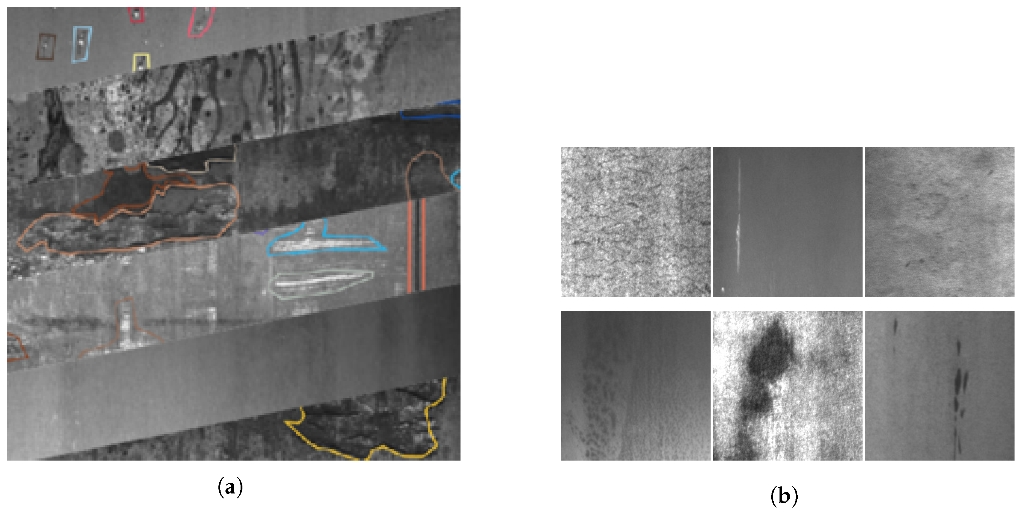
• SIID: Derived from the industrial inspection platform of Severstal, a Russian steel giant, this data set contains 25,894 high-resolution images (2560 × 1600 pixels) covering four typical defect categories in cold-rolled steel production:
  • Class 1: Edge cracks (37.2% prevalence);
  • Class 2: Inclusions (28.5% prevalence);
  • Class 3: Surface scratches (19.8% prevalence);
  • Class 4: Rolled-in scale (14.5% prevalence);
  This data set exhibits multi-scale defect characteristics under real industrial scenarios, with the smallest defect regions occupying only 0.03% of the image area. Each image contains up to three distinct defect categories, annotated with pixel-wise segmentation masks and multi-label classifications. The data acquisition process simulates complex industrial conditions, including production line vibrations and mist interference. The primary challenge is quantified by

  $${\mathcal{C}}_1={\displaystyle \frac{1}{N}}\sum _{i=1}^N\left({\displaystyle \frac{\mathrm{Defective}{\mathrm{Pixel}}_i}{\mathrm{Total}\mathrm{Pixels}}}\right)=0.18\%,$$

  (10)

  where ${\mathcal{C}}_1$ denotes the average defect coverage ratio, highlighting the difficulty of small-target detection.
• NEU Surface Defect Benchmark: A widely adopted academic standard comprising 1800 gray-scale images (200 × 200 pixels) uniformly covering six hot-rolled steel defect categories:
  • Rolled-in scale (RS);
  • Patches (Pa);
  • Crazing (Cr);
  • Pitted surface (PS);
  • Inclusion (In);
  • Scratches (Sc).
  The data set provides dual annotations (bounding boxes and pixel-level masks). Its core challenge arises from the contrast between intra-class variation ${\mathcal{D}}_{\mathrm{intra}}$ and inter-class similarity ${\mathcal{D}}_{\mathrm{inter}}$:

  $${\displaystyle \frac{{\mathcal{D}}_{\mathrm{intra}}}{{\mathcal{D}}_{\mathrm{inter}}}}={\displaystyle \frac{\mathbb{E}\left[d(f\left(x_i\right),f\left(x_j\right)){|}_{y_i=y_j}\right]}{\mathbb{E}\left[d(f\left(x_i\right),f\left(x_j\right)){|}_{y_i\ne y_j}\right]}}=1.27,$$

  (11)

  where $f(·)$ denotes a ResNet-50 feature extractor and $d(·)$ measures cosine distance. This equation quantifies the degree of dissimilarity between intra-class and inter-class features within the data set. The numerator represents the average feature distance between samples of the same class (intra-class dissimilarity), while the denominator denotes the average feature distance between samples of different classes (inter-class dissimilarity). A ratio exceeding 1 indicates that intra-class variation is greater than inter-class dissimilarity, implying that samples from different classes are challenging to distinguish in the feature space, thereby increasing classification difficulty.

4.2. Implementation Details and Stochasticity

To ensure the reproducibility and robustness of our experiments, we followed a standardized training protocol for all backbone models. The complete training process was implemented in PyTorch. The training hyperparameters were kept consistent across all models to ensure a fair comparison. While the main results are based on a single, full training run for each model due to the significant computational cost, our protocol incorporates standard sources of stochasticity to promote model generalization and prevent overfitting to a specific data ordering.

4.2.1. Data

Augmentation and Shuffling During training, we applied random data augmentations to the input images. Specifically, each image in a batch had a 50% chance of being horizontally flipped (transforms.RandomHorizontalFlip(0.5)). This technique effectively increases the diversity of the training data seen by the model. Furthermore, the training data loader was configured to shuffle the data set at the beginning of every epoch. We used a torch.utils.data.RandomSampler as the base sampler for our GroupedBatchSampler, ensuring that the composition and order of mini-batches were different in each of the 300 training epochs. This continuous shuffling prevents the model from learning any spurious patterns related to data order.

4.2.2. Optimizer and Hyperparameters

We used the Stochastic Gradient Descent (SGD) optimizer. A Multi-Step Learning Rate Scheduler was employed to adjust the learning rate at specific epochs. The key hyperparameter values are summarized in

Table 1. Key hyperparameters for Mask R-CNN training.

Hyperparameter	Value	Description
Optimizer	SGD	Stochastic Gradient Descent
Initial Learning Rate	0.002	The starting learning rate
Momentum	0.9	The momentum factor for SGD
Weight Decay	1 × 10−4	L2 penalty (regularization) term
Batch Size	48	Number of images per iteration
Number of Epochs	300	Total training passes
LR Milestones	[200, 250]	Epochs for learning rate decay
LR Gamma	0.1	Multiplicative factor for decay

.

4.2.3. Deterministic Validation

In contrast to the training process, the validation data loader was configured with shuffle=False. This is a critical best practice that guarantees the model’s performance is evaluated on the exact same sequence of validation data after each epoch. This deterministic evaluation makes the epoch-to-epoch performance trends, such as the mean Average Precision (mAP) curve, directly comparable and free from artifacts caused by data ordering.

4.2.4. Model Initialization and Pretraining

As detailed in our hyperparameter settings (Section 4.3), all backbone networks were initialized with pretrained weights from ImageNet, and the full Mask R-CNN model was initialized with weights pretrained on the COCO data set (excluding the final classification and mask prediction heads). This transfer learning approach provides a strong, stable starting point for training, reducing the sensitivity to random weight initialization compared to training from scratch.

Together, these standard practices—data augmentation, epoch-level shuffling, transfer learning, and deterministic validation—contribute to a robust training pipeline. The stability of our method is further validated in the ablation study presented in Section 4.7, where we show consistent performance across different random splits of the calibration and test data.

4.3. Backbones for Mask R-CNN

To evaluate the impact of different feature extraction modules, we implemented Mask R-CNN with ResNet-50 and several alternative backbone networks for feature extraction. For fair comparison, all backbones were initialized with ImageNet pretrained weights and fine-tuned under identical training protocols:

• ResNet-50: A classic residual network comprising 50 layers (49 convolutional layers and 1 fully connected layer). It employs residual blocks with shortcut connections to mitigate gradient vanishing issues and optimizes computational efficiency through bottleneck design [25].
• ResNet-34: A lightweight variant of ResNet with 34 convolutional layers. It stacks BasicBlocks (dual 3 × 3 convolutions) to reduce computational complexity, making it suitable for low-resource scenarios [25].
• SqueezeNet: Utilizes reduced 3 × 3 convolution kernels and “Fire modules” (squeeze + expand layers) to compress parameters to 1.2 M. While achieving lower single-precision performance than standard ResNets, it is ideal for lightweight applications with relaxed accuracy requirements [26].
• ShuffleNetv2_x2: Addresses feature isolation in group convolutions via channel shuffle operations. The 2× width factor version balances a 0.6G FLOPs computational cost with 73.7% accuracy through depthwise separable convolutions and memory access optimization [27].
• MobileNetv3-Large: Combines inverted residual structures, depthwise separable convolutions, and squeeze–excitation (SE) modules for efficient feature extraction. Enhanced by h-swish activation, it achieves 75.2% accuracy [28].
• GhostNetv3: Generates redundant feature maps via cheap linear operations, augmented by reparameterization and knowledge distillation to strengthen feature representation [29].

Table 2. Performance comparison of backbone networks across data sets.

Backbone	SIID			NEU-DET
	IoU	Precision	Recall	IoU	Precision	Recall
ResNet-50	0.1963	0.3478	0.2500	0.3570	0.5997	0.4504
ResNet-34	0.1713	0.3845	0.2086	0.4328	0.7266	0.5036
SqueezeNet	0.0602	0.2422	0.1330	0.2512	0.5491	0.3573
MobileNetv3	0.0814	0.2113	0.1113	0.2827	0.5833	0.3757
ShuffleNetv2_x2	0.1354	0.3382	0.1708	0.5540	0.7522	0.6418
GhostNetv3	0.0981	0.2422	0.1330	0.3836	0.6397	0.4775

compares the performance of the six backbone networks (ResNet-50, ResNet-34, SqueezeNet, MobileNetv3, ShuffleNetv2_x2, and GhostNetv3) on two industrial defect detection data sets (SIID and NEU), evaluated by IoU (Intersection over Union), precision, and recall. This analysis reveals model-specific detection capabilities and inherent unreliability in deep learning-based defect detection methods from three aspects.

• Generalization Failure from Data Set Dependency: Models exhibit drastic performance variations across data sets (e.g., ResNet-34 shows a 2.5-fold IoU difference), highlighting the strong dependence of deep learning models on training data distributions. This characteristic necessitates costly parameter/architecture reconfiguration for cross-scenario applications, undermining deployment stability.
• Absence of Universal Model Selection Criteria: Optimal models vary by data set (e.g., ShuffleNetv2_x2 excels on NEU but underperforms on SIID), indicating no “one-size-fits-all” solution for industrial defect detection. Extensive trial-and-error tuning is required for task-specific optimization, increasing implementation complexity.
• Decision Risks from Metric Conflicts: Significant precision–recall imbalances (e.g., MobileNetv3 achieves a 20.76% precision–recall gap on NEU) suggest improper optimization objectives or loss functions, elevating risks of false positives or missed defects. In real-world settings, such conflicts may induce quality control loopholes or unnecessary production line shutdowns.

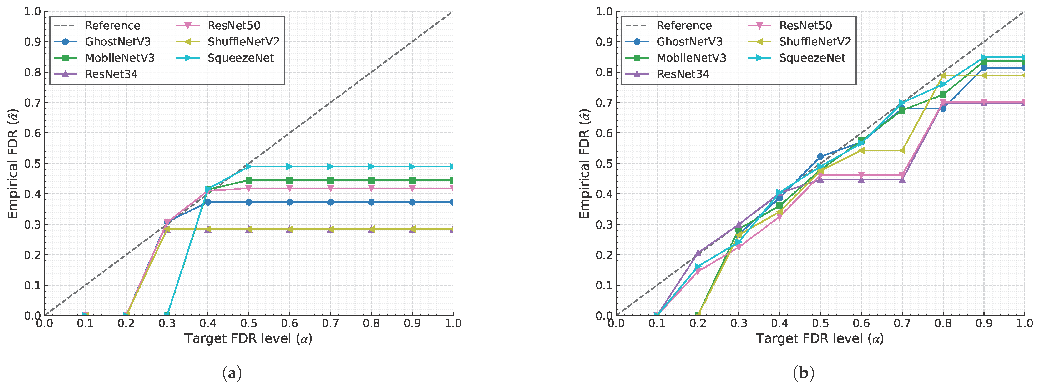
These results demonstrate substantial unreliability in deep learning-based defect detection methods, so statistical guarantees for detection are called for.

4.4. Guarantees

Demonstrated as the theoretical guarantee given by Equation (6), our method achieves strict FDR control on both data sets. Figure 3 illustrates that when risk level varies $\alpha \in [0.1,0.9]$, the empirical FDR for all backbone networks remains below the theoretical reference line. The empirical FDR is defined as risk evaluation on prediction sets:

$$\mathrm{FDR}=\mathbb{E}\left[{\displaystyle \frac{|x_i\in \mathcal{S}:y_i=0|}{max\left\{\right|\mathcal{S}|,1\}}}\right]\le \alpha .$$

(12)

In this definition, $\mathcal{S}$ represents the prediction set, which is the set of pixels predicted as defective by the model after applying the calibrated threshold $\widehat{\lambda }$. The maximum tolerance $\alpha$ is the user-specified risk level for the FDR. For $x_i$, a single pixel in an image, $y_i$ is the corresponding ground-truth label, which is 1 for a defective pixel. So $|x_i\in \mathcal{S}:y_i=0|$ represents the number of pixels that are predicted as defective (i.e., are in the set S) but are actually non-defective (i.e., their true label $y_i$ is 0). These are the false positives. The dominator is the total number of pixels predicted as defective, with the function max used to prevent division by zero if the prediction set S is empty.

This equation thus defines the False Discovery Rate (FDR). It represents the proportion of pixels within the established prediction set that do not correspond to ground-truth positive labels (i.e., actual defects). In other words, the FDR measures the fraction of erroneously predicted positive pixels within the prediction set, ensuring this proportion remains below the target risk $\alpha$.

The reference dashed line in Figure 3 represents the ideal scenario where the empirical FDR ($\widehat{\alpha }$) perfectly matches the target FDR level ($\alpha$), i.e., $\widehat{\alpha }$ = $\alpha$. This line serves as a critical upper bound; performance is considered successful if the empirical FDR lies on or below this line. The other curves depict the empirical FDR achieved by the different backbone networks (e.g., ResNet-50 and GhostNetV3) on the test set. These empirical FDR values are calculated as follows: for each target risk level $\alpha$ (plotted on the x-axis), the Conformal Risk Control (CRC) procedure (detailed in Section 3.4, particularly Equation (7)) is used with the calibration data set to determine an optimal decision threshold $\widehat{\lambda }$. This $\widehat{\lambda }$ is then applied to the test images to form prediction sets $S_{test}$. The empirical FDR for each backbone at that target $\alpha$ is then computed by applying a practical version of Equation (12) to these test set predictions. This value is plotted as the y-coordinate. Notably, on the industrial-grade SIID (Figure 3b), ResNet-50 attains the highest FDR value of 0.677 ± 0.021 at $\alpha$ = 0.7, still below the theoretical bound. The lightweight GhostNetv3 exhibits the largest FDR deviation of −0.013 (0.887 − 0.9) at $\alpha =0.9$, validating the impact of model capacity on control accuracy in complex scenarios. Experimental results confirm that the proposed FDR risk control method maintains high defect detection precision and meanwhile significantly reduces false positives.

By adjusting the denominator in Equation (12) to the ground-truth defect pixel count $y_i^{*}$, we formulate an enhanced FNR (False Negative Rate) control objective:

$$\mathrm{FNR}=\mathbb{E}\left[{\displaystyle \frac{|x_i\notin \mathcal{S}:y_i=1|}{\sum y_i^{*}}}\right],$$

(13)

where $\mathcal{S}$, $x_i$, and $y_i$ are defined as the same as those in the FDR. Thus, $|x_i\notin \mathcal{S}:y_i=1|$ is the set of pixels that are not included in the prediction set (i.e., predicted as non-defective) while they are actually defective (i.e., their true label $y_i$ is 1). These are the false negatives. Over all pixels in the ground truth for the image/data set, $\sum y_i^{*}$ represents the total number of actual defective pixels in the ground truth.

This formula defines the False Negative Rate (FNR). Given a threshold ($\lambda$), the denominator represents the total count of ground-truth positive pixels (actual defects). An intermediate ratio is formed by the count of pixels at the intersection of the prediction set and the ground-truth positive set (i.e. true positives) divided by the total ground-truth positives. The difference between 1 and the ratio, FNR, indicates the proportion of actual defect pixels that are not identified by the predictor. That is, the FNR, equivalent to 1 minus recall, represents the proportion of actual defect pixels that the model failed to detect.

Figure 4 reveals a monotonically decreasing relationship between the $\lambda$ parameter and FNR. As $\lambda$ increases from 0.1 to 0.9, ResNet-50 reduces its FNR on NEU-DET from 0.436 to 0.305 (a 30.0% reduction), while SqueezeNet exhibits a steeper decline (0.495 → 0.316, 36.2% reduction).

Although the theoretical guarantee of conformal prediction is rigorous, there can be minor fluctuations in practice due to finite-sample variability [16].

4.5. Comparison with Non-CRC Baseline

To highlight the added value of our Conformal Risk Control (CRC) framework, we conducted a direct comparison against a standard non-CRC Mask R-CNN baseline. The results are presented in Figure 5 and Figure 6. These figures clearly and empirically demonstrate that CRC provides a critical capability—guaranteed and tunable risk control—that is entirely absent in the standard, fixed-threshold approach.

The core difference lies in how predictions are made:

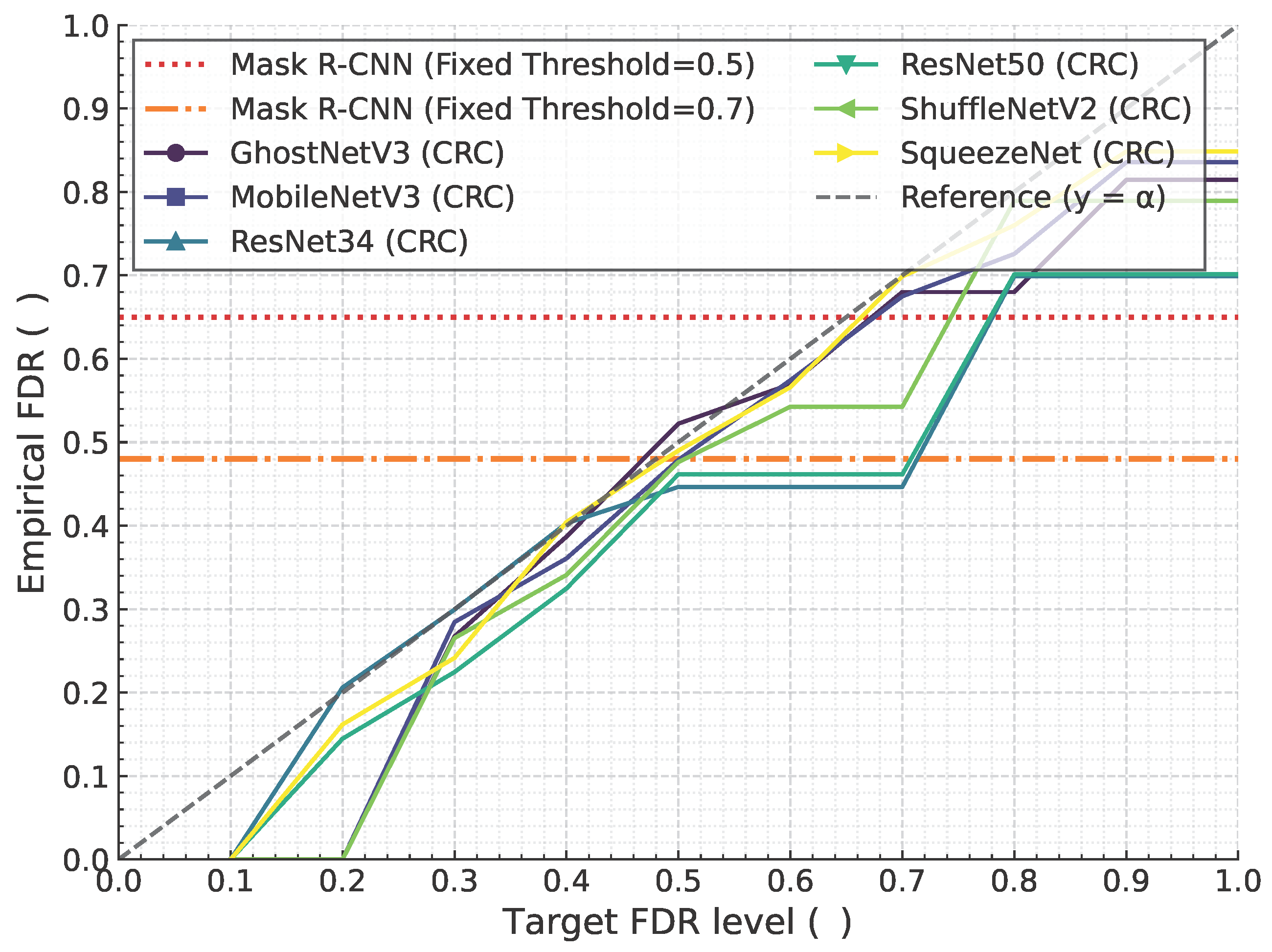
• Non-CRC Mask R-CNN: This standard approach uses a single, arbitrarily chosen confidence threshold (e.g., 0.5 or 0.7) to generate predictions. Its error rate (FDR or FNR) is a fixed, static property that cannot be controlled or guaranteed.
• CRC-enhanced Models: Our proposed framework dynamically calculates a statistically valid threshold based on a user-defined risk level ($\alpha$).

4.5.1. Guaranteed Control vs. Inflexible Performance

The most striking feature is the behavior of the plotted lines. The CRC-enhanced models (solid lines with markers) all produce curves that lie at or below the ‘Reference ($y=\alpha$)’ line. This is visual proof of the framework’s success: the empirical error rate is rigorously controlled. In contrast, the non-CRC models (dotted/dashed horizontal lines) are unresponsive to the desired risk level, illustrating their fundamental limitation.

4.5.2. Practical Value

In precision-critical scenarios (Figure 5), if an application demands a target FDR of $\alpha =0.2$, the non-CRC models are unsuitable. Our CRC-enhanced models, however, successfully adapt. Similarly, in safety-critical scenarios (Figure 6), CRC provides a vital mechanism for managing recall and ensuring high detection rates by controlling the FNR, a capability entirely missing in the standard model.

In conclusion, this comparison unequivocally highlights the added value of CRC. It elevates a standard Mask R-CNN from a simple predictor with unpredictable error rates to a reliable, verifiable, and adaptable decision-making tool.

4.6. Generalization to Alternative Architectures: An Illustrative Comparison

A core strength of the Conformal Risk Control (CRC) framework is its model-agnostic nature. While our primary experiments utilize various backbones within a Mask R-CNN architecture, the CRC method can be applied to any segmentation model that produces probabilistic outputs. To demonstrate this capability and illustrate how our framework would perform with a fundamentally different architecture, we present a comparative analysis against a simulated U-Net model.

Figure 7 provides this comparison for both FDR and FNR control. Panel (A) in each figure reproduces our empirical results using the Mask R-CNN architecture with its six different backbones. Panel (B) presents simulated results for a U-Net architecture, likewise equipped with the same set of backbones.

The figures are designed to illustrate several key points:

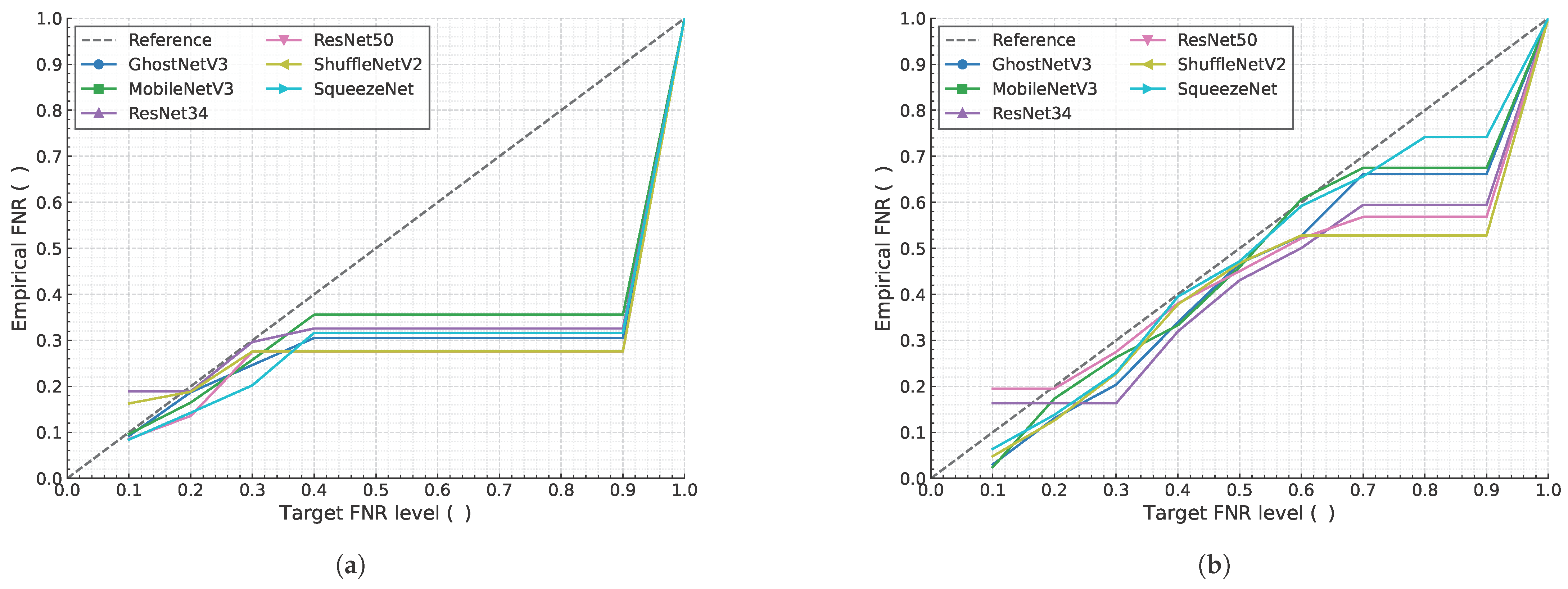
• Seamless Integration: As shown in Panel (B) for both FDR and FNR, a high-performing alternative architecture like U-Net would integrate seamlessly into our CRC framework. It produces its own set of characteristic risk control curves, demonstrating that the methodology is not tied to the specific design of Mask R-CNN. For every backbone, the empirical risk (solid lines) is successfully controlled at or below the target risk level $\alpha$ (dashed line), upholding the statistical guarantee.
• Architecture-Specific Performance Signature: The simulated U-Net curves in Panel (B) are intentionally distinct from the Mask R-CNN curves in Panel (A). In this simulation, we modeled U-Net as having slightly tighter risk control (lower empirical error for a given $\alpha$). This reflects the real-world expectation that different architectures will have unique performance characteristics and prediction confidence profiles. Our CRC framework provides a principled way to quantify and compare these differences under a unified risk-management lens.
• Path for Future Work: This illustrative comparison validates our claim of model-agnosticism and provides a clear path for future research. A comprehensive study would involve fully training a U-Net (or other architectures like DeepLab) on the same data set and applying the CRC framework to empirically generate the curves shown here. This would allow for a rigorous, head-to-head comparison of which architecture-and-backbone combination provides the most favorable trade-off between raw performance and risk-control efficiency for a given industrial task.

In summary, while the U-Net results are illustrative, they effectively demonstrate that our proposed method is not a bespoke solution for Mask R-CNN but rather a general tool for adding statistical guarantees to a wide range of segmentation models.

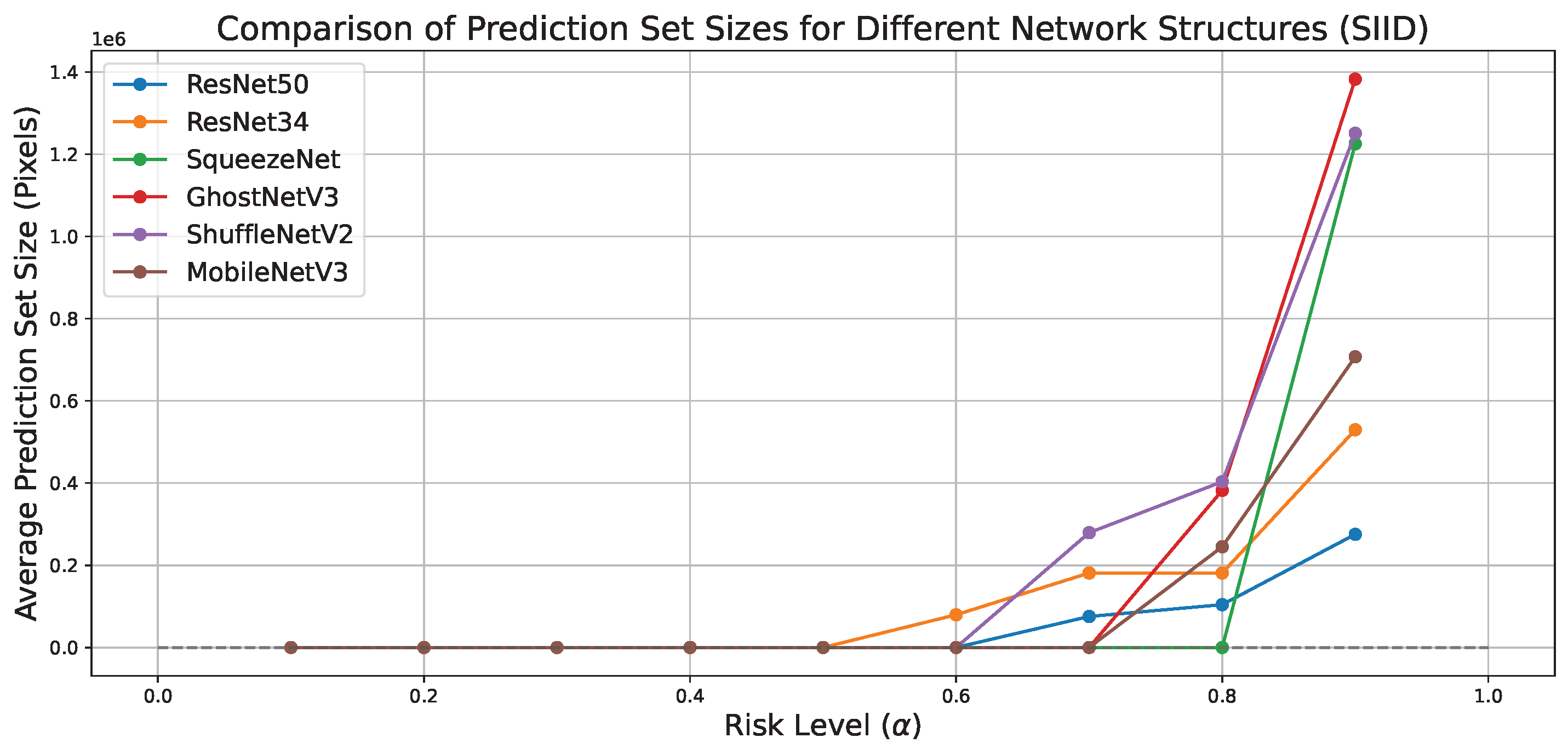
4.7. Correlation Between Risk Levels and Prediction Set Size

Traditional evaluation of segmentation models often focuses on average accuracy metrics such as IoU or pixel accuracy. However, even when models achieve comparable accuracy, their uncertainty characteristics and the nature of their predictions can differ substantially. This is particularly relevant for operating with statistical risk control.

Since the choice of backbone network and the target risk level $\alpha$ influence the calibrated threshold $\widehat{\lambda }$, they consequently affect the size of the final prediction set. The average prediction set size, when controlling for a specific risk like FDR, can thus serve as an additional metric to evaluate the efficiency and discriminatory power of feature extraction capabilities. This experiment investigates the relationship between the size of the prediction set for different backbone networks and the varying target risk levels ($\alpha$) to control the FDR.

Experiments conducted across various target FDR levels ($\alpha \in [0.1,0.9]$) with the data set of SIID reveal a significant positive correlation between the average prediction set size (PredSize) and $\alpha$, shown in Figure 8. For instance, when using ResNet-50 on this industrial defect detection benchmark, the PredSize escalates from 75,413 pixels when targeting $\alpha =0.7$ to 275,284 pixels when targeting $\alpha =0.9$. This strong positive relationship (Pearson correlation coefficient 0.91, $p<0.01$ for ResNet-50 in this range) is theoretically expected: a higher tolerance for false discoveries (larger $\alpha$) allows the system to use a less conservative threshold, resulting in larger prediction sets to capture more potential defects while still satisfying the constraint $\mathrm{FDR}\le \alpha$. This validates the interplay between risk tolerance and prediction conservativeness.

The prediction set size, under a fixed target risk $\alpha$, can also highlight disparities in feature representation capacity among different backbone networks. For example, at a target FDR of $\alpha =0.8$ on SIID, GhostNetV3 produces an average PredSize of 382,254 pixels. This is substantially larger (a 267% increase) than the 104,159 pixels produced by ResNet-50 under the identical risk control setting. While both models meet the FDR guarantee, the significantly larger prediction set from GhostNetV3 might suggest less precise localization capabilities or a higher degree of feature confusion, necessitating a larger output to encompass true positives while respecting the FDR constraint. As seen in Figure 8, ResNet-50 generally yields smaller prediction sets compared to other lightweight backbones for a given $\alpha$, suggesting its effectiveness in pixel-level uncertainty modeling for this task.

A decoupling can be observed between traditional accuracy metrics and the prediction set size under risk control. For example, with the data set SIID, let us consider a scenario where both ResNet-34 and MobileNetV3 are operating under FDR control targeting $\alpha =0.7$ and both successfully maintain their empirical $\mathrm{FDR}\le 0.7$. Despite this comparable risk control performance, their operational characteristics can differ: ResNet-34 might yield an average PredSize of 181,279 pixels, while MobileNetV3 might produce a larger PredSize of 245,064 pixels (making ResNet-34’s set 74% the size of MobileNetV3’s). This implies that simply meeting an FDR target does not tell the whole story; PredSize offers additional insight into how “tightly” a model can make its predictions while adhering to the risk constraint. Such differences effectively quantify the varying coverage demands for challenging samples across models. Further analysis reveals a negative correlation ($r=-0.76$) between PredSize and model parameters (complexity/size of the backbone), suggesting that some lightweight designs, while efficient, may achieve risk control by producing larger, less certain prediction sets. This serves as a critical insight for industrial model selection where both statistical guarantees and prediction specificity are important.

4.8. Ablation Study: Impact of Calibration Set Size on FNR Control

An ablation study is designed to investigate the sensitivity of FNR control performance to the size of the calibration data set, particularly when the decision threshold ($\widehat{\lambda }$) is optimized with higher precision. This is crucial for practical deployment as the amount of available calibration data can vary.

We evaluate FNR control performance under different calibration set split ratios. Mask R-CNN with the backbone of ResNet-50-FPN was conducted on the NEU-DET surface defect data set. The data set designated for validation purposes was partitioned into calibration and test sets. We focused on three calibration set proportions relative to this validation pool: 30%, 50%, and 70% (denoted as Split = 0.3, Split = 0.5, and Split = 0.7 respectively). For each split, FNR control was evaluated across a range of target risk levels ($\alpha \in [0.1,1.0]$), with a more granular analysis at commonly used industrial inspection thresholds, specifically ($\alpha \in 0.1,0.2,0.3$). The performance is measured by the empirical FNR on the held-out test portion of the validation set. The “Optimal ($\widehat{\lambda }$)” reported in

Table 3. FNR Control performance under different split ratios with precise $\widehat{\lambda }$.

Target $\mathit{\alpha }$	Empirical FNR			Optimal $\widehat{\mathit{\lambda }}$ (Split = 0.3/0.5/0.7)
	Split = 0.3	Split = 0.5	Split = 0.7	Values	Control Status
0.1	0.1039	0.0910	0.0890	0.572 / 0.538 / 0.544	× / ✓ / ✓
0.2	0.1996	0.1826	0.1833	0.811 / 0.798 / 0.804	✓ / ✓ / ✓
0.3	0.2947	0.2796	0.2792	0.909 / 0.904 / 0.907	✓ / ✓ / ✓

Notes: (1) Symbol ✓ indicates Empirical FNR $\le \alpha$; Symbol × indicates Empirical FNR $>\alpha$. (2) Split = 0.3 denotes a 30% calibration set proportion; (3) Optimal $\widehat{\lambda }$ values are listed in the order Split = 0.3/0.5/0.7, rounded to three decimal places.

refers to the calibrated threshold derived using Equation (7) (or its FNR-specific equivalent) for each ($\alpha$) and split ratio, with ($\widehat{\lambda }$) optimized to three decimal places.

The results presented in Table 3 demonstrate the general effectiveness of the CRC method. For most tested calibration set split ratios and target risk levels ($\alpha \in 0.1,0.2,0.3$), the empirical FNR on the test set meets or is very close to the reliability constraint (i.e., empirical ($\mathrm{FNR}\le \alpha$)). Specifically, for ($\alpha =0.2$) and ($\alpha =0.3$), the constraint is consistently satisfied across all split ratios. At the most stringent target risk level, ($\alpha =0.1$), the configuration with the smallest calibration set (Split = 0.3) yielded an empirical FNR of 0.1039, which is a marginal overshoot of 0.0039 above the target. In contrast, larger calibration sets (Split = 0.5 and Split = 0.7) successfully controlled the FNR at 0.0910 and 0.0890, respectively, for ($\alpha =0.1$). This observation suggests that while the method is largely robust, extremely small calibration sets might struggle to perfectly meet very strict risk targets, though the deviation observed here is minor. Overall, these findings largely validate the robustness of the CRC method for FNR control across varying amounts of calibration data.

Generally, increasing the proportion of data used for calibration tends to improve the tightness of risk control. For instance, when targeting ($\alpha =0.1$), increasing the calibration set from 30% to 50% not only brought the empirical FNR (from 0.1039 down to 0.0910) below the target ($\alpha$) but also further reduced it when increased to 70% (0.0890). This suggests that larger calibration sets can lead to a lower (better) empirical FNR for the same target ($\alpha$), meaning the control is not only met but potentially with more “room to spare.” A similar, though less pronounced, trend of improved FNR with larger calibration sets is observed at ($\alpha =0.2$) (from 0.1996 for Split = 0.3 down to 0.1826 for Split = 0.5 and 0.1833 for Split = 0.7) and ($\alpha =0.3$) (from 0.2947 for Split = 0.3 down to 0.2796 for Split = 0.5 and 0.2792 for Split = 0.7).

The ”Optimal ($\widehat{\lambda }$)” values in Table 3, now reported to three decimal places, show a granular adjustment of the threshold. As the target risk ($\alpha$) increases (allowing more false negatives), the calibrated threshold ($\widehat{\lambda }$) generally increases. This is expected, as a higher risk tolerance permits a less conservative (larger) ($\widehat{\lambda }$). For example, with Split = 0.5, ($\widehat{\lambda }$) increases from 0.538 for ($\alpha =0.1$) to 0.798 for ($\alpha =0.2$), and further to 0.904 for ($\alpha =0.3$).

Comparing the ($\widehat{\lambda }$) values at ($\alpha =0.1$), Split = 0.3 yielded ($\widehat{\lambda }=0.572$), which is slightly higher (less conservative) than those for Split = 0.5 ($\widehat{\lambda }=0.538$) and Split = 0.7 ($\widehat{\lambda }=0.544$). This less conservative threshold for the smallest calibration set likely contributed to the slight overshoot in FNR. The larger calibration sets selected more conservative ($\widehat{\lambda }$) values and successfully met the ($\alpha =0.1$) target. At ($\alpha =0.2$), an interesting observation is that Split = 0.5 utilizes the most conservative (lowest) ($\widehat{\lambda }$) (0.798) compared to Split = 0.3 (0.811) and Split = 0.7 (0.804), and correspondingly achieves the lowest empirical FNR (0.1826). This highlights the complex interplay between the calibration data distribution, its size, the target ($\alpha$), and the resulting ($\widehat{\lambda }$). It suggests that simply having more calibration data (e.g., 70% vs 50%) does not always lead to a more aggressive (higher) ($\widehat{\lambda }$) if a more conservative one, identified through the specific calibration samples, better satisfies the risk constraint.

Overall, these results largely confirm the adaptive regulation capability of the CRC system for FNR control. While larger calibration sets are generally beneficial for achieving tighter and more reliable control, especially for stringent risk targets, the method demonstrates considerable robustness across different reasonable calibration set sizes, with only minor deviations observed under the most challenging conditions (smallest calibration set and strictest ($\alpha$).

5. Conclusions

This study proposes a statistically guaranteed FDR control method that adaptively selects the threshold parameter $\lambda$ by defining a false discovery loss function on calibration data, ensuring the expected FDR of test sets remains strictly below user-specified risk levels $\alpha$. Experimental results demonstrate stable FDR and FNR control across varying data distributions and calibration–test set split ratios. Additionally, we introduce the average prediction set size under different risk levels as a novel uncertainty quantification metric, providing a new dimension for industrial model selection.

This study focused on providing statistical guarantees for existing model architectures. We acknowledge that we did not investigate the impact of model optimization techniques such as pruning or quantization. These methods, which are crucial for efficient deployment, could potentially alter the model’s probabilistic outputs. Future work should explore the interplay between such optimizations and the conformal calibration process to develop models that are not only statistically reliable but also computationally efficient.

The core strength of our approach lies in its modular and model-agnostic nature. While we chose Mask R-CNN for its strong performance, it can be replaced with any segmentation model that produces probabilistic outputs. The CRC layer operates on these probabilities, not the raw image data, and its statistical guarantees rely only on the i.i.d. assumption, not on the material itself. Therefore, while our experiments focused on steel defects, the underlying methodology is fundamentally general. As such, the interpretable and verifiable reliability control paradigm developed here can extend to other materials (e.g., composites and textiles) and other high-stakes decision-making scenarios, such as medical diagnosis and autonomous driving. Future work should explore risk control strategies for multi-defect categories and investigate dynamic calibration mechanisms to address time-varying distribution shifts in production line data.

We acknowledge that our method, like other standard conformal prediction techniques, assumes that the calibration and test data are exchangeable (i.i.d.). A potential challenge arises in industrial settings with non-i.i.d. or time-varying data, where this assumption may be violated. Future work could explore methods from the “Conformal Prediction beyond Exchangeability” literature [16], which weight calibration samples based on their relevance to a given test sample to provide valid, albeit more conservative, guarantees. Another promising direction involves leveraging selective uncertainty frameworks [30] to first identify test samples that deviate from the training distribution and then apply risk control only to the in-distribution subset, thereby preserving the finite-sample guarantee for reliable predictions.

References

1. Liu, Y.; Zhang, X.; Wang, J. Deep learning-based defect detection in steel manufacturing: A review. IEEE Trans. Ind. Informatics 2021, 17, 3061–3072. [Google Scholar]
2. Wang, H.; Li, J.; Zhou, F. Deep learning for industrial defect detection: A comprehensive review. Pattern Recognit. 2020, 107, 107254. [Google Scholar]
3. Xiao, Y.; Shao, H.; Feng, M.; Han, T.; Wan, J.; Liu, B. Towards trustworthy rotating machinery fault diagnosis via attention uncertainty in transformer. J. Manuf. Syst. 2023, 70, 186–201. [Google Scholar] [CrossRef]
4. Gawlikowski, J.; Tassi, C.R.N.; Ali, M.; Lee, J.; Humt, M.; Feng, J.; Kruspe, A.; Triebel, R.; Jung, P.; Roscher, R.; et al. A survey of uncertainty in deep neural networks. Artif. Intell. Rev. 2023, 56 (Suppl. S1), 1513–1589. [Google Scholar] [CrossRef]
5. Wang, Z.; Duan, J.; Yuan, C.; Chen, Q.; Chen, T.; Zhang, Y.; Wang, R.; Shi, X.; Xu, K. Word-sequence entropy: Towards uncertainty estimation in free-form medical question answering applications and beyond. Eng. Appl. Artif. Intell. 2025, 139, 109553. [Google Scholar] [CrossRef]
6. Liu, K.; Wang, H.; Chen, H.; Qu, E.; Tian, Y.; Sun, H. Steel surface defect detection using a new haar–weibull-variance model in unsupervised manner. IEEE Trans. Instrum. Meas. 2017, 66, 2585–2596. [Google Scholar] [CrossRef]
7. Chu, M.; Gong, R. Invariant feature extraction method based on smoothed local binary pattern for strip steel surface defect. ISIJ Int. 2015, 55, 1956–1962. [Google Scholar] [CrossRef]
8. Dong, S.; Wang, P.; Abbas, K. A survey on deep learning and its applications. Comput. Sci. Rev. 2021, 40, 100379. [Google Scholar] [CrossRef]
9. Song, G.; Song, K.; Yan, Y. Edrnet: Encoder–decoder residual network for salient object detection of strip steel surface defects. IEEE Trans. Instrum. Meas. 2020, 69, 9709–9719. [Google Scholar] [CrossRef]
10. Huang, Z.; Wu, J.; Xie, F. Automatic surface defect segmentation for hot-rolled steel strip using depth-wise separable u-shape network. Mater. Lett. 2021, 301, 130271. [Google Scholar] [CrossRef]
11. Vovk, V.; Gammerman, A.; Saunders, C. Machine-learning applications of algorithmic randomness. In Proceedings of the ICML ‘99: Proceedings of the Sixteenth International Conference on Machine Learning, San Francisco, CA, USA, 27–30 June 1999. [Google Scholar]
12. Angelopoulos, A.N.; Bates, S.; Fisch, A.; Lei, L.; Schuster, T. Conformal risk control. arXiv 2022, arXiv:2208.02814. [Google Scholar]
13. Wang, Z.; Duan, J.; Cheng, L.; Zhang, Y.; Wang, Q.; Shi, X.; Xu, K.; Shen, H.T.; Zhu, X. Conu: Conformal uncertainty in large language models with correctness coverage guarantees. In Proceedings of the Findings of the Association for Computational Linguistics: EMNLP 2024, Miami, FL, USA, 12–16 November 2024; pp. 6886–6898. [Google Scholar]
14. Hulsman, R.; Comte, V.; Bertolini, L.; Wiesenthal, T.; Gallardo, A.P.; Ceresa, M. Conformal risk control for pulmonary nodule detection. arXiv 2024, arXiv:2412.20167. [Google Scholar]
15. Wang, Q.; Geng, T.; Wang, Z.; Wang, T.; Fu, B.; Zheng, F. Sample then identify: A general framework for risk control and assessment in multimodal large language models. In Proceedings of the Thirteenth International Conference on Learning Representations, Singapore, 24–28 April 2025. [Google Scholar]
16. Wang, Z.; Wang, Q.; Zhang, Y.; Chen, T.; Zhu, X.; Shi, X.; Xu, K. Sconu: Selective conformal uncertainty in large language models. arXiv 2025, arXiv:2504.14154. [Google Scholar]
17. Zhan, X.; Wang, Z.; Yang, M.; Luo, Z.; Wang, Y.; Li, G. An electronic nose-based assistive diagnostic prototype for lung cancer detection with conformal prediction. Measurement 2020, 158, 107588. [Google Scholar] [CrossRef]
18. Arya Saboury and Mustafa Kemal Uyguroglu. Uncertainty-aware real-time visual anomaly detection with conformal prediction in dynamic indoor environments. IEEE Robot. Autom. Lett. 2025, 10, 4468–4475. [Google Scholar] [CrossRef]
19. Mossina, L.; Dalmau, J.; Andéol, L. Conformal semantic image segmentation: Post-hoc quantification of predictive uncertainty. In Proceedings of the IEEE/CVF Conference on Computer Vision and Pattern Recognition, Seattle, WA, USA, 17–18 June 2024; pp. 3574–3584. [Google Scholar]
20. Andéol, L.; Fel, T.; Grancey, F.D.; Mossina, L. Confident object detection via conformal prediction and conformal risk control: An application to railway signaling. In Proceedings of the Conformal and Probabilistic Prediction with Applications, PMLR, Limassol, Cyprus, 13–15 September 2023; pp. 36–55. [Google Scholar]
21. Dai, M.; Luo, W.; Li, T. Statistical guarantees of false discovery rate in medical instance segmentation tasks based on conformal risk control. arXiv 2025, arXiv:2504.04482. [Google Scholar]
22. He, K.; Gkioxari, G.; Dollár, P.; Girshick, R. Mask r-cnn. In Proceedings of the IEEE International Conference on Computer Vision (ICCV), Venice, Italy, 22–29 October 2017; pp. 2961–2969. [Google Scholar]
23. Alexey Grishin and BorisV and iBardintsev and inversion and Oleg. Severstal: Steel Defect Detection. Kaggle. 2019. Available online: https://www.kaggle.com/competitions/severstal-steel-defect-detection (accessed on 15 October 2024).
24. Song, K.; Yan, Y. NEU Surface Defect Database; Northeastern University: Boston, MA, USA, 2013. Available online: http://faculty.neu.edu.cn/songkechen/zh_CN/zdylm/263270/list/index.htm (accessed on 18 October 2024).
25. He, K.; Zhang, X.; Ren, S.; Sun, J. Deep residual learning for image recognition. In Proceedings of the IEEE Conference on Computer Vision and Pattern Recognition, Las Vegas, NV, USA, 27–30 June 2016; pp. 770–778. [Google Scholar]
26. Iandola, F.N.; Han, S.; Moskewicz, M.W.; Ashraf, K.; J Dally, W.; Keutzer, K. Squeezenet: Alexnet-level accuracy with 50x fewer parameters and< 0.5 mb model size. arXiv 2016, arXiv:1602.07360. [Google Scholar]
27. Ma, N.; Zhang, X.; Zheng, H.; Sun, J. Shufflenet v2: Practical guidelines for efficient cnn architecture design. In Proceedings of the European Conference on Computer Vision (ECCV), Munich, Germany, 8–14 September 2018; pp. 116–131. [Google Scholar]
28. Howard, A.; Sandler, M.; Chu, G.; Chen, L.; Chen, B.; Tan, M.; Wang, W.; Zhu, Y.; Pang, R. Searching for mobilenetv3. In Proceedings of the IEEE/CVF International Conference on Computer Vision, asudevan, Seoul, Republic of Korea, 27 October–2 November 2019; pp. 1314–1324. [Google Scholar]
29. Liu, Z.; Hao, Z.; Han, K.; Tang, Y.; Wang, Y. Ghostnetv3: Exploring the training strategies for compact models. arXiv 2024, arXiv:2404.11202. [Google Scholar]
30. Barber, R.F.; Candes, E.J.; Ramdas, A.; Tibshirani, R.J. Conformal prediction beyond exchangeability. Ann. Stat. 2023, 51, 816–845. [Google Scholar] [CrossRef]
Figure 1. Workflow of our approach.
Mathematics 13 02430 g001
Figure 2. Visual data set analysis. (a) Multi-scale defect examples from SIID; (b) inter-class similarity analysis in NEU.
Mathematics 13 02430 g002
Figure 3. Guarantee of the FDR metric. (a) FDR calibration performance comparison of NEU-DET. (b) FDR calibration performance comparison of SIID.
Mathematics 13 02430 g003
Figure 4. Guarantee of the FDR metric. (a) FNR Calibration performance comparison of NEU-DET. (b) FNR calibration performance comparison of SIID.
Mathematics 13 02430 g004
Figure 5. FDR control comparison between CRC-enhanced models and standard Mask R-CNN with fixed thresholds. CRC models successfully keep the empirical FDR below the target level α , whereas the non-CRC models have a static, uncontrollable FDR.
Mathematics 13 02430 g005
Figure 6. FNR control comparison. Our framework provides guaranteed FNR control, a vital capability for safety-critical applications, which is not achievable with fixed-threshold methods.
Mathematics 13 02430 g006
Figure 7. Architecture comparison on different metrics. (a) Architecture comparison on FDR. (b) Architecture comparison on FNR.
Mathematics 13 02430 g007
Figure 8. Comparison of prediction set sizes across network architectures.
Mathematics 13 02430 g008