Cross-Domain Transfer Learning Architecture for Microcalcification Cluster Detection Using the MEXBreast Multiresolution Mammography Dataset

Abstract

Microcalcification clusters (MCCs) are key indicators of breast cancer, with studies showing that approximately 50% of mammograms with MCCs confirm a cancer diagnosis. Early detection is critical, as it ensures a five-year survival rate of up to 99%. However, MCC detection remains challenging due to their features, such as small size, texture, shape, and impalpability. Convolutional neural networks (CNNs) offer a solution for MCC detection. Nevertheless, CNNs are typically trained on single-resolution images, limiting their generalizability across different image resolutions. We propose a CNN trained on digital mammograms with three common resolutions: 50, 70, and 100 $\mathsf{\mu }$m. The architecture processes individual 1 cm² patches extracted from the mammograms as input samples and includes a MobileNetV2 backbone, followed by a flattening layer, a dense layer, and a sigmoid activation function. This architecture was trained to detect MCCs using patches extracted from the INbreast database, which has a resolution of 70 $\mathsf{\mu }$m, and achieved an accuracy of 99.84%. We applied transfer learning (TL) and trained on 50, 70, and 100 $\mathsf{\mu }$m resolution patches from the MEXBreast database, achieving accuracies of 98.32%, 99.27%, and 89.17%, respectively. For comparison purposes, models trained from scratch, without leveraging knowledge from the pretrained model, achieved 96.07%, 99.20%, and 83.59% accuracy for 50, 70, and 100 $\mathsf{\mu }$m, respectively. Results demonstrate that TL improves MCC detection across resolutions by reusing pretrained knowledge.

1. Introduction

In 2022, breast cancer was the most frequently diagnosed cancer in women worldwide, with 2.30 million recorded cases. More than 666 thousand of these resulted in fatalities, representing 15.5% of all cancer-related deaths [1]. By 2040, this number is expected to reach 3.16 million cases [2].

Mammography is the most used technique for the early detection of breast cancer [3,4], and its use has contributed to reducing the mortality rate of the disease by up to 48% [5]. Comparisons between different breast imaging techniques have highlighted mammography as the most effective and cost-efficient breast examination option [6]. Furthermore, mammography is considered the gold standard for breast cancer detection in women over 40 years old [7].

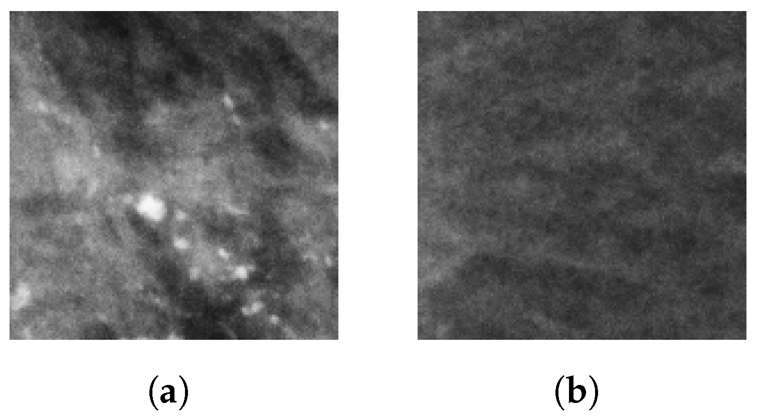
Microcalcifications (MCs) are the most significant indirect indicators of breast cancer. MCs appear as small deposits of calcium dots with diameters ranging from 0.1 mm to 1 mm and can be found either scattered or clustered along the mammary ducts [3,8]. In an X-ray image, MCs appear as pixel clusters that vary in brightness and contrast, and they can be dispersed or grouped in different regions of the breast [6,9].

MC detection is highly complex due to their size, shape, and distribution. Depending on their characteristics, it is possible to determine whether they are malignant or not at a high degree of accuracy. If diagnosed as malignant, a biopsy is mandatory for confirmation [10].

Groups of microcalcifications or microcalcification clusters (MCCs) describe situations where a set of MCs occupies a small portion of the breast tissue. This term is applied when at least three MCs are grouped within an area of 1 cm² [11,12,13]. MCCs are present in up to 50% of mammograms with confirmed cancer [12,13] and have a probability of malignancy ranging from 10% to 50%, which corresponds to the suspicious category with code 4 in the BI-RADS system [11].

Basile et al. [3] and Mordang et al. [14] highlighted that detecting MCCs represents a challenge, as they are imperceptible to touch. Therefore, imaging techniques are necessary for their detection. However, acquiring these images presents additional challenges, such as variability in breast composition, differences in texture, and low contrast.

The characteristics of mammograms vary according to the patient’s age and specific conditions, making MCC detection a complex challenge that can lead to misdiagnoses [15]. The early detection of MCCs, particularly in the initial stage of cancer, significantly increases survival rates. At this stage, the five-year survival rate reaches 99% [16].

Given the difficulty in detecting MCCs, caused by their small size, low contrast, variable appearance, and differences in breast tissue composition, researchers have explored artificial intelligence (AI) techniques to improve detection. Some studies have confirmed that using AI in medical imaging is safe and reliable [17]. Among the various AI techniques, deep learning (DL) has shown particularly promising results [18,19]. When trained with a large dataset, DL has achieved high levels of accuracy. DL architectures, such as convolutional neural networks (CNNs), are currently being studied for their effectiveness in detecting MCCs [3].

In the literature, several studies have demonstrated the high performance of CNNs in MCC detection. For instance, Wang et al. [13] developed a CNN for MCC detection using 521 screen-film mammography (SFM) images and 188 full-field digital mammography (FFDM) images, all collected by the Department of Radiology at the University of Chicago. The model achieved a 90% sensitivity, 0.69 false positives (FP) per image, and an area under the curve (AUC) of 0.971. Rehman et al. [15] designed a fully connected deep CNN (FC-DSCNN) for MCC detection and malignancy classification using 2885 SFM images from the Pakistan Institute of Nuclear Medicine and Radiotherapy (PINUM) dataset and 3568 SFM images from the Digital Database for Screening Mammography (DDSM). Although the original resolution is not specified, both datasets provide mammograms with a size of $320\times 240$ pixels, which suggests low spatial resolution. The model achieved a 99% sensitivity, 82% specificity, 2.45 FP per image, and 89% accuracy.

Hsieh et al. [10] used the VGG16 for MCC detection in mammograms, followed by an R-CNN to segment MCs within the detected MCCs and remove background noise. The InceptionV3 model was employed to classify the MCCs into benign or malignant. The model was trained and tested on 1,586 mammograms from a private dataset provided by the Department of Medical Imaging at the affiliated hospital of Chung-Shan Medical University. The study does not specify the image resolution or whether the mammograms are FFDM or SFM. The method achieved 93% and 95% accuracy in detection and segmentation, respectively, and 91% accuracy in malignancy classification. Overall, it reached 87% accuracy, 89% specificity, and 90% sensitivity.

Liu et al. [20] proposed a deep learning model to predict the malignancy of suspicious MCs, trained exclusively on patches extracted from craniocaudal (CC) and mediolateral oblique (MLO) mammographic views. The architecture consists of two MobileNetV2 networks, each trained on a specific view, sharing weights to extract features that are concatenated for malignancy prediction. The model was evaluated on a private dataset of 824 FFDM mammograms (CC and MLO views) corresponding to 414 BI-RADS 4 microcalcifications from 384 patients, acquired at Xinhua Hospital, Shanghai Jiao Tong University School of Medicine. The resolution and mammography system details were not reported. The image-based model achieved 76.5% sensitivity and 83.8% specificity on the test dataset.

Terrassin et al. [21] used ResNet-22, the ConvNeXt, and the UNet3+ CNNs to classify and segment malignant MCs in digital mammograms. The models were trained and evaluated on two public datasets: INbreast and the Breast Microcalcifications Dataset (BMCD), both annotated at the pixel level by expert radiologists. Although it is known that INbreast images were acquired at 70 $\mathsf{\mu }$m resolution, this detail was not reported in the article. The total number of mammograms was also not specified. They achieved an AUC of 0.93 for classification and 70% accuracy in segmentation.

Luna et al. [22] developed a residual shallow CNN for MCC detection. The model was trained and evaluated on 10 FFDM images from the INbreast dataset containing MCCs, achieving an accuracy of 99.71%. Additionally, when evaluated on the MEXBreast dataset at 70 $\mathsf{\mu }$m resolution, the same model reached 99.8% accuracy. In a comparative study using various CNN architectures trained and tested on the same INbreast subset, MobileNetV2 obtained the highest accuracy, with 99.84% [23].

Most studies, such as the previously mentioned ones, do not explicitly consider or report the mammograms’ resolution, primarily because they rely on publicly available datasets with varying resolutions and different acquisition technologies, implicitly assuming that CNNs can be trained without accounting for differences in image resolution and mammography type [24]. A summary of these studies and their dataset characteristics is provided in

Table 1. Comparison of studies using CNNs for the detection and classification of MCCs.

Study	Dataset	Modality	Resolution	Performance
[13]	Private	FFDM	Not specified	Sens: 90%, FP/img: 0.69, AUC: 0.971
[10]	Private	Not specified	Not specified	Sens: 90%, Spec: 89%, Acc: 87%
[15]	DDSM + PINUM	SFM	Not specified	Sens: 99%, Spec: 82%, FP/img: 2.45, Acc: 89%
[20]	Private	FFDM	Not specified	Sens: 76.5%, Spec: 83.8%
[21]	INbreast + BMCD	FFDM	70 $\mathsf{\mu }$m (INbreast)	Acc: 70%, AUC: 0.93
[23]	INbreast	FFDM	70 $\mathsf{\mu }$m	Acc: 99.84%
[22]	INbreast	FFDM	70 $\mathsf{\mu }$m	Acc: 99.71%
[22]	MEXBreast	FFDM	70 $\mathsf{\mu }$m	Acc: 99.8%

. Therefore, selecting an optimal image resolution may improve the performance of CNNs in radiology-based tasks. Hence, diagnostic tasks could benefit from higher image resolutions, as different pathologies may have varying resolution requirements for optimal detection. Whether variations in mammogram resolution across datasets affect the ability of CNNs to generalize effectively constitutes a research gap [25].

The performance of MCC detection algorithms is highly dependent on the database and the criteria by which the results are evaluated. This further emphasizes the need to carefully consider resolution variability when designing and assessing CNN models for MCC detection, as noted by Karale et al. [26]. Furthermore, the presence of both FFDM and SFM in available datasets introduces additional variability in resolution, since digital and film-based mammograms may exhibit different spatial characteristics. For instance, the images in the DDSM database were acquired using different scanners [27].

Table 2. Datasets and their corresponding resolutions and imaging modalities.

Dataset	Resolution ($\mathbf{\mu }$m)	Modality
DDSM	42, 43.5, 50	SFM [26,27]
CBIS-DDSM	42, 43.5, 50	SFM [28]
INbreast	70	FFDM [29]
OPTIMAM (OMI-DB)	50–100	FFDM & SFM [30]
BCDR	50	SFM [31]
MIAS	50	SFM [32]
MEXBreast	50, 70, 100	FFDM [33,34]

lists available mammography datasets and their corresponding resolutions and imaging modalities.

Due to the variability in mammogram resolution resulting from different acquisition scanners, it is important to assess whether CNN architectures can generalize across multiple resolutions. Although available mammography datasets provide valuable resources for MCC detection research, they exhibit variability in resolution and imaging modality, raising concerns about whether CNNs trained on a specific resolution can generalize effectively across different resolutions. Consequently, we propose a cross domain transfer learning (TL) architecture for MCC detection based on the MobileNetV2 architecture [35]. In a previous study [23], several CNN architectures were evaluated using the INbreast dataset at 70 $\mathsf{\mu }$m resolution, and the four best performing models were identified: VGG16, ResNet50, DenseNet121, and MobileNetV2. Among them, MobileNetV2 achieved the highest accuracy. To enable a fair comparison and assess the generalizability of these models, the same four architectures were trained from scratch using patches from our publicly available MEXBreast dataset [33,34] at the same resolution of 70 $\mathsf{\mu }$m, as described in Section 2.3. MobileNetV2 once again obtained the best performance, which supports its use in the present work.

We developed three new models adapted to 50 $\mathsf{\mu }$m, 70 $\mathsf{\mu }$m, and 100 $\mathsf{\mu }$m resolutions based on [23], following a feature extraction strategy. Their performance was then evaluated on independent mammography datasets to assess robustness across different imaging conditions.

The present study is driven by the need to address existing challenges, build upon previous advancements, and fill current gaps in the area. Specifically, most CNN-based approaches for MCC detection do not explicitly consider mammogram resolution, despite the variability introduced by different acquisition systems and imaging modalities. In addition, model performance often depends heavily on the characteristics of the datasets used, including whether they combine digital and film-based mammograms, which may differ in spatial quality. Finally, there is limited investigation into whether CNN models trained at one resolution can generalize to others, raising concerns about their robustness in heterogeneous clinical scenarios. By developing new methodologies that integrate the strengths of various techniques, current and future studies aim to improve the accuracy and reliability of early detection of breast lesions. Ultimately, these efforts contribute to developing AI models that can be integrated into devices to support more effective healthcare. The contributions of this paper are as follows:

• Feature extraction from the pretrained MobileNetV2: Features extracted from MobileNetV2, trained on 70 $\mathsf{\mu }$m resolution mammograms, were used to create three new models at 50 $\mathsf{\mu }$m, 70 $\mathsf{\mu }$m, and 100 $\mathsf{\mu }$m resolutions, improving detection performance on both lower and higher resolution images.
• A cross-domain CNN architecture for MCC detection with three different resolutions: A CNN architecture based on MobileNetV2 is proposed and trained from scratch to detect MCCs in mammograms at any of the three resolutions (50 $\mathsf{\mu }$m, 70 $\mathsf{\mu }$m, and 100 $\mathsf{\mu }$m), addressing the generalization limitations of training with single-resolution data.
• Demonstration of the superiority of TL across resolutions: Experimental results show that TL improves MCC detection accuracy compared to models trained from scratch, especially for non-native resolutions (98.32% vs. 96.07% for 50 $\mathsf{\mu }$m, 99.27% vs. 99.20% for 70 $\mathsf{\mu }$m, and 89.17% vs. 83.59% for 100 $\mathsf{\mu }$m).
• Efficient patch-based processing: The study introduces a consistent preprocessing method using 1 cm² patches, enabling scalable and resolution-consistent input handling across datasets.

The article is organized as follows: Section 2 describes the materials and methods; Section 3 presents the experimental setup and results; Section 4 discusses the findings; and Section 5 provides the conclusions and outlines future work.

2. Materials and Methods

This section presents an overview of the computational resources employed, the methods used for data acquisition, the training, validation and testing processes, and the architectural design of the CNN models for detecting MCCs.

2.1. Computational Resources

The experimentation was conducted using the Visual Studio Code 1.97.2 IDE with the Jupyter 2025.1.0 extension. The implementation was carried out in Python 3.9.6 with TensorFlow 2.16.2 and the TensorFlow Metal plugin.

The hardware setup consisted of a MacBook Pro with an Apple M4 Pro chip, featuring a 12-core CPU (4 performance and 8 efficiency cores), a 10-core GPU, a 16-core Neural Engine, 24 GB of unified memory, and a 500 GB Solid-State Drive (SSD).

2.2. Data Description

The mammogram patches used in this work were obtained from the MEXBreast database [33,34], a publicly available dataset created by our team. MEXBreast comprises 620 PNG mammograms annotated for MCCs by two expert radiologists [33,34]. The database includes 234 mammograms at a resolution of 50 $\mathsf{\mu }$m/pixel acquired with the Philips Sectra MicroDose L30 scanner, 462 mammograms at 70 $\mathsf{\mu }$m/pixel acquired with the Hologic Selenia Digital Mammography system, and 34 mammograms at 100 $\mathsf{\mu }$m/pixel acquired with the GE Senographe Essential scanner. The images are available in CC and MLO views for both the right and left breasts.

The dataset preparation followed a sequential process to ensure methodological consistency. First, patches were extracted according to their respective resolutions and class distributions. The datasets were split into training, validation, and testing subsets. Data augmentation techniques were subsequently applied only to the 100 $\mathsf{\mu }$m resolution, as it lacked a sufficient number of samples. Augmented versions of the same patch were restricted to a single subset to prevent data leakage and preserve integrity throughout the experiments.

2.2.1. Patch Extraction

The input to the proposed CNN models consists of mammogram patches of 1 cm² as this is the size of an MCC [12]. The patch dimensions depend on the mammogram resolution: $200\times 200$ pixels at 50 µm/pixel, $144\times 144$ pixels at 70 µm/pixel, and $100\times 100$ pixels at 100 µm/pixel.

The patches were categorized into two classes: class 1 for those with the presence of MCCs, and class 0 for those with the absence of MCCs. The procedure for extracting class 1 patches is described as follows:

1.

Localization of MCCs:

• The MCCs in the mammograms are identified using the coordinates $(X_1,Y_1)$ and $(X_2,Y_2)$ labeled by the expert radiologists and stored in the data file from the MEXBreast database [33,34].

2.

Definition of the extraction window:

• A sliding window of 1 cm² is used to traverse the region defined by the MCC coordinates.

3.

Patch extraction in four different directions:

• The window extracts a patch at each step of the sliding process. Four combined directions are used to increase variability: left to right and top to bottom, right to left and top to bottom, left to right and bottom to top, and right to left and bottom to top.

4.

Storage of patches:

• Each extracted patch are saved into a database for further analysis.

5.

Duplicate removal:

• The extracted patches are verified to ensure that there are no duplicates. Any redundant patch cut during the sliding process is removed.

The size of an MC typically ranges from 0.1 mm to 1 mm [3]. The sliding window steps were set to 1.5 mm to ensure that each patch contains distinct information, corresponding to 30, 22, and 15 pixels at resolutions of 50, 70, and 100 $\mathsf{\mu }$m per pixel, respectively, minimizing redundancy, avoiding excessive overlap between patches, and ensuring sufficient coverage and a diverse representation of MCCs.

In the extraction of patches of class 0, mammograms contain more regions without MCCs, making their selection more flexible. The number of patches extracted matched the number of patches containing MCCs to balance the dataset. The extraction process is as follows:

1.

Sliding window approach:

• Patches were extracted using a sliding window of 1 cm², moving only from left to the right and from top to bottom.
• Regions containing MCCs were excluded.

2.

Exclusion of background regions:

• Patches containing black background were discarded to ensure that only breast tissue regions were included. The black background represents areas outside the mammogram.

3.

Duplicate validation and removal:

• Extracted patches were checked to ensure no duplicates. Any redundant patches were removed to maintain dataset diversity.

Unlike the extraction process for MCCs containing patches, a non-overlapping step size was used. The window was shifted by exactly 1 cm² from left to the right and from top to bottom, meaning that each extracted patch was entirely independent of the others without any overlap, which maximizes the coverage of regions without MCCs while maintaining a balanced dataset.

It is important to note that each extracted patch is correctly assigned to its respective class. All mammograms in the MEXBreast database [33,34] were manually annotated by expert radiologists, ensuring the reliability of the ground truth label. As a result, patches containing MCCs are accurately labeled as class 1, while those without MCCs are assigned to class 0. Examples of both types of patches are shown in Figure 1.

In summary, patches of 1 cm² were extracted from digital mammograms at resolutions of 50, 70, and 100 $\mathsf{\mu }$m, as this area approximately corresponds to the typical size of a MCC [12]. Each patch was assigned a class: class 1 if it contained MCCs and class 0 otherwise. Although all patches covered the same physical area, their spatial dimensions varied with resolution: 200 × 200 pixels at 50 $\mathsf{\mu }$m, 144 × 144 pixels at 70 $\mathsf{\mu }$m, and 100 × 100 pixels at 100 $\mathsf{\mu }$m. These patches, defined according to their respective resolutions, were directly used as input to the CNN models without resizing, padding, or additional preprocessing, with each model using the patches of its corresponding resolution. Specifically, the models trained, validated, and tested on 50 $\mathsf{\mu }$m data received patches of 200 × 200 pixels; the models trained, validated, and tested on 70 $\mathsf{\mu }$m data used patches of 144 × 144 pixels; and the models trained, validated, and tested on 100 $\mathsf{\mu }$m data received patches of 100 × 100 pixels.

2.2.2. Datasets

The number of patches for each resolution was determined based on the 15,760 patches used in our previous work [23], evenly distributed between classes. This amount was selected because the experiments conducted in that study confirmed it as the optimal choice. Consequently, 15,000 patches serve as the baseline for each resolution, representing the minimum required. The final number of patches extracted for each resolution and class is detailed in

Table 3. Total extracted patches, resolution, and class.

Resolution	Class 0	Class 1	Total
50 $\mathsf{\mu }$m	30,000	15,077	45,077
70 $\mathsf{\mu }$m	26,551	26,551	53,102
100 $\mathsf{\mu }$m	3195	2213	5408

. Observe that in the 100 $\mathsf{\mu }$m resolution fewer patches were obtained due to the lower number of mammograms available.

We allocated 64% of the patches for training, 16% for validation, and 20% for testing from the generated dataset. This split aligns with our previous studies, in which similar distributions yielded optimal model performance [22,23,36,37].

The number of patches per class at each resolution was determined based on the smallest available quantity, ensuring a balanced dataset. For instance, at 50 $\mathsf{\mu }$m resolution, class 1 contained 15,077 patches. Therefore, the same number was used for class 0. Similarly, at 100 $\mathsf{\mu }$m resolution, the lowest count was 2213 patches for class 1. Hence, we used 2213 for class 0.

Table 4. Dataset distribution per resolution and class (balanced classes).

Resolution	Class	Training (64%)	Validation (16%)	Testing (20%)	Total
50 $\mathsf{\mu }$m	0	9650	2412	3015	30,154
	1	9650	2412	3015
70 $\mathsf{\mu }$m	0	16,992	4248	5311	53,102
	1	16,992	4248	5311
100 $\mathsf{\mu }$m	0	1392	348	435	4350
	1	1392	348	435

details the number of patches allocated per training, validation, and testing datasets, organized by resolution and class.

Additionally, to normalize the data, all the patches values were divided by 255 to scale values between 0 and 1.

2.2.3. Data Augmentation

Data augmentation was applied after the dataset was partitioned into training, validation, and testing datasets to ensure that augmented versions of the same patch remained within a single dataset. This step was essential to prevent data leakage and preserve experimental validity.

Since the 100 $\mathsf{\mu }$m resolution did not reach the baseline of 15,000 patches per class, as established in our previous works [23], data augmentation was performed exclusively for this resolution. Four geometric transformations were selected to avoid modifying the morphological structure of the MCCs in the original patches: horizontal reflection (flipped left–right), rotation by 180°, vertical reflection (flipped top–bottom) followed by 180° rotation, and rotation by 90° counterclockwise.

Typically, testing datasets should consist of real samples to properly evaluate the model’s generalizability. However, in [22], we demonstrated that for this particular problem, including augmented samples in the testing dataset (test-set augmentation) does not negatively affect the model performance. This finding aligns with other studies [38,39,40], which suggest that controlled augmentation in test sets can provide reliable performance assessments in the medical field.

Table 5. Number of original and augmented patches per resolution and class.

Resolution	Class	Patches
		Original	Augmented	Total
50 $\mathsf{\mu }$m	0	15,077	NA	15,077
	1	15,077	NA	15,077
		Total	NA	30,154
70 $\mathsf{\mu }$m	0	26,551	NA	26,551
	1	26,551	NA	26,551
		Total	NA	53,102
100 $\mathsf{\mu }$m	0	2175	8700	10,875
	1	2175	8700	10,875
		Total	17,400	21,750

NA: No data augmentation.

summarizes the number of original and augmented patches per resolution and class, indicating where data augmentation was applied. For both the 50 $\mathsf{\mu }$m and 70 $\mathsf{\mu }$m resolutions, the training, validation, and testing sets were entirely composed of real mammogram patches.

Finally, the dataset comprises data pairs represented by

$$\{X,Y\}=\{(x_1,y_1),\cdots ,(x_i,y_i),\cdots ,(x_m,y_m)\},$$

(1)

where $(x_i,y_i)$ represents a patch and its corresponding ground truth or label. In this case, $x_i$ is a mammogram patch, and $y_i$ is the associated label indicating the presence (class 1) or absence (class 0) of MCCs. The dataset consists of m total pairs, where m is the total input–label pairs used for training, validation, and evaluation. Here, $X=\{x_1,x_2,\dots ,x_m\}$ denotes the set of all input patches, and $Y=\{y_1,y_2,\dots ,y_m\}$ is the set of corresponding labels.

2.3. Base CNN Architecture Selection

In a previous study [23], we evaluated seven CNN architectures to detect MCCs on the INbreast dataset at 70 $\mathsf{\mu }$m resolution. Among them, the four best-performing models were identified: VGG16, ResNet50, DenseNet121, and MobileNetV2.

To enable a fair comparison and assess the generalizability of these models, the same four architectures were trained from scratch using the 70 $\mathsf{\mu }$m patches from the MEXBreast dataset. All training conditions were kept identical across models to ensure consistency, including 100 training epochs [23].

The performance metrics obtained on the test dataset for each architecture are summarized in

Table 6. Test performance of the four selected CNN architectures on the INbreast [23] (from previous work) and MEXBreast datasets at 70 $\mathsf{\mu }$m resolution.

Architecture	INbreast [23]		MEXBreast
	Test Loss	Test Accuracy	Test Loss	Test Accuracy
MobileNetV2	0.008	0.9984	3.622	0.9920
ResNet50	0.057	0.9974	77.485	0.9878
VGG16	0.011	0.9974	686.480	0.9580
DenseNet121	0.019	0.9974	0.481	0.8420

, where MobileNetV2 achieved the best results across all evaluation criteria. Given that this architecture outperformed the others in both the INbreast [23] and MEXBreast datasets, it was selected as the base CNN model for the present work.

2.4. Proposed CNN Architecture Based on MobileNetV2

In this section, we focus on the modifications and additional components introduced in this work. We did not alter the architecture proposed in our previous study [23], as our objective is to assess its performance across different image resolutions rather than introduce structural changes.

Figure 2, shows the proposed architecture. The input to the CNN is a patch $X^{\left(0\right)}\in {\mathbb{R}}^{H\times W\times C}$, with H, W, and C as the height, width, and number of channels (depth). Since the dataset consists of mammogram patches, the input retains the spatial and depth characteristics of the extracted regions. In this work, three different resolutions are evaluated. Therefore,

$$(H,W,C)\in \left\{\right(200,200,1),(144,144,1),(100,100,1\left)\right\}$$

which corresponds to pixel spacings of 50, 70, and 100 $\mathsf{\mu }$m/pixel, respectively. Since the patches are in grayscale, $C=1$.

The proposed CNN follows the MobileNetV2 architecture [35]. It consists of 17 bottleneck convolutional blocks (BCBs), each composed of three layers: the expansion layer (EL), the depthwise convolution layer (DCL), and the pointwise convolution layer (PCL).

We first formally define the notation used in the mathematical expressions to describe the structure of MobileNetV2 and our additions:

• $X^{\left[0\right]}\in {\mathbb{R}}^{H\times W\times C}$: Input patch.
• $W_i^{\left[l\right]}$: Weight matrix of layer l, corresponding to the i-th filter in the convolutional operation.
• $b_i^{\left[l\right]}$: Bias term associated with the i-th filter in layer l.
• $Z_i^{\left[l\right]}$: Linear transformation output at layer l, before applying any activation function.
• $A_i^{\left[l\right]}$: Activation output of the i-th unit in layer l.
• $\mathrm{ReLU}6\left(x\right)=min(6,max(0,x\left)\right)$: Activation function used in MobileNetV2, which limits the output range to $[0,6]$.

The EL is the first layer of the BCB. EL is a $1\times 1$ convolutional layer that expands the number of channels as follows,

$$\mathrm{EL}=\left\{\begin{array}{c}{Z}_i^{\left[1\right]}=W_i^{\left[1\right]}{A}_i^{\left[0\right]}+b_i^{\left[1\right]}\hfill \\ A_i^{\left[1\right]}=min(6,max(0,Z_i^{\left[1\right]}))\hfill \end{array}\right.$$

(2)

The second layer of the BCB is the DCL. It operates differently from a standard convolution. In a standard convolution, each filter processes all input channels and combines their information. In contrast, a DCL independently applies a separate filter to each channel without mixing information. The number of filters in this layer remains the same as in the EL. The DCL operation is defined as

$$\mathrm{DCL}=\left\{\begin{array}{c}{Z}_i^{\left[2\right]}=W_i^{\left[2\right]}\ast A_i^{\left[1\right]}+b_i^{\left[2\right]}\hfill \\ A_i^{\left[2\right]}=min(6,max(0,Z_i^{\left[2\right]}))\hfill \end{array}\right.$$

(3)

where ∗ represents the depthwise convolution operation, which is applied independently to each channel.

The third layer is the PCL, which is another $1\times 1$ convolution. The PCL integrates information across all channels, reducing the feature maps’ dimensionality. The output can be defined as

$$\mathrm{PCL}=\left\{\begin{array}{c}{Z}_i^{\left[3\right]}=W_i^{\left[3\right]}{A}_i^{\left[2\right]}+b_i^{\left[3\right]}\hfill \\ A_i^{\left[3\right]}=Z_i^{\left[3\right]}\hfill \end{array}\right.$$

(4)

Additionally, MobileNetV2 incorporates residual connections within BCBs. These connections are added when the input and output feature maps have the same spatial dimensions and number of channels. The residual connection (RC) can be defined as

$$\mathrm{RC}=\left\{\begin{array}{cc}{A}_i^{\left[3\right]}=A_i^{\left[3\right]}+A_i,\hfill & \mathrm{if}{H}_{\mathrm{in}}=H_{\mathrm{out}},W_{\mathrm{in}}=W_{\mathrm{out}},C_{\mathrm{in}}=C_{\mathrm{out}}\hfill \\ A_i^{\left[3\right]}=A_i^{\left[3\right]},\hfill & \mathrm{otherwise}\hfill \end{array}\right.$$

(5)

where $A_i$ can be the output of any previous layer, and $H_{\mathrm{in}},W_{\mathrm{in}},C_{\mathrm{in}}$ and $H_{\mathrm{out}},W_{\mathrm{out}},C_{\mathrm{out}}$ represent the height, width, and number of channels of the input and output feature maps, respectively. Therefore, the BCB can be expressed as

$$\mathrm{BCB}=\mathrm{RC}\left(\mathrm{PCL}\right(\mathrm{DCL}\left(\mathrm{EL}\right(\mathrm{X}\left)\right)\left)\right)$$

(6)

For simplicity, we define $\mathcal{B}$ as the output of the 17 BCBs in the MobileNetV2,

$$\mathcal{B}={\mathrm{BCB}}_{17}\left({\mathrm{BCB}}_{16}\left({\mathrm{BCB}}_{15}(\cdots {\mathrm{BCB}}_2\left({\mathrm{BCB}}_1\right))\right)\right)$$

(7)

Since these 17 blocks form the feature extraction part, we refer to $\mathcal{B}$ as the MobileNetV2 backbone.

After the MobileNetV2, we added a flattening layer (flatten) $A^{\left[17\right]}$ to convert the multidimensional output feature map $\mathcal{B}$ backbone into a one-dimensional vector which can be expressed as

$$A^{\left[17\right]}=\mathrm{Flatten}\left(\mathcal{B}\right)$$

(8)

After the flattening operation, we added a fully connected layer (FCL) $Z^{\left[18\right]}$ with 2048 ReLU units $A^{\left[18\right]}$ which is expressed as follows:

$$Z^{\left[18\right]}=W^{\left[18\right]}{A}^{\left[17\right]}+b^{\left[18\right]}$$

(9)

$$A^{\left[18\right]}=max(0,Z^{\left[18\right]})$$

(10)

Subsequently, a single unit FCL $Z^{\left[19\right]}$ with a sigmoid activation function for binary classification was added $A^{\left[19\right]}$. Then,

$$Z^{\left[19\right]}=W^{\left[19\right]}{A}^{\left[18\right]}+b^{\left[19\right]}$$

(11)

$$A^{\left[19\right]}=\widehat{y}={\displaystyle \frac{1}{1+e^{-Z^{\left[19\right]}}}}$$

(12)

Finally, the predicted class $\widehat{Out}$ is given by

$$\widehat{Out}=\left\{\begin{array}{cc}1,\hfill & \mathrm{if}\widehat{y}\ge 0.5\hfill \\ 0,\hfill & \mathrm{if}\widehat{y}<0.5\hfill \end{array}\right.$$

(13)

Table 7. Breakdown of the trainable and non-trainable parameters of the CNN.

Component	Number of Parameters
$\mathcal{B}$	2,257,408
Flatten	0
FCL	65,538,048
$\sigma$	2049
Total Parameters	67,797,505
Trainable Parameters	67,763,393
Non-Trainable Parameters	34,112

provides a detailed breakdown of the parameters. The total number of parameters is 67,797,505.

The adaptive moment estimation (ADAM) algorithm was used for gradient-based optimization, and the binary cross-entropy (BCE) loss function was employed to evaluate the classification performance. The BCE is expressed as follows:

$$\begin{array}{c}\mathcal{L}(y,\widehat{y})=-{\displaystyle \frac{1}{m}}\sum _{i=1}^m\left[y_i·log\left({\widehat{y}}_i\right)+(1-y_i)·log(1-{\widehat{y}}_i)\right],\end{array}$$

(14)

where

• m is the number of samples in a mini-batch,
• $y_i$ is the ground truth label for the i-th sample, where $y_i\in \{0,1\}$,
• ${\widehat{y}}_i$ is the predicted probability for class 1, where $0\le {\widehat{y}}_i\le 1$.

The loss function measures the difference between the predicted probabilities and the true class labels. A lower loss value indicates better agreement between predictions and ground truth labels, while higher values occur when the model makes incorrect predictions with high confidence.

The training was performed using mini-batches of 16 patches over 100 epochs to enable faster convergence, with dropout regularization set at 80% retention to help mitigate overfitting.

Transfer Learning Strategy

Transfer learning refers to the use of knowledge acquired from a related task or dataset to initialize a model for a new, but similar, problem [41]. In the context of mammographic image analysis, this approach allows a model trained at one resolution to be reused at a different resolution by transferring previously learned feature representations. This strategy is applicable when the structures of interest, such as MCCs, are present across different resolutions, although the input dimensions vary due to acquisition settings. In this study, TL was considered as an alternative to training models from scratch in order to evaluate its effect on model adaptation across resolutions.

The strategy implemented in this work is as follows: the MobileNetV2 backbone ($\mathcal{B}$) was initialized with pretrained weights obtained from a previous study using 70 $\mathsf{\mu }$m resolution [23]. During training on the 50 $\mathsf{\mu }$m, 70 $\mathsf{\mu }$m, and 100 $\mathsf{\mu }$m datasets, the backbone [23] weights, pretrained on INbreast database [23], remain frozen ($\Delta W^{\left[l\right]}=0$ and $\Delta b^{\left[l\right]}=0$ for all $W^{\left[l\right]},b^{\left[l\right]}\in \mathcal{B}$), where $\Delta$ denotes the weight or bias update during backpropagation, and only the weights of the FCL ($Z^{\left[18\right]}$) and the final classification layer ($Z^{\left[19\right]}$) were updated.

3. Experiments and Results

In this section, we present the training, validation, and testing of the CNN architecture introduced in Section 2. The experiments were conducted on the MEXBreast database [33,34] for the 50, 70 and 100 $\mathsf{\mu }$m resolutions, considering two scenarios. In the first, the CNN is trained and evaluated from scratch. In the second, the CNN leverages the knowledge acquired during training with the 70 $\mathsf{\mu }$m resolution patches [23]. Additionally, for the 70 $\mathsf{\mu }$m resolution, we evaluated the performance of the model pretrained on the INbreast dataset [23] by testing it directly on the MEXBreast dataset at the same resolution, in order to assess its generalizability to a different dataset.

As a result, we generated seven different models:

• Scratch-50: Model trained from scratch on 50 $\mathsf{\mu }$m resolution mammograms from the MEXBreast dataset.
• Transfer-50: Feature extraction model using TL by freezing the backbone ($\mathcal{B}$) of the pretrained 70 $\mathsf{\mu }$m model (trained on INbreast) and training on 50 $\mathsf{\mu }$m patches from the MEXBreast dataset.
• Scratch-70: Model trained from scratch on 70 $\mathsf{\mu }$m resolution mammograms from the MEXBreast dataset.
• Transfer-70: Feature extraction model using TL by freezing the backbone ($\mathcal{B}$) of the pretrained 70 $\mathsf{\mu }$m model (trained on INbreast) and training on 70 $\mathsf{\mu }$m patches from the MEXBreast dataset.
• Scratch-100: Model trained from scratch on 100 $\mathsf{\mu }$m resolution mammograms from the MEXBreast dataset.
• Transfer-100: Feature extraction model using TL by freezing the backbone ($\mathcal{B}$) of the pretrained 70 $\mathsf{\mu }$m model (trained on INbreast) and training on 100 $\mathsf{\mu }$m patches from the MEXBreast dataset.
• Eval-70: The model pretrained on the INbreast dataset at 70 $\mathsf{\mu }$m, directly evaluated on the MEXBreast dataset at the same resolution.

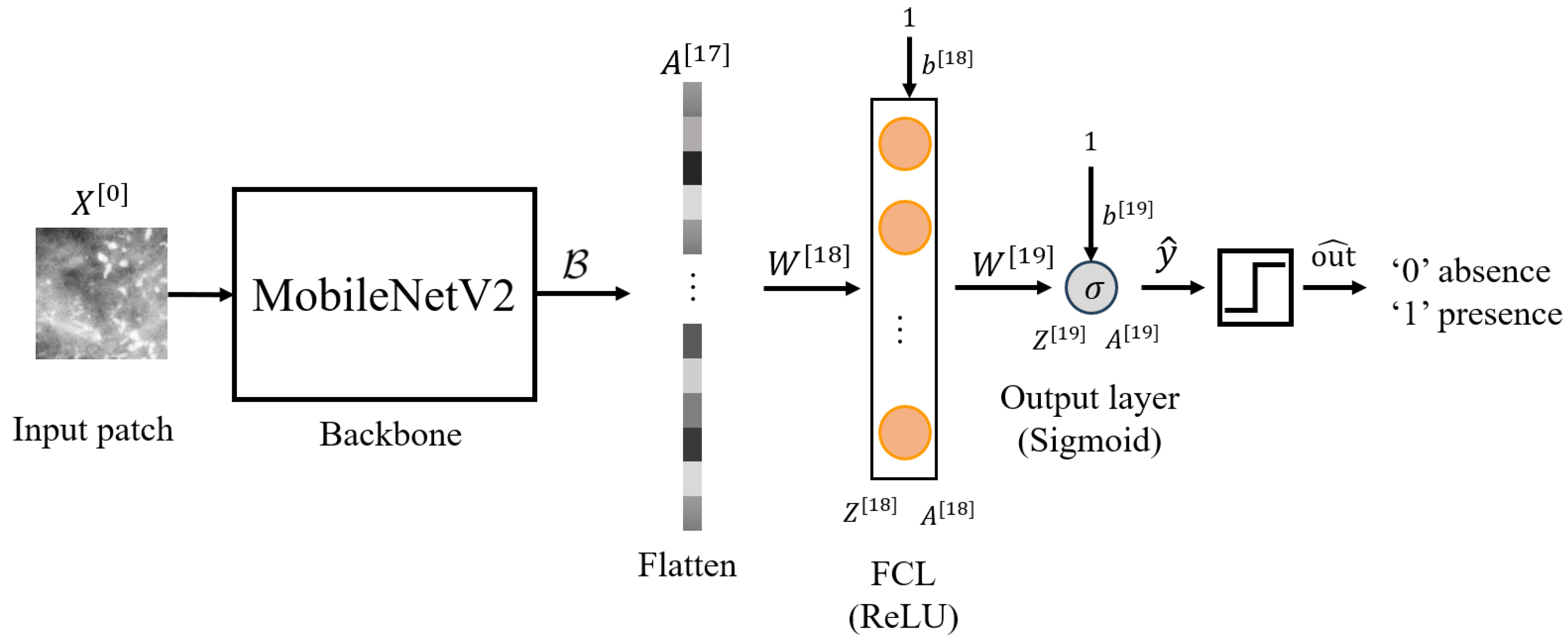
The MobileNetV2 backbone ($\mathcal{B}$) retains the trained weights in [23] with the 70 $\mathsf{\mu }$m resolution. Furthermore, we only trained the weights of the additional layers, namely $W^{\left[18\right]}$ and $W^{\left[19\right]}$. Therefore, the frozen layers can be expressed as

$$\Delta W^{\left[l\right]}=0,\forall W^{\left[l\right]}\in \mathcal{B},\mathrm{where}\Delta W^{\left[l\right]}\mathrm{is}\mathrm{the}\mathrm{weight}\mathrm{update}\mathrm{of}\mathrm{layer}l.$$

The results for Scratch-50, Transfer-50, Scratch-70, Transfer-70, Scratch-100, and Transfer-100 models are shown in

Table 8. Results of models trained from scratch using the MEXBreast datasets and models using TL pretrained on INbreast [23].

Model	Best Epoch	Training Time	Training		Validation		Test
			Acc	Loss	Acc	Loss	Acc	Loss
Scratch-50	95	10 h 38 m	0.9256	9.3884	0.9683	3.3608	0.9607	4.7140
Transfer-50	94	03 h 40 m	0.9739	0.1132	0.9826	0.0743	0.9832	0.0779
Scratch-70	95	15 h 44 m	0.9476	0.1406	0.9928	0.1220	0.9920	3.6220
Transfer-70	76	04 h 12 m	0.9763	0.1251	0.9931	0.1699	0.9927	0.1016
Scratch-100	38	05 h 59 m	0.8560	0.3311	0.8666	0.3309	0.8359	0.3792
Transfer-100	58	02 h 24 m	0.9172	0.2381	0.9218	0.2503	0.8917	0.3030

. Training metrics, including accuracy and loss for training, validation, and test, are summarized. The best validation epoch for each model and the total training time is also shown.

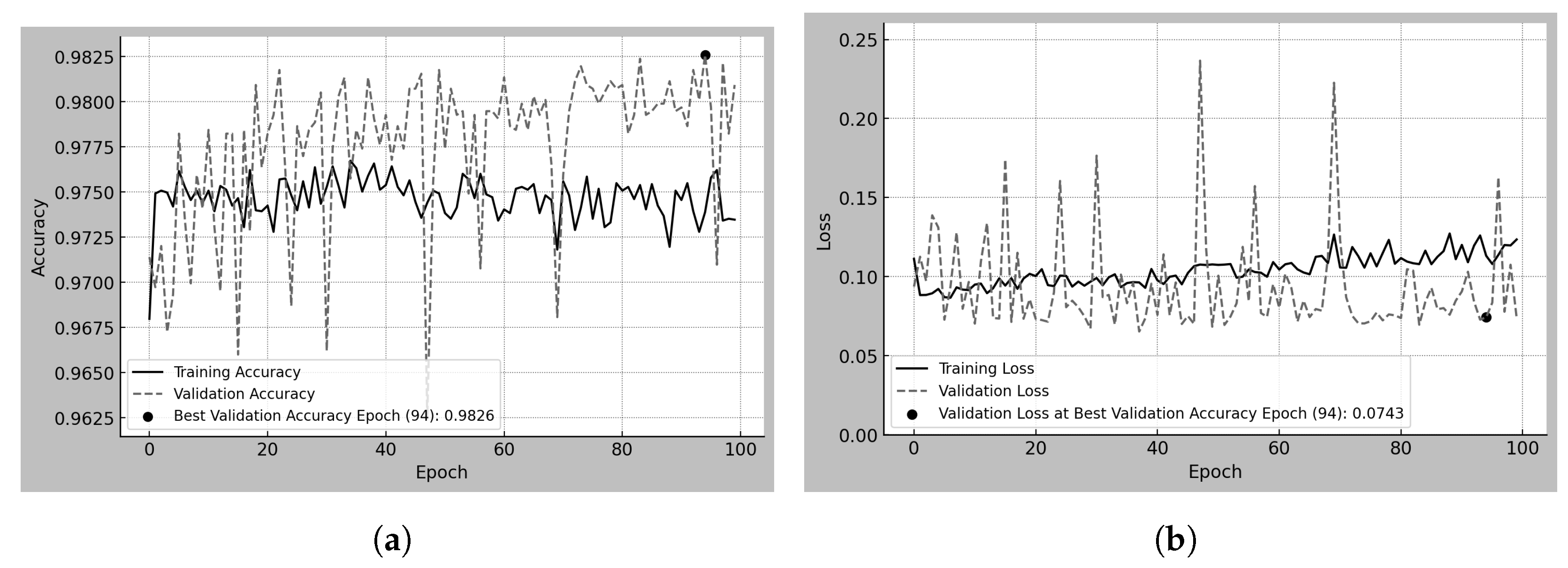
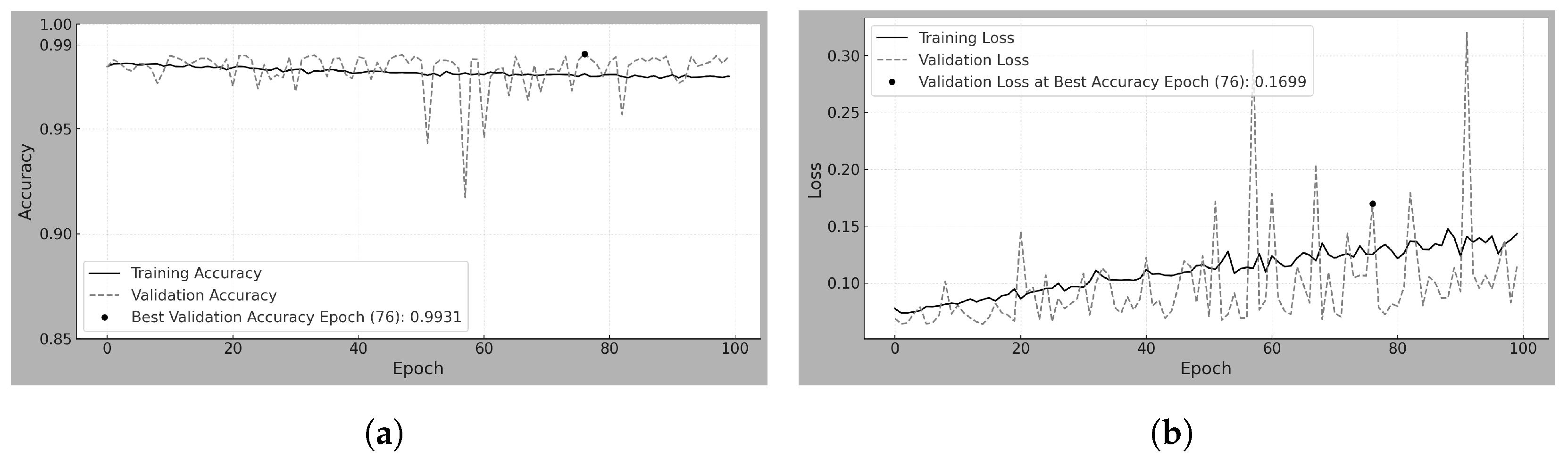
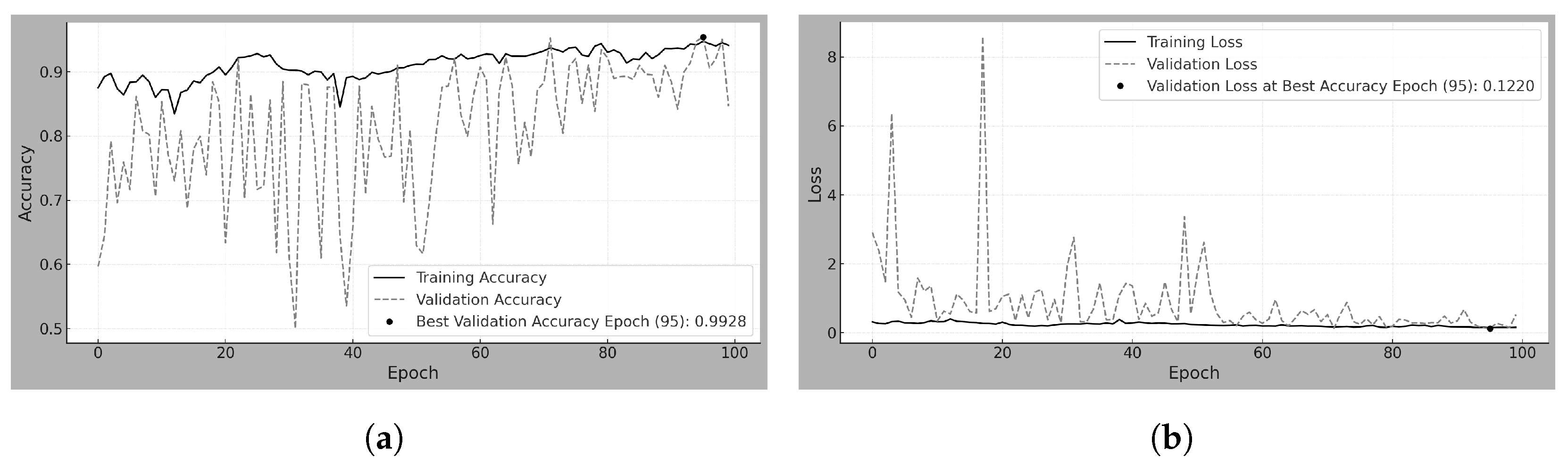
Figure 3a,b present the training and validation accuracy and loss over 100 epochs for the Scratch-50 model, which was trained from scratch using 50 $\mathsf{\mu }$m resolution patches. Figure 4a,b correspond to the Transfer-50 model, which was trained using feature extraction from a pretrained version at 70 $\mathsf{\mu }$m. Similarly, Figure 5a,b and Figure 6a,b depict the same metrics for the Scratch-70 and Transfer-70 models. Finally, Figure 7a,b and Figure 8a,b depict the same metrics for the Scratch-100 and Transfer-100 models. In all cases, the model corresponding to the epoch with the highest validation accuracy was saved and later used for evaluation. Each figure includes a visual marker and a legend indicating the epoch at which this maximum validation accuracy was achieved.

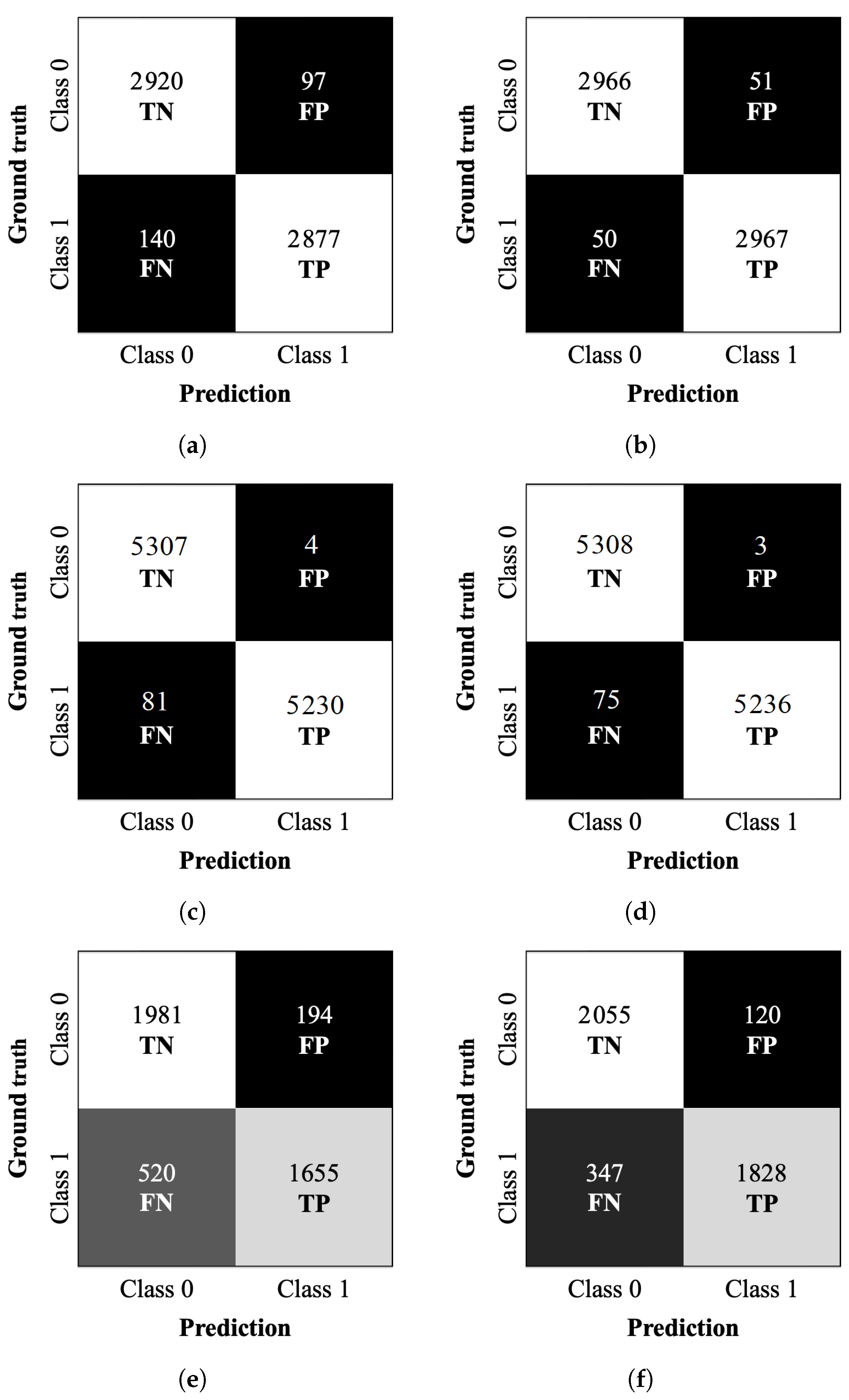
Confusion matrices were calculated for the test datasets corresponding to the Scratch-50, Transfer-50, Scratch-70, Transfer-70, Scratch-100, and Transfer-100 models. The matrices are shown in Figure 9. The matrices summarize the relationships between the predicted and true classes and provide additional insights into the models’ generalization capabilities. The true negatives (TN) are the number of correctly classified negative samples (in our case, the true class 0). The false positives (FP) are the number of negative samples classified as positive (number of true class 0 classified as class 1). The false negatives (FN) are the number of positive samples classified as negative (number of true class 1 classified as class 0). The true positives (TP) are the number of correctly classified positive samples (in our case, the true class 1).

Evaluation metrics such as accuracy, precision, recall (sensitivity), specificity, and F1-score are summarized in

Table 9. Evaluation metrics from the confusion matrices of Figure 9.

Metric	Scratch-50	Transfer-50	Scratch-70	Transfer-70	Scratch-100	Transfer-100
Accuracy	0.9607	0.9832	0.9920	0.9927	0.8359	0.8917
Precision	0.9674	0.9831	0.9992	0.9994	0.8951	0.9384
Recall	0.9536	0.9834	0.9847	0.9859	0.7609	0.8405
Specificity	0.9678	0.9831	0.9992	0.9994	0.9108	0.9448
F1-score	0.9604	0.9833	0.9919	0.9926	0.8226	0.8867

for all the models.

Accuracy measures the overall correctness of the model. Precision represents the proportion of correctly identified positive samples among all predicted positives. Recall reflects the model’s ability to detect positive cases, while specificity quantifies its ability to identify negative cases correctly. The F1-score is the harmonic mean of precision and recall, providing a single metric that balances both aspects and penalizes large discrepancies between them.

Table 10. Accuracy and loss for the Eval-70 model on the INbreast (from our previous work [23]) and MEXBreast test datasets.

Test Dataset	Accuracy	Loss
INbreast	0.99841	0.00844
MEXBreast	0.98456	0.17292

reports the original test results of the Eval-70 model on the INbreast test dataset, obtained in our previous work [23], and included here only as a reference for comparison, along with the new results obtained on the MEXBreast test dataset in the present study. Figure 10 shows the confusion matrix obtained from the predictions on the MEXBreast test dataset; the evaluation metrics presented in

Table 11. Evaluation metrics acquired from the confusion matrix for the Eval-70 model on the MEXBreast test dataset.

Metric	Value
Accuracy	0.9846
Precision	0.9924
Recall	0.9766
Specificity	0.9925
F1-score	0.9844

were calculated based on this matrix.

4. Discussion

In this section, we provide an analysis and interpretation of the results obtained.

4.1. Scratch-50

Scratch-50 refers to the model trained from scratch using 50 $\mathsf{\mu }$m resolution mammograms from the MEXBreast dataset. Table 8 and Figure 3a,b analyze the training and validation behavior over 100 epochs. Regarding accuracy, the training trend shows a steady increase without abrupt changes, reaching 92.56% at the best validation epoch. However, validation accuracy exhibits high variability across epochs, with sudden fluctuations. Despite this, at the best validation epoch (epoch 95 and accuracy of 96.83%), training and validation accuracy exceeded 92%.

The behavior of the loss reflects the fluctuations observed in accuracy. Observe that the loss does not range between 0 and 1 but reaches a maximum value of 350 during training (see Figure 3b). The high loss is largely due to the 50% decision threshold used for classification. Even when the model correctly classifies a sample as class 1, if the predicted probability is close to 0.5, the loss function penalizes it heavily. Furthermore, the high variability in the patch content contributes to this effect, as the model encounters a wide range of mammographic regions with different levels of complexity.

The BCE loss function (Equation (14)) evaluates the classification performance. Its behavior is strongly influenced by the relationship between the predicted probabilities and the ground-truth labels, as it penalizes predictions based on their confidence: high-confidence correct predictions result in very small loss values; low-confidence correct predictions incur a noticeably higher loss despite being classified correctly; and high-confidence incorrect predictions are heavily penalized, leading to large loss values. As a result, even with a high overall classification accuracy, the loss can remain elevated due to low-confidence or incorrect predictions. This effect is reflected in Table 8, where the test accuracy reached 96% (0.96), while the test loss remained high at 4.71.

Table 9 shows the model’s effectiveness in classifying unseen samples, resulting in an accuracy of 96.07%. The model demonstrates high precision (96.74%) and specificity (96.78%), which indicates a low number of FP (97). The recall (sensitivity) of 95.36% tells us that the model correctly identifies most positive cases, with only 140 FN. The F1-score of 96.04% further supports the balance between precision and recall, showing a well-calibrated classification performance.

4.2. Transfer-50

Transfer-50 refers to the model using TL by freezing the backbone ($\mathcal{B}$) of the pretrained 70 $\mathsf{\mu }$m model [23] (trained on INbreast) and training on 50 $\mathsf{\mu }$m patches from the MEXBreast dataset. Table 8 and Figure 4a,b show that, from the first epoch, the accuracy exceeds 95% due to the transfer of knowledge from the 70 $\mathsf{\mu }$m model. Training and validation accuracies remain stable throughout the process. The range between 96.25% and 98.25%, indicates the absence of abrupt fluctuations.

Similarly, the loss remains stable for validation and training. The values ranging between 0.05 and 0.25, confirming the consistency of the model’s learning process. The narrow range in accuracy and loss suggests that TL approach enables rapid adaptation without significant variability. The confusion matrix in Figure 9b, provides further insight into the model’s classification performance on the testing dataset. The strong contrast between the white and black regions indicates a well-defined separation between correctly and incorrectly classified samples. The completely white diagonal, corresponding to correctly classified cases (2966 TN and 2967 TP), suggests high classification performance.

Likewise, the black diagonal, representing misclassified cases, shows 51 FP and 50 FN, reinforcing the low error rate. The clarity in the separation of these regions visually confirms the model’s ability to distinguish between high accuracy classes. The metrics in Table 9 show the model’s high classification effectiveness. The accuracy of 98.32% depicts the strong separation observed in Figure 9b, where correctly classified cases dominate.

Precision, recall, and specificity remain balanced, all within 98.31–98.34%, indicating that the model maintains consistent performance across both classes. The F1-score of 98.33% further confirms this balance, highlighting the agreement between precision and recall.

4.3. Scratch-70

Scratch-70 is the model trained from scratch on 70 $\mathsf{\mu }$m resolution mammograms from the MEXBreast dataset. Table 8 and Figure 5a,b show the training and validation behavior over 100 epochs. Regarding accuracy, the training curve increases steadily without abrupt changes, reaching 99.28% at the epoch with the best validation result. In contrast, the validation accuracy exhibits high variability across epochs, with noticeable fluctuations. Nonetheless, at the best validation epoch (epoch 95), both training and validation accuracy exceeded 92%. Concerning the loss metric, although the overall loss ranges between 0 and 8, as depicted in Figure 5b, it remains close to zero for most of the epochs.

Table 9 shows a test accuracy of 99.20%, consistent with the rest of the evaluation metrics. The only metric showing a slight deviation is recall, with a value of 98.62%, which suggests the presence of a few FN. In practical terms, this means that out of 100 truly positive cases, the model might fail to detect fewer than two.

4.4. Transfer-70

Transfer-70 refers to the model trained using TL by freezing the backbone ($\mathcal{B}$) of a pretrained model [23] (originally trained on 70 $\mathsf{\mu }$m resolution patches from the INbreast dataset) and retraining on 70 $\mathsf{\mu }$m patches from the MEXBreast dataset. Table 8 and Figure 6a,b show that, from the very first epoch, both training and validation accuracies exceeded 97% due to the transfer of knowledge from the pretrained 70 $\mathsf{\mu }$m model. Accuracy values remained stable throughout the training process, without abrupt fluctuations, except for a few noticeable variations in validation accuracy between epochs 55 and 65.

Regarding the loss metric, training loss remained within the 0 to 0.15 range, while validation loss mostly stayed in that same range, with occasional spikes reaching up to 0.30. Nevertheless, the overall variation remained small. Although the trend shows a gradual increase in validation loss over the epochs, the fluctuation remains within a narrow band.

The confusion matrix in Figure 9d clearly shows a strong contrast between correct and incorrect classifications, with only 3 FP among 5308 TN. This visual distinction highlights the model’s reliability in accurately identifying negative cases.

As summarized in Table 9, accuracy, precision, specificity, and F1-score all exceed 99%, with the exception of recall, which reaches 98.59%. This means that, out of every 100 positive cases, more than 98 are correctly identified as TP, with fewer than two misclassified as FN.

4.5. Scratch-100

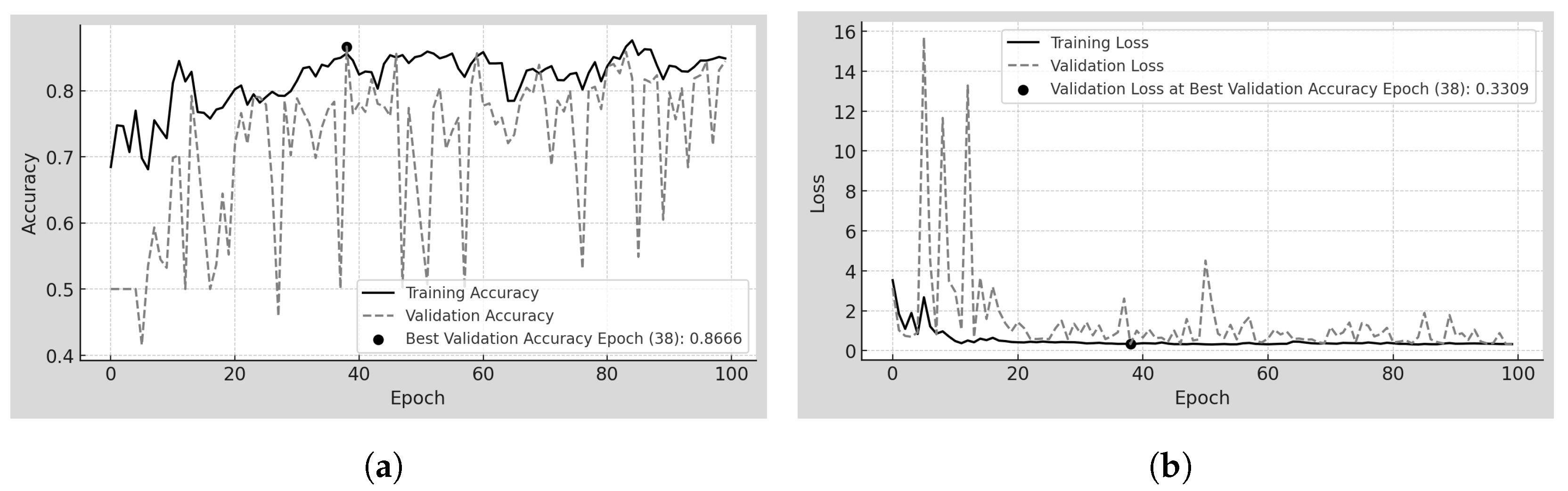
Scratch-100 is the model trained from scratch on 100 $\mathsf{\mu }$m resolution mammograms from the MEXBreast dataset. Table 8 and Figure 7a,b show the training and validation behavior over 100 epochs analyzed. Regarding accuracy, a separation between training and validation accuracy is observed throughout most epochs, though this gap remains relatively small despite being visually noticeable. Training accuracy ranges from just below 0.7 to 0.9, while validation accuracy fluctuates between 0.4 and 0.9. However, both metrics converge at the optimal epoch (epoch 38), with the validation accuracy slightly exceeding the training accuracy, reaching 86.66%.

The limited dataset size, consisting of only 22,130 patches, including augmented samples, may have influenced the early stabilization of the model, as the best epoch occurred at 38 rather than later in training. Regarding loss, both training and validation follow a similar trend. However, between epochs 5 and 15, validation loss exhibits sharp peaks ranging from 1 to 16, suggesting higher variability in performance during this phase.

The confusion matrix of Figure 9e provides further insight into the model’s classification performance on the testing dataset. Unlike previous models, the contrast between the white and black regions is less pronounced, with intermediate gray tones appearing, indicating a higher number of misclassified samples. The model correctly classifies 1981 TN and 1655 TP. However, it also yields 194 FP and 520 FN. The lighter shading in the FN cell suggests a higher number of missed positive cases than previous models, indicating greater difficulty detecting class 1 instances.

The overall pattern in the confusion matrix shows a tendency of the model to misclassify positive samples as negative more frequently than vice versa. This imbalance is influenced by the limited dataset size, as previously noted in the training behavior. The final accuracy and loss values for the Scratch-100 model, presented in Table 8, provide an overview of the model’s classification performance across training, validation, and test datasets. The accuracy remains relatively stable, with values of 85.60% in training, 86.66% in validation, and 83.59% in testing, showing a slight decrease in the latter. The loss values remain close across datasets, with 0.3311 in training, 0.3309 in validation, and 0.3792 in testing. The increase in test loss compared to training and validation suggests performance degradation when evaluating previously unseen data.

Unlike previous models, where the loss function heavily penalizes predictions close to the 50% classification threshold, the less pronounced effect observed in Scratch-100 may be attributed to the limited number of samples, which could influence the overall distribution of predicted probabilities.

4.6. Transfer-100

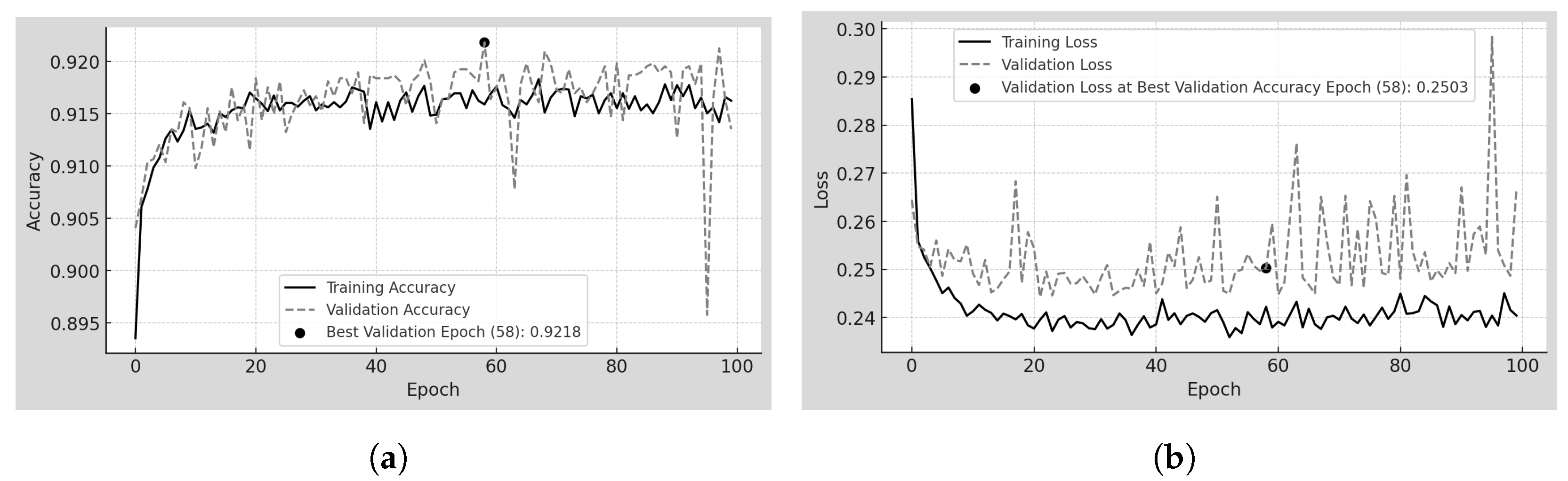
Transfer-100 is the model using TL by freezing the backbone ($\mathcal{B}$) of the pretrained 70 $\mathsf{\mu }$m model [23] (trained on INbreast) and training on 100 $\mathsf{\mu }$m patches from the MEXBreast dataset. In Table 8 and Figure 8a,b the training and validation behavior over 100 epochs is analyzed. Unlike Scratch-100, the accuracy trends in training and validation follow a similar pattern, except for a few prominent peaks, particularly near epoch 100 in validation. However, accuracy remains within a narrow range, from 89.5% to 92.0%, indicating minimal variability. The model achieves its best validation accuracy early in training, reaching 92.18% at epoch 58.

Regarding loss, the trends in training and validation do not fully converge, but the separation between them is minimal. Training loss remains between 0.24 and 0.25, while validation loss fluctuates slightly between 0.25 and 0.26. Additionally, the overall loss values range only from 0.24 to 0.30, confirming the low variability in error throughout training.

The confusion matrix in Figure 9f provides further insight into the model’s classification performance on the testing dataset. The correctly classified cases, 2055 TN and 1828 TP form a diagonal that, although not completely white, appears in a very light gray tone, indicating a high proportion of correctly classified samples.

The misclassified cases, 120 FP and 347 FN, are represented by darker shades, though not entirely black. The FN cell, in particular, appears in a dark gray tone, suggesting that the model still misclassified some positive cases as negative, but at a lower rate compared to other misclassifications scenarios. The overall distribution of values in the confusion matrix reflects a relatively stable classification performance, with a clear distinction between correctly and incorrectly classified samples.

The metrics in Table 9 show the quantitative evaluation of the model’s classification effectiveness. The accuracy of 89.17% indicates that most of the samples were correctly classified. The model achieves a precision of 93.84%, meaning that in most of the cases class 1 is predicted correctly. The specificity of 94.48% further supports this. It indicates a strong ability to identify negative cases correctly (class 0).

The recall (sensitivity) of 84.05% suggests that the model correctly identifies most positive cases, though the presence of 347 FN in the confusion matrix indicates that some positive cases were misclassified as negative. The F1-score of 88.67% reflects a balance between precision and recall, confirming that the model maintains a stable trade-off between these two metrics.

4.7. Eval-70

Eval-70 is the model pretrained on the INbreast dataset at 70 $\mathsf{\mu }$m [23], directly evaluated on the MEXBreast dataset at the same resolution. Table 10 presents the accuracy and loss values for the Eval-70 model when tested on the INbreast and MEXBreast test datasets. Since this model was previously trained on INbreast, its performance on this dataset is a reference for evaluating its generalization to MEXBreast.

On the INbreast test dataset, the model achieves an accuracy of 99.84% with a loss of 0.00844. However, when tested on the MEXBreast test dataset, the accuracy decreases to 98.46%, and the loss increases to 0.17292. While the model still performs well, the increase in loss suggests a higher uncertainty in predictions on MEXBreast compared to INbreast.

The variation in loss values may be related to differences in the size and characteristics of the test datasets. The pretrained model on INbreast was trained using only 10,088 patches (including augmented data), while it was evaluated on 10,622 non-augmented patches from MEXBreast. Notably, the test set is even larger than the original training set. The increased size and diversity of the MEXBreast test set may contribute to the observed variability in prediction confidence.

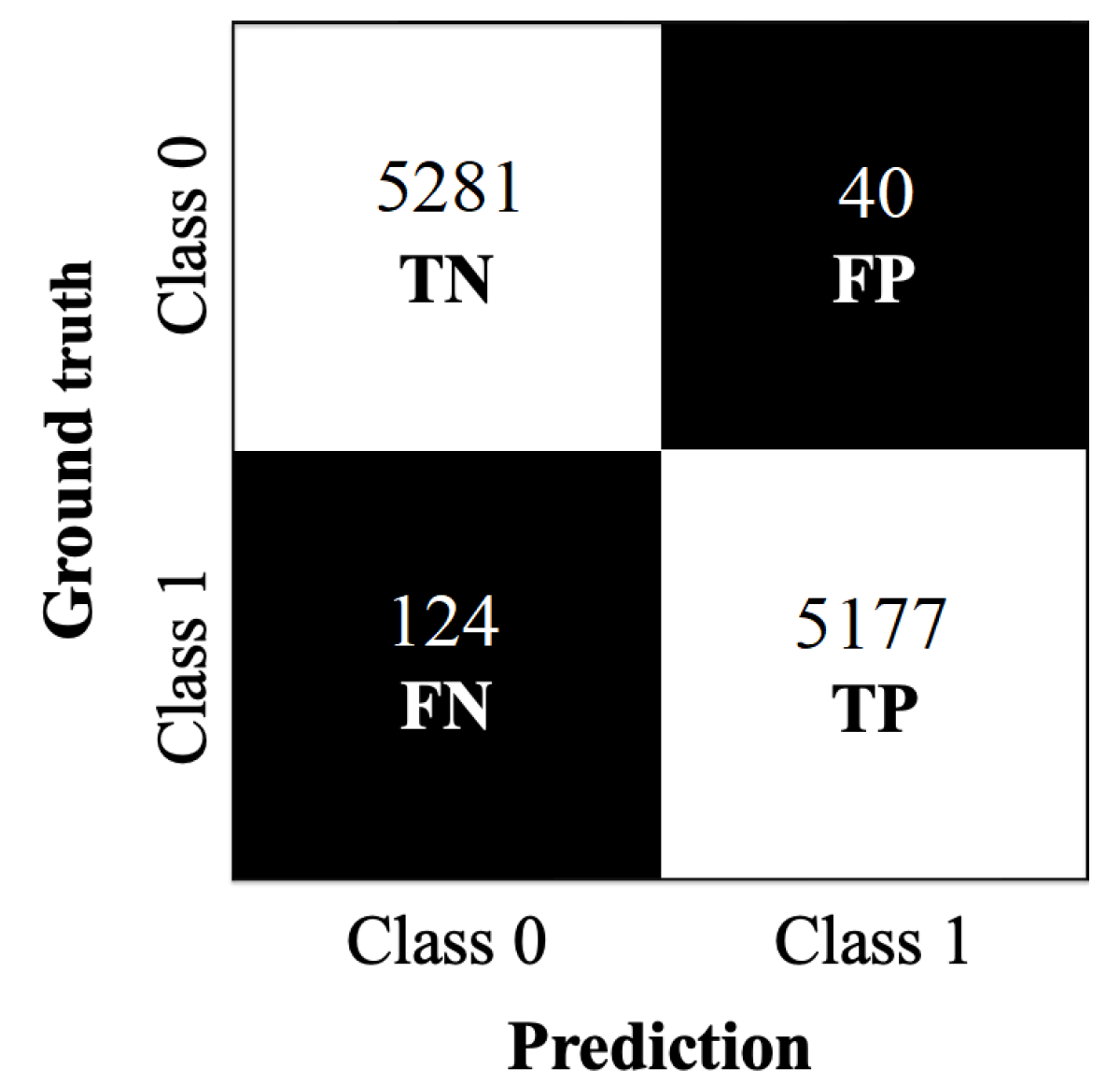
The confusion matrix in Figure 10 provides further insight into the classification performance of the Eval-70 model on the MEXBreast test dataset. The correctly classified cases, 5281 TN and 5177 TP, form an entirely white diagonal, reflecting the large number of correct predictions in both classes.

The misclassified cases, 40 FP and 124 FN, appear in completely black regions, meaning that these errors represent only a small fraction of the total samples. The overall distribution of values in the confusion matrix visually confirms the model’s strong classification performance, with a well-defined separation between correctly and incorrectly classified samples.

The performance metrics in Table 11 show the strong classification performance of the Eval-70 model on the MEXBreast test dataset with an accuracy of 98.46%. The model precision is 99.24%. The specificity of 99.25% shows that the model is highly reliable in identifying negative cases (class 0).

The recall (sensitivity) of 97.66% and the F1-score of 98.44% suggest that the model correctly identifies nearly all positive cases, and consequently, precision and recall are closely aligned.

5. Conclusions and Future Work

In this section, we present the conclusions based on the results obtained, followed by a description of possible directions for future work.

5.1. Conclusions

In this paper, we proposed a cross-domain TL architecture for detecting MCCs in mammographic patches at 50 $\mathsf{\mu }$m, 70 $\mathsf{\mu }$m, and 100 $\mathsf{\mu }$m resolutions from the multiresolution MEXBreast database [33,34]. The input consists of 1 cm² patches systematically extracted from mammograms, enabling resolution-consistent handling across datasets of different resolutions. The architecture comprises a MobileNetV2 backbone to extract a multidimensional output feature map $\mathcal{B}$, followed by a flattening layer to produce a one-dimensional vector, an FCL with 2048 ReLU units, and a final output layer with a single-unit FCL for binary classification.

Three models were trained from scratch, Scratch-50, Scratch-70, and the Scratch-100, using patches of mammograms at 50 $\mathsf{\mu }$m, 70 $\mathsf{\mu }$m and 100 $\mathsf{\mu }$m resolution. The resulting accuracies were 96.07%, 99.20%, and 83.59%, respectively. Afterward, a model pretrained on patches at 70 $\mathsf{\mu }$m resolution from the INbreast database [23] was subsequently adapted to 50 $\mathsf{\mu }$m, 70 $\mathsf{\mu }$m and 100 $\mathsf{\mu }$m resolutions through TL, resulting in the Transfer-50, Transfer-70 and Transfer-100 models. Transfer-50 model achieved an accuracy of 98.32%, Transfer-70 model achieved 99.27% and the Transfer-100 model achieved 89.17%, outperforming their corresponding model trained from scratch. Furthermore, the time reduction using TL was 65.5% for 50 $\mathsf{\mu }$m, 73.3% for 70 $\mathsf{\mu }$m and 59.9% for 100 $\mathsf{\mu }$m.

The pretrained model on 70 $\mathsf{\mu }$m patches, referred to as Eval-70, was tested on the MEXBreast test dataset for 70 $\mathsf{\mu }$m, achieving an accuracy of 98.46%. The results showed that the proposed CNN with TL consistently improved classification accuracy and reduced training time compared to models trained from scratch. Furthermore, the model demonstrated the ability to detect MCCs across different resolutions while maintaining high classification performance. Nevertheless, achieving reliable models depends on the availability of well-annotated datasets, which are essential for ensuring accurate training and evaluation in medical imaging.

Three different models were evaluated for the same spatial resolution of 70 $\mathsf{\mu }$m: Scratch-70, Transfer-70, and Eval-70. Among them, Transfer-70 achieved the best performance, followed by Scratch-70 and then Eval-70. This outcome indicates that even when models operate within the same spatial domain, such as 70 $\mathsf{\mu }$m, it does not necessarily imply that all will perform equally well. Although performance levels may be similar, the optimal approach is to leverage the knowledge acquired by one model and transfer it to another, even within the same spatial domain. This strategy remains valid when the spatial domain changes as well.

5.2. Future Work

Future work could explore the evaluation of trained models using synthetic mammographic patches, introducing controlled variations in the distribution, size, shape, orientation, and location of MCCs within breast tissue. The evaluation could be conducted through a web-based application featuring configurable controls to define the desired characteristics of the generated patches. The controlled generation of synthetic patches would make it possible to include other BI-RADS-defined distribution patterns, beyond the grouped type addressed in the present work, including diffuse, regional, linear, and segmental distributions [11].