Abstract
This paper presents a hybrid indoor localization framework combining time difference of arrival (TDoA) measurements with a swarm intelligence optimization technique. To address the nonlinear optimization challenges in three-dimensional (3D) indoor localization via TDoA measurements, we systematically evaluate the artificial bee colony (ABC) algorithm and chimpanzee optimization algorithm (ChOA). Through comprehensive Monte Carlo simulations in a cubic 3D environment with eight beacons, our comparative analysis reveals that the ChOA achieves superior localization accuracy while maintaining computational efficiency. Building upon the ChOA framework, we introduce a multi-beacon fusion strategy incorporating a local outlier factor-based linear weighting mechanism to enhance robustness against measurement noise and improve localization accuracy. This approach integrates spatial density estimation with geometrically consistent weighting of distributed beacons, effectively filtering measurement outliers through adaptive sensor fusion. The experimental results show that the proposed algorithm exhibits excellent convergence performance under the condition of a low population size. Its anti-interference capability against Gaussian white noise is significantly improved compared with the baseline algorithms, and its anti-interference performance against multipath noise is consistent with that of the baseline algorithms. However, in terms of dealing with UWB device failures, the performance of the algorithm is slightly inferior. Meanwhile, the algorithm has relatively good time-lag performance and target-tracking performance. The study provides theoretical insights and practical guidelines for deploying reliable localization systems in complex indoor environments.
Keywords:
indoor localization; time difference of arrival; swarm intelligence optimization; multi-beacon fusion; local outlier factor MSC:
94-08
1. Introduction
The proliferation of intelligent terminal devices and the accelerated advancement of IoT technologies have established indoor localization as a fundamental enabling technology for smart cities, industrial automation, and emergency response systems. Conventional global navigation satellite systems exhibit severe localization accuracy degradation indoors due to structural obstructions and multipath effects, rendering them inadequate for practical applications [1,2]. Traditional localization methods face operational limitations or frequent impracticality in industrial settings, particularly with low-power signaling devices and obstructed transmission paths [1]. Despite the high outdoor localization accuracy offered by existing satellite systems [3], emerging cross-domain applications demand more resilient indoor alternatives. In recent years, scholars have increasingly explored multi-sensor fusion strategies to enhance localization robustness and localization accuracy [4,5], combining UWB with inertial navigation systems [6], cameras [7], or WiFi. However, the integration of multiple sensors introduces challenges in hardware cost, power consumption, and system complexity, which hinder scalability for large-scale industrial deployments. Therefore, achieving high-precision and high-reliability indoor localization constitutes a critical research priority.
Currently, the commonly used indoor localization technologies are primarily based on the following: Bluetooth indoor localization [8], infrared indoor localization [9], ultrasonic indoor localization [10], WiFi indoor localization [11], radio-frequency identification (RFID) indoor localization [12], ZigBee indoor localization [13], and ultra-wideband (UWB) indoor localization [14,15], among others. Among these, UWB stands out as a technology with exceptional precision, robustness, and penetration capabilities [16]. Defined by the Federal Communications Commission as a radio-frequency signal occupying a frequency spectrum exceeding 20% of the center carrier frequency or a bandwidth greater than 500 MHz, UWB spreads information across a wide spectrum, enabling high data throughput with minimal energy consumption [17]. Its large bandwidth further provides unparalleled advantages over alternatives like Bluetooth, Zigbee, and RFID, including enhanced ranging accuracy, superior multipath resolution [18], and robustness to interference, making it a leading choice for precision-critical indoor applications.
To achieve high-precision indoor localization, this study adopts UWB technology as the core localization device. In our localization method, based on the time difference of arrival (TDoA) principle, we apply the chimpanzee optimization algorithm (ChOA), a swarm optimization algorithm, to establish the baseline. Building upon this baseline, we propose a multi-beacon fusion localization algorithm incorporating local outlier factor (LOF) weighting. Simulation results demonstrate that the proposed algorithm enables real-time, high-precision tracking of user motion trajectories while exhibiting strong robustness in complex indoor environments, which provides a novel technical approach to addressing challenges such as localization accuracy and noise sensitivity in indoor localization scenarios.
2. Process of the TDoA Algorithm
The TDoA algorithm is a localization technology that relies on the time differences of signals arriving at different receivers. Its fundamental principle involves measuring the time differences of a signal reaching multiple receivers from a target source, then using these differences to calculate the localization of the target [19]. The implementation process is described as follows: when a target emits a signal, receivers at various positions record the arrival times of the signal. Due to the varying distances between the receivers and the target, the arrival times of the signal will differ. By calculating these time differences and considering the propagation speed of the signal (typically, the speed of light), the distance differences between the target and each receiver can be determined [20].
Before the principal analysis, we first define the Euclidean norm symbol () used in our paper:
where v denotes the coordinate dimension of point A and point Z and and denote the coordinate values of the u-th dimension of A and Z, respectively.
In a 2D plane (X-axis and Y-axis), the TDoA localization algorithm estimates the localization of the target by measuring the time differences of signals arriving at different beacons. Assume there are three beacons: beacon 1, serving as the reference beacon, with beacon 2 and beacon 3 functioning as localization beacons. Let the coordinates of the target be ; the coordinates of beacon 1, beacon 2, and beacon 3 be , , and , respectively; and the signal arrival times at each beacon be , , and . The signal propagation speed is denoted by c (typically the speed of light). Using beacon 1 as the reference, the following two time difference equations can be derived [21]:
where the time differences of arrival (TDoA) are defined as follows. The term represents the time difference between the signal arrival at beacon 2 and beacon 1, calculated by the difference of Euclidean distances from the receiver to both stations divided by the speed of light (c). Similarly, denotes the time difference between beacon 3 and beacon 1.
Each TDoA measurement associated with a pair of beacons induces a hyperbolic locus, as shown in Figure 1, as these equations represent two hyperbolas, with beacon 1 as the common reference. A hyperbola is defined as the set of all points in a plane where the difference of the distances to two fixed points (the foci) is constant. Here, the foci correspond to the reference beacon (beacon 1) and another beacon (beacon 2 or beacon 3), with the constant difference determined by the time difference of arrival multiplied by the signal propagation speed (c). The source position is then estimated by finding the intersection of these hyperbolic curves [22].
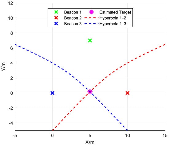
Figure 1.
TDoA hyperbolic localization schematic diagram.
By solving the following system of equations, the localization of the target can be determined:
In a 2D plane, the two hyperbolas typically intersect at two points. However, by considering practical constraints (e.g., signal propagation range), one of the solutions can be eliminated, yielding a unique target coordinate. Through this process, the TDoA algorithm achieves precise target localization in a two-dimensional plane. However, when extending the localization problem to a 3D space, the geometric characteristics of the algorithm change significantly due to the introduction of a new dimensional variable (the Z-axis).
In the case of 3D space, the representation for the TDoA equations will be hyperboloids rather than hyperbolas. A hyperboloid is a surface defined as the set of points where the difference of distances to two fixed points (foci) remains constant. Taking beacon 1 as an example, the 3D TDoA equations can be expressed as
where Q is extended to the target coordinates in 3D space.
In 3D space, the intersection of two hyperboloids forms a spatial curve rather than discrete points. While this curve represents solutions to the 3D TDoA equations, the continuous nature of the intersection makes it impossible to determine a unique target position using a single set of TDoA equations. Therefore, localization with only three beacons in 3D space remains theoretically unachievable. To achieve unique localization in 3D TDoA systems, the introduction of a fourth beacon becomes essential. This configuration generates three independent TDoA equations that intersect at a unique spatial point [16,23]. The mathematical formulation extends as follows:
where the fourth beacon provides the third independent hyperboloid equation () and the intersection of reduces from a spatial curve to discrete points.
Geometric Interpretation:
where denotes the hyperboloid defined by the TDoA constraint between and . This geometric configuration requires three independent hyperboloids (derived from four beacons) to collapse the solution space from a spatial curve to a discrete point. This configuration satisfies the necessary and sufficient condition for the unique 3D localization.
3. Process of the Chimpanzee Optimization Algorithm
We achieve 3D localization using the chimpanzee optimization algorithm (ChOA), a bio-inspired optimization technique that mimics the social behavior and hunting strategies of chimpanzees to solve complex optimization problems [24]. The algorithm operates through two primary phases—the attack expulsion phase and the chasing and encircling phase—iteratively enhancing a population of candidate solutions. In the chasing and encircling phase, candidate solutions (representing chimpanzee individuals) collaboratively explore the search space to surround and track optimal regions. During the attack expulsion phase, dominant solutions aggressively refine their positions while expelling weaker candidates to avoid local optima. The algorithm performs well in a multi-dimensional search space, especially in dealing with complex three-dimensional space localization problems.
The algorithm begins by initializing a population of N individuals, where each individual represents a potential solution in the search space. The position of the q-th individual in the t-th iteration is denoted as , and the search-space boundaries are defined by the minimum and maximum coordinates of the beacons as follows:
where , with M representing the number of beacons, including redundant beacons introduced by the algorithm. Each individual is initialized randomly within these boundaries:
where is a random vector and ⊙ denotes element-wise multiplication.
The fitness of each individual is evaluated using an objective function (), which quantifies the quality of the solution. For beacon localization, the objective function is defined as follows:
where denotes the position of the v-th localization beacon, is the reference beacon, and is the measured distance difference. A lower fitness value indicates a better solution.
In the attack expulsion phase, each chimpanzee randomly attacks or expel other chimpanzees in each iteration to update the location of the attacker or expelled person:
where denotes the updated individual location, denotes the individual location before the update, denotes the p-th individual selected in the t-th iteration at random, denotes random values with a uniform distribution from 0 to 2, t denotes the current number of iterations, and T denotes the maximum number of iterations. If is smaller than , use instead of ; otherwise, the current iteration will be invalidated.
The new solution is then constrained to the search-space boundaries by clamping each coordinate to the predefined minimum and maximum values using element-wise operations:
After each iteration, the global best is updated if a better solution is found:
where denotes the global optimal solution obtained in the t-th iteration, that is, the corresponding to the smallest value of .
In the chasing and encircling phase, chimpanzees move to the global optimal solution to simulate the behavior of surrounding prey:
where the calculation method of G is the same as Equation (12).
The algorithm terminates if the fitness improvement falls below a threshold () for a specified number of iterations ():
When the iteration is stopped, is obtained as the localization coordinates estimated by the ChOA. In the following steps, the localization coordinates are used as the preliminary localization coordinates of the proposed algorithm.
4. LOF Weighted Fusion Mechanism
Traditional TDoA localization algorithms are constrained by hardware precision limitations and environmental interference, often resulting in localization accuracy that fails to meet high-precision requirements. Due to random disturbances such as multipath effects, clock synchronization errors, and environmental noise during signal propagation, the coordinates output by the algorithm typically exhibit a normal distribution, with higher point density near the true localization. Additionally, real-world application scenarios often involve a large number of redundant beacons. Leveraging these characteristics, this study selects a group of beacons (including redundant ones) covering the target area and generates a set of candidate coordinates using each beacon as a reference node. The LOF algorithm [25] is then applied to quantify the outlier degree of each coordinate point. Finally, a linear weighted average of all candidate coordinates is calculated based on their LOF values, where points closer to the main distribution (lower outlier degrees) are assigned higher weights, thereby obtaining the final estimated position.
Now, let us provide the weighted multi-beacon fusion process with the LOF strategy. For each point (p), compute the Euclidean distance to all other points (o) in the dataset.
where and denote the estimated coordinates obtained from the combination of the -th and -th beacons(), respectively, and denotes the Euclidean distance between and .
For the convenience of further explanation, we define the set of k points closest to as and the distance from point to its k-th nearest point as . Then, we can define the reachability distance from point to point as follows:
where is the reachability distance from point to point .
Then, compute the local reachability density (LRD) for point as the inverse of the average reachability distance to its k nearest neighbors:
where denotes the LRD for point .
Calculate the LOF score for point as the ratio of the average LRD of its k nearest neighbors to its own LRD:
where denotes the LOF score of point and denotes the average local reachability density of the neighbors of point .
Next, we use LOF values to weight multiple preliminary estimated coordinates. The weight () of each point () can be calculated by the following formula:
where denotes the weight corresponding to point and denotes a small constant to prevent division by zero.
where denotes the 3D coordinate of the final localization point () of the algorithm and denotes the 3D coordinate of the preliminary estimated localization point () of the combination of with the tenth beacon.
According to the algorithm proposed in our paper, the final estimated coordinate point (), which is fused by multiple localization coordinate points preliminarily estimated by the group optimization algorithm through LOF, is the final output of the algorithm.
The proposed 3D localization approach is shown in Algorithm 1, which is explained as follows in detail.
- Step 1:
- We set up M TDoA equations with M sets of beacons as reference beacons and calculate the fitness equation () of each beacon.
- Step 2:
- The search range of the ChOA is determined according to the beacon coordinates (E), and ChOA iteration is performed in the search range. When there is still no improvement after several iterations, the current best chimpanzee individual coordinate is output.
- Step 3:
- Calculate the LOF value of each preliminary localization coordinate to obtain the weight corresponding to each preliminary localization coordinate and fuse the preliminary localization coordinates according to the weight to obtain the final localization coordinate ().
Intuitively, the proposed localization approach begins by calculating TDoA measurements from N neighboring beacons (including redundant ones) around the target beacon. These N beacons are systematically divided into N distinct combinations, each employing a different reference station. For each combination, a corresponding TDoA equation system is constructed and solved through the ChOA, generating N initial coordinate estimates. The LOF algorithm then evaluates spatial consistency by calculating outlier scores for these solutions. The final position is determined through linear weighted summation, where weights are inversely proportional to the computed outlier scores. This redundant beacon configuration ( for 3D localization) enhances system robustness against signal anomalies while maintaining computational efficiency.
| Algorithm 1 The proposed localization approach | |
| Input: | ▹ beacon coordinates |
| ▹ TDoA measurements (s) | |
| ▹ Signal propagation speed | |
| ▹ ChOA parameters | |
| ▹ LOF parameter | |
| Output: | ▹ Final position |
Step 1: Execute the Baseline Algorithm
| |
5. Numerical Simulations
We use MATLAB R2022b for the subsequent simulation experiments.
In the 3D simulation environment, we systematically evaluate multiple swarm optimization algorithms by quantifying their localization errors and computational costs. A comparative analysis is subsequently conducted to quantify the improvements in localization accuracy and robustness of the proposed algorithm against baseline methods.
A 3D localization environment is shown in Figure 2, where a total of eight beacons are set up, positioned at each of the eight corners of the cubic localization area. In the simulation experiment, we set the coordinates of the eight beacons as , , , , , , , and . The coordinates of the localization point are set as .
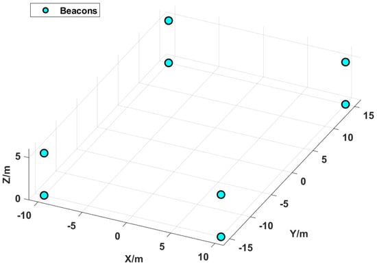
Figure 2.
Beacon localization distribution map.
5.1. Compared Swarm Optimization Algorithms and Data Processing
In the selection phase of swarm optimization algorithms, our study compared the performance of the bat algorithm (BA) [26], gray wolf optimizer (GWO) [27], artificial bee colony (ABC) algorithm [28], and chimpanzee optimization algorithm (ChOA) [24]. The relevant simulation data are presented as follows.
In subsequent experiments, we fix some operational parameters of the algorithms based on experience, among which the pulse frequency range of the Bat Algorithm (BA) is set from 0 to 2 (indicating that the frequency is randomly generated between 0 and 2), the loudness is set to (representing moderate search intensity), the pulse rate is set to (indicating a 50% probability of conducting global search), and the scout-bee trigger threshold of the Artificial Bee Colony (ABC) algorithm is set to 15 (meaning that if there is no improvement for 15 consecutive times, the position of that bee will be reset). For the Gray Wolf Optimizer (GWO) and chimp optimization algorithm (ChOA), only the population parameters shared by all algorithms, the convergence threshold, and the maximum number of non-improving iterations allowed by the algorithm () can be set. The population parameters of all algorithms are discussed in subsequent simulation experiments. Since the population parameter (N), the convergence threshold (), and the maximum number of non-improving iterations () interact with each other, we choose to fix two secondary parameters to simplify the experimental results. The convergence threshold and are defined for the adaptive convergence of the algorithm; once the algorithm converges to a sufficiently small value, there is no need to consume computing resources for further iterative improvement. Therefore, based on experience, in subsequent experiments, the convergence threshold of the algorithm is set to , and the maximum number of non-improving iterations is set to 30.
In each of the subsequent sets of simulation experiments, a random point in 3D space is selected as the coordinate to be estimated by the algorithms, and the performance of various algorithms under different conditions is studied. This study employs the Monte Carlo simulation method, acquiring data samples through 2000 independent repeated simulations. To ensure the robustness of the simulation results, the trimmed mean method is applied for data processing, with the specific approach described as follows: the simulation data are arranged in ascending order based on their values, after which the top % and bottom % of extreme values are removed, and the arithmetic mean of the remaining 95% of data is calculated as the final result. This data processing method effectively reduces the impact of outliers on the simulation results while preserving the central tendency of the primary dataset, thereby enhancing the reliability of the data and ensuring that the analysis remains grounded in the inherent distribution characteristics of the majority of measurement samples.
To more intuitively illustrate the subsequent experimental process of our paper, we created the experimental flowchart shown in Figure 3 for reference.
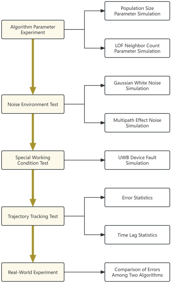
Figure 3.
Experimental flowchart.
5.2. Analysis of Population Size Impact
To investigate the impact of optimization algorithm parameters on algorithm performance, we design a localization accuracy experiment based on different population sizes, with the LOF neighbor count parameter (k) set to 3 in this simulation. As shown in Figure 4, for the four optimization algorithms and the proposed algorithm, we conducted localization accuracy tests with various population sizes ranging from 5 to 160, with a step size of 5, and added Gaussian white noise with a standard deviation of m to the simulation. According to the experimental results, we found that among the four optimization algorithms, ChOA has the fastest convergence speed and the highest localization accuracy after convergence. Moreover, the proposed algorithm further improves the convergence speed with respect to population size and the localization accuracy after convergence on the basis of ChOA. In subsequent experiments, unless otherwise specified, the population size of the algorithms is fixed at 150.
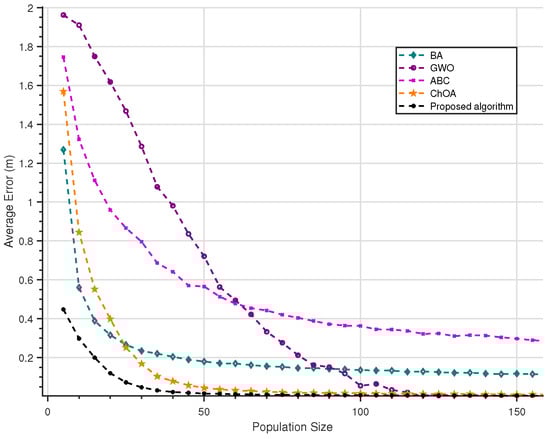
Figure 4.
Population size error curve graph.
5.3. Analysis of LOF Neighbor Count Impact
To investigate the impact of the LOF neighbor count on the accuracy of the localization algorithm, we design a simulation experiment targeting the LOF neighbor count parameter (k). In the experiment, the LOF neighbor count parameter (k) was set to range from 2 to 7 with a step size of 1. The experimental results, as shown in Figure 5, indicate that the algorithm achieves the highest accuracy when the LOF neighbor count parameter (k) is set to 3. Therefore, the LOF neighbor count parameter is fixed at 3 in all subsequent experiments.
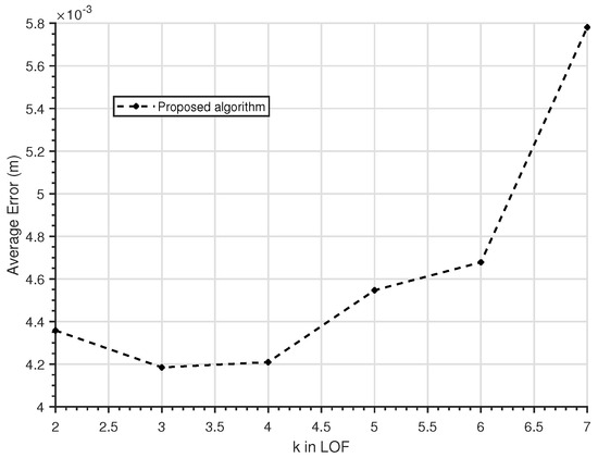
Figure 5.
LOF neighbor count parameter curve graph.
5.4. Gaussian White Noise Test
We conducted a simulation experiment involving Gaussian white noise on four optimization algorithms and the proposed algorithm. In these experiments, we tested the localization errors of different algorithms under 11 noise environments with standard deviations ranging from 0 m to m (with a step size of 0.05 m) to verify the localization performance of our algorithm in a Gaussian white noise environment. According to an in-depth analysis of the simulation results presented in Figure 6, the localization accuracy of the ChOA is significantly superior to that of the other three optimization algorithms under different error standard deviations, indicating that the localization algorithm employing the ChOA possesses favorable precision and robustness. The simulation results confirm that the ChOA not only achieves outstanding localization accuracy in typical operational scenarios but also maintains strong robustness under various error conditions, making it particularly suitable for practical applications with low to moderate standard deviations in localization error values. Meanwhile, we can also observe that the proposed algorithm further improves the localization accuracy in each noise segment on the basis of the ChOA. As shown in the figure, under various noise intensity conditions, the localization error curve of the improved algorithm proposed in this paper always lies below that of the ChOA, and it exhibits a more gradual growth trend, especially within the range of localization errors with medium and high standard deviations. The simulation data confirm that the improved algorithm is superior to the original ChOA in terms of both localization accuracy and robustness.
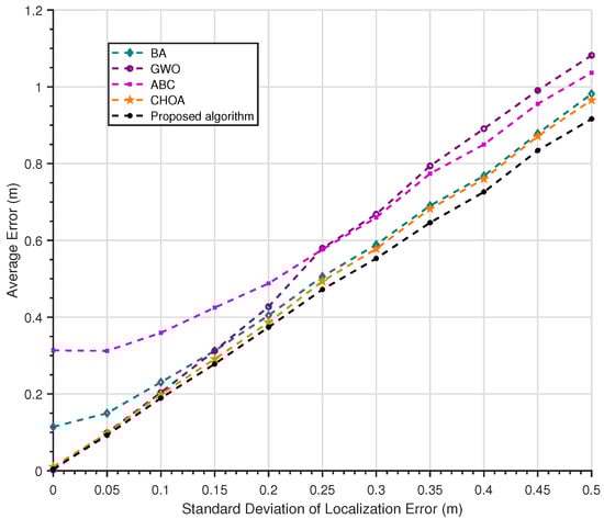
Figure 6.
Gaussian white noise error curve graph.
5.5. Multipath Effect Test
To verify the localization accuracy and robustness of the algorithm in a noise environment with multipath effects, we designed a simulation experiment for such an environment. In the experiment, we fixed the standard deviation of Gaussian white noise at m and added multipath effect noise with an occurrence probability ranging from 0 to (with a step size of ). The multipath effect generates random additional distance measurements in the range of m to m. As shown in Figure 7, with the increase in the occurrence probability of multipath effects, all types of algorithms maintain a similar fluctuation trend in localization accuracy. Moreover, the localization curves of our algorithm and the ChOA (used as the baseline algorithm) show a high degree of consistency in the multipath noise environment. This indicates that the advantages of our algorithm in noise environments are more evident in Gaussian white noise environments, while its anti-interference performance against multipath effects is comparable to that of the ChOA, which serves as the baseline.
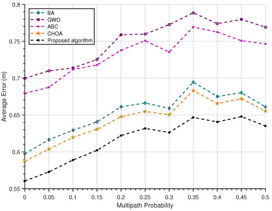
Figure 7.
Multipath effect error curve graph.
5.6. UWB Device Fault Test
We also conducted simulation tests on UWB device faults. Since the probability of UWB device faults in real-world scenarios is extremely low, we significantly increased the probability of UWB device faults in the simulation to highlight the impact of sensor faults on the algorithm’s localization results. As shown in Figure 8, we added a UWB device fault probability ranging from 0 to 0.05 (with a step size of 0.005) to a simulation environment without other interferences and plotted the localization accuracy of different algorithms under 11 such probabilities. When a UWB device fault occurs, an error ranging from 2 m to 5 m arises. From the localization results, it is easy to observe that among the four optimization algorithms, the ChOA has the best adaptability to UWB device faults. However, the proposed algorithm exhibits slightly poorer adaptability to UWB device faults than the ChOA, so it is more sensitive to device quality than the ChOA.
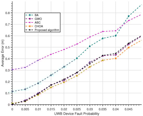
Figure 8.
UWB device fault error curve graph.
5.7. Circular Motion Trajectory Tracking Test
Our study conducted a simulation to validate the localization performance of the proposed algorithm. The simulation scenario is designed as follows: a circular motion trajectory with a radius of m is constructed, centered at the point expressed as in the space where the localization beacon is located. Along this circular trajectory, 150 sampling points are uniformly selected for testing. During the simulation, the standard deviation of localization error is set to m, the occurrence probability of multipath effects is set to , and the proposed algorithm is applied to perform localization calculations at each sampling point.
As shown in Figure 9, the simulation results demonstrate that the localization trajectory generated by the algorithm closely follows the target motion trajectory, exhibiting only minor fluctuations within a small range, which indicates excellent target tracking performance.
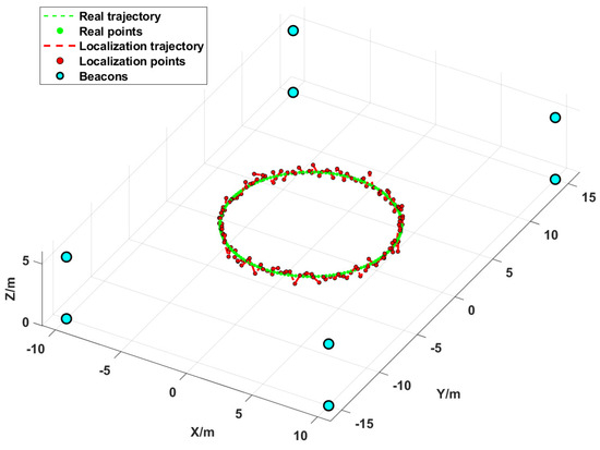
Figure 9.
Circumferential trajectory diagram.
We record the localization error of each sampling point on the trajectory for this experiment. As shown in Figure 10, the localization error of each point fluctuates between 0 and 1 m, and the localization error values are mainly concentrated around the mean value of m, showing a relatively concentrated error accuracy performance.
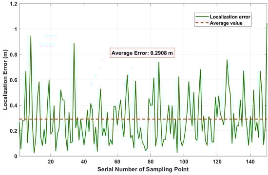
Figure 10.
Trajectory localization error curve graph.
We also record the time lag of each sampling point, which represents the algorithm’s execution time and can characterize the algorithm’s time complexity. As shown in Figure 11, the time lag is relatively high at the beginning of the algorithm’s execution, possibly due to the simulation software’s CPU invocation logic. During subsequent execution, the time lag decreases and fluctuates around the mean value. The algorithm’s time lag is mainly concentrated between and s, which can meet the requirements of most localization scenarios.
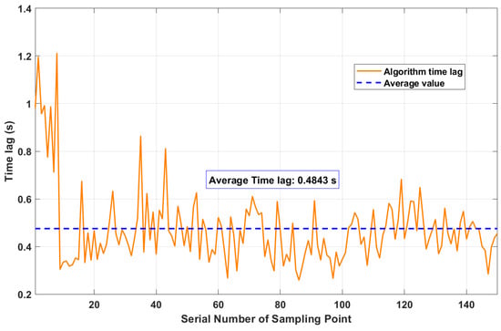
Figure 11.
Trajectory localization time-lag curve graph.
Since the number of beacons can affect the time lag of the proposed algorithm, although there are countless combinations of the number and placement positions of beacons, making it difficult to comprehensively study through experiments, we hereby explain it from a theoretical perspective. Suppose the time complexity of the LOF algorithm is , the time complexity of the the ChOA is , and the number of beacons is U; then, the time complexity of the proposed algorithm is . Therefore, the time complexity of the proposed algorithm has a linear relationship with the sum of the time complexities of the LOF algorithm and the ChOA. Since the number of beacons determines the number of points that need to be calculated by the LOF algorithm and the cube of the number of such points is proportional to the time complexity of the LOF algorithm, the greater the number of beacons, the higher the computational cost of the LOF algorithm. However, the number of beacons used in this paper is not large, and the computational cost of the LOF algorithm is reflected in the algorithm’s time-lag diagram, which is within an acceptable range.
6. Real-World Experiment
We conducted an algorithm accuracy test experiment in a real-world environment and set up a localization scenario, as shown in Figure 12. In the scenario, the positions of the UWB anchors placed on the black brackets at the four corners are , , , and , while the positions of the UWB anchors placed under the black brackets at the four corners are , , , and . The localization tag is placed on the black bracket in the center of the scenario, with its coordinates being . A total of 500 sets of data were recorded in this experiment. Due to the existence of scenario layout errors in the real scene and variations in the actual measurement and estimation of the true coordinate position of the localization tag, its true coordinates may not be truly accurate. Meanwhile, UWB devices have their own volumes, leading to deviations in their placement positions. Therefore, measurements of different types of algorithms may be inaccurate. For this reason, only the ChOA (as the baseline algorithm) and the proposed algorithm are used for comparison of localization accuracy in this experiment. The reference beacon for ChOA in each piece of localization data is selected randomly.
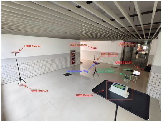
Figure 12.
Real-world experimental scene map.
As shown in Table 1, the proposed algorithm achieves higher accuracy than the ChOA, demonstrating superior localization performance. It is worth noting that, limited by the scenario layout, the localization error of the algorithm is higher than the actual localization error.

Table 1.
Algorithm operation result data table.
7. Conclusions
We present a systematic investigation of swarm intelligence optimization for solving 3D TDoA localization challenges in complex indoor environments. To address spatial outliers induced by hardware limitations and signal distortions, a novel weighted multi-beacon fusion framework is developed, which incorporates density-aware outlier filtering and weighted coordinate fusion to improve localization consistency. Through comprehensive comparisons of two metaheuristic algorithms under diverse noise conditions and spatial configurations, the proposed approach has demonstrated superior localization accuracy in resolving nonlinear hyperboloid equations compared to alternative approaches. The simulation analysis reveals the enhanced robustness of the ChOA against measurement uncertainties and environmental interference. Notably, the optimal LOF neighbor count parameter is determined according to the simulation results. Experimental results show that the proposed algorithm exhibits excellent convergence performance even under low population sizes, significantly improves the anti-interference capability against Gaussian white noise compared to baseline algorithms, and maintains anti-interference performance against multipath noise, consistent with that of baseline algorithms—though its performance is slightly inferior in handling UWB device failures. Meanwhile, the algorithm demonstrates relatively good time-lag performance and target-tracking performance, as dynamic trajectory tracking simulations establish its practical viability for continuous motion monitoring. The proposed methodology establishes a balanced optimization strategy that harmonizes algorithmic precision with operational efficiency, providing valuable insights for implementing reliable indoor localization systems in real-world applications.
Author Contributions
Conceptualization, D.M. and G.J.; Methodology, D.M. and G.J.; Software, D.M. and Y.Z.; Validation, D.M. and Y.Z.; Investigation, D.M.; Writing—original draft, D.M. and Y.Z.; Writing—review and editing, D.M., G.J. and Y.Z. All authors have read and agreed to the published version of the manuscript.
Funding
This research received no external funding.
Data Availability Statement
The data that support the findings of this study are available from the corresponding author upon reasonable request.
Conflicts of Interest
Dongfang Mao and Yun Zhao were employed by Wuxi Realid Technology Co., Ltd. The remaining authors declare that the research was conducted in the absence of any commercial or financial relationships that could be construed as a potential conflict of interest.
References
- Terças, L.; Alves, H.; de Lima, C.H.M.; Juntti, M. Bayesian-Based Indoor Factory Positioning Using AOA, TDOA, and Hybrid Measurements. IEEE Internet Things J. 2024, 11, 21620–21631. [Google Scholar] [CrossRef]
- Chen, J.F.; Zhou, B.D.; Bao, S.Q.; Liu, X.; Gu, Z.N.; Li, L.C.; Zhao, Y.P.; Zhu, J.S.; Li, Q.Q. A Data-Driven Inertial Navigation/Bluetooth Fusion Algorithm for Indoor Localization. IEEE Sens. J. 2022, 22, 5288–5301. [Google Scholar] [CrossRef]
- Gao, J.; Wu, D.Z.; Yin, F.; Kong, Q.L.; Xu, L.X.; Cui, S.G. MetaLoc: Learning to Learn Wireless Localization. IEEE J. Sel. Areas Commun. 2023, 41, 3831–3847. [Google Scholar] [CrossRef]
- Zhou, X.; Yang, Q.; Liu, Q.; Liang, W.; Wang, K.; Liu, Z.; Ma, J.; Jin, Q. Spatial–temporal federated transfer learning with multi-sensor data fusion for cooperative positioning. Inf. Fusion 2024, 105, 102182. [Google Scholar] [CrossRef]
- Ye, Y.; He, H.; Lin, E.; Tang, H. Multi-Sensor Collaborative Positioning in Range-Only Single-Beacon Systems: A Differential Chan–Gauss–Newton Algorithm with Sequential Data Fusion. Sensors 2025, 25, 2577. [Google Scholar] [CrossRef]
- Sushchenko, O.; Bezkorovainyi, Y.; Solomentsev, O.; Zaliskyi, M.; Holubnychyi, O.; Ostroumov, I.; Averyanova, Y.; Ivannikova, V.; Kuznetsov, B.; Bovdui, I.; et al. Algorithm of determining errors of gimballed inertial navigation system. In Proceedings of the International Conference on Computational Science and Its Applications, Hanoi, Vietnam, 1–4 July 2024; pp. 206–218. [Google Scholar]
- Xiong, C.; Lu, W.; Xiong, H.; Ding, H.; He, Q.; Zhao, D.; Wan, J.; Xing, F.; You, Z. Onboard cooperative relative positioning system for Micro-UAV swarm based on UWB/Vision/INS fusion through distributed graph optimization. Measurement 2024, 234, 114897. [Google Scholar] [CrossRef]
- Janczak, D.; Walendziuk, W.; Sadowski, M.; Zankiewicz, A.; Konopko, K.; Slowik, M.; Gulewicz, M. Indoor Positioning Based on Bluetooth RSSI Mean Estimator for the Evacuation Supervision System Application. IEEE Access 2024, 12, 55843–55858. [Google Scholar] [CrossRef]
- Cahyadi, W.A.; Chung, Y.H.; Adiono, T. Infrared Indoor Positioning Using Invisible Beacon. In Proceedings of the 2019 Eleventh International Conference on Ubiquitous and Future Networks (ICUFN), Split, Croatia, 2–5 July 2019; pp. 341–345. [Google Scholar]
- Gabbrielli, A.; Bordoy, J.; Xiong, W.X.; Fischer, G.K.J.; Schaechtle, T.; Wendeberg, J.; Höflinger, F.; Schindelhauer, C.; Rupitsch, S.J. RAILS: 3-D Real-Time Angle of Arrival Ultrasonic Indoor Localization System. IEEE Trans. Instrum. Meas. 2023, 72, 9600215. [Google Scholar] [CrossRef]
- Yu, D.; Li, C.G. An Accurate WiFi Indoor Positioning Algorithm for Complex Pedestrian Environments. IEEE Sens. J. 2021, 21, 24440–24452. [Google Scholar] [CrossRef]
- Jimenez Ruiz, A.R.; Seco Granja, F.; Prieto Honorato, J.C.; Guevara Rosas, J.I. Accurate Pedestrian Indoor Navigation by Tightly Coupling Foot-Mounted IMU and RFID Measurements. IEEE Trans. Instrum. Meas. 2012, 61, 178–189. [Google Scholar] [CrossRef]
- Fahama, H.S.; Ansari-Asl, K.; Kavian, Y.S.; Soorki, M.N. An Experimental Comparison of RSSI-Based Indoor Localization Techniques Using ZigBee Technology. IEEE Access 2023, 11, 87985–87996. [Google Scholar] [CrossRef]
- Shang, S.; Wang, L.X. Overview of WiFi fingerprinting-based indoor positioning. IET Commun. 2022, 16, 725–733. [Google Scholar] [CrossRef]
- Kaune, R. Accuracy studies for TDOA and TOA localization. In Proceedings of the 2012 15th International Conference on Information Fusion, Singapore, 9–12 July 2012; pp. 408–415. [Google Scholar]
- Li, X.H.; Yang, S.H. The indoor real-time 3D localization algorithm using UWB. In Proceedings of the 2015 International Conference on Advanced Mechatronic Systems (ICAMechS), Changsha, China, 1–4 November 2015; pp. 337–342. [Google Scholar]
- Kshetrimayum, R.S. An introduction to UWB communication systems. IEEE Potentials 2009, 28, 9–13. [Google Scholar] [CrossRef]
- Win, M.Z.; Scholtz, R.A. Characterization of ultra-wide bandwidth wireless indoor channels: A communication-theoretic view. IEEE J. Sel. Areas Commun. 2002, 20, 1613–1627. [Google Scholar] [CrossRef]
- Cheng, Y.; Zhou, T.Y. UWB Indoor Positioning Algorithm Based on TDOA Technology. In Proceedings of the 2019 10th International Conference on Information Technology in Medicine and Education (ITME), Qingdao, China, 23 August 2019; pp. 777–782. [Google Scholar]
- Qu, J.S.; Shi, H.N.; Qiao, N.; Wu, C.; Su, C.; Razi, A. New three-dimensional positioning algorithm through integrating TDOA and Newton’s method. EURASIP J. Wirel. Commun. Netw. 2020, 2020, 77. [Google Scholar] [CrossRef]
- Bocquet, M.; Loyez, C.; Benlarbi-Delai, A. Using enhanced-TDOA measurement for indoor positioning. IEEE Microw. Wirel. Components Lett. 2005, 15, 612–614. [Google Scholar] [CrossRef]
- Sadeghi, M.; Behnia, F.; Amiri, R. Optimal Geometry Analysis for TDOA-Based Localization Under Communication Constraints. IEEE Trans. Aerosp. Electron. Syst. 2021, 57, 3096–3106. [Google Scholar] [CrossRef]
- Yang, Y.T.; Wang, X.L.; Li, D.; Chen, D.D.; Zhang, Q.D. An Improved Indoor 3-D Ultrawideband Positioning Method by Particle Swarm Optimization Algorithm. IEEE Trans. Instrum. Meas. 2022, 71, 1005211. [Google Scholar] [CrossRef]
- Khishe, M.; Mosavi, M.R. Chimp optimization algorithm. Expert Syst. Appl. 2020, 149, 113338. [Google Scholar] [CrossRef]
- Breunig, M.M.; Kriegel, H.P.; Ng, R.T.; Sander, J. LOF: Identifying density-based local outliers. In Proceedings of the 2000 ACM SIGMOD International Conference on Management of Data, Dallas, TX, USA, 16–18 May 2000; pp. 93–104. [Google Scholar]
- Yang, X.; He, X. Bat algorithm: Literature review and applications. Int. J. Bio-Inspired Comput. 2013, 5, 141–149. [Google Scholar] [CrossRef]
- Mirjalili, S.; Mirjalili, S.M.; Lewis, A. Grey wolf optimizer. Adv. Eng. Softw. 2014, 69, 46–61. [Google Scholar] [CrossRef]
- Karaboga, D.; Akay, B. A comparative study of artificial bee colony algorithm. Appl. Math. Comput. 2009, 214, 108–132. [Google Scholar] [CrossRef]
Disclaimer/Publisher’s Note: The statements, opinions and data contained in all publications are solely those of the individual author(s) and contributor(s) and not of MDPI and/or the editor(s). MDPI and/or the editor(s) disclaim responsibility for any injury to people or property resulting from any ideas, methods, instructions or products referred to in the content. |
© 2025 by the authors. Licensee MDPI, Basel, Switzerland. This article is an open access article distributed under the terms and conditions of the Creative Commons Attribution (CC BY) license (https://creativecommons.org/licenses/by/4.0/).