A Survey of Loss Functions in Deep Learning

Abstract

Deep learning (DL), as a cutting-edge technology in artificial intelligence, has significantly impacted fields such as computer vision and natural language processing. Loss function determines the convergence speed and accuracy of the DL model and has a crucial impact on algorithm quality and model performance. However, most of the existing studies focus on the improvement of specific problems of loss function, which lack a systematic summary and comparison, especially in computer vision and natural language processing tasks. Therefore, this paper reclassifies and summarizes the loss functions in DL and proposes a new category of metric loss. Furthermore, this paper conducts a fine-grained division of regression loss, classification loss, and metric loss, elaborating on the existing problems and improvements. Finally, the new trend of compound loss and generative loss is anticipated. The proposed paper provides a new perspective for loss function division and a systematic reference for researchers in the DL field.

1. Introduction

Deep learning (DL) is a multi-layer neural network architecture that adopts an end-to-end learning mechanism to learn data features and patterns [1,2,3]. DL has been widely applied in numerous fields including computer vision and natural language processing [4,5,6].

In DL, the loss function, as the core component of the model, quantifies the deviation between model’s predicted results and ground truth (GT) and guides the adjustment of model parameters through the optimization [7,8,9,10]. In essence, it is a mathematical tool that maps the predicted error to non-negative values, thereby providing a gradient-based optimization objective function for learning [11,12,13]. A loss function is defined as follows: assume the sample sets as ${\{({\mathrm{x}}_{\mathrm{i}}, {\mathrm{y}}_{\mathrm{i}})\}}_{\mathrm{i}=1}^{\mathrm{N}}$, where x_i is the input sample, y_i is the GT, and N is the sample quantity; the model as f(x; θ), where θ is the trainable parameter, and the loss function L(θ) is shown in Equation (1).

$$(\mathrm{\theta }) = \frac{1}{\mathrm{N}}\sum _{\mathrm{i} = 1}^{\mathrm{N}}\mathrm{L}({\mathrm{y}}_{\mathrm{i}}, \mathrm{f}({\mathrm{x}}_{\mathrm{i}}; \mathrm{\theta }))$$

(1)

where $\mathrm{L}\left(\mathrm{\theta }\right)$ provides an objective measurement of the model $\mathrm{f}\left(·\right)$ by calculating the deviation between the predicted value $\mathrm{f}\left({\mathrm{x}}_{\mathrm{i}};\mathrm{\theta }\right)$ and the GT ${\mathrm{y}}_{\mathrm{i}}$.

From Equation (1), it is clear that the loss function leads the direction of model’s learning optimization, which serves as a core component of DL. Choosing an inappropriate loss function will affect the model’s effectiveness [14,15]. The mean square error (MSE) and cross-entropy loss (CE), which are provided earlier, lay the foundation of loss function [10,11]. With the increase in task complexity, new functions have been successively proposed, such as adversarial loss, triplet loss, center loss, and so on [16,17,18].

However, most research focuses on improving or constructing a novel loss function [9]. Traditionally, loss function is usually divided into regression loss and classification loss [7,8,9,19]. This division does not consider the sample interrelationships, so it is necessary to propose a new loss category, called metric loss. Unlike classification loss and regression loss that directly minimize the deviation between predicted values and GT, the optimization target of metric loss is to construct a highly discriminative embedding space through the geometric relationship between samples [20,21,22]. For example, contrast loss shortens the embedding distance of similar samples and push away dissimilar samples [18]; large-margin softmax increases the inter-class angle margin to enhance the embedding discriminability [23]. Furthermore, regression loss and classification loss calculate gradient solely dependent on continuous or discrete labels of single sample. However, metric loss requires collaborative calculation, depending on similar relationships of sample pairs, which should be parallel to regression loss and classification loss, jointly supporting the optimization requirements of DL models in complex tasks.

Therefore, this paper reclassifies and summarizes the loss function of DL and incorporates metric loss into the division. Also, it makes a more fine-grained division of regression, classification, and metric loss, elaborating on the improvement paths of these losses. Finally, the new trend of loss function, such as compound loss and generative loss, is anticipated.

The main contributions of the proposed paper are as follows:

• This proposed paper reclassifies and summarizes the loss function of DL and incorporates metric loss into the division of loss functions.
• This proposed paper makes a more fine-grained division of regression, classification, and metric loss.
• This proposed paper looks forward to new trends of loss function, including compound loss and generative loss.

The structure of this paper is as follows: This section serves as an introduction to present the main background, existing problems in the survey, and the main contributions. Section 2 will introduce regression loss, Section 3 will introduce classification loss, Section 4 will introduce metric loss, and Section 5 is the conclusion and prospects.

2. Motivation, Materials, and Methodology

This research selects the literature database Web of Science, ACM Digital Library, and ScienceDirect. The search keyword used in Web of Science is “TS = (“loss function*” OR “cost function*”) AND TS = (review OR survey) AND PY = (2015–2025).” TS means text subject. The publication year is restrained to 2015–2025. In total, 1023 papers were obtained by this keyword. Because the search results include papers in engineering, automation and control, and other fields, the research field is restrained into computer science, and 528 papers were obtained. Through a simple browsing of these 528 articles, it is found that most of them are not surveyed. Therefore, this study adds the search keyword “DT = (Review)”, which restricts the search result marked “Review” by Web of Science. The preliminary screening is to simply read the title and abstract and exclude papers that are not survey or whose topic is other, such as deep learning survey. Meanwhile, it includes a survey whose topic is loss function. A preliminary screening of 138 articles was conducted using these criteria, and a total of 6 papers were obtained. The secondary screening is to carefully read the full text, excluding loss function surveys in a single field, such as in image segmentation. Meanwhile, it includes loss function surveys in deep learning. A secondary screening of 6 articles was conducted using these criteria, and a total of 2 papers were obtained. The preliminary screening and the secondary screening are shown in

Table 1. Inclusion criteria and exclusion criteria.

Stage	Inclusion Criteria	Exclusion Criteria
preliminary screening	-it is a survey -survey topic is loss function	-not a survey -survey topic is others
secondary screening	-focus on loss function in deep learning rather than a single field	-only for loss functions in a single field, such as image segmentation

.

Since the ACM Digital Library had no subject option, we could search anywhere with the keyword “(“loss function *” OR “cost function *”) AND (“review” OR “survey”)”. The publication year is restrained to 2015–2025. A total of 12477 papers were obtained. Similar to the Web of Science, most of these are not surveyed. Therefore, this study restricts the content type to “Review”, and 533 papers were obtained. By using similar criteria in Table 1, the preliminary screening of 533 articles was conducted using these criteria, and a total of 2 papers were obtained, but there were 0 satisfactory papers found in the secondary screening.

In the “Advanced Search” interface of ScienceDirect, we selected “Title, abstract, keywords” to search. The search keyword was “(‘loss function” or “cost function”) AND (review OR survey)”. A total of 1277 papers were obtained. Because the search results included papers in engineering, mathematics, and other fields, the research field was restrained to computer science, and 335 papers were obtained. We checked the “Review article” in the “Article type” to further ensure that only surveys were retained; 72 papers were obtained. Similarly, by using criteria in Table 1, the preliminary screening of 72 papers was conducted using these criteria, and a total of 3 papers were obtained, but there were 0 satisfactory papers found in the secondary screening. The search and scan results in these three databases are shown in

Table 2. Search and screening results.

Database	Paper Volume of After Initial Search	Paper Volume of Surveys	Paper Volume After Preliminary Screening	Paper Volume After Secondary Screening
Web of Science	528	138	12	6
ACM Digital Library	12,477	533	2	0
ScienceDirect	335	72	3	0

.

Most of the existing research on loss function is to propose or improve a novel loss function, and the survey of loss function in deep learning is less and not comprehensive. Existing loss function surveys focus on a specific field, such as image segmentation. Jurdi et al. [10] summarized the loss functions of semantic segmentation based on CNN. Similarly, Shruti et al. [24] summarized some well-known loss functions widely used in image segmentation and listed the situations where using them helped the model converge faster. On the other hand, some more comprehensive surveys introduced loss functions in multiple fields. For instance, Tian et al. [11] conducted deep analysis and discussion on the loss functions in image segmentation, face recognition, and object detection within the field of computer vision. Introducing loss functions based on different fields affects the integrity of technological development and is prone to missing loss functions in cross-fields.

Meanwhile, other surveys divide loss into regression loss and classification loss. Qi et al. [7] summarized and analyzed 31 classic loss functions in deep learning, classifying loss functions into regression and classification. Similarly, Lorenzo et al. [9] also classified loss functions in the same way. Jadon et al. [8] summarized 14 regression loss functions commonly used in the time-series prediction. Terven et al. [15] conducted a comprehensive survey of loss functions and performance metrics in deep learning, dividing loss functions into regression loss and classification loss, and listed loss functions in the fields of image segmentation, face recognition, and image generation. However, this binary classification method does not consider the interrelationship of samples, and the contrast loss and a series of loss of face recognition are difficult to include in these categories. Therefore, this paper proposes a new loss category called metric loss, which constructs the loss based on the similarity between samples by distance or angle.

Specifically, this study was inspired by existing surveys, retaining some of loss function in these papers and supplementing it with papers searched and screened on Web of Science. Papers [7,8,9,15] summarize regression loss. Among them, paper [15] categorizes MSE, mean absolute error loss (MAE), Huber loss, log-cosh loss, and quantile loss as regression loss. Similarly, paper [7] also introduces these 5 regression losses. Paper [8] introduces other regression losses improved based on MSE and MAE, such as root mean squared error loss (RMSE) and root mean squared logarithmic error loss (RMSLE). RMSE performs a square root operation on MSE, while RMSLE performs a logarithmic operation on the predicted value and GT. Paper [9] introduces the above 7 losses, as well as the smooth L1 loss and balanced L1 loss improved based on Huber loss. The smooth L1 loss is a special form of Huber L1 loss, applied to the R-CNN model, while the balanced L1 loss is an improvement of the smooth L1 loss, applied to image segmentation. Furthermore, MSE and MAE originate from the basic mean bias error loss (MBE), and this study briefly introduces MBE. In essence, these 10 losses are a type of quantity difference loss, which achieves model optimization by minimizing the point-wise error between the predicted value and GT.

Regression loss is commonly used for bounding box regression in object tracking. However, bounding boxes are geometric shapes rather than single coordinate points. Quantity difference loss only penalizes the numerical error of coordinate points independently, resulting in poor regression performance for bounding boxes. Therefore, researchers initially proposed the Intersection over Union (IoU) loss, which optimizes the model by calculating the overlap between predicted bounding box and GT bounding box [25]. Subsequently, many researchers have made improvements based on IoU loss.

This study conducted a search in the Web of Science database using the keyword TS = (“Loss Function” AND “IoU” AND “Bounding Box Regression”) to obtain a total of 86 papers. The final papers were determined through two rounds of screening. The preliminary screening through reading the titles, keywords, and abstracts to eliminate some papers was conducted. These papers merely cited other people’s works and did not propose new ones. A total of 33 papers were obtained after the preliminary screening. The secondary screening through carefully reading the full texts, and a total of 8 papers were obtained. During the secondary screening, some losses specific to particular scenarios were eliminated because they did not have good generalization performance. Also, some losses with minor improvement were also eliminated. These papers consider the geometric properties of bounding boxes compared to the quantity difference loss, named geometric difference loss. The search and screening results of geometric difference loss are shown in the first row of

Table 3. The result of searching and screening in Web of Science.

Key Word	Paper Volume of After Initial Search	Paper Volume After Preliminary Screening	Paper Volume After Secondary Screening
TS = (“Loss Function” AND “IoU” AND “Bounding Box Regression”)	86	33	8
TS = (“Center Loss” AND “Improvement”)	26	8	2
TS = (“Loss Function” AND “Softmax” AND “Face recognition”)	70	21	9

.

Correspondingly, papers [7,9,15] summarize classification loss. Paper [15] categorizes binary cross-entropy loss (BCE), categorical cross-entropy loss (CCE), sparse CCE, weighted cross-entropy loss (WCE), label smoothing CE loss, poly loss, and Hinge loss as classification losses. Paper [7] categorizes 0–1 loss, Hinge loss, exponential loss, and Kullback–Leibler divergence loss as classification losses. Paper [9] introduces more comprehensive to 0–1 loss, Hinge loss, and smoothed Hinge loss, as well as BCE and CCE. Meanwhile, this paper also categorizes focal loss, dice loss, and Tversky Loss as classification losses. However, losses such as Hinge loss and exponential loss differ from cross-entropy-based losses in terms of their mathematical forms. This study categorizes the former as margin loss, which introduces marginal parameters to quantify the difference between predicted value and GT. The most typical margin loss is Hinge loss, while the smoothed hinge loss, quadratic smoothed hinge loss, and modified Huber loss, which are improvements based on hinge loss, can be categorized as margin loss.

Functions such as BCE, CCE, and focal loss are designed to make the predicted probability distribution closer to the GT distribution. In this study, they are named as probability loss. The most typical probability loss is loss based on cross-entropy. In this study, BCE, CCE, sparse CCE, WCE, BaCE, and label smoothing CE loss are categorized as probability loss. In addition, focal loss, dice loss, and Tversky Loss, as well as the log-cosh dice loss, generalized dice loss, and focal Tversky loss, which are improvements of them, are also included in this category. Probability loss also includes the poly loss and Kullback–Leibler divergence loss mentioned in [7,15].

This study proposes metric loss, which uses the similarity between samples based on their distance or angular relationship to construct an optimization objective. This study divides metric loss into Euclidean distance loss and angular margin loss. Classic contrastive loss, triplet loss, and center loss are reasonably categorized as Euclidean distance loss. Our research search on Web of Science with the keyword TS = (“Center Loss” AND “Improvement”) and obtain a total of 26 papers. After the preliminary screening, papers that cited others’ improved work were eliminated; 8 papers remained. After the secondary screening, papers that did not have generalization were eliminated; 2 papers remained. These 2 typical works were range loss [26] and center-invariant loss [27], which can be categorized into Euclidean distance loss. The search and screening results are shown in the second row of Table 3.

Angular margin loss is an improvement based on softmax loss, commonly used in face recognition. This study search on Web of Science with the keyword keywords TS = (“Loss Function” AND “Face recognition” AND “Softmax”) obtained a total of 70 papers. The preliminary screening eliminated articles that were irrelevant to the topic or cited existing works. A total of 21 papers were obtained after the preliminary screening. The secondary screening selects more typical and pioneering papers, resulting in a total of 9 papers. The search and screening for angular margin loss are shown in the third row of Table 3.

3. Regression Loss

Regression model predicts dependent variables based on values of one or more independent variables [28,29]. Let $\mathrm{f}\left(·\right)$ be a regression model governed by parameters $\mathrm{\theta }$, which maps independent variables $\mathrm{x}$, where $\mathrm{x}\in \left\{{\mathrm{x}}_0,\dots ,{\mathrm{x}}_{\mathrm{N}}\right\},{\mathrm{x}}_{\mathrm{i}}\in {ℝ}^{\mathrm{D}}$, to dependent variables $\mathrm{y}$. The model $\mathrm{f}\left(·\right)$ estimates parameters $\mathrm{\theta }$ by minimizing the loss function $\mathcal{L}$ to make predictions as close as possible to GT.

Loss functions for regression tasks are all based on the residual function, that is, the loss function is constructed from the difference between the GT $\mathrm{y}$ and the predicted value $\mathrm{f}\left(\mathrm{x}\right)$. This chapter will introduce some classic quantity difference loss, such as mean squared error loss (MSE) and mean absolute error loss (MAE) and their improvements. Furthermore, this paper specifically introduces a series of IoU-based loss used for bounding box regression in the object detection task, named geometric difference loss.

3.1. Quantity Difference Loss

Quantity difference loss directly measures the error of point-by-point value between the prediction and the GT. It guides models to approximate the value distribution by minimizing this error. The typical representative loss includes MSE and MAE, which are applicable to general regression tasks.

3.1.1. Mean Bias Error Loss (MBE)

The mean bias error loss (MBE) is a basic numerical loss function [30], which captures the average deviation in the prediction. However, it is rarely used as a loss function to train regression models as positive errors can offset negative ones, potentially causing incorrect parameter estimation. It serves as the starting point for the mean absolute error loss function and is commonly used to evaluate model performance. The mathematical formula of MBE is shown in Equation (2):

$${\mathcal{L}}_{\mathrm{MBE}} = {\displaystyle \frac{1}{\mathrm{N}}}{\displaystyle \sum }_{\mathrm{i}=1}^{\mathrm{N}}{\mathrm{y}}_{\mathrm{i}}-\mathrm{f}\left({\mathrm{x}}_{\mathrm{i}}\right),$$

(2)

where $\mathrm{N}$ is the number of samples; ${\mathrm{y}}_{\mathrm{i}}$ is the GT; and $\mathrm{f}\left({\mathrm{x}}_{\mathrm{i}}\right)$ is the predicted value. The MBE loss function curve is shown in Figure 1.

3.1.2. Mean Absolute Error Loss (MAE)

Mean absolute error loss (MAE), also known as L1 loss, is one of the most fundamental loss functions in regression tasks. It measures the average of absolute deviations in predictions [16]. The absolute value overcomes the problem that the positive error of MBE offsets the negative error. Similar to MBE, MAE is also used to evaluate the performance of the model. The mathematical formula of MAE is shown in Equation (3):

$${\mathcal{L}}_{\mathrm{MAE}} = {\displaystyle \frac{1}{\mathrm{N}}}{\displaystyle \sum }_{\mathrm{i}=1}^{\mathrm{N}}\left|{\mathrm{y}}_{\mathrm{i}}-\mathrm{f}\left({\mathrm{x}}_{\mathrm{i}}\right)\right|.$$

(3)

It should be noted that the contribution of the error follows a linear pattern, which means that small errors are as important as large ones, making the model less sensitive to outliers. MAE function curve is shown in Figure 2.

Furthermore, it can be known from Figure 2 that when the predicted value is equal to GT, the MAE function does not have tangent. The slope of the tangent to the left is $-1$, while it suddenly changes to +1 on the right. At this point, the function is non-differentiable, and there is no single definite gradient, resulting in discontinuous gradients. The sub-gradient method allows any value between −1 and 1 to be used as a sub-gradient at this point, thus enabling parameter updates to continue at these points.

Since $\left|{\mathrm{y}}_{\mathrm{i}}-\mathrm{f}\left({\mathrm{x}}_{\mathrm{i}}\right)\right|$ is the basic measure quantity in the loss, we use $\Delta \mathrm{y}=\left|{\mathrm{y}}_{\mathrm{i}}-\mathrm{f}\left({\mathrm{x}}_{\mathrm{i}}\right)\right|$ in following content.

3.1.3. Mean Squared Error Loss (MSE)

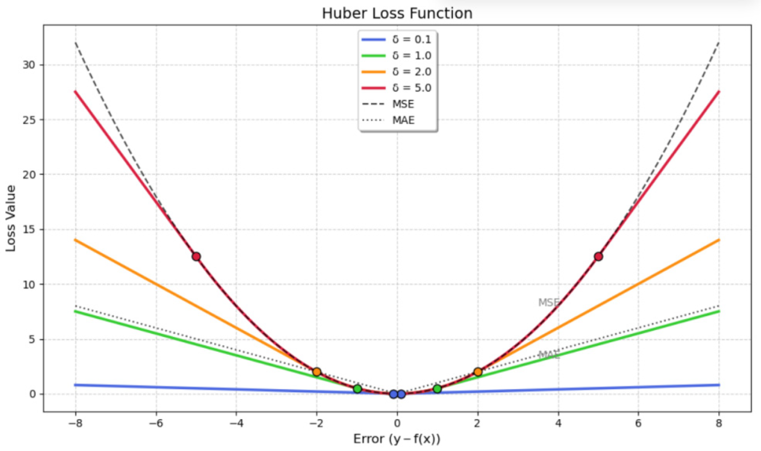
Mean squared error loss (MSE), also known as L2 loss, is the average of the squares of the differences between the predicted values and GT [16]. The square term can solve the problem of cancellation of positive and negative errors. Meanwhile, the square form can magnify larger errors, making the model pay more attention to the correction of large errors. Furthermore, the derivatives are continuous and smooth, which is convenient for the optimization of the gradient descent algorithm. The mathematical formula of MSE is shown in Equation (4):

$${\mathcal{L}}_{\mathrm{MSE}} = {\displaystyle \frac{1}{\mathrm{N}}}{\displaystyle \sum }_{\mathrm{i}=1}^{\mathrm{N}}\Delta {\mathrm{y}}^2.$$

(4)

However, MSE may be overly sensitive to outliers. Large errors can significantly increase the loss value, causing the model to be prone to overfitting outliers. The function curve of MSE is shown in Figure 3.

3.1.4. Huber Loss

Huber loss combines the advantages of MSE and MAE by using a threshold a to determine which form of loss to use [30]. When the error is less than $\mathrm{\delta }$, MSE is used. When the error is greater than $\mathrm{\delta }$, MAE is used. This makes the error linear when the difference between the model’s predicted values and GT is large. So, the Huber loss is less sensitive to outliers. Conversely, when the error is small, Huber loss follows the MSE, making convergence faster and differentiable at 0. The use of $\mathrm{\delta }$ enhances the model robustness to outliers.

The mathematical formula of Huber loss is shown in Equation (5):

$${\mathcal{L}}_{\mathrm{huber}}=\left\{\begin{array}{cc}{\displaystyle \frac{1}{2}}\Delta {\mathrm{y}}^2\hfill & \mathrm{if} \Delta \mathrm{y}\le \mathrm{\delta }\hfill \\ \mathrm{\delta }\left(\Delta \mathrm{y}-{\displaystyle \frac{1}{2}}\mathrm{\delta }\right)\hfill & \mathrm{otherwise}\hfill \end{array}\right..$$

(5)

The choice of $\mathrm{\delta }$ is crucial, and it is dynamically adjusted during training based on results. The Huber loss function curve is shown in Figure 4. Figure 4 selects four cases which $\mathrm{\delta }$ values: 0.1, 1.0, 2.0, and 5.0. The marked points are the junction between $\mathrm{\delta }$ and the equal error. The two gray curves are MAE and MSE.

3.1.5. Smooth L1 Loss

Smooth L1 loss (also known as Huber-like loss) is a special case of Huber loss and is obtained when $\mathrm{\delta }=1$. Smooth L1 loss was originally applied to the R-CNN framework [31], where it is more accurate than MSE while guaranteeing differentiability to 0. For the regression of a single coordinate, its mathematical formula is shown in Equation (6):

$${\mathcal{L}}_{\mathrm{smooth}\_\mathrm{L}1}=\left\{ \begin{array}{cc}{\displaystyle \frac{1}{2}}\Delta {\mathrm{y}}^2,\hfill & \mathrm{if} \Delta \mathrm{y}<1\hfill \\ \Delta \mathrm{y}-{\displaystyle \frac{1}{2}},\hfill & \mathrm{otherwise}\hfill \end{array}\right..$$

(6)

where ${\mathrm{y}}_{\mathrm{i}}$ is the true coordinates; $\mathrm{f}\left({\mathrm{x}}_{\mathrm{i}}\right)$ is the predicted coordinate; and $\mathrm{\beta }$ is the threshold that controls the transition between squared and linear error components.

When $\Delta \mathrm{y}<\mathrm{\beta }$, the loss function adopts the squared error form, making it smoother and more optimization-friendly for smaller errors; when $\Delta \mathrm{y}\ge \mathrm{\beta }$, it switches to the linear error form, providing more stability for larger errors and preventing the sharp increases in loss that occurs with traditional MSE. When $\mathrm{\beta }=1$, it is equivalent to smooth L1 loss.

The smooth L1 loss function curve is illustrated by the green line in Figure 4.

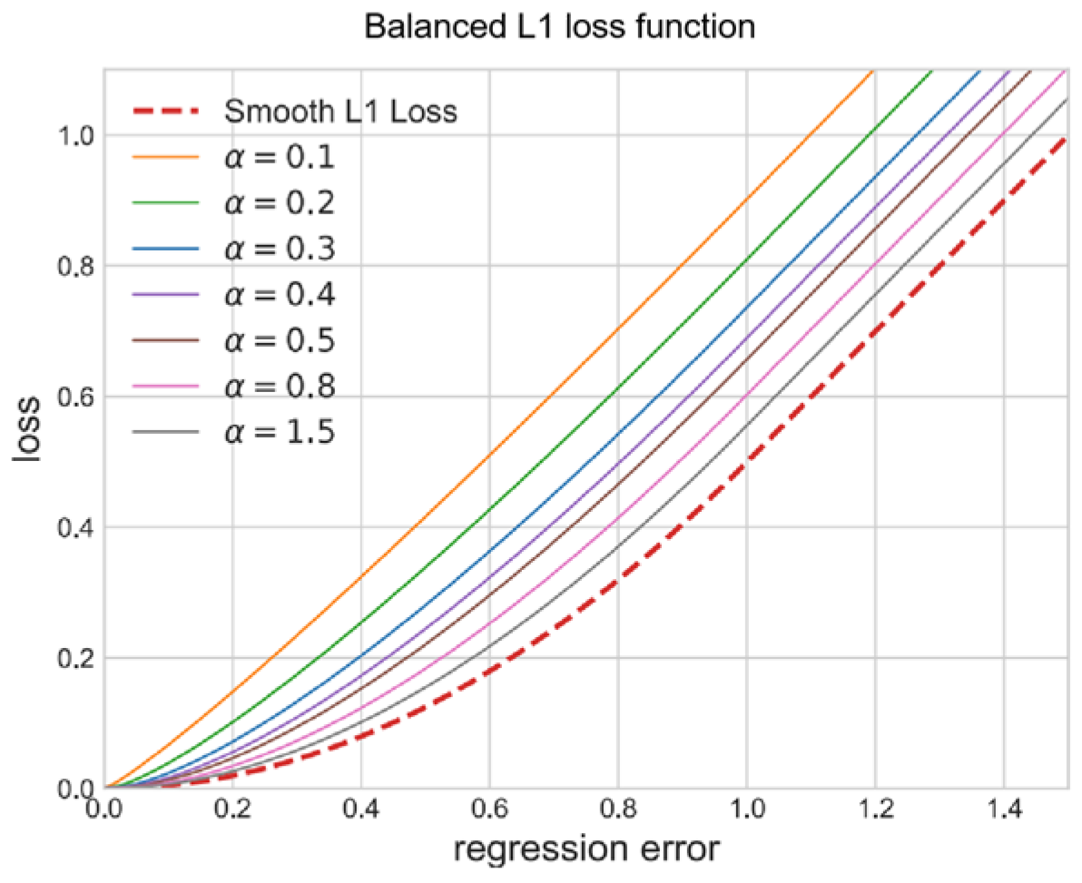
3.1.6. Balanced L1 Loss

Balanced L1 loss is an enhanced version of the standard L1 loss for bounding box regression in image segmentation. It aims to address the limitations of smooth L1 in handling sample imbalance [32]. The key idea is to introduce an inflection point to distinguish between inliers and outliers. Logarithmic functions smooth the loss gradients for inliers, while linear functions limit the gradient impact of outliers. This approach balances the contributions of easy-to-classify and hard-to-classify samples, improving training effectiveness. The mathematical formula of balanced L1 loss is shown in Equation (7):

$${\mathcal{L}}_{\mathrm{bal}\_\mathrm{L}1} = \left\{\begin{array}{c}{\displaystyle \frac{\mathrm{\alpha }}{\mathrm{b}}}\left(\mathrm{b}\Delta \mathrm{y}+1\right)\ln \left(\mathrm{b}\Delta \mathrm{y}+1\right)-\mathrm{\alpha }\Delta \mathrm{y},\mathrm{if} \Delta \mathrm{y}<1\hfill \\ \mathrm{\gamma }\Delta \mathrm{y}+\mathrm{C},\mathrm{otherwise}\hfill \end{array}\right..$$

(7)

where $\Delta \mathrm{y}$ is the regression error; $\mathrm{\alpha }$ is the parameter that controls the gradient boost for inliers; a smaller α enhances the gradient for inliers without affecting the values of outliers; the parameter $\mathrm{\gamma }$ limits the maximum gradient for outliers; $\mathrm{b}$ is a constant determined by α and $\mathrm{\gamma }$, which must satisfy $\mathrm{\alpha }\ln \left(\mathrm{b}+1\right)=\mathrm{\gamma }$; $\mathrm{C}$ is the constant term that is used to ensure that the function is continuous at $\left|{\mathrm{x}}_{\mathrm{i}}\right|=1$. The function curve of balanced L1 loss is shown in Figure 5.

3.1.7. Root Mean Squared Error Loss (RMSE)

Root mean squared error loss (RMSE) is the square root of MSE [16]. It explains the changes in the actual values and measures the average magnitude of the errors. The square root makes the penalty of RMSE for error less than that of MSE. Even if the error is large, the loss of RMSE is relatively small. The mathematical formula of RMSE is shown in Equation (8):

$${\mathcal{L}}_{\mathrm{RMSE}} = \sqrt{\frac{1}{\mathrm{N}}\sum _{\mathrm{i} = 1}^{\mathrm{N}}{\Delta \mathrm{y}}^2.}$$

(8)

However, RMSE is still a linear function, and the gradient is abrupt near the minimum. The function curve of RMSE is shown in Figure 6.

3.1.8. Root Mean Squared Logarithmic Error Loss (RMSLE)

Root mean squared logarithmic error loss (RMSLE) processes the difference between the predicted value and GT through logarithmic transformation. It is applicable to scenarios where the data has a skewed distribution or outliers [33]. The logarithmic function compresses the numerical range of large errors and reduces the impact of outliers on the overall error. Furthermore, it adopts an asymmetric punishment mechanism. When the predicted value is lower than GT, the punishment of RMSLE is more severe. When the predicted value is higher than GT, the penalty is lighter. Its mathematical formula is shown in Equation (9):

$${\mathcal{L}}_{\mathrm{RMSLE}}=\sqrt{{\displaystyle \frac{1}{\mathrm{N}}}\sum _{\mathrm{i}=1}^{\mathrm{N}}{\left(log\left({\mathrm{y}}_{\mathrm{i}}+1\right)-log\left(\mathrm{f}\left({\mathrm{x}}_{\mathrm{i}}\right)+1\right)\right)}^2},$$

(9)

where the addition of 1 before the logarithmic operation is to avoid taking the logarithm of 0, which may occur when GT or the predicted value is 0.

The function curve of RMSLE is shown in Figure 7. The GT is fixed at 10, marked with a dashed red line, while the horizontal axis represents the predicted value.

3.1.9. Log-Cosh Loss

The core idea of log-cosh loss is to smooth the predicted errors using the hyperbolic cosine function and then take the logarithm of the result as the loss value [34]. It serves a similar purpose to MSE but is less affected by significant predicted errors. The mathematical formula of log-cosh loss is shown in Equation (10):

$${\mathcal{L}}_{\log -\cosh } = \frac{1}{\mathrm{N}}\sum _{\mathrm{i} = 1}^{\mathrm{N}}\log (\cosh \Delta \mathrm{y}).$$

(10)

where $\cos \mathrm{h}\left(\mathrm{x}\right)={\displaystyle \frac{{\mathrm{e}}^{\mathrm{x}}+{\mathrm{e}}^{-\mathrm{x}}}{2}}$ is the hyperbolic cosine function.

When the error is small ($\Delta \mathrm{y}\approx 0$), the loss is $\log \left(\cos \mathrm{h}\Delta \mathrm{y}\right)\approx {\displaystyle \frac{\Delta {\mathrm{y}}^2}{2}}$, which is similar to MSE and emphasizes precise fitting. When the error is large ($\Delta \mathrm{y}>0$), the loss is $\log \left(\cos \mathrm{h}\left(\mathrm{x}\right)\right)\approx \left|{\mathrm{x}}_{\mathrm{i}}\right|-\log \left(2\right)$, which is similar to MAE and reduces sensitivity to outliers. Log-cosh loss combines the smoothness of MSE and the robustness of MAE to outliers, avoiding excessive punishment for large errors while maintaining the optimizability of the loss function. The function curve of log-cosh loss is shown in Figure 8.

3.1.10. Quantile Loss

Quantile loss is designed to predict specific quantiles (such as the median, 0.25 quantile, etc.) of the target variable rather than the mean [35]. Its mathematical form assigns different penalty weights based on the direction of the deviation between the predicted value and GT. The mathematical formula of quantile loss is shown in Equation (11):

$${\mathcal{L}}_{\mathrm{quantile}}=\left\{ \begin{array}{cc}\mathrm{\tau }\Delta \mathrm{y}\hfill & \mathrm{if} {\mathrm{y}}_{\mathrm{i}}\ge \mathrm{f}\left({\mathrm{x}}_{\mathrm{i}}\right)\hfill \\ \left(1-\tau \right)\Delta \mathrm{y}& \mathrm{otherwise}\hfill \end{array}\right.,$$

(11)

where $\mathrm{\tau }\in \left(0,1\right)$ is the target quantile, such as $\mathrm{\tau }=0.5$ for the media. When the predicted value is lower than GT, the loss weight is $\mathrm{\tau }$; otherwise, it is $1-\mathrm{\tau }$.

This asymmetry allows the model to adjust its focus on overestimation or underestimation flexibly. In the case of underestimation, the first part of the formula will dominate, and in the case of overestimation, the second part will dominate. Different penalties are given for over-prediction and under-prediction based on the chosen quantile value. The function curves of quantile loss for different $\mathrm{\tau }$ values are shown in Figure 9. Here, $\mathrm{\tau }$ takes 0.25, 0.5, and 0.75 as examples.

3.2. Geometric Difference Loss

In object detection tasks, the target of bounding box regression is to achieve geometric alignment between predicted bounding box and GT bounding box. Quantity difference loss only independently penalizes the numerical deviations of the coordinate points, ignoring their inherent geometric properties. Therefore, researchers have proposed geometric difference loss [25]. This loss directly optimizes the geometric Intersection over Union (IoU) between predicted box and GT box, which is also the core metric for evaluating detection accuracy. Geometric difference loss no longer views the coordinates as isolation but considers them as a whole geometric entity, optimizing the geometric relationship between the predicted box and the GT box.

3.2.1. Intersection over Union Loss

Intersection over Union (IoU) is a metric used in object detection to measure the overlap between two bounding boxes [36]. The mathematical formula of IoU is shown in Equation (12):

$$\mathrm{IoU}={\displaystyle \frac{\left|{\mathrm{B}}_{\mathrm{p}}\cap {\mathrm{B}}_{\mathrm{t}}\right|}{\left|{\mathrm{B}}_{\mathrm{p}}\cup {\mathrm{B}}_{\mathrm{t}}\right|}},$$

(12)

where ${\mathrm{B}}_{\mathrm{p}}$ is the predicted bounding box, ${\mathrm{B}}_{\mathrm{t}}$ is the GT bounding box, the intersection $\left|{\mathrm{B}}_{\mathrm{p}}\cap {\mathrm{B}}_{\mathrm{t}}\right|$ is the area of the overlapping part between the the ${\mathrm{B}}_{\mathrm{p}}$ and ${\mathrm{B}}_{\mathrm{t}}$, and the union $\left|{\mathrm{B}}_{\mathrm{p}}\cap {\mathrm{B}}_{\mathrm{t}}\right|$ is the total coverage area of the ${\mathrm{B}}_{\mathrm{p}}$ and ${\mathrm{B}}_{\mathrm{t}}$. The schematic diagram of IoU is shown in Figure 10.

IoU loss is a loss function widely used in object detection and image segmentation tasks. It optimizes the model by calculating the overlap degree between the coverage area of the predicted bounding box and the coverage area of the GT bounding box [25]. The loss function based on IoU is shown in Equation (13):

$${\mathcal{L}}_{\mathrm{IoU}}=1-\mathrm{IoU}.$$

(13)

This function encourages the predicted bounding box to overlap highly with the GT bounding box. A larger IoU loss value means that the predicted box is closer to the GT box, and a smaller IoU loss value means that the predicted bounding box is farther away from the GT bounding box. The IoU loss function is commonly used in single-stage detectors as part of a multi-task loss function that includes classification loss [31,37].

However, there are some limitations to the IoU loss. When the predicted box and the GT box do not overlap, that is, the IoU is 0. Also, the loss function cannot provide gradient information, resulting in optimization difficulties. However, when the predicted box and GT box overlap completely, IoU loss cannot distinguish the difference in position between the two boxes. When the shape and size of the boxes are irregular, IoU cannot effectively reflect the relative position relationship between the boxes. As a result, more loss functions based on IoU loss improvements emerge.

3.2.2. Generalized IoU (GIoU) Loss

Generalized IoU (GIoU) loss solves the problem of vanishing gradients gradient disappearance in traditional IoU without overlapping by introducing a minimum bounding rectangle $\mathcal{C}$ so that the loss function can more comprehensively reflect the difference between the predicted box and the GT box [38]. The mathematical formula of GIoU loss is shown in Equation (14):

$${\mathcal{L}}_{\mathrm{GIoU}}=1-\mathrm{IoU}+{\displaystyle \frac{\left|\mathcal{C}\setminus \left({\mathrm{B}}_{\mathrm{p}}\cup {\mathrm{B}}_{\mathrm{t}}\right)\right|}{\left|\mathcal{C}\right|}},$$

(14)

where $\mathcal{C}$ is the minimum bounding rectangle encloses both ${\mathrm{B}}_{\mathrm{p}}$ and ${\mathrm{B}}_{\mathrm{t}}$; $\left|\mathcal{C}\setminus \left({\mathrm{B}}_{\mathrm{p}}\cup {\mathrm{B}}_{\mathrm{t}}\right)\right|$ represents the area of the parts do not overlap by ${\mathrm{B}}_{\mathrm{p}}$ and ${\mathrm{B}}_{\mathrm{t}}$ within $\mathcal{C}$.

Compared with the standard IoU loss, the GIoU loss provides meaningful gradients when the two bounding boxes do not overlap at all, while the IoU loss will degrade to 0.

However, GIoU loss has a drawback in that it does not consider the aspect ratio differences between bounding boxes. This leads to situations where two boxes have a high IoU but significantly different aspect ratios, resulting in suboptimal bounding box regression, especially when objects have different shapes.

Figure 11 illustrates the differences between GIoU and IoU in various scenarios. In Figure 11, the green line indicates the GT box, the blue line indicates the predicted box, and the purple region shows the overlapping area. The gray dashed line denotes the enclosing box. The figure provides values for IoU and GIoU in three scenarios: partial overlap, non-overlap, and complete overlap. When the predicted box and GT box do not overlap, IoU is 0, but GIoU has value and can offer gradients. Conversely, when the predicted box contains the GT box or vice versa, GIoU degenerates to IoU.

3.2.3. Distance IoU (DIoU) Loss and Complete IoU (CIoU) Loss

To solve the problem of GIoU loss, the distance IoU (DIoU) loss introduces the ratio of the distance between the center points of the predicted box and the GT box to the diagonal, measuring the distance relationship of the box [39]. When the GT box contains the predicted box, DIoU loss directly measures the distance between the two boxes, making the convergence speed faster. DIoU loss can be defined in Equation (13):

$${\mathcal{L}}_{\mathrm{DIoU}}=1-\mathrm{IoU}+{\displaystyle \frac{{\mathrm{d}}^2\left({\mathrm{B}}_{\mathrm{p}},{\mathrm{B}}_{\mathrm{t}}\right)}{{\mathrm{r}}^2}},$$

(15)

where $\mathrm{d}$ is the Euclidean distance between the center of predicted box ${\mathrm{B}}_{\mathrm{p}}$ and GT box ${\mathrm{B}}_{\mathrm{t}}$, and $\mathrm{r}$ is the diagonal length of the minimum bounding rectangle enclosing both boxes.

By incorporating the distance term, DIoU loss reflects the spatial relationship between the predicted box and GT box. This is particularly useful when the boxes overlap as it can still effectively distinguish between them. However, DIoU loss only focuses on optimizing the center points and overlapping areas and does not consider the aspect ratio of the predicted box.

Figure 12 shows the losses of IoU, GIoU, and DIoU in the case of the GT box containing the predicted box. In this case, DIoU can distinguish between two boxes for its consideration of center distance, while GIoU and IoU cannot.

Reference [39] proposed the complete IoU loss (CIoU). CIoU loss is a further improved loss function based on the DIoU loss. It introduces the aspect ratio constraint to solve the problem that the aspect ratio is not considered in the DIoU loss [40]. The CIoU loss introduces a penalty term based on DIoU loss and can be defined in Equation (16):

$${\mathcal{L}}_{\mathrm{CIoU}}={\mathcal{L}}_{\mathrm{DIoU}}+\mathrm{\alpha }\cdot \mathrm{v},$$

(16)

where $\mathrm{v}$ is the penalty term of the aspect ratio of the predicted box, which is used to measure the aspect ratio difference between the predicted box and the GT box, and $\mathrm{\alpha }$ is the hyperparameter of the balance factor, which is used to control the weight of the aspect ratio penalty term. The mathematical formula of $\mathrm{v}$ is shown in Equation (17):

$$\mathrm{v}={\displaystyle \frac{4}{{\mathrm{\pi }}^2}}\left(\arctan \left({\displaystyle \frac{{\mathrm{w}}_{\mathrm{t}}}{{\mathrm{h}}_{\mathrm{t}}}}\right)-\arctan \left({\displaystyle \frac{{\mathrm{w}}_{\mathrm{p}}}{{\mathrm{h}}_{\mathrm{p}}}}\right)\right),$$

(17)

where ${\mathrm{h}}_{\mathrm{t}}$ and ${\mathrm{w}}_{\mathrm{t}}$ are the length and width of the ground-truth, and ${\mathrm{h}}_{\mathrm{p}}$ and ${\mathrm{w}}_{\mathrm{p}}$ are the length and width of the predicted box.

In Equation (17), $\mathrm{v}$ is used to measure the shape difference between the predicted box and the GT box. By quantifying the aspect ratio deviation through angle differences, the limitation that DIoU cannot distinguish different shapes when the centers coincide can be avoided. Greater difference in the aspect ratio between the predicted box and the real box means higher value of $\mathrm{v}$ and greater penalty intensity. The mathematical formula of $\mathrm{\alpha }$ is shown in Equation (18):

$$\mathrm{\alpha }={\displaystyle \frac{\mathrm{v}}{\left(1-\mathrm{IoU}\right)+\mathrm{v}}}.$$

(18)

Here, $\mathrm{\alpha }$ dynamically adjusts the contribution of the aspect ratio. In the early stage of training when the IoU is low, the center distance is optimized first. Later, when the IoU approaches 1, the focus is on adjusting the aspect ratio. The schematic diagram of CIoU when the aspect ratio of the predicted box is different is shown in Figure 13. When the aspect ratio of the predicted box is different, CIoU is sensitive to it, while IoU and DIoU are not sensitive to the aspect.

3.2.4. Efficient IoU (EIoU) Loss

Efficient IoU (EIoU) loss is based on the penalty term of CIoU loss, which separates the aspect ratio of the predicted box and the GT box, calculates the length and width of the GT box and the predicted box, respectively, and adds focal loss to focus on high-quality bounding boxes to solve the problems existing in CIoU and accelerate convergence [41]. The mathematical formula of EIoU loss is shown in Equation (19):

$${\mathcal{L}}_{\mathrm{EIoU}}={\mathcal{L}}_{\mathrm{IoU}}+{\mathrm{\lambda }}_1\cdot {\mathcal{L}}_{\mathrm{dis}}+{\mathrm{\lambda }}_2\cdot {\mathcal{L}}_{\mathrm{asp}},$$

(19)

where ${\mathcal{L}}_{\mathrm{IoU}}$ is the standard IoU loss; ${\mathcal{L}}_{\mathrm{dis}}$ is the loss of center point distance, which is used to measure the distance between the center points of two frames; ${\mathcal{L}}_{\mathrm{asp}}$ is the aspect ratio loss, used to measure the aspect ratio difference between the predicted box and the GT box; ${\mathcal{L}}_{\mathrm{dis}}$ is equal to ${\displaystyle \frac{{\mathrm{\rho }}^2\left({\mathrm{B}}_{\mathrm{p}},{\mathrm{B}}_{\mathrm{t}}\right)}{{\mathrm{c}}^2}}$, ${\mathrm{\rho }}^2\left({\mathrm{B}}_{\mathrm{p}},{\mathrm{B}}_{\mathrm{t}}\right)$ is the square of the Euclidean distance between the center point of the predicted box and the center point of the ground-truth; ${\mathcal{L}}_{\mathrm{asp}}$ is equal to ${\displaystyle \frac{{\mathrm{\rho }}^2\left({\mathrm{w}}_{\mathrm{p}},{\mathrm{w}}_{\mathrm{t}}\right)}{{\mathrm{w}}_{\mathrm{c}}^2}}+{\displaystyle \frac{{\mathrm{\rho }}^2\left({\mathrm{h}}_{\mathrm{p}},{\mathrm{h}}_{\mathrm{t}}\right)}{{\mathrm{h}}_{\mathrm{c}}^2}}$; ${\mathrm{\rho }}^2\left({\mathrm{w}}_{\mathrm{p}},{\mathrm{w}}_{\mathrm{t}}\right)$ and ${\mathrm{\rho }}^2\left({\mathrm{h}}_{\mathrm{p}},{\mathrm{h}}_{\mathrm{t}}\right),$ respectively, represent the squared differences in width and height between the predicted box and the GT box.

Furthermore, the EIoU loss directly minimizes the difference in width and length between the GT box and the predicted box, thereby achieving a faster convergence speed and better positioning effect. By independently optimizing the length and width parameters, EIoU loss avoids the gradient oscillation caused by the arctan function in CIoU loss. As shown in Figure 14, EIoU can make the width and height of the predicted box approach the GT box quickly.

3.2.5. SIoU Loss

Traditional IoU mainly focuses on the distance, overlapping area, and aspect ratio but ignores the direction alignment problem between the predicted box and the GT box. This directional deviation will lead to a slower convergence speed of the predicted box during the training process, affecting the model accuracy. SIoU introduces a direction-aware penalty term to guide the predicted box to approach the GT box quickly along the nearest coordinate axis preferentially [42]. The SIoU loss function consists of four parts: Angle Cost, Distance Cost, Shape Cost, and IoU Cost. The mathematical formula for SIoU loss is shown in Equation (20):

$${\mathcal{L}}_{\mathrm{SIoU}}=1-\mathrm{IoU}+{\displaystyle \frac{\mathrm{\Delta }+\mathrm{\Omega }}{2}},$$

(20)

where $\mathrm{\Delta }$ is distance cost, used to measure the distance between the center points of the predicted box and the GT box; $\mathrm{\Omega }$ is shape cost, used to measure the aspect ratio difference between the predicted box and the GT box, enhancing the constraint on shape similarity.

The mathematical formula for distance cost $\mathrm{\Delta }$ is shown in Equation (21):

$$\mathrm{\Delta }={\displaystyle \sum }_{\mathrm{t}=\mathrm{x},\mathrm{y}}\left(1-{\mathrm{e}}^{-{\mathrm{\gamma }\mathrm{\rho }}_{\mathrm{t}}}\right),{\mathrm{\rho }}_{\mathrm{x}}={\displaystyle \frac{\mathrm{\Delta }\mathrm{x}}{{\mathrm{\Lambda }\mathrm{w}}_{\mathrm{t}}}},{\mathrm{\rho }}_{\mathrm{y}}={\displaystyle \frac{\mathrm{\Delta }\mathrm{y}}{{\mathrm{\Lambda }\mathrm{h}}_{\mathrm{t}}}}.$$

(21)

where $\mathrm{\gamma }$ is the scaling factor of the angle weight; ${\mathrm{w}}_{\mathrm{t}}$ and ${\mathrm{h}}_{\mathrm{t}}$ are the length and width of the GT box; $\mathrm{\Delta }\mathrm{x}$ and $\mathrm{\Delta }\mathrm{y}$ are the distance between the centers of the predicted box and the GT box on the x-axis and y-axis. The mathematical formula for shape cost $\mathrm{\Omega }$ is shown in Equation (22):

$$\mathrm{\Omega }=\sum _{\mathrm{t}=\mathrm{w},\mathrm{h}}{\left(1-{\mathrm{e}}^{-{\mathrm{\omega }}_{\mathrm{t}}}\right)}^{\mathrm{\lambda }},{\mathrm{\omega }}_{\mathrm{w}}={\displaystyle \frac{\left|{\mathrm{w}}_{\mathrm{p}}-{\mathrm{w}}_{\mathrm{t}}\right|}{max\left({\mathrm{w}}_{\mathrm{p}},{\mathrm{w}}_{\mathrm{t}}\right)}},{\mathrm{\omega }}_{\mathrm{h}}={\displaystyle \frac{\left|{\mathrm{h}}_{\mathrm{p}}-{\mathrm{h}}_{\mathrm{t}}\right|}{max\left({\mathrm{h}}_{\mathrm{p}},{\mathrm{h}}_{\mathrm{t}}\right)}}.$$

(22)

where ${\mathrm{w}}_{\mathrm{p}}$ and ${\mathrm{h}}_{\mathrm{p}}$ are the length and width of the predicted box; $\mathrm{\lambda }$ is the shape penalty factor, usually set to 1, to control the intensity of the length-to-width ratio constraint.

3.2.6. Minimum Point Distance (MPD) IoU Loss

When the predicted box and GT box have the same aspect ratio but different sizes, CIoU cannot distinguish the optimization direction. Minimum point distance (MPD) IoU loss addresses this by directly minimizing the distance between the top-left and bottom-right corners of the predicted and GT box through geometric analysis [43]. It introduces a new IoU measure based on MPD and converts it into a loss function. MPD IoU is defined in Equation (23):

$$\mathrm{MPDIoU}=\mathrm{IoU}-{\displaystyle \frac{{\mathrm{d}}_1^2+{\mathrm{d}}_2^2}{{\mathrm{w}}^2+{\mathrm{h}}^2}},$$

(23)

where ${\mathrm{d}}_1$ and ${\mathrm{d}}_2$ are the Euclidean distance between the upper-left corner point and the lower-right corner point of the predicted box and the GT box; $\mathrm{w}$ and $\mathrm{h},$ respectively, represent the width and length of the input image and are used to normalize the distance term. Figure 15 illustrates the illustrated diagrams of ${\mathrm{d}}_1$ and ${\mathrm{d}}_2$ and $\mathrm{w}$ and $\mathrm{h}$.

The MPD IoU loss directly optimizes the coordinates of the upper left and lower right corners of the predicted box and the GT box and achieves more accurate geometric alignment by minimizing the Euclidean distance between the two pairs of key points. The mathematical formula of the MPD IoU loss is shown in Equation (24):

$${\mathcal{L}}_{\mathrm{MPDIoU}}=1-\mathrm{MPDIoU}.$$

(24)

The MPD IoU only needs to calculate the Euclidean distances between the top-left and bottom-right corners of the predicted box and GT box. Without the need to calculate the width and height penalty terms that are split like EIoU or the angle parameters like CIoU, it significantly reduces the computational complexity. Meanwhile, when the predicted box and GT box share the same aspect ratio but differ in scale, the CIoU/EIoU loss provides no useful gradient; however, the MPD IoU reflects size differences by minimizing corner point distances, and it is more suitable for real-time detection models.

3.2.7. Pixel-IoU (PIoU) Loss

Pixel-IoU (PIoU) loss is a loss function specially designed for rotating target detection, aiming to solve the problem of angular error in the traditional rotation box regression [44]. PIoU loss directly takes pixel-level IoU calculation as the optimization objective and achieves derivability through approximation methods. It solves the complex problem of IoU calculation for rotating frames and enhances the sensitivity to shape and angle. The mathematical formula for PIoU loss is shown in Equation (25):

$${\mathcal{L}}_{\mathrm{PIoU}}=-{\displaystyle \frac{1}{\left|\mathrm{M}\right|}}\sum _{\left({\mathrm{B}}_{\mathrm{p}},{\mathrm{B}}_{\mathrm{t}}\right)\in \mathrm{M}}lnPIoU\left({\mathrm{B}}_{\mathrm{p}},{\mathrm{B}}_{\mathrm{t}}\right).$$

(25)

where $\mathrm{PIoU}\left({\mathrm{B}}_{\mathrm{p}},{\mathrm{B}}_{\mathrm{t}}\right)$ is the pixel-level intersection and union ratio of the predicted box and the GT box; $\mathrm{M}$ is the set of positive sample pairs, defined as the matching pairs where IoU ≥ 0.5. As shown in Figure 16, an example of PIoU loss is presented.

3.2.8. Alpha-IoU Loss

Alpha-IoU loss adjusts the loss weights for different IoU values by tuning the parameter $\mathrm{\alpha }$ to enhance the detection ability of the model for high IoU and low IoU targets [45]. For instance, when $\mathrm{\alpha }>1$, the loss function focuses more on high-IoU targets, whereas when $\mathrm{\alpha }<1$, it becomes more sensitive to low-IoU targets. The mathematical formula for Alpha-IoU loss is shown in Equation (26):

$${\mathcal{L}}_{\mathrm{AlphaIoU}}=={\displaystyle \frac{1}{\mathrm{\alpha }}}\left(1-{\mathrm{IoU}}^{\mathrm{\alpha }}\right),$$

(26)

where $\mathrm{\alpha }$ is a power parameter, usually taking a value greater than 0, used to control the sensitivity of losses to high IoU targets. When $\mathrm{\alpha }>1$, the loss and gradient of the high IoU target are enhanced to improve the positioning accuracy.

3.2.9. Inner-IoU Loss

The Inner-IoU loss adaptively optimizes the regression process of different IoU samples by dynamically adjusting the scale of the auxiliary bounding box [46]. It generates auxiliary bounding boxes through the ratio to replace the original bounding boxes for IoU calculation. First, introduce the ratio to generate the boundary coordinates of the auxiliary box; this is shown in Equation (27):

$$\begin{array}{c}{\mathrm{b}}_{\mathrm{l}}^{\mathrm{gt}}={\mathrm{x}}_{\mathrm{c}}^{\mathrm{gt}}-{\displaystyle \frac{{\mathrm{w}}^{\mathrm{gt}}\cdot \mathrm{ratio}}{2}}, {\mathrm{b}}_{\mathrm{r}}^{\mathrm{gt}}={\mathrm{x}}_{\mathrm{c}}^{\mathrm{gt}}+{\displaystyle \frac{{\mathrm{w}}^{\mathrm{gt}}\cdot \mathrm{ratio}}{2}}\\ {\mathrm{b}}_{\mathrm{t}}^{\mathrm{gt}}={\mathrm{y}}_{\mathrm{c}}^{\mathrm{gt}}-{\displaystyle \frac{{\mathrm{h}}^{\mathrm{gt}}\cdot \mathrm{ratio}}{2}}, {\mathrm{b}}_{\mathrm{b}}^{\mathrm{gt}}={\mathrm{y}}_{\mathrm{c}}^{\mathrm{gt}}+{\displaystyle \frac{{\mathrm{h}}^{\mathrm{gt}}\cdot \mathrm{ratio}}{2}}\\ {\mathrm{b}}_{\mathrm{l}}={\mathrm{x}}_{\mathrm{c}}-{\displaystyle \frac{\mathrm{w}\cdot \mathrm{ratio}}{2}}, {\mathrm{b}}_{\mathrm{r}}={\mathrm{x}}_{\mathrm{c}}+{\displaystyle \frac{\mathrm{w}\cdot \mathrm{ratio}}{2}}\\ {\mathrm{b}}_{\mathrm{t}}={\mathrm{y}}_{\mathrm{c}}-{\displaystyle \frac{\mathrm{h}\cdot \mathrm{ratio}}{2}}, {\mathrm{b}}_{\mathrm{b}}={\mathrm{y}}_{\mathrm{c}}+{\displaystyle \frac{\mathrm{h}\cdot \mathrm{ratio}}{2}}\end{array},$$

(27)

where $\left({\mathrm{x}}_{\mathrm{c}}^{\mathrm{gt}},{ \mathrm{y}}_{\mathrm{c}}^{\mathrm{gt}}\right)$ is the center point of the ground-truth, and the width and length are, respectively, ${\mathrm{w}}^{\mathrm{gt}}$ and ${\mathrm{h}}^{\mathrm{gt}}$; $\left({\mathrm{x}}_{\mathrm{c}},{ \mathrm{y}}_{\mathrm{c}}\right)$ is the center point of the ground-truth predicted box, and the width and length are, respectively, $\mathrm{w}$ and $\mathrm{h}$; ${\mathrm{b}}_{\mathrm{l}}$, ${\mathrm{b}}_{\mathrm{r}}$, ${\mathrm{b}}_{\mathrm{t}}$, and ${\mathrm{b}}_{\mathrm{b}}$ represent the left boundary, right boundary, upper boundary, and lower boundary of the predicted auxiliary box.

Similarly, ${\mathrm{b}}_{\mathrm{l}}^{\mathrm{gt}}$, ${\mathrm{b}}_{\mathrm{r}}^{\mathrm{gt}}$, ${\mathrm{b}}_{\mathrm{t}}^{\mathrm{gt}}$, and ${\mathrm{b}}_{\mathrm{b}}^{\mathrm{gt}}$ represent the boundary of the real auxiliary box. $\mathrm{ratio}>1$ represents magnification, and $\mathrm{ratio}<1$ indicates shrinking. The descriptions of the meanings of each symbol of Inner-IoU are shown in Figure 17.

The formula of Inner-IoU is shown in Equation (28):

$${\mathrm{IoU}}^{\mathrm{inner}}={\displaystyle \frac{\mathrm{inter}}{\mathrm{union}}},$$

(28)

where $\mathrm{inter}$ is shown in Equation (29):

$$\mathrm{inter}=\left(\min \left({\mathrm{b}}_{\mathrm{r}}^{\mathrm{gt}},{\mathrm{b}}_{\mathrm{r}}\right)-\max \left({\mathrm{b}}_{\mathrm{l}}^{\mathrm{gt}},{\mathrm{b}}_{\mathrm{l}}\right)\right)\times \left(\min \left({\mathrm{b}}_{\mathrm{b}}^{\mathrm{gt}},{\mathrm{b}}_{\mathrm{b}}\right)-\max \left({\mathrm{b}}_{\mathrm{t}}^{\mathrm{gt}},{\mathrm{b}}_{\mathrm{t}}\right)\right),$$

(29)

and $\mathrm{union}$ is shown in Equation (30):

$$\mathrm{union}=\left({\mathrm{w}}^{\mathrm{gt}}{\mathrm{h}}^{\mathrm{gt}}+\mathrm{wh}\right)\cdot {\mathrm{ratio}}^2-\mathrm{inter}.$$

(30)

The Inner-IoU loss can be seamlessly integrated into existing IoU variants. Taking CIoU as an example, the formula of the Inner-CIoU loss is shown in Equation (31):

$${\mathcal{L}}_{\mathrm{InnerIoU}}={\mathcal{L}}_{\mathrm{CIoU}}+\mathrm{IoU}-{\mathrm{IoU}}^{\mathrm{inner}}.$$

(31)

The Inner-IoU loss can achieve dynamic gradient adjustment. For high IoU samples with nearly completed target positioning, a smaller auxiliary box is used to increase the absolute value of the gradient and accelerate convergence. For low IoU samples with large initial positioning deviations, a larger auxiliary box is used to expand the effective regression range and avoid gradient vanishing. Furthermore, Inner-IoU does not require modification of the model structure and can directly replace the existing IoU losses, achieving plug-and-play.

4. Classification Loss

The goal of classification is to assign a certain class label from $\mathrm{C}$ discrete classes to the input $\mathrm{x}$ [47,48,49]. Similar to regression, classification trains the parameters $\mathrm{\theta }$ of the model $\mathrm{f}$ by minimizing loss function. Classification includes binary classification and multi-classification. For binary classification, the value of $\mathrm{f}\left(\mathrm{x}\right)$ is $\left\{0,1\right\}$, where 0 represents the negative class, and 1 represents the positive class. For the output of the sigmoid function, ${\mathrm{f}}_{\mathrm{c}}$ represents the probability that the model $\mathrm{f}$ predicts the sample belongs to the positive class. For multi-classification problems, 0 indicates that the sample does not belong to the category $\mathrm{c}$. Similarly, for the output obtained by normalizing the softmax function, ${\mathrm{f}}_{\mathrm{c}}\left(\mathrm{x}\right)\in \left[0,1\right]$, it represents the probability that the model predicts the sample belongs to the category $\mathrm{c}$.

Classification loss can be divided into margin loss and probability loss. Margin loss introduces margin parameter to quantify difference between predicted value and GT, forcing the model to maintain a safe distance between the predicted value and the decision boundary on the basis of correct classification [50,51]. Probability loss improves the generalization ability of the classification model by optimizing the accuracy of probability prediction [52,53].

4.1. Margin Loss

4.1.1. Zero-One Loss

The most fundamental and intuitive margin loss is the zero-one loss [54]. It takes 1 when the predicted value is different from GT; otherwise, it takes 0, as shown in Equation (32):

$${\mathcal{L}}_{\mathrm{zero}\_\mathrm{one}}=\left\{\begin{array}{cc}1& \mathrm{if} \mathrm{f}\left(\mathrm{x}\right)\cdot \mathrm{y}<0\hfill \\ 0\hfill & \mathrm{otherwise}\hfill \end{array}\right..$$

(32)

This kind of loss directly reflects the classification error rate, but it is overly sensitive to outliers and lacks convexity and differentiability. Thus, it cannot be used directly. However, the usable loss can be derived based on the zero-one loss. So, it is the basis of other margin loss. The function curve of zero-one loss is shown in Figure 18.

4.1.2. Hinge Loss

Hinge loss is often used in support vector machines (SVMs) [54] to optimize the model by penalizing the gap between the predicted values and GT. Its mathematical formula is shown in Equation (33):

$${\mathcal{L}}_{\mathrm{hinge}}=\max \left(0, 1-\left(\mathrm{f}\left(\mathrm{x}\right)\cdot \mathrm{y}\right)\right).$$

(33)

It can be known from this formula that there is a loss only when the product of the predicted value and GT is less than 1. This forces the model to maintain a margin of at least 1 on the basis of correct classification. In this way, penalties are only imposed on samples that are misclassified or have insufficient intervals, making the model pay more attention to the overall error rather than individual samples. However, this loss is non-differentiable at $\mathrm{f}\left(\mathrm{x}\right)\cdot \mathrm{y}=1$; the gradient is discontinuous. The function curve of hinge loss is shown in Figure 19.

4.1.3. Smoothed Hinge Loss

To address the non-smoothness issue of hinge loss, smoothed hinge loss achieves continuous differentiability through smoothing processing, realizes more stable gradient descent, and optimizes training stability [55]. Its mathematical formula is shown in Equation (34):

$${\mathcal{L}}_{\mathrm{smoothed}\_\mathrm{hinge}}=\left\{\begin{array}{cc}0\hfill & \mathrm{if} 1-\mathrm{f}\left(\mathrm{x}\right)\cdot \mathrm{y}\le 0\hfill \\ {\displaystyle \frac{{\left(1-\mathrm{f}\left(\mathrm{x}\right)\cdot \mathrm{y}\right)}^2}{2\mathrm{\alpha }}}\hfill & \mathrm{if} 0<1-\mathrm{f}\left(\mathrm{x}\right)\cdot \mathrm{y}\le \mathrm{\alpha }\hfill \\ \left(1-\mathrm{f}\left(\mathrm{x}\right)\cdot \mathrm{y}\right)-{\displaystyle \frac{\mathrm{\alpha }}{2}}& \mathrm{if} 1-\mathrm{f}\left(\mathrm{x}\right)\cdot \mathrm{y}>\mathrm{\alpha }\hfill \end{array}\right.,$$

(34)

where $\mathrm{\alpha }$ is the smoothing parameter, which controls the width of the smooth area. This loss is continuous and second-order differentiable at $\mathrm{f}\left(\mathrm{x}\right)\cdot \mathrm{y}=1$; has no loss at $\mathrm{f}\left(\mathrm{x}\right)\cdot \mathrm{y}\le 1$; has smoothly transitions with a quadratic function at $1<\mathrm{f}\left(\mathrm{x}\right)\cdot \mathrm{y}\le 1+\mathrm{\alpha }$; and maintains a linear penalty at $\mathrm{f}\left(\mathrm{x}\right)\cdot \mathrm{y}>1+\mathrm{\alpha }$, similar to the original hinge loss.

The function curve of smoothed hinge loss is shown in Figure 20. In Figure 20, $\mathrm{\alpha }$ takes 1.0. The green line and the red line represent the boundary line.

4.1.4. Quadratic Smoothed Hinge Loss

Another common variant of hinge loss is the quadratic smoothed hinge loss, which is globally second-order differentiable and suitable for scenarios requiring second-order optimization [56]. Its mathematical formula is shown in Equation (35):

$${\mathcal{L}}_{\mathrm{Qsmoothed}\_\mathrm{hinge}}=\left\{\begin{array}{cc}{\displaystyle \frac{1}{2\mathrm{\gamma }}}\max {(0,1-\left(\mathrm{f}\left(\mathrm{x}\right)\cdot \mathrm{y}\right))}^2\hfill & \left(\mathrm{f}\left(\mathrm{x}\right)\cdot \mathrm{y}\right)>=1-\mathrm{\gamma }\hfill \\ 1-{\displaystyle \frac{\mathrm{\gamma }}{2}}-\left(\mathrm{f}\left(\mathrm{x}\right)\cdot \mathrm{y}\right)\hfill & \mathrm{otherwise}\hfill \end{array}\right.,$$

(35)

where the hyperparameters $\mathrm{\gamma }$ determine the degree of smoothness.

When $\mathrm{\gamma }$ approaching 0, the loss becomes the original hinge loss. The function curve of quadratic smoothed hinge loss is shown in Figure 21. In this figure, the case of taking $\mathrm{\gamma }=0.5$ and $\mathrm{\gamma }=1.0$ is shown.

4.1.5. Modified Huber Loss

Modified Huber loss is a minor variation of the regression Huber loss and is a special case of the quadratic smooth hinge loss when $\mathrm{\gamma }=2$ [56]. The function curve of the modified Huber loss is shown in Figure 22. In this figure, the red line represents modified Huber loss, and the green line and blue line are the same as the lines in Figure 21.

4.1.6. Exponential Loss

The background of exponential loss can be traced back to the proposal of the AdaBoost algorithm. AdaBoost dynamically adjusts the sample weights so that in each round of iteration, higher weights are assigned to the samples with classification errors, thereby paying more attention to these hard samples in the subsequent training. This mechanism enables AdaBoost to perform well in noisy datasets or imbalanced datasets. Exponential loss, as the objective function of AdaBoost, is originally designed to amplify the influence of classification errors through exponential penalties [57]. Thereby, it guides the model to gradually improve the classification performance. The mathematical formula of exponential loss is shown in Equation (36):

$${\mathcal{L}}_{\mathrm{exponential}}=\exp \left(-\left(\mathrm{f}\left(\mathrm{x}\right)\cdot \mathrm{y}\right)\right).$$

(36)

The function curve of the exponential loss is shown in Figure 23.

4.2. Probability Loss

The probability loss function quantifies the difference between predicted probability distribution and true data distribution, making the predicted probability distribution approaches to the true data distribution through the optimization process. Given the observational data $\mathcal{D}={\left\{\left({\mathrm{x}}_{\mathrm{i}},{\mathrm{y}}_{\mathrm{i}}\right)\right\}}_{\mathrm{i}=1}^{\mathrm{N}}$, where ${\mathrm{x}}_{\mathrm{i}}\in \mathrm{X}$, ${\mathrm{x}}_{\mathrm{i}}$ is the input, ${\mathrm{y}}_{\mathrm{i}}\in \mathrm{Y}$, ${\mathrm{y}}_{\mathrm{i}}$ is the true output, which is the discrete classification label. Set the model ${\mathrm{f}}_{\mathrm{\theta }}\left(·\right)$ and adjust it by parameters $\mathrm{\theta }$. Set ${\mathrm{p}}_{\mathrm{i}}={\mathrm{f}}_{\mathrm{\theta }}\left({\mathrm{x}}_{\mathrm{i}}\right)$ as the predicted probability distribution where the sample is of the positive category. The target of the probability loss function is to find the optimal parameters so as to minimize the difference between the predicted probability distribution by the model and the true data distribution.

4.2.1. Binary Cross-Entropy Loss (BCE)

The cross-entropy (CE) originated from information entropy and is used to measure the difference between predicted probability distribution and GT probability distribution [17,58]. CE is well suited for probabilistic models because it turns the intuitive idea “give high probability to what actually happened” into a concrete number. When the predicted probability assigned to the correct result is already high, the loss stays low, and when it is low, the loss rises sharply. Therefore, CE is used for classification tasks in deep neural networks.

BCE is the application of cross-entropy in binary classification scenarios [59] and is applicable to tasks with labels of 0 or 1. The formula of BCE is shown in Equation (37):

$${\mathcal{L}}_{\mathrm{BCE}}=-{\displaystyle \frac{1}{\mathrm{N}}}\sum _{\mathrm{i}=1}^{\mathrm{N}}\left[{\mathrm{y}}_{\mathrm{i}}log\left({\mathrm{p}}_{\mathrm{i}}\right)+\left(1-{\mathrm{y}}_{\mathrm{i}}\right)log\left(1-{\mathrm{p}}_{\mathrm{i}}\right)\right],$$

(37)

where $\mathrm{N}$ is the sample size, ${\mathrm{y}}_{\mathrm{i}}$ is GT, ${\mathrm{y}}_{\mathrm{i}}\in \left\{0,1\right\},$ and ${\mathrm{p}}_{\mathrm{i}}$ is the predicted probability of the model pair, ${\mathrm{p}}_{\mathrm{i}}={\mathrm{f}}_{\mathrm{\theta }}\left({\mathrm{x}}_{\mathrm{i}}\right)$.

The BCE is intuitive and easy to implement. As the maximum likelihood estimation objective, the gradient of BCE is directly proportional to the prediction error due to its own design characteristics. The larger the error is, the stronger the gradient is. It helps to alleviate the problem of gradient disappearance. Thus, during the training process, it provides stable gradient updates, which favor the model convergence. However, in datasets with category imbalance, BCE will cause the model to bias a certain category and ignore the features of a minority of categories. Assuming GT is category 1, the loss function curve of BCE is shown in Figure 24.

4.2.2. Categorical Cross-Entropy Loss (CCE)

CCE expands the binary classification scenarios and handles multi-classification problems [60]. Let ${\mathrm{p}}_{\mathrm{i}}$ be the predicted probability distribution of samples, ${\mathrm{p}}_{\mathrm{i}}=\left[{\mathrm{p}}_{\mathrm{i},1},\dots ,{\mathrm{p}}_{\mathrm{i},\mathrm{c}}\right]$. The mathematical formula of CCE is shown in Equation (38):

$${\mathcal{L}}_{\mathrm{CCE}}=-{\displaystyle \frac{1}{\mathrm{N}}}\sum _{\mathrm{i}=1}^{\mathrm{N}}\sum _{\mathrm{c}=1}^{\mathrm{C}}{\mathrm{y}}_{\mathrm{i},\mathrm{c}}log\left({\mathrm{p}}_{\mathrm{i},\mathrm{c}}\right),$$

(38)

where $\mathrm{C}$ is the number of categories; $\mathrm{N}$ is the total number of samples; ${\mathrm{y}}_{\mathrm{i},\mathrm{c}}$ is GT; and ${\mathrm{p}}_{\mathrm{i},\mathrm{c}}$ is the probability that the model predicts the sample $\mathrm{i}$ belongs to the category $\mathrm{c}$. In model training, minimization ${\mathcal{L}}_{\mathrm{CCE}}$ makes ${\mathrm{p}}_{\mathrm{i},\mathrm{c}}$ close to 1 for category $\mathrm{c}$ and close to 0 for other categories.

In neural networks, models usually output normalized results through the softmax function. A softmax function is shown in Equation (39):

$${\mathrm{p}}_{\mathrm{i},\mathrm{c}}={\displaystyle \frac{exp\left({\mathrm{z}}_{\mathrm{i},\mathrm{c}}\right)}{{\sum }_{\mathrm{k}=1}^{\mathrm{C}}exp{\left({\mathrm{z}}_{\mathrm{i},\mathrm{k}}\right)}^{\prime }}},$$

(39)

where ${\mathrm{z}}_{\mathrm{i},\mathrm{c}}$ and ${\mathrm{z}}_{\mathrm{i},\mathrm{k}}$ are the inputs of a neuron.

4.2.3. Sparse Categorical Cross-Entropy Loss

Sparse categorical cross-entropy loss (sparse CCE) is applicable to the situation where the category label is an integer rather than a unique hot vector [60]. Its mathematical formula is shown in Equation (40):

$${\mathcal{L}}_{\mathrm{SparseCCE}}=-{\displaystyle \frac{1}{\mathrm{N}}}\sum _{\mathrm{i}=1}^{\mathrm{N}}log\left({\mathrm{p}}_{\mathrm{i},{\mathrm{y}}_{\mathrm{i}}}\right)$$

(40)

where ${\mathrm{p}}_{\mathrm{i},{\mathrm{y}}_{\mathrm{i}}}$ is the probability assigned to the correct class ${\mathrm{y}}_{\mathrm{i}}$.

Compared with CCE with one hot coding, sparse CCE has higher computational efficiency, but it is lacking in representation granularity. Sparse CCE directly represents the label with a single real number (such as ${\mathrm{y}}_{\mathrm{i}}=3.0$) instead of storing entire one hot encoding (such as ${\mathrm{y}}_{\mathrm{i}}=\left[0,0,0,1,0\dots \dots \right]$), which improves the computational efficiency. However, sparse real number labels compress categories into a continuous dimensional space, resulting in a limited number of categories that can be clearly distinguished, while one hot coding can distinguish any number of categories by assigning higher dimensions to each category. Thus, compared with sparse CCE, CCE with one hot coding has advantages in fine-grained large-scale classification.

4.2.4. Weighted Cross-Entropy Loss (WCE)

BCE and CCE are sensitive to category imbalance. When there are more samples of a certain category in the dataset and fewer samples of other categories, the model may ignore a minority category [60]. WCE introduces category weights on the basis of CE to adjust the contribution of different categories to the total loss [61]. By allocating weights to different categories, the model’s focus on minority categories or key categories is enhanced, which is particularly suitable for data scenarios with imbalanced categories. The mathematical formula of binary WCE is shown in Equation (41):

$${\mathcal{L}}_{\mathrm{BWCE}}=-{\displaystyle \frac{1}{\mathrm{N}}}\sum _{\mathrm{i}=1}^{\mathrm{N}}\left({\mathrm{wy}}_{\mathrm{i}}log\left({\mathrm{p}}_{\mathrm{i}}\right)+\left(1-{\mathrm{y}}_{\mathrm{i}}\right)log\left(1-{\mathrm{p}}_{\mathrm{i}}\right)\right)$$

(41)

where $\mathrm{w}$ is the weight applied to the positive category samples; ${\mathrm{y}}_{\mathrm{i}}$ represents GT, ${\mathrm{y}}_{\mathrm{i}}\in \left\{0,1\right\}$. ${\mathrm{y}}_{\mathrm{i}}=0$ represents a negative category, and ${\mathrm{y}}_{\mathrm{i}}=1$ represents positive category. ${\mathrm{p}}_{\mathrm{i}}$ represents the probability distribution predicted by the model, ${\mathrm{p}}_{\mathrm{i}}\in \left(0,1\right)$.

In multi-classification scenarios, each label is assigned a weight based on its frequency or importance. Then, calculate a binary WCE term for each label and sum it up. The mathematical formula for multi-classification WCE is shown in Equation (42):

$${\mathcal{L}}_{\mathrm{CWCE}}=-{\displaystyle \frac{1}{\mathrm{N}}}\sum _{\mathrm{i}=1}^{\mathrm{N}}\sum _{\mathrm{c}=1}^{\mathrm{C}}{\mathrm{w}}_{\mathrm{c}}·{\mathrm{y}}_{\mathrm{i},\mathrm{c}}log\left({\mathrm{p}}_{\mathrm{i},\mathrm{c}}\right),$$

(42)

where $\mathrm{C}$ is the total number of categories, and ${\mathrm{w}}_{\mathrm{c}}$ is the weight of the category $\mathrm{c}$.

WCE helps ensure that a minority category has sufficient influence on the gradient during the training process and reduces the model’s bias towards the majority classes.

Figure 25 shows the function curve of the binary WCE. Figure 25 presents a two-graph display. The left graph shows the loss curves under different positive sample weights when the GT is 1, and the right graph shows the loss curves under different negative sample weights when GT is 0. At the same time, four weight values were adopted, namely, 0.5, 1.0, 2.0, and 5.0.

4.2.5. Balanced Cross-Entropy Loss (BaCE)

BaCE [61] is similar to WCE. It proposes that not only the positive class samples should be weighted but also the negative class samples are very important. The formula for the equilibrium cross-entropy of binary classification is shown as Equation (43):

$${\mathcal{L}}_{\mathrm{BaCE}}=-{\displaystyle \frac{1}{\mathrm{N}}}\sum _{\mathrm{i}=1}^{\mathrm{N}}\left({\mathrm{wy}}_{\mathrm{i}}log\left({\mathrm{p}}_{\mathrm{i}}\right)+(1-\mathrm{w})\left(1-{\mathrm{y}}_{\mathrm{i}}\right)log\left(1-{\mathrm{p}}_{\mathrm{i}}\right)\right),$$

(43)

where $\mathrm{w}$ is the weights of the positive class.

4.2.6. Label Smoothing Cross-Entropy Loss (Label Smoothing CE Loss)

Label smoothing CE loss improves the traditional cross-entropy loss by introducing label smoothing technology [62]. It replaces the real labels of one-hot encoding with soft labels, that is, by transferring part of the probability quality from GT to other categories, thereby reducing the model’s overconfidence in a single category. The formula obtained by smoothing the label is shown in Equation (44):

$${\tilde{\mathrm{y}}}_{\mathrm{i},\mathrm{c}}=\left(1-\mathrm{ϵ}\right){\mathrm{y}}_{\mathrm{i},\mathrm{c}}+{\displaystyle \frac{\mathrm{ϵ}}{\mathrm{C}}},$$

(44)

where $\mathrm{ϵ}$ is the smoothing factor, $\mathrm{ϵ}\in \left[0,1\right]$. The typical value $\mathrm{ϵ}$ range from 0.05 to 0.2. Regulation $\mathrm{ϵ}$ can be achieved by verifying performance.

The mathematical formula of label smoothing CE is shown in Equation (45):

$${\mathcal{L}}_{\mathrm{label}\_\mathrm{SmoothCE}}=-\sum _{\mathrm{c}=1}^{\mathrm{C}}{\tilde{\mathrm{y}}}_{\mathrm{i},\mathrm{c}}log\left({\mathrm{p}}_{\mathrm{i},\mathrm{c}}\right).$$

(45)

After smoothing, the model does not allow a probability of 1 to be assigned to any single category. Label smoothing can prevent overconfident predictions. Empirical evidence indicates that label smoothing helps the model avoid overfitting on noisy data or unrepresentative training samples. As shown in Figure 26, it presents the comparison of the function curves between label smoothing CE and standard CE. Figure 26 shows the situation where the predicted probability value is higher than 0.5. When the predicted probability approaches 1, CE gradually approaches 0, while label smoothing CE does not approach 0 but converges to a fixed value.

4.2.7. Focal Loss

Focal loss is a loss function designed for the problem of category imbalance, used to solve the problem of imbalance in the number of positive class samples and negative class samples. It reduces the weight of easy-to-classify samples by adjusting parameters, enabling the model to focus more on learning hard-to-classify samples [63]. For binary classification problems, the mathematical formula of focal loss is shown in Equation (46):

$${\mathcal{L}}_{\mathrm{focal}}=-{\displaystyle \frac{1}{\mathrm{N}}}\sum _{\mathrm{i}=1}^{\mathrm{N}}{\mathrm{\alpha }}_{\mathrm{t}}{\left(1-{\mathrm{p}}_{\mathrm{t}}\right)}^{\mathrm{\gamma }}log\left({\mathrm{p}}_{\mathrm{t}}\right)$$

(46)

where ${\mathrm{p}}_{\mathrm{t}}$ is the predicted probability of the model for the correct category, and ${\mathrm{\alpha }}_{\mathrm{t}}$ is a hyperparameter and a category balance factor, used to balance the weights of positive and negative samples. When the proportion of positive samples is relatively small, a balance factor can be set to increase the loss contribution of positive samples; $\mathrm{\gamma }$ is the focusing parameter. When $\mathrm{\gamma }\ge 0$, the loss controls the weight distribution of easy-to-classify and hard-to-classify samples; when $\mathrm{\gamma }=0$, focal loss degenerates into WCE. When $\mathrm{\gamma }$ increases, the loss contribution of easy-to-classify samples will be significantly suppressed, forcing the model to focus on hard-to-classify samples.

The function curves of focal loss are shown in Figure 27. Curves with the five values of 0, 0.5, 1, 2, and 5 are plotted, respectively. It can be seen from Figure 27 that as $\mathrm{\gamma }$ increases, the loss of the easy-to-classify samples is compressed smaller, the relative weight of the hard-to-classify samples increases, and the curve becomes steeper in the low-probability area.

4.2.8. Gradient Harmonizing Mechanism (GHM) Loss

In the single-stage target detector, there exists the problem of imbalance in the gradient distribution of easy and hard samples, that is, a large number of easy samples will dominate the gradient update. However, the traditional loss based on CE merely alleviates the class imbalance by adjusting the loss weights but does not fully consider the dynamic balance at the gradient level. For this purpose, Li et al. proposed GHM loss [64]. GHM loss dynamically adjusts the weight loss of the sample through gradient density. It is divided into classification task loss (GHM-C) and regression task loss (GHM-R). The mathematical formula of GHM-C is shown in Equation (47):

$${\mathcal{L}}_{\mathrm{GHM}-\mathrm{C}}=\sum _{\mathrm{i}=1}^{\mathrm{N}}{\displaystyle \frac{{\mathcal{L}}_{\mathrm{CE}}\left({\mathrm{p}}_{\mathrm{i}},{\mathrm{y}}_{\mathrm{i}}\right)}{\mathrm{GD}\left({\mathrm{g}}_{\mathrm{i}}\right)}},$$

(47)

where ${\mathrm{g}}_{\mathrm{i}}=\left|{\mathrm{p}}_{\mathrm{i}}-{\mathrm{y}}_{\mathrm{i}}\right|$ is the gradient norm, representing the deviation between the predicted probability and GT. $\mathrm{GD}\left({\mathrm{g}}_{\mathrm{i}}\right)$ is gradient density, which defined as the number of samples within a unit gradient modulus interval. It is used to measure the density of the gradient distribution.

The gradient density $\mathrm{GD}\left(\mathrm{g}\right)$ is obtained by statistically counting the number of samples between intervals of the gradient modulus. The mathematical formula of gradient density is shown in Equation (48):

$$\mathrm{GD}\left(\mathrm{g}\right)={\displaystyle \frac{1}{{\mathrm{l}}_{\mathrm{e}}\left(\mathrm{g}\right)}}\sum _{\mathrm{k}=1}^{\mathrm{N}}{\mathrm{\delta }}_{\mathrm{e}}\left({\mathrm{g}}_{\mathrm{k}},\mathrm{g}\right),$$

(48)

where ${\mathrm{\delta }}_{\mathrm{e}}$ is the indicator function, which determines whether the sample gradient belongs to the current interval. ${\mathrm{l}}_{\mathrm{e}}\left(\mathrm{g}\right)$ is the length of the interval.

GHM automatically reduces the weight of easy samples (i.e., the gradient modulus is close to 0 or 1) based on the gradient density while enhancing the contribution of moderately hard samples, avoiding the training being dominated by a large number of simple, and maintaining the dynamic balance of the gradient.

As shown in Figure 28, the gradient norm adjustment effect using GHM-C, CE and focal loss is demonstrated. Specifically, the horizontal coordinate of Figure 28 is the original gradient norm, representing the gradient size caused by the difference between the model’s predicted values and GT. The vertical coordinate is the reconstructed gradient norm, representing the gradient size adjusted by GHM-C, CE, and focal loss. It can be known from Figure 28 that GHM-C effectively suppresses the overly strong gradient signals of easy samples, avoids the overfitting noise of the model, and at the same time retains the key gradient signals of hard samples to prevent training collapse.

4.2.9. Class-Balanced Loss

Cui et al. proposed the theory of effective number of samples, introduced the category balance term, and dynamically adjusted the loss weights to solve the category imbalance problem in long-tail datasets [65]. The category balance term is defined in Equation (49):

$${\mathrm{E}}_{\mathrm{n}}={\displaystyle \frac{1-{\mathrm{\beta }}^{\mathrm{n}}}{1-\mathrm{\beta }}},$$

(49)

where $\mathrm{n}$ is the number of samples in the true category, and $\mathrm{\beta }\in \left[0,1\right)$ is a hyperparameter to control the attenuation rate of data coverage. From this formula, it can be known that when $\mathrm{\beta }=1$, valid samples ${\mathrm{E}}_{\mathrm{n}}\to 0$, that is, all samples are independent information. Similarly, when $\mathrm{\beta }=0,$ the valid samples ${\mathrm{E}}_{\mathrm{n}}\to 1$, that is, all samples were completely overlapping, which is equivalent to the traditional weighting strategy. The meaning of this formula is that as the number of samples increases, the information gain brought by the new samples gradually decreases.

Figure 29 shows the relationship between the number of samples in the true category and the category balance term under different $\mathrm{\beta }$ values. As can be seen from Figure 29, with the increase in $\mathrm{\beta }$, the curve begins to tilt downward. This indicates that the category balance term corresponding to the category with a large number of samples decreases, thereby reducing the weight of the large sample category when calculating the loss. In particular, when $\mathrm{\beta }$ is approaching 1, the category equilibrium term of the curve approaches 1 when the sample size is very small, but as the sample size increases, the category equilibrium term drops sharply, indicating a strong inhibitory effect on categories with a large sample size.

The class-balanced loss adjusts the weights inversely proportional to the number of valid samples. Its mathematical formula is shown in Equation (50):

$${\mathcal{L}}_{\mathrm{CB}}={\displaystyle \frac{1}{{\mathrm{E}}_{\mathrm{n}}}}\cdot {\mathcal{L}}_{\mathrm{base}},$$

(50)

where ${\mathcal{L}}_{\mathrm{base}}$ is the basic loss function, such as CE or focal loss.

The class-balanced loss is modeled through the effective sample size to avoid the extreme imbalance caused by simple inverse frequency weighting and is more in line with the actual coverage of the data distribution. Furthermore, the class-balanced loss can be integrated into multiple loss functions.

4.2.10. Dice Loss

Dice loss originates from the dice coefficient index, which measures the similarity between two sets and is often used in the field of image segmentation. To better understand, this subsection takes the image segmentation task as an example. In image segmentation, dice coefficient is used to evaluate the degree of overlap between the predicted segmentation mask and the true segmentation mask. The dice coefficient is defined as the size of the intersection of the predicted segmentation mask and the true segmentation mask divided by their sum [66]. The formula of dice coefficient is shown in Equation (51):

$$\mathrm{Dice} \mathrm{Coefficient}={\displaystyle \frac{2\left|\mathrm{P}\cap \mathrm{Y}\right|}{\left|\mathrm{Y}\right|+\left|\mathrm{P}\right|}},$$

(51)

where $\mathrm{Y}$ is the binary segmentation mask predicted by the model. In the mask matrix, 1 represents the target region, 0 represents the background, and $\mathrm{Y}$ represents the predicted segmentation region; $\mathrm{P}$ is the binary segmentation mask of GT, representing the true segmentation region. The values range from 0 to 1, where 0 indicates no overlap between the two regions, and 1 indicates complete overlap.

The visualization of dice coefficient is shown in Figure 30.

Dice loss changes from this metric [67], which calculates the overlapping part between the predicted region and the true region. In tasks with relatively scarce foreground categories, such as in lesion detection or other small target scenarios, dice–based loss achieves a classification loss better than the pixel level by directly optimizing the spatial overlap between the predicted region and the real region. The mathematical formula of dice loss is shown in Equation (52):

$${\mathcal{L}}_{\mathrm{Dice}}=1-\mathrm{Dice} \mathrm{Coefficient}=1-{\displaystyle \frac{2\cdot \sum \left({\mathrm{p}}_{\mathrm{i}}{\mathrm{y}}_{\mathrm{i}}\right)+\mathrm{ϵ}}{\sum {\mathrm{p}}_{\mathrm{i}}+\sum {\mathrm{y}}_{\mathrm{i}}+\mathrm{ϵ}}},$$

(52)

where ${\mathrm{p}}_{\mathrm{i}}$ is the predicted probability value of the model for the $\mathrm{i}$-th pixel, ${\mathrm{y}}_{\mathrm{i}}$ is the true probability value of the $\mathrm{i}$-th pixel, and $\mathrm{ϵ}$ is the smoothing coefficient to prevent the denominator from being zero and causing numerical instability and, at the same time, alleviate the gradient vanishing problem of extreme prediction. $\sum \left({\mathrm{p}}_{\mathrm{i}}{\mathrm{y}}_{\mathrm{i}}\right)$ is the intersection part of the predicted region and GT region and represents the sum of the total pixels of the predicted region and GT region.

In fact, in binary classification problems, the dice coefficient is mathematically equivalent to F1–score, and the dice coefficient can be transformed into Equation (53):

$$\mathrm{Dice} \mathrm{Coefficient}={\displaystyle \frac{2\mathrm{TP}}{2\mathrm{TP}+\mathrm{FP}+\mathrm{FN}}}=\mathrm{F}1,$$

(53)

where TP (the true-positive sample) refers to the number of positive examples correctly identified by the model. FP (the false-positive sample) refers to the number of negative examples that the model mistakenly judges as positive examples. TN (the true-negative sample) is the number of negative examples correctly identified by the model. FN (the false-negative sample) refers to the number of positive examples that the model misses. These four indicators together constitute the core of the confusion matrix.

The F1score provides a balanced measure between precision and recall rate and is suitable for cases of category imbalance. Similarly, the dice loss measures the degree of overlap by calculating the ratio of the intersection of two sets to the union, which can balance the accuracy and recall rate.

4.2.11. Log-Cosh Dice Loss

Dice loss has the problem of non-convexity, which may lead to instability in the optimization process when training imbalanced datasets. Therefore, Jadon et al. proposed the log-cosh dice loss [24], which enhances its smoothness and robustness by wrapping the log-cosh function outside the dice loss. The mathematical formula of log-cosh dice loss is shown in Equation (54):

$${\mathcal{L}}_{\mathrm{logcosh}\_\mathrm{dice}}=\log \left(\cosh \left({\mathcal{L}}_{\mathrm{Dice}\_\mathrm{L}}\right)\right),$$

(54)

where $\cos \mathrm{h}\left(·\right)$ is a hyperbolic cosine function, which defined as $\cos \mathrm{h}\left(\mathrm{x}\right)={\displaystyle \frac{{\mathrm{e}}^{\mathrm{x}}+{\mathrm{e}}^{-\mathrm{x}}}{2}}$. The derivative tanh of the log-cosh function is a smooth function within the range $\pm 1$.

The introduction of the log-cosh function makes the loss function smoother when the predicted values are far from the GT values, avoids the sharp fluctuations of the dice loss in extreme cases, and has better robustness against outliers and noise. Furthermore, due to its smoothness, the log-cosh dice loss is more suitable for optimization algorithms, such as the gradient descent method, thereby improving the convergence speed and stability of the model.

4.2.12. Generalized Dice Loss

Although the dice loss can solve the category imbalance problem to a certain extent, it is not applicable to severe category imbalance problems. Generalized dice loss is an extension of the traditional dice loss to address the shortcomings of the traditional dice loss when dealing with imbalanced datasets. Sudre et al. proposed a generalized dice loss, which adjusted the contributions of different categories by introducing weights, thereby handling imbalanced datasets more effectively [68]. The generalized dice loss is shown in Equation (55):

$${\mathcal{L}}_{\mathrm{g}\_\mathrm{dice}}=1-{\displaystyle \frac{2{\sum }_{\mathrm{c}=1}^{\mathrm{C}}{\sum }_{\mathrm{i}=1}^{\mathrm{N}}{\mathrm{w}}_{\mathrm{l}}{\mathrm{y}}_{\mathrm{i},\mathrm{c}}{\mathrm{p}}_{\mathrm{i},\mathrm{c}}}{{\sum }_{\mathrm{c}=1}^{\mathrm{C}}{\sum }_{\mathrm{i}=1}^{\mathrm{N}}{\mathrm{w}}_{\mathrm{l}}\left({\mathrm{y}}_{\mathrm{i},\mathrm{c}}+{\mathrm{p}}_{\mathrm{i},\mathrm{c}}\right)}},$$

(55)

where ${\mathrm{w}}_{\mathrm{l}}$ is the weight, usually defined as ${\mathrm{w}}_{\mathrm{l}}={\displaystyle \frac{1}{{\sum }_{\mathrm{i}=1}^{\mathrm{N}}{{\mathrm{y}}_{\mathrm{i},\mathrm{c}}}^2}}$.

4.2.13. Tversky Loss

Tversky loss is designed for the problem of category imbalance and performs particularly well in image segmentation. It achieves flexible control of different misclassification costs by adjusting the penalty weights of FP and FN [69]. Its core formula is based on the Tversky index (TI), and the basic Tversky index is shown as Equation (56):

$$\mathrm{TI}={\displaystyle \frac{\left|\mathrm{P}\cap \mathrm{Y}\right|}{\left|\mathrm{P}\cap \mathrm{Y}\right|+\mathrm{\alpha }\left|\mathrm{P}\backslash \mathrm{Y}\right|+\mathrm{\beta }\left|\mathrm{Y}\backslash \mathrm{P}\right|}},$$

(56)

where $\mathrm{P}$ is the predicted mask of the model, $\mathrm{Y}$ is GT, with $\mathrm{P}\cap \mathrm{Y}$ representing TP, that is, the number of pixels where the predicted region overlaps with the GT region; $\mathrm{P}-\mathrm{Y}$ is FP, that is, the number of pixels predicted to be positive but actually negative; $\mathrm{Y}-\mathrm{P}$ is FN, that is, the number of pixels predicted to be negative but actually positive; $\mathrm{\alpha } \mathrm{and} \mathrm{\beta }$ are the hyperparameter for adjusting FP and FN. Another form of expression is shown in Figure 31.

The Tversky loss is defined in Equation (57):

$${\mathcal{L}}_{\mathrm{Tversky}}=1-\mathrm{TI}= {\displaystyle \frac{{{\displaystyle \sum }}_{\mathrm{i}=1}^{\mathrm{N}}{ \mathrm{p}}_{\mathrm{i}}{\mathrm{y}}_{\mathrm{i}}}{{{\displaystyle \sum }}_{\mathrm{i}=1}^{\mathrm{N}}{ \mathrm{p}}_{\mathrm{i}}{\mathrm{y}}_{\mathrm{i}}+\mathrm{\alpha }{{\displaystyle \sum }}_{\mathrm{i}=1}^{\mathrm{N}}{ \mathrm{p}}_{\mathrm{i}}{\mathrm{y}}_{\mathrm{i}}+\mathrm{\beta }{{\displaystyle \sum }}_{\mathrm{i}=1}^{\mathrm{N}}{ \mathrm{p}}_{\mathrm{i}}{\mathrm{y}}_{\mathrm{i}}}}.$$

(57)

When $\mathrm{\alpha }=\mathrm{\beta }=0.5$, the Tversky loss was equivalent to the dice loss. It is applicable in situations where it is necessary to balance false positives and false negatives. When dealing with highly imbalanced datasets, the values $\mathrm{\alpha }$ and $\mathrm{\beta }$ will be adjusted according to the requirements, to prioritize reducing the impact of a certain type of error. If the impact of FN is greater, set $\mathrm{\alpha }>\mathrm{\beta }$ and increase the penalties for false negatives. If the impact of FP is greater, set $\mathrm{\alpha }<\mathrm{\beta }$ to increase the penalties for false positives.

4.2.14. Focal Tversky Loss

Focal Tversky loss is an improved loss that combines Tversky loss and focal loss [70], aiming to enhance the model’s ability to focus on small targets or difficult samples. Focal Tversky loss introduces the concept of focal loss on the basis of Tversky loss and enhances the focus on difficult samples by adjusting parameters. The mathematical formula of focal Tversky loss is shown in Equation (58):

$${\mathcal{L}}_{\mathrm{FTversky}}=\sum _{\mathrm{c}}{(1-\mathrm{TI})}^{{\displaystyle \frac{1}{\mathrm{\gamma }}}},$$

(58)

where $\mathrm{TI}$ is the Tversky index, and $\mathrm{\gamma }$ is the modulation parameter and controls the degree of focus on hard samples. Larger values of $\mathrm{\gamma }$ will make the model pay more attention to samples with a lower Tversky index, thereby improving the recognition ability for fewer samples.

Figure 32 shows the influence of different $\mathrm{\gamma }$ values on the focal Tversky loss. As the Tversky index increases, the overlap between the prediction and reality increases, and the loss decreases. The larger $\mathrm{\gamma }$ is, the faster the curve drops, meaning that a stronger suppression is applied to samples with a high Tversky index, that is, those with better predictions, thereby paying more attention to hard samples.

4.2.15. Sensitivity Specificity Loss

Sensitivity-specificity loss is a loss that solves the problem of category imbalance by balancing the penalty weights of FN and FP [71]. The core idea is to combine the two indicators of sensitivity and specificity (also known as recall rate) and adjust the degree of concern of the model for missed detection and false detection through a weighting mechanism. In image segmentation, sensitivity is defined in Equation (59):

$$\mathrm{Specifity}={\displaystyle \frac{{\sum }_{\mathrm{i}=1}^{\mathrm{N}}{\left({\mathrm{y}}_{\mathrm{i}}-{\mathrm{p}}_{\mathrm{i}}\right)}^2\left(1-{\mathrm{y}}_{\mathrm{i}}\right)}{{\sum }_{\mathrm{i}=1}^{\mathrm{N}}\left(1-{\mathrm{y}}_{\mathrm{i}}\right)+\mathrm{ϵ}}}.$$

(59)

Specificity is defined in Equation (60):

$$\mathrm{Sensitivity}={\displaystyle \frac{{\sum }_{\mathrm{i}=1}^{\mathrm{N}}{\left({\mathrm{y}}_{\mathrm{i}}-{\mathrm{p}}_{\mathrm{i}}\right)}^2}{{\sum }_{\mathrm{i}=1}^{\mathrm{N}}{\mathrm{y}}_{\mathrm{i}}+\mathrm{ϵ}}}.$$

(60)

The sensitivity-specificity loss formula is defined in Equation (61):

$${\mathcal{L}}_{\mathrm{SSloss}}=\mathrm{w}·{\displaystyle \frac{{\sum }_{\mathrm{i}=1}^{\mathrm{N}}{\left({\mathrm{y}}_{\mathrm{i}}-{\mathrm{p}}_{\mathrm{i}}\right)}^2}{{\sum }_{\mathrm{i}=1}^{\mathrm{N}}{\mathrm{y}}_{\mathrm{i}}+\mathrm{ϵ}}}+(1-\mathrm{w})·{\displaystyle \frac{{\sum }_{\mathrm{i}=1}^{\mathrm{N}}{\left({\mathrm{y}}_{\mathrm{i}}-{\mathrm{p}}_{\mathrm{i}}\right)}^2\left(1-{\mathrm{y}}_{\mathrm{i}}\right)}{{\sum }_{\mathrm{i}=1}^{\mathrm{N}}\left(1-{\mathrm{y}}_{\mathrm{i}}\right)+\mathrm{ϵ}}},$$

(61)

where $\mathrm{w}$ is the weight parameter, which is used to control the trade-off between sensitivity and specificity; $\mathrm{ϵ}$ is the smoothness coefficient. This formula strikes a balance between sensitivity and specificity by adjusting the weight parameters $\mathrm{w}$. When $\mathrm{w}$ approaches 0, the model pays more attention to improving specificity; when $\mathrm{w}$ approaches 1, the model pays more attention to improving the sensitivity.

4.2.16. Poly Loss

Poly loss is a loss function framework designed from the perspective of polynomial expansion, inspired by Taylor expansion [72]. This framework allows for flexible adjustment of the importance of different polynomial bases by representing the loss as a linear combination of polynomial. Thereby it can adapt to the requirements of different tasks and datasets. The traditional CE and focal loss are special cases of poly loss, and poly loss provides a more general perspective to redesign and understand these losses. The general form of poly loss is expressed in Equation (62):

$${\mathcal{L}}_{\mathrm{polyloss}}=-\sum _{\mathrm{n}=1}^{\mathrm{N}}{\mathrm{\alpha }}_{\mathrm{n}}{\left(1-{\mathrm{p}}_{\mathrm{t}}\right)}^{\mathrm{n}}$$

(62)

where ${\mathrm{p}}_{\mathrm{t}}$ is the predicted probability of the true category $\mathrm{t}$ of a single sample, and ${\mathrm{\alpha }}_{\mathrm{n}}$ is the coefficient of the polynomial of the $\mathrm{n}$-th term and controls the contribution size of each term ${\left(1-{\mathrm{p}}_{\mathrm{t}}\right)}^{\mathrm{n}}$. Larger $\mathrm{n}$ will make losses more sensitive to minor deviations of ${\mathrm{p}}_{\mathrm{t}}$.

A simplified form of poly loss is the poly-1 loss, and its mathematical formula is expressed in Equation (63):

$${\mathcal{L}}_{\mathrm{polyloss}}=\mathrm{CE}\left(\mathrm{y}, \hat{\mathrm{p}}\right)+\mathrm{ϵ}\left(1-{\mathrm{p}}_{\mathrm{t}}\right),$$

(63)

where $\mathrm{CE}\left(·\right)$ is the basic cross-entropy loss, and $\mathrm{ϵ}$ is a hyperparameter. Setting $\mathrm{ϵ}=0$ makes the Poly-1 loss return to the basic cross-entropy loss. When $\mathrm{ϵ}>0$, the term $\mathrm{ϵ}\left(1-{\mathrm{p}}_{\mathrm{t}}\right)$ imposes a greater penalty for credible incorrect predictions, which can alleviate overfitting.

Figure 33 reveals the differences between poly loss and focal loss in the design of the loss. The black dotted line represents the changing trend of the polynomial coefficients. In the poly loss framework, focal loss can only move the polynomial coefficients horizontally (indicated by the green arrow), while the proposed poly loss framework is more universal. It also allows for vertical adjustment of the polynomial coefficients of each polynomial term (indicated by the red arrow).

4.2.17. Kullback–Leibler Divergence Loss

Kullback–leibler divergence (KL divergence loss) is mainly used to measure the difference between two probability distributions and is often applied in fields such as generative models (such as GANs), variational autoencoders (VAEs), and reinforcement learning [73]. For example, in generative adversarial networks (GANs), the KL divergence loss is used to reward the degree of proximity between the embedding vectors generated by the generator and the prior distribution. For discrete distributions, the definition of KL divergence loss is shown in Equation (64):

$${\mathcal{L}}_{\mathrm{kl}}={\mathrm{D}}_{\mathrm{KL}}(\mathrm{P}\parallel \mathrm{Q})=\sum _{\mathrm{x}}\mathrm{P}\left(\mathrm{x}\right)log\left({\displaystyle \frac{\mathrm{P}\left(\mathrm{x}\right)}{\mathrm{Q}\left(\mathrm{x}\right)}}\right),$$

(64)

where $\mathrm{P}\left(\mathrm{x}\right)$ is the true distribution, and $\mathrm{Q}\left(\mathrm{x}\right)$ is the predicted distribution by the model, that is, the distribution that needs to be optimized.

It should be noted that the KL divergence does not satisfy symmetry, which is ${\mathrm{D}}_{\mathrm{KL}}\left(\mathrm{P}\parallel \mathrm{Q}\right)\ne$ ${\mathrm{D}}_{\mathrm{KL}}\left(\mathrm{Q}\parallel \mathrm{P}\right)$. Therefore, in practical applications, it is necessary to determine which distribution should be used as the true distribution based on specific problems. Figure 34 shows the KL divergence between two Gaussian distributions. The horizontal axis of this graph represents the values of random variables, and the vertical axis represents the probability density. In the figure, there are two curves, where red represents $\mathrm{P}\left(\mathrm{x}\right)$, blue represents $\mathrm{Q}\left(\mathrm{x}\right)$, pink area represents ${\mathrm{D}}_{\mathrm{KL}}\left(\mathrm{P}\parallel \mathrm{Q}\right)$, and blue area represents ${\mathrm{D}}_{\mathrm{KL}}\left(\mathrm{Q}\parallel \mathrm{P}\right)$. The asymmetry of KL divergence can be seen from Figure 34.

5. Metric Loss

Metric learning maps the input data to the embedding space by learning a customized distance metric function so that the distance between similar samples in this space is reduced as much as possible and the distance between dissimilar samples is increased as much as possible. Correspondingly, the metric loss is the loss based on metric learning, aiming to guide the model to learn a high-quality, generalizable embedding space or feature representation. This type of loss hopes that the feature vectors of similar samples in the embedding space are highly similar (i.e., the distance between the vectors is small), while the feature vectors of dissimilar samples should be significantly different (i.e., the distance between the vectors is large). This kind of loss usually serves similar metric tasks, such as face verification, image retrieval, or anomaly detection [74,75,76], etc. The final predicted value is often accomplished by calculating the similarity of feature vectors and making threshold judgments. The similarity calculation of vectors can be directly achieved through the calculation of vector distances or the included angles between vectors, which is commonly known as cosine similarity. According to the different metrics for calculating similarity in the embedding space, the losses based on feature embedding can be divided into two categories: the Euclidean distance loss and the angular margin loss.

5.1. Euclidean Distance Loss

The loss based on Euclidean distance is a metric learning method [75], which is a loss that directly takes the geometric distance in the embedding space as the optimization target. It attempts to decrease the distance of similar samples in the embedding space and increase the distance of dissimilar samples in the embedding space, thereby achieving the training and parameter adjustment of the model. The mathematical formula of the Euclidean distance is shown in Equation (65):

$$\mathrm{D}\left({\mathrm{x}}^1,{\mathrm{x}}^2\right) = {({\mathrm{x}}^1-{\mathrm{x}}^2)}^{\top }\left({\mathrm{x}}^1-{\mathrm{x}}^2\right) = \parallel {\mathrm{x}}^1-{\mathrm{x}}^2{\parallel }_2,$$

(65)

where ${\mathrm{x}}^1 \mathrm{and} {\mathrm{x}}^2$ are the feature vectors of two samples in the vector space.

Contrastive loss, triplet loss, and center loss are commonly used in Euclidean distance loss.

5.1.1. Contrastive Loss

The core idea of contrastive loss is to enhance the discriminative ability of the model by optimizing the relative distance between samples. Specifically, the target of contrastive loss is to make positive sample pairs of the same category as close as possible in the embedding space, while negative sample pairs of different categories are as far apart as possible [18,76,77]. The mathematical formula of contrastive loss is shown in Equation (66):

$${\mathcal{L}}_{\mathrm{contrastive}}=\sum _{\mathrm{i}=1}^{\mathrm{N}}\left[{\mathrm{y}}_{\mathrm{i}}·{∥{\mathrm{x}}_{\mathrm{i}}^1-{\mathrm{x}}_{\mathrm{i}}^2∥}_2^2+\left(1-{\mathrm{y}}_{\mathrm{i}}\right)·max{\left(0,\mathrm{m}-{∥{\mathrm{x}}_{\mathrm{i}}^1-{\mathrm{x}}_{\mathrm{i}}^2∥}_2\right)}^2\right],$$

(66)

where ${\parallel {\mathrm{x}}_{\mathrm{i}}^1-{\mathrm{x}}_{\mathrm{i}}^2\parallel }_2$ is the Euclidean distance between the samples ${\mathrm{x}}_{\mathrm{i}}^1{ \mathrm{and} \mathrm{x}}_{\mathrm{i}}^2$; ${\mathrm{y}}_{\mathrm{i}}$ is a label indicating whether a sample pair belongs to the same category, ${\mathrm{y}}_{\mathrm{i}}\in \left\{0,1\right\}$. If it belongs to the same category, ${\mathrm{y}}_{\mathrm{i}}$ is 1; if not, ${\mathrm{y}}_{\mathrm{i}}$ is 0. Set $\mathrm{m}$ as the margin. If ${\mathrm{x}}_{\mathrm{i}}^1{ \mathrm{and} \mathrm{x}}_{\mathrm{i}}^2$ are positive sample pairs, it is hoped that their Euclidean distance is as small as possible. If ${\mathrm{x}}_{\mathrm{i}}^1{ \mathrm{and} \mathrm{x}}_{\mathrm{i}}^2$ are negative sample pairs, it is hoped that their Euclidean distance is greater than the margin.

Contrastive loss is trained through pairwise input. For example, in the face recognition task, the model will simultaneously receive two images as input samples. When the two samples come from the same person, we give label ${\mathrm{y}}_{\mathrm{i}}=1$. Otherwise, the given label ${\mathrm{y}}_{\mathrm{i}}=0$. When ${\mathrm{y}}_{\mathrm{i}}=1$, the corresponding loss is ${\mathcal{L}}_{\mathrm{contrastive}}={\displaystyle \frac{1}{2}}\parallel {\mathrm{x}}_{\mathrm{i}}^1-{\mathrm{x}}_{\mathrm{i}}^2{\parallel }_2^2,$ and when ${\mathrm{y}}_{\mathrm{i}}=0$, the corresponding loss is ${\mathcal{L}}_{\mathrm{contrastive}}={\displaystyle \frac{1}{2}}\max {(0,\mathrm{m}-{\parallel {\mathrm{x}}_{\mathrm{i}}^1-{\mathrm{x}}_{\mathrm{i}}^2\parallel }_2)}^2$. On the one hand, the smaller the Euclidean distance of the same samples in the embedding space, the smaller the loss value, ensuring the similarity of samples from the same person. On the other hand, the greater the Euclidean distance of different samples in the embedding space, the smaller the loss value, ensuring the differences of samples from different personnel. Furthermore, set a margin $\mathrm{m}$. If the distances of negative sample pairs from different people are included, the model will generate loss, thereby increasing the distances of negative sample pairs and causing them to separate. Therefore, the contrastive loss achieves the pairwise matching degree and also effectively trains the feature extraction model. Figure 35 shows the effect of contrastive loss, bringing similar samples closer and pushing different samples farther away.

The classic work by using contrastive loss is the DeepID series of networks. DeepID2 [18] adopts softmax loss to increase the inter-class differences and introduces contrast loss to reduce the intra-class differences among the same identity. DeepID2+ [76] extends on the basis of DeepID2 and adds the dimension of the hidden representation. Supervision over the early convolutional layers was added, and DeepID3 [78] further introduced VGGNet and GoogLeNet.

However, in contrast to loss, the margin parameter is often difficult to select. Furthermore, due to the extreme imbalance between negative sample pairs and positive sample pairs, how to select the appropriate negative sample pairs is also a difficulty in the research.

5.1.2. Triplet Loss

Unlike contrastive loss that considers the absolute distance between matched pairs and unmatched pairs, triple loss takes into account the relative difference in distance between matched pairs and unmatched pairs. With Google’s proposal of FaceNet [79], Triplet loss [80,81] was introduced into the face recognition task. The mathematical formula of the triple loss is shown in Equation (67):

$${\mathcal{L}}_{\mathrm{triplet}}=\sum _{\mathrm{i}=1}^{\mathrm{N}}max\left({∥{\mathrm{x}}_{\mathrm{i}}^{\mathrm{a}}-{\mathrm{x}}_{\mathrm{i}}^{\mathrm{p}}∥}_2^2-{∥{\mathrm{x}}_{\mathrm{i}}^{\mathrm{a}}-{\mathrm{x}}_{\mathrm{i}}^{\mathrm{n}}∥}_2^2+\mathrm{m},0\right),$$

(67)

where ${\mathrm{x}}_{\mathrm{i}}^{\mathrm{a}}$ is the anchor point sample; ${\mathrm{x}}_{\mathrm{i}}^{\mathrm{p}}$ is a positive sample belonging to the same category as the anchor point; ${\mathrm{x}}_{\mathrm{i}}^{\mathrm{n}}$ is a negative sample not belonging to the same category as the anchor point; and $\mathrm{m}$ is the set margin.

Triple loss maximizes the distance difference between the positive sample and the anchor point, and introduces a margin $\mathrm{m}$ to ensure that the distance between the negative sample and the anchor point is larger than $\mathrm{m}$, and the distance between the positive samples is less than m. This design enables the model to learn more compact and discriminative feature embedding.

Triple loss requires defining a triple $\left({\mathrm{x}}_{\mathrm{i}}^{\mathrm{a}},{\mathrm{x}}_{\mathrm{i}}^{\mathrm{p}},{\mathrm{x}}_{\mathrm{i}}^{\mathrm{n}}\right)$ that contains anchor samples as well as positive and negative samples. The core idea of triple loss is to optimize the feature representation ability of the model through the relative distances among the anchor, positive samples, and negative samples. Optimization is achieved by minimizing the distance between the anchor and the positive samples and maximizing the distance between the anchor and the negative samples. The working principle of triple loss is shown in Figure 36. Through triple loss, the distance between the anchor point samples and the positive samples will be closer, while the distance from the negative samples will be farther.

However, the easy triplets satisfied $\parallel {\mathrm{x}}_{\mathrm{i}}^{\mathrm{a}}-{\mathrm{x}}_{\mathrm{i}}^{\mathrm{n}}{\parallel }_2^2<\parallel {\mathrm{x}}_{\mathrm{i}}^{\mathrm{a}}-{\mathrm{x}}_{\mathrm{i}}^{\mathrm{p}}{\parallel }_2^2+\mathrm{m}$ do not contribute to the loss function, resulting in a slower convergence speed. In practical applications, triplet loss only focuses on hard triplets or semi-hard triplets that can activate the loss function.

5.1.3. Center Loss

Contrastive loss and triplet loss are highly sensitive to the construction and selection of tuples, thus researchers proposed center loss [27]. The core idea of center loss is to enhance intra-class discriminability. It reduces intra-class differences by maintaining the feature center vector of each category and forcing the features of the same category samples to be as close as possible to their corresponding category centers. The mathematical formula for center loss is shown in Equation (68):

$${\mathcal{L}}_{\mathrm{center}}={\displaystyle \frac{1}{2}}\sum _{\mathrm{i}=1}^{\mathrm{N}}{∥{\mathrm{x}}_{\mathrm{i}}-{\mathrm{c}}_{{\mathrm{y}}_{\mathrm{i}}}∥}_2^2,$$

(68)

where ${\mathrm{x}}_{\mathrm{i}}$ is the input sample, and ${\mathrm{c}}_{{\mathrm{y}}_{\mathrm{i}}}$ is the central vector of this category.

Generally, the center loss is combined with the softmax loss. The softmax loss is responsible for providing classification capabilities, while the center loss reduces the differences among samples within a category. The mathematical formula for the joint supervision of the center loss and the softmax loss is shown in Equation (69):

$${\mathcal{L}}_{\mathrm{center}\_ \mathrm{joint}}={\mathcal{L}}_{ \mathrm{softmax}}+\mathrm{\lambda }{\mathcal{L}}_{ \mathrm{center}},$$

(69)

where $\mathrm{\lambda }$ is the trade-off parameter.

Figure 37 shows the role of the center loss. The scattered dots of different colors in the figure represent samples of different categories.

As it becomes larger, the samples tend to converge more towards the category center. Figure 37 illustrates that the center loss can shorten the distance between samples of the same category, increase their similarity, and move closer to the sample center as much as possible.

However, when using the center loss as joint supervision, it is difficult to update the actual center during the training process. This will bring additional time costs and computing power.

5.1.4. Range Loss and Center-Invariant Loss

To optimize the center loss, researchers proposed range loss [26] and center-invariant loss [82].

Range loss [26] is a loss designed for long-tail distributed data, aiming to alleviate the model bias problem caused by data imbalance. The core target is to enhance the model’s learning ability for tail categories through the joint optimization of intra-class compactness and inter-class separability. The formula of range loss consists of two parts: intra-class loss and inter-class loss. The mathematical formula of intra-class loss is shown in Equation (70):

$${\mathcal{L}}_{\mathrm{range}\_\mathrm{intra}}={\displaystyle \frac{1}{\left|\mathrm{I}\right|}}\sum _{\mathrm{j}\in \mathrm{I}}{\displaystyle \frac{\mathrm{k}}{{\sum }_{\mathrm{i}=1}^{\mathrm{k}}\frac{1}{{\mathrm{D}}_{\mathrm{j}}^{\left(\mathrm{i}\right)}}}},$$

(70)

where $\mathrm{I}$ is the collection of all categories. ${\mathrm{D}}_{\mathrm{j}}^{\left(\mathrm{i}\right)}$ is the ith largest inter-sample Euclidean distance in the category $\mathrm{j}$, that is, the top $\mathrm{k}$ samples with the largest distances in the same category. $\mathrm{k}$ is a hyperparameter that controls the maximum number of distances considered.

The mathematical formula of inter-class loss is shown in Equation (71):

$${\mathcal{L}}_{\mathrm{range}\_\mathrm{inter}}=max\left(0,\mathrm{m}-\underset{\mathrm{p}\ne \mathrm{q}}{min}{∥{\mathrm{c}}_{\mathrm{p}}-{\mathrm{c}}_{\mathrm{q}}∥}_2\right),$$

(71)

where ${\mathrm{c}}_{\mathrm{p}}$ and ${\mathrm{c}}_{\mathrm{q}}$ are feature center vectors of different categories; $\mathrm{m}$ is a preset margin threshold that controls the minimum margin between different types of centers.

The mathematical formula of the joint loss of range loss is shown in Equation (72):

$${\mathcal{L}}_{\mathrm{range}\_\mathrm{total}}={\mathrm{\lambda }}_1{\mathcal{L}}_{ \mathrm{range}\_\mathrm{intra}}+{\mathrm{\lambda }}_2{\mathcal{L}}_{ \mathrm{range}\_\mathrm{inter}},$$

(72)

where ${\mathrm{\lambda }}_1$ and ${\mathrm{\lambda }}_2$ are the weight that balances the losses within and between classes.

The core idea of center-invariant loss [82] is to solve the problem that the traditional center loss is sensitive to noise by dynamically adjusting the class centers and introducing the repulsive force between classes. The mathematical formula of center-invariant loss is shown in Equation (73):

$${\mathcal{L}}_{\mathrm{center}-\mathrm{invariant}}={\mathrm{\lambda }}_1\sum _{\mathrm{i}=1}^{\mathrm{N}}{∥{\mathrm{x}}_{\mathrm{i}}-{\mathrm{c}}_{{\mathrm{y}}_{\mathrm{i}}}∥}_2^2+{\mathrm{\lambda }}_2\sum _{\mathrm{i}\ne \mathrm{j}}{\displaystyle \frac{1}{{∥{\mathrm{c}}_{\mathrm{i}}-{\mathrm{c}}_{\mathrm{j}}∥}_2^2+\mathrm{ϵ}}},$$

(73)

where the former item is the center loss, which is used to improve the compactness within the class; the latter item is used to improve the separability between classes. ${\mathrm{\lambda }}_1$ is a parameter of the weight that controls the intra-class loss and determines the degree to which the model attaches importance to intra-class aggregation. ${\mathrm{\lambda }}_2$ is a parameter that controls the weight of the repulsive force between classes and determines the minimum margin between the centers of different classes. ${\mathrm{c}}_{\mathrm{i}}$ and ${\mathrm{c}}_{\mathrm{j}}$ are class center vectors of different categories. $\mathrm{ϵ}$ is a minimum value to prevent the denominator from being zero.

Figure 38 shows how the center invariant loss guides the distribution of samples of different categories. The sample points of different categories in the figure present a radial cluster structure, and the sample points of each category are closely clustered on a radial track centered on the origin.

However, the center loss and its variants suffer from significant GPU memory consumption at the classification layer, and balanced and sufficient training data need to be provided for each sample.

5.2. Angular Margin Loss

The loss based on the angle or cosine margin does not directly optimize the absolute position and distance of the feature vectors in the Euclidean space but focuses on the included angles between the directions of the feature vectors or the cosine similarity [25,83,84,85,86]. By introducing a margin constraint in the predicted angle space or cosine space, the decision boundary not only separates the classes but also has a stronger inter-class gap and intra-class tightness. Its main representative is a powerful variant derived from softmax loss. First, we introduce the traditional softmax loss function, and its mathematical formula is shown in Equation (74):

$${\mathcal{L}}_{\mathrm{softmax} }={\displaystyle \frac{1}{\mathrm{N}}}{\displaystyle \sum }_{\mathrm{i}=1}^{\mathrm{N}} -\log \left({\displaystyle \frac{{\mathrm{e}}^{{\mathrm{f}}_{{\mathrm{y}}_{\mathrm{i}}}}}{{{\displaystyle \sum }}_{\mathrm{j}}{ \mathrm{e}}^{{\mathrm{f}}_{\mathrm{j}}}}}\right)={\displaystyle \frac{1}{\mathrm{N}}}{\displaystyle \sum }_{\mathrm{i}=1}^{\mathrm{N}}{ \mathrm{L}}_{\mathrm{i}},$$

(74)

where ${\mathrm{y}}_{\mathrm{i}}$ represents the category corresponding to the input feature, ${\mathrm{f}}_{\mathrm{j}}$ is the jth element of the $\mathrm{K}$ dimension class vector $\mathrm{f}$, $\mathrm{j}\in \left[1,\mathrm{K}\right]$. Generally speaking, $\mathrm{f}$ is the output of a fully connected layer in CNNs. Therefore, given the weights ${\mathrm{W}}_{\mathrm{i}}$ and biases ${\mathrm{b}}_{\mathrm{i}}$ of the last fully connected layer, ${\mathrm{L}}_{\mathrm{i}}$ can be rewritten in Equation (75):

$$L_{\mathrm{i}}=-log\left({\displaystyle \frac{{\mathrm{e}}^{{\mathrm{W}}_{{\mathrm{y}}_{\mathrm{i}}}^{\top }{\mathrm{x}}_{\mathrm{i}}+\mathrm{b}{\mathrm{y}}_{\mathrm{i}}}}{{\sum }_{\mathrm{j}}{\mathrm{e}}^{{\mathrm{W}}_{\mathrm{j}}^{\top }{\mathrm{x}}_{\mathrm{i}}+{\mathrm{b}}_{\mathrm{j}}}}}\right)=-log\left({\displaystyle \frac{{\mathrm{e}}^{∥{\mathrm{W}}_{{\mathrm{y}}_{\mathrm{i}}}∥∥{\mathrm{x}}_{\mathrm{i}}∥cos\left({\mathrm{\theta }}_{{\mathrm{y}}_{\mathrm{i}},\mathrm{i}}\right)+\mathrm{b}{\mathrm{y}}_{\mathrm{i}}}}{{\sum }_{\mathrm{j}}{\mathrm{e}}^{∥{\mathrm{W}}_{\mathrm{j}}∥∥{\mathrm{x}}_{\mathrm{i}}∥cos\left({\mathrm{\theta }}_{\mathrm{j},\mathrm{i}}\right)+{\mathrm{b}}_{\mathrm{j}}}}}\right)$$

(75)

where ${\mathrm{\theta }}_{\mathrm{j},\mathrm{i}}\left(0\le {\mathrm{\theta }}_{\mathrm{j},\mathrm{i}}\le \mathrm{\pi }\right)$ is the angle between the vectors ${\mathrm{W}}_{\mathrm{j}}$ and ${\mathrm{x}}_{\mathrm{i}}$. If we limit the bias ${\mathrm{b}}_{\mathrm{j}}$ to zero and normalize the weights, that is, $\parallel {\mathrm{W}}_{\mathrm{j}}\parallel = 1$, then we have the modified softmax loss shown in Equation (76):

$${\mathcal{L}}_{\mathrm{softmax}\_\mathrm{modified}}={\displaystyle \frac{1}{\mathrm{N}}}\sum _{\mathrm{i}=1}^{\mathrm{N}}-log\left({\displaystyle \frac{{\mathrm{e}}^{∥{\mathrm{x}}_{\mathrm{i}}∥cos\left({\mathrm{\theta }}_{{\mathrm{y}}_{\mathrm{i}},\mathrm{i}}\right)}}{{\sum }_{\mathrm{j}}{\mathrm{e}}^{∥{\mathrm{x}}_{\mathrm{i}}∥cos\left({\mathrm{\theta }}_{\mathrm{j},\mathrm{i}}\right)}}}\right).$$

(76)

For binary classification problems, given the angle ${\mathrm{\theta }}_{\mathrm{i}}$ between the features $\mathrm{x}$ learned from the first category and ${\mathrm{W}}_{\mathrm{i}}$, the correct classification $\mathrm{x}$ should satisfy the inequality $\cos \left({\mathrm{\theta }}_1\right)>\cos \left({\mathrm{\theta }}_2\right)$ required by the modified loss ${\mathcal{L}}_{\mathrm{softmax}\_\mathrm{modified}}$. Then, an integer $\mathrm{m}\ge 2$ that controls the size of the angle margin is used, and it is stipulated that only when $\cos \left({\mathrm{m}\mathrm{\theta }}_1\right)>\cos \left({\mathrm{m}\mathrm{\theta }}_2\right)$ is satisfied can the features be correctly classified. In this way, a stricter restrictive condition is set. When ${\mathrm{\theta }}_1\in \left[0,{\displaystyle \frac{\mathrm{\pi }}{\mathrm{m}}}\right]$, $\mathrm{m}\ge 2$, the inequality $\cos \left({\mathrm{\theta }}_1\right)>\cos \left({\mathrm{m}\mathrm{\theta }}_1\right)>\cos \left({\mathrm{m}\mathrm{\theta }}_2\right)$ holds. The general loss based on angular distance can be defined in Equation (77):

$${\mathcal{L}}_{\mathrm{angular}}={\displaystyle \frac{1}{\mathrm{N}}}\sum _{\mathrm{i}=1}^{\mathrm{N}}-log\left({\displaystyle \frac{{\mathrm{e}}^{∥{\mathrm{x}}_{\mathrm{i}}∥cos\left(\mathrm{m}{\mathrm{\theta }}_{{\mathrm{y}}_{\mathrm{i}},\mathrm{i}}\right)}}{{\mathrm{e}}^{∥{\mathrm{x}}_{\mathrm{i}}∥cos\left(\mathrm{m}{\mathrm{\theta }}_{{\mathrm{y}}_{\mathrm{i}},\mathrm{i}}\right)}+{\sum }_{\mathrm{j}\ne {\mathrm{y}}_{\mathrm{i}}}{\mathrm{e}}^{∥{\mathrm{x}}_{\mathrm{i}}∥cos\left({\mathrm{\theta }}_{\mathrm{j},\mathrm{i}}\right)}}}\right),$$

(77)

where ${\mathrm{\theta }}_{{\mathrm{y}}_{\mathrm{i}},\mathrm{i}}$ is restricted within the range of $\left[0,{\displaystyle \frac{\mathrm{\pi }}{\mathrm{m}}}\right]$.

5.2.1. Large-Margin Softmax (L-Softmax)

L-softmax is an improved loss function for face recognition proposed in 2016 [23], aiming to enhance the discriminability of features by introducing a multiplicative angular margin. L-softmax maps the cosine similarity to a monotonically decreasing function by introducing a positive integer variable $\mathrm{m}$, making the features within classes more compact and the features between classes more separated. The mathematical formula of L-softmax is shown in Equation (78):

$${\mathcal{L}}_{L-softmax}=-log\left({\displaystyle \frac{{\mathrm{e}}^{∥{\mathrm{W}}_{{\mathrm{y}}_{\mathrm{i}}}∥∥{\mathrm{x}}_{\mathrm{i}}∥\mathrm{\varphi }\left({\mathrm{\theta }}_{{\mathrm{y}}_{\mathrm{i}}}\right)}}{{\mathrm{e}}^{∥\mathrm{W}{\mathrm{y}}_{\mathrm{i}}∥∥{\mathrm{x}}_{\mathrm{i}}∥\phi \left({\mathrm{\theta }}_{{\mathrm{y}}_{\mathrm{i}}}\right)}+{\sum }_{\mathrm{j}\ne {\mathrm{y}}_{\mathrm{i}}}{\mathrm{e}}^{∥{\mathrm{W}}_{\mathrm{j}}∥∥{\mathrm{x}}_{\mathrm{i}}∥cos\left({\mathrm{\theta }}_{\mathrm{j}}\right)}}}\right),$$

(78)

where, to ensure monotonicity, a piecewise function $\mathrm{\varphi }\left(\mathrm{\theta }\right)$ is adopted and defined in Equation (79):

$$\mathrm{\phi }\left(\mathrm{\theta }\right)=\left\{\begin{array}{c}\cos \left(\mathrm{m}\mathrm{\theta }\right),0⩽\mathrm{\theta }⩽{\displaystyle \frac{\mathrm{\pi }}{\mathrm{m}}}\\ \mathrm{\phi }\left(\mathrm{\theta }\right),{\displaystyle \frac{\mathrm{\pi }}{\mathrm{m}}}<\mathrm{\theta }⩽\mathrm{\pi }\end{array}\right.,$$

(79)

where $\mathrm{m}$ is the integer for controlling the angle margin, and $\mathrm{\phi }\left(\mathrm{\theta }\right)$ is a monotonically decreasing function. When $\mathrm{m}$ taking 1, L-softmax degenerates into the original softmax loss. Since L-softmax is difficult to converge, for convenience and to ensure convergence, the softmax loss is always combined. The weight is controlled by a dynamic hyperparameter $\mathrm{\lambda }$, and the mathematical formula of the mixed loss function is shown in Equation (80):

$${\mathcal{L}}_{\mathrm{L}-\mathrm{softmax}\_\mathrm{mix}}=\mathrm{\lambda }{\mathcal{L}}_{\mathrm{L}\_\mathrm{softmax}}+\left(1-\mathrm{\lambda }\right){\mathcal{L}}_{\mathrm{softmax}},$$

(80)

where $\mathrm{\lambda }$ is the dynamically adjusted weight coefficient.

5.2.2. Angular Softmax (A-Softmax)

A-softmax is to enhance the discriminative ability of the model by introducing angle constraints and weight normalization. A-softmax was initially proposed by Liu et al. [83] in 2017 and has been widely applied in subsequent studies, such as models like SphereFace [84].

Like L-softmax, A-softmax is also an improvement based on traditional softmax, aiming to enhance feature discriminability by introducing multiplicative angular margin. Unlike L-softmax, A-softmax eliminates the influence of modulus length on classification by normalizing the weights ${\mathrm{W}}_{\mathrm{j}}$, sets the bias ${\mathrm{b}}_{\mathrm{j}}$ to zero, and only constrains features through angular intervals, making the distribution of similar samples on the hypersphere more compact and the intervals of dissimilar samples clearer. The mathematical formula of A-softmax is shown in Equation (81):

$${\mathcal{L}}_{A-\mathrm{softmax}}=-log\left({\displaystyle \frac{{\mathrm{e}}^{∥{\mathrm{x}}_{\mathrm{i}}∥\mathrm{\psi }\left({\mathrm{\theta }}_{{\mathrm{y}}_{\mathrm{i}},\mathrm{i}}\right)}}{{\mathrm{e}}^{∥{\mathrm{x}}_{\mathrm{i}}∥\mathrm{\psi }\left({\mathrm{\theta }}_{{\mathrm{y}}_{\mathrm{i}},\mathrm{i}}\right)}+{\sum }_{\mathrm{j}\ne {\mathrm{y}}_{\mathrm{i}}}{\mathrm{e}}^{∥{\mathrm{x}}_{\mathrm{i}}∥cos\left({\mathrm{\theta }}_{\mathrm{j},\mathrm{i}}\right)}}}\right),$$

(81)

where $\mathrm{\psi }\left({\mathrm{\theta }}_{{\mathrm{y}}_{\mathrm{i}},\mathrm{i}}\right)={(-1)}^{\mathrm{k}}\cos \left({\mathrm{m}\mathrm{\theta }}_{{\mathrm{y}}_{\mathrm{i}},\mathrm{i}}\right)-2\mathrm{k}$, and ${\mathrm{\theta }}_{{\mathrm{y}}_{\mathrm{i}},\mathrm{i}}$ is the angle between the weight ${\mathrm{W}}_{{\mathrm{y}}_{\mathrm{i}}}$ and the feature vector ${\mathrm{x}}_{\mathrm{i}}$; $\mathrm{k}\in \left[0,\mathrm{m}-1\right]$, $\mathrm{m}\ge 1$, and $\mathrm{m}$ is an integer. When $\mathrm{m}=1$, the formula reverted to the traditional softmax. When $\mathrm{m}>1$, the intervals increased nonlinearly with the angle, and the boundaries between classes became clearer.

Figure 39 shows the geometric meanings of how the Euclidean margin loss modify the softmax loss and A-softmax loss in two-dimensional and three-dimensional spaces. Euclidean margin loss (the ordinary softmax) is separate in the Euclidean space, and it maps to the spaces of different regions in the Euclidean space. Its decision plane is a plane in Euclidean space, which can separate different categories. Modified softmax loss optimizes the decision boundary through angular constraints. L-softmax loss further enhances the binding force of the angle, making the samples of the same class more compact on the spherical surface and the angle between samples of different classes larger. The difference between modified softmax loss and A-softmax lies in that the decision plans of different classes of modified softmax loss are the same. The A-softmax has two separated decision planes, and the size of the separation of the decision planes is positively correlated with the size of $\mathrm{m}$.

5.2.3. Additive Margin Softmax (AM-Softmax/CosFace)

A-softmax enhances inter-class separation through multiplicative angular margin $\cos \left(\mathrm{m}\mathrm{\theta }\right)$, but the multiplicative angular margin will cause the margin size to change nonlinearly with the angle. For example, when $\mathrm{\theta }$ is relatively small, the increase of $\mathrm{m}\mathrm{\theta }$ is limited; when $\mathrm{\theta }$ approaching ${\displaystyle \frac{\mathrm{\pi } }{\mathrm{m}}}$, the margin may increase sharply, resulting in an unbalanced distribution of the decision boundary. Furthermore, the multiplicative angular margin needed to be approximated to $\cos \left(\mathrm{m}\mathrm{\theta }\right)$ by piecewise functions. During backpropagation, the gradient calculation is complex and prone to cause numerical instability. Therefore, researchers proposed additive margin softmax (AM-softmax/CosFace) [85], replacing the multiplicative angular margin of A-softmax with the additive angular margin. Similar to A-softmax, AM-softmax also performs normalization operations on the weight vector and feature vector, limiting the similarity calculation to the angular space. The mathematical formula of AM-softmax is shown in Equation (82):

$${\mathcal{L}}_{\mathrm{AM}-\mathrm{softmax}}=-log\left({\displaystyle \frac{{\mathrm{e}}^{\mathrm{s}\left(cos\left({\mathrm{\theta }}_{{\mathrm{y}}_{\mathrm{i}},\mathrm{i}}\right)-\mathrm{m}\right)}}{{\mathrm{e}}^{\mathrm{s}\left(cos\left({\mathrm{\theta }}_{{\mathrm{y}}_{\mathrm{i}},\mathrm{i}}\right)-\mathrm{m}\right)}+{\sum }_{\mathrm{j}\ne {\mathrm{y}}_{\mathrm{i}}}{\mathrm{e}}^{scos\left({\mathrm{\theta }}_{\mathrm{j},\mathrm{i}}\right)}}}\right),$$

(82)

where $\mathrm{N}$ is the number of batch samples; $\mathrm{s}$ is the scaling factor used to magnify the modulus of the normalized feature vector; $\mathrm{m}$ is the additive angular margin supervision; and ${\mathrm{\theta }}_{{\mathrm{y}}_{\mathrm{i}},\mathrm{i}}$ is the angle between the feature vector and the corresponding category weight vector.

AM-softmax has no integer requirement for the margin term $\mathrm{m}$ and $\mathrm{m}$ can be 0.5. Meanwhile, the additive angular margin does not require piecewise functions or gradient approximations or have low computational complexity and clear gradient directions. Therefore, AM-softmax is easier to implement, does not require complex hyperparameters, and can converge without the supervision of softmax.

Figure 40 shows the differences between softmax and AM-softmax in the classification decision-making mechanism. AM-softmax introduces a fixed margin, pushing the decision boundary away from the center direction of the category and generating a buffer isolation zone, thereby forcing the two types of samples to maintain a minimum safe distance.

5.2.4. Additive Angular Margin Loss (AcrFace)

AcrFace is a face recognition loss function proposed in 2019 [86]. Similar to AM-softmax, it limits the features to the angular space by normalizing the weights and features and introduces the additive margin of the angular space. However, AcrFace directly introduces additive margin $\mathrm{m}$ in the angular space, and the decision boundary is $\cos \left(\mathrm{\theta } + \mathrm{m}\right)$. Furthermore, ArcFace does not need to explicitly calculate the angle $\mathrm{\theta }$ during backpropagation; it directly takes the derivative of $\cos \left(\mathrm{\theta } + \mathrm{m}\right)$. AcrFace is easy to implement and highly efficient in training, making it suitable for rapid iteration or resource-constrained scenarios. The mathematical formula of AcrFace is shown in Equation (83):

$${\mathcal{L}}_{\mathrm{Arcface}}=-log\left({\displaystyle \frac{{\mathrm{e}}^{\mathrm{s}\left(cos\left({\mathrm{\theta }}_{{\mathrm{y}}_{\mathrm{i}},\mathrm{i}}+\mathrm{m}\right)\right)}}{{\mathrm{e}}^{\mathrm{s}\left(cos\left({\mathrm{\theta }}_{{\mathrm{y}}_{\mathrm{i}},\mathrm{i}}+\mathrm{m}\right)\right)}+{\sum }_{\mathrm{j}\ne {\mathrm{y}}_{\mathrm{i}}}{\mathrm{e}}^{scos\left({\mathrm{\theta }}_{\mathrm{j},\mathrm{i}}\right)}}}\right).$$

(83)

Figure 41 shows the mechanism of additive interval.

5.2.5. Sub-Center Additive Angular Margin Loss (Sub-Center ArcFace)

Sub-center ArcFace solves the problem of noise sample learning based on ArcFace [87]. The sub-center results it proposes relax the intra-class constraints, allowing noise samples to be dispersed to non-dominant sub-centers. Furthermore, it adopts a dynamic cleaning strategy. After the model matures, noise samples and non-dominant sub-centers are eliminated to restore intra-class compactness. The mathematical formula of the sub-center ArcFace is shown in Equation (84), and ${\mathrm{\theta }}_{\mathrm{i},\mathrm{j}}$ is shown in Equation (85):

$${\mathcal{L}}_{\mathrm{Sub}-\mathrm{center}\mathrm{ArcFace}}=-log{\displaystyle \frac{{\mathrm{e}}^{\left(scos\left({\mathrm{\theta }}_{\mathrm{i},{\mathrm{y}}_{\mathrm{i}}}+\mathrm{m}\right)\right)}}{{\mathrm{e}}^{\left(scos\left({\mathrm{\theta }}_{\mathrm{i},{\mathrm{y}}_{\mathrm{i}}}+\mathrm{m}\right)\right)}+{\sum }_{\mathrm{j}\ne {\mathrm{y}}_{\mathrm{i}}}{\mathrm{e}}^{scos\left({\mathrm{\theta }}_{\mathrm{i},\mathrm{j}}\right)}}},$$

(84)

$${\mathrm{\theta }}_{\mathrm{i},\mathrm{j}}=arccos\underset{\mathrm{k}}{max}\left({\mathrm{W}}_{{\mathrm{j}}_{\mathrm{k}}}^{\mathrm{T}}{\mathrm{x}}_{\mathrm{i}}\right),\mathrm{k}=1,\dots ,\mathrm{K},$$

(85)

where ${\mathrm{\theta }}_{\mathrm{i},\mathrm{j}}$ is the minimum angle between the vector ${\mathrm{x}}_{\mathrm{i}}$ and the weights of all subclasses in the $\mathrm{j}$ class.

The sub-center structure allows for the presetting of $\mathrm{K}$ sub-centers for each category (such as $\mathrm{K}=3$). During training, samples only need to be close to any one sub-center instead of a single one. Meanwhile, after the discriminative ability of the model stabilizes in the later stage of training, only the dominant sub-centers of each category are retained. Dynamic data cleaning refers to screening out noise samples with low confidence through the angle margin and retraining the model.

Figure 42 takes the face recognition task as an example to compare the differences in the training mechanisms of ArcFace and sub-center ArcFace. For ArcFace, each face sample is pulled close to a single center point of its category in the feature space and pushed away from the center points of all other categories at the same time. The sub-center ArcFace has improved this mechanism. Each category no longer has only one center but has $\mathrm{K}$ sub-centers (as shown in the figure, $\mathrm{K}=2$). The sample only needs to be close to any sub-center of the category it belongs to, but it needs to be far away from every sub-center of all other categories.

5.2.6. Mis-Classified Vector Guided Softmax Loss (MV-Softmax)

MV-softmax, based on the margin softmax loss, introduces a misclassified vector indicator [88]. Specifically, it determines whether the sample is misclassified by a specific classifier through binary indicators, optimizing the shortcomings of the traditional softmax in difficult sample mining and global margin settings. The mathematical formula of MV-softmax is shown in Equation (86):

$${\mathcal{L}}_{\mathrm{MV}-\mathrm{Softmax}}=-log{\displaystyle \frac{{\mathrm{e}}^{scos\left({\mathrm{\theta }}_{{\mathrm{y}}_{\mathrm{i}}}+\mathrm{m}\right)}}{{\mathrm{e}}^{scos\left({\mathrm{\theta }}_{{\mathrm{y}}_{\mathrm{i}}}+\mathrm{m}\right)}+{\sum }_{\mathrm{k}\ne \mathrm{y}}^{\mathrm{K}}\mathrm{h}\left(\mathrm{t},{\mathrm{\theta }}_{{\mathrm{W}}_{\mathrm{k}},\mathrm{x}},{\mathrm{I}}_{\mathrm{k}}\right){\mathrm{e}}^{scos{\mathrm{\theta }}_{\mathrm{j}}}}},$$

(86)

when assigned fixed weights for misclassified category, $\mathrm{h}\left(\mathrm{t},{\mathrm{\theta }}_{{\mathrm{W}}_{\mathrm{k}},\mathrm{x}},{\mathrm{I}}_{\mathrm{k}}\right)$ is shown in Equation (87):

$$\mathrm{h}\left(\mathrm{t},{\mathrm{\theta }}_{{\mathrm{W}}_{\mathrm{k}},\mathrm{x}},{\mathrm{I}}_{\mathrm{k}}\right)={\mathrm{e}}^{{\mathrm{stI}}_{\mathrm{k}}},$$

(87)

when assigned adaptive weights for misclassified category, $\mathrm{h}\left(\mathrm{t},{\mathrm{\theta }}_{{\mathrm{W}}_{\mathrm{k}},\mathrm{x}},{\mathrm{I}}_{\mathrm{k}}\right)$ is shown in Equation (88):

$$\mathrm{h}\left(\mathrm{t},{\mathrm{\theta }}_{{\mathrm{W}}_{\mathrm{k}},\mathrm{x}},{\mathrm{I}}_{\mathrm{k}}\right)={\mathrm{e}}^{\mathrm{st}\left({\cos \mathrm{\theta }}_{\mathrm{j}}+1\right){\mathrm{I}}_{\mathrm{k}}},$$

(88)

where $\mathrm{t}\ge 0$ is the preset hyperparameter. ${\mathrm{I}}_{\mathrm{k}}$ is a binary misclassification vector indicator. If the true category score of the sample $\mathrm{x}$ meets the requirement $\cos \left({\mathrm{\theta }}_{{\mathrm{y}}_{\mathrm{i}}}+\mathrm{m}\right)<{\cos \mathrm{\theta }}_{\mathrm{k}}$, that is, sample $\mathrm{x}$ is misclassified by the category $\mathrm{k}$, it will trigger ${\mathrm{I}}_{\mathrm{k}}=1$. The sample belongs to a hard sample, and the model will pay more attention to it. Otherwise, ${\mathrm{I}}_{\mathrm{k}}=0$.

5.2.7. Adaptive Curriculum Learning Loss (CurricularFace)

CurricularFace is a face recognition loss function designed based on the curriculum learning idea [89]. Its core target is to solve the problem of difficult convergence of the loss function based on a fixed margin by dynamically adjusting the weights of easy samples and hard samples during the training process. CurricularFace introduces adaptive curriculum learning items based on the improved softmax function; its mathematical formula is shown in Equation (89):

$${\mathcal{L}}_{\mathrm{CurricularFace}}=-log{\displaystyle \frac{{\mathrm{e}}^{scos\left({\mathrm{\theta }}_{{\mathrm{y}}_{\mathrm{i}}}+\mathrm{m}\right)}}{{\mathrm{e}}^{scos\left({\mathrm{\theta }}_{{\mathrm{y}}_{\mathrm{i}}}+\mathrm{m}\right)}+{\sum }_{\mathrm{j}=1,\mathrm{j}\ne {\mathrm{y}}_{\mathrm{i}}}^{\mathrm{n}}{\mathrm{e}}^{\mathrm{sN}\left({\mathrm{t}}^{\left(\mathrm{k}\right)},cos{\mathrm{\theta }}_{\mathrm{j}}\right)}}},$$

(89)

where $\mathrm{N}\left(\mathrm{t},{\cos }_{{\mathrm{\theta }}_{\mathrm{j}}}\right)$ is defined in Equation (90):

$$\mathrm{N}\left(\mathrm{t},{\cos }_{{\mathrm{\theta }}_{\mathrm{j}}}\right)=\left\{\begin{array}{cc}\hfill {\cos \mathrm{\theta }}_{\mathrm{j}},\hfill & \mathrm{T}\left({\cos \mathrm{\theta }}_{{\mathrm{y}}_{\mathrm{i}}}\right)-{\cos \mathrm{\theta }}_{\mathrm{j}}\ge 0\hfill \\ \hfill {\cos \mathrm{\theta }}_{\mathrm{j}}\left(\mathrm{t}+{\cos \mathrm{\theta }}_{\mathrm{j}}\right),\hfill & \mathrm{T}\left({\cos \mathrm{\theta }}_{{\mathrm{y}}_{\mathrm{i}}}\right)-{\cos \mathrm{\theta }}_{\mathrm{j}}<0\hfill \end{array},\right.$$

(90)

where $\mathrm{T}\left({\cos \mathrm{\theta }}_{{\mathrm{y}}_{\mathrm{i}}}\right)=\cos \left({\mathrm{\theta }}_{{\mathrm{y}}_{\mathrm{i}}}+\mathrm{m}\right)$.

The adaptive parameters are implemented by using exponential moving average. Equation (91) shows the update rules of adaptive parameters:

$$\begin{array}{c} \\ {\mathrm{t}}^{\left(\mathrm{k}\right)}=\mathrm{\alpha }{\mathrm{r}}^{\left(\mathrm{k}\right)}+\left(1-\mathrm{\alpha }\right){\mathrm{r}}^{\left(\mathrm{k}-1\right)},\end{array}$$

(91)

where ${\mathrm{t}}^{\left(0\right)}=0$, and $\mathrm{\alpha }$ is the momentum parameter, which is generally set to 0.99.

As a result, in the early stages of CurricularFace training, the value of $\mathrm{t}$ is small, so the loss function focuses more on easy samples, similar to the additive margin of CosFace. In the later stage of training, as $\mathrm{t}$ increases, this loss function gradually enhances the margin penalty for hard samples and better fits the hard samples.

As shown in Figure 43, the blue, red, green, and purple lines represent the decision boundaries of softmax, ArcFace, SV-Arc-softmax, and CurricularFace, where $\mathrm{m}$ is an additional margin for ArcFace, and $\mathrm{d}=\left(\mathrm{t}+{\cos \mathrm{\theta }}_{\mathrm{j}}-1\right){\cos \mathrm{\theta }}_{\mathrm{j}}$ represents an additional margin for CurricularFace. For CurricularFace, during training, the decision boundary of the hard sample changes from one early purple line to another purple line, emphasizing the easy sample first and then the hard sample.

5.2.8. Quality Adaptive Margin Softmax Loss (AdaFace)

Due to factors such as ambiguity and noise causing the loss of identity information, the model is prone to be affected by irrelevant features. Traditional loss functions based on the fixed margin, such as ArcFace and AM-softmax, have difficulty identifying hard samples in low-quality face recognition scenarios. Researchers proposed the quality adaptive margin softmax loss (AdaFace) [90], which adaptively controls the gradient changes during the backpropagation process. This method should emphasize hard samples when the image quality is high, and vice versa. AdaFace is improved based on the normalized softmax loss, and the mathematical formula is shown in Equation (92):

$${\mathrm{g}}_{\mathrm{angle}}=-\parallel \widehat{{\mathrm{z}}_{\mathrm{i}}}\parallel \cdot \mathrm{m},{ \mathrm{g}}_{\mathrm{add}}=\parallel \widehat{{\mathrm{z}}_{\mathrm{i}}}\parallel \cdot \mathrm{m}+\mathrm{m}, \widehat{\parallel {\mathrm{z}}_{\mathrm{i}}\parallel }={\lfloor {\displaystyle \frac{\parallel {\mathrm{z}}_{\mathrm{i}}\parallel -{\mathrm{\mu }}_{\mathrm{z}}}{\frac{{\mathrm{\sigma }}_{\mathrm{z}}}{\mathrm{h}}}}\rceil }_{-1}^1,$$

(92)

where $\mathrm{s}$ is the scaling factor, and ${\mathrm{g}}_{\mathrm{angle}}$ and ${\mathrm{g}}_{\mathrm{add}}$ are shown in Equation (93):

$${\mathcal{L}}_{\mathrm{Adaface}}=-log{\displaystyle \frac{{\mathrm{e}}^{scos\left({\mathrm{\theta }}_{{\mathrm{y}}_{\mathrm{i}}}+\mathrm{gangle}\right)-{\mathrm{g}}_{\mathrm{add}}}}{{\mathrm{e}}^{scos\left({\mathrm{\theta }}_{{\mathrm{y}}_{\mathrm{i}}}+{\mathrm{g}}_{\mathrm{angle}}\right)-{\mathrm{g}}_{\mathrm{add}}}+{\sum }_{\mathrm{j}\ne {\mathrm{y}}_{\mathrm{i}}}{\mathrm{e}}^{scos\left({\mathrm{\theta }}_{\mathrm{j}}\right)}}},$$

(93)

where $\parallel {\mathrm{z}}_{\mathrm{i}}\parallel$ measures the quality of the sample $\mathrm{i}$; $\parallel \widehat{{\mathrm{z}}_{\mathrm{i}}}\parallel$ is the value obtained by normalizing $\parallel {\mathrm{z}}_{\mathrm{i}}\parallel$ with the batch statistics ${\mathrm{\mu }}_{\mathrm{z}}$ and the factorial ${\mathrm{\sigma }}_{\mathrm{z}}$; $\mathrm{m}$ represents the angle margin. AdaFace can be seen the promotion of ArcFace and CosFace. When $\mathrm{m}=-1$, the original function became ArcFace, and when $\mathrm{m}=0$, the original function became CosFace.

5.2.9. Sigmoid-Constrained Hypersphere Loss (SFace)

Sigmoid-constrained hypersphere loss (SFace) is to impose inner and outer class constraints on the hypersphere to solve the overfitting problem in complex scenarios such as noisy data and long-tail distributions [91]. Conventional angular margin loss optimizes features by forcibly compressing the intra-class distance and expanding the inter-class distance. But this rigid constraint amplifies the negative impact of noise samples. SFace introduces two sigmoid gradient scaling functions by imposing constraints on the hypersphere, which are, respectively, used to control the optimization speed of the inner class and outer class targets. When the sample approaches the center of its category, the inner class gradient will gradually decrease. When the sample is close to the centers of other categories, the gradient of the outer classes will increase rapidly. The mathematical formula of SFace is shown in Equation (94):

$${\mathcal{L}}_{\mathrm{SFace}} = -{\left[{\mathrm{r}}_{\mathrm{intra} }\left({\mathrm{\theta }}_{{\mathrm{y}}_{\mathrm{i}}}\right)\right]}_{\mathrm{b}}\cos \left({\mathrm{\theta }}_{{\mathrm{y}}_{\mathrm{i}}}\right)+{\displaystyle \sum }_{\mathrm{j}=1,\mathrm{j}\ne {\mathrm{y}}_{\mathrm{i}}} {\left[{\mathrm{r}}_{\mathrm{inter} }\left({\mathrm{\theta }}_{\mathrm{j}}\right)\right]}_{\mathrm{b}}\cos \left({\mathrm{\theta }}_{\mathrm{jwoz}}\right),$$

(94)

where ${\left[·\right]}_{\mathrm{b}}$ is the block gradient operator. The intra-class gradient function ${\mathrm{r}}_{\mathrm{intar} }$ and the inter-class gradient function ${\mathrm{r}}_{\mathrm{inter} }$ are defined in Equation (95):

$${\mathrm{r}}_{\mathrm{intra}} = {\displaystyle \frac{\mathrm{s}}{1+{\mathrm{e}}^{-\mathrm{k}*\left({\mathrm{\theta }}_{{\mathrm{y}}_{\mathrm{i}}}-\mathrm{a}\right)}}},{\mathrm{r}}_{\mathrm{inter}} = {\displaystyle \frac{\mathrm{s}}{1+{\mathrm{e}}^{-\mathrm{k}*\left({\mathrm{\theta }}_{\mathrm{j}}-\mathrm{b}\right)}}}.$$

(95)

6. Conclusions and Prospects

This paper systematically classifies and summarizes regression loss, classification loss, and metric loss, analyzes their advantages and disadvantages, and makes fine-grained divisions of each type of loss. This paper divides the regression loss into quantitative difference loss and geometric difference loss. Among them, the quantitative difference loss is improved based on the classical MAE, MSE, and Huber loss. The geometric difference loss is proposed based on the regression task of the bounding box in object detection. This loss based on IoU takes the geometric relationship into consideration in the regression task instead of only considering the quantity difference of two coordinate points. Classification losses are divided into margin loss and probability loss. Margin loss is an improvement based on hinge loss, introducing a margin parameter to quantify the difference between predicted value and GT. Probability loss includes various loss functions based on cross-entropy, as well as classic loss functions such as focal loss and dice loss, and their improved forms in recent years. Regression loss is widely applied in tasks such as image classification and action recognition. Metric loss is a loss function proposed based on metric learning. It mainly deals with sample-pair scenarios and achieves optimization by narrowing the distance between similar samples in the embedding space and increasing the distance between dissimilar samples. In this paper, the metric loss is divided into Euclidean distance loss and angular margin loss according to the way of measuring the similarity between samples. Metric loss is often used in fields such as face recognition and image retrieval.

This paper theoretically improves the knowledge system of the loss function, fills the gap of the loss function in the survey field, and provides a foundation for subsequent new research on the loss function. Furthermore, this paper provides a reference for researchers to select the appropriate loss function to optimize the model performance and promote the application value of DL.

However, this article still has certain limitations. Since the model often needs to optimize multiple objectives simultaneously in actual scenarios, a single loss has limitations when dealing with complex real-world tasks. The composite loss function combines multiple loss terms to guide the model optimization more comprehensively [92,93,94]. Taghanaki proposed a combo loss [95], combining dice loss and weighted cross-entropy loss to overcome the sample imbalance problem in image segmentation. Weighted cross-entropy loss provides more weight for classes with fewer samples to overcome the problem of data imbalance. While the dice loss can better segment small samples. Wong et al. proposed the exponential logarithmic loss, which is a loss function used to solve the problem of class imbalance in classification and segmentation tasks [96]. It combines dice loss and cross-entropy loss and enhances the model’s ability to focus on unpredictable samples by introducing exponential and logarithmic transformations. Unified focal loss [32] is another composite loss function that addresses class imbalance by combining focal loss and focal Tversky loss. It alleviates the problems related to loss suppression during training.

Furthermore, the explosive development of generative models in recent years, such as GAN and diffusion models, has made generative loss a popular topic among loss functions. Generative loss can be classified into adversarial loss, reconstruction and perception loss, diffusion process loss, etc. Among them, the typic loss of adversarial loss is the Wasserstein distance loss [97], which is the minimum “handling cost” required to transform one distribution into another, and this cost is defined by the metric in the distribution support space. Compared with traditional losses such as KL divergence, the Wasserstein distance reflects the geometric relationship between distributions more reasonably. The typic loss of reconstruction and perception loss is perceptual loss [98]. Perceptual loss is widely used in style transfer and super-resolution tasks. It measures the perceptual similarity between images through advanced features extracted by pre-trained deep neural networks instead of directly comparing pixel-level differences. The typic loss of the diffusion process loss is noise-predicted loss [99]. Noise prediction loss is the core training target of diffusion models. By enabling the model to learn and predict the original noise added to the data, it indirectly models the data distribution and achieves high-quality generation.

With the popularity of large language models (LLMs), researchers have proposed many loss functions for LLMs. Since probability loss is the core of training LLMs, these losses are mainly the expansion or modification of cross-entropy and KL divergence [100]. For example, the autoregressive language modeling loss [101] is the core mechanism driving the pre-training of GPT. By maximizing the likelihood probability of sequential data, the model can predict the subsequent content word by word based on the historical context. However, the use of LLMs and generative artificial intelligence must be subject to strict ethical restrictions [102]. LLMs must ensure that the results are traceable and avoid discrimination. For instance, the EU’s “Artificial Intelligence Act” requires high-risk systems to transparently disclose their training data and algorithmic decision-making logic [103], while China’s “Interim Measures for the Administration of Generative AI Services” strictly prohibits the generation of content that incites subversion, or discrimination, or infringes upon others’ portrait rights [104].

Future research will focus on the optimal combination of loss functions in specific scenarios, such as the performance of compose loss in the medical image segmentation scenario [105,106]. Meanwhile, follow-up on the emerging branches in the field of DL and the innovations of loss functions in this field, and incorporating them into the survey system, is required.

References

1. Zhao, Z.-Q.; Zheng, P.; Xu, S.-T.; Wu, X. Object Detection with Deep Learning: A Review. IEEE Trans. Neural Netw. Learn. Syst. 2018, 30, 3212–3232. [Google Scholar] [CrossRef] [PubMed]
2. Li, Z.; Liu, F.; Yang, W.; Peng, S.; Zhou, J. A Survey of Convolutional Neural Networks: Analysis, Applications, and Prospects. IEEE Trans. Neural Netw. Learn. Syst. 2022, 33, 6999–7019. [Google Scholar] [CrossRef]
3. Li, N.; Ma, L.; Yu, G.; Xue, B.; Zhang, M.; Jin, Y. Survey on Evolutionary Deep Learning: Principles, Algorithms, Applications and Open Issues. ACM Comput. Surv. 2024, 56, 1–34. [Google Scholar] [CrossRef]
4. Guo, M.-H.; Xu, T.-X.; Liu, J.-J.; Liu, Z.-N.; Jiang, P.-T.; Mu, T.-J.; Zhang, S.-H.; Martin, R.R.; Cheng, M.-M.; Hu, S.-M. Attention Mechanisms in Computer Vision: A Survey. Comput. Vis. Media 2022, 8, 331–368. [Google Scholar] [CrossRef]
5. Dessi, D.; Osborne, F.; Reforgiato Recupero, D.; Buscaldi, D.; Motta, E. SCICERO: A Deep Learning and NLP Approach for Generating Scientific Knowledge Graphs in the Computer Science Domain. Knowl. Based Syst. 2022, 258, 109945. [Google Scholar] [CrossRef]
6. Ni, J.; Young, T.; Pandelea, V.; Xue, F.; Cambria, E. Recent Advances in Deep Learning Based Dialogue Systems: A Systematic Survey. Artif. Intell. Rev. 2022, 56, 3055–3155. [Google Scholar] [CrossRef]
7. Wang, Q.; Ma, Y.; Zhao, K.; Tian, Y. A Comprehensive Survey of Loss Functions in Machine Learning. Ann. Data Sci. 2020, 9, 187–212. [Google Scholar] [CrossRef]
8. Jadon, A.; Patil, A.; Jadon, S. A comprehensive survey of regression-based loss functions for time series forecasting. In Proceedings of the International Conference on Data Management, Analytics & Innovation, Vellore, India, 19–21 January 2024; Springer Nature: Singapore, 2024; pp. 117–147. [Google Scholar]
9. Ciampiconi, L.; Elwood, A.; Leonardi, M.; Mohamed, A.; Rozza, A. A survey and taxonomy of loss functions in machine learning. arXiv 2023, arXiv:2301.05579. [Google Scholar]
10. El Jurdi, R.; Petitjean, C.; Honeine, P.; Cheplygina, V.; Abdallah, F. High-level prior-based loss functions for medical image segmentation: A survey. Comput. Vis. Image Und. 2021, 210, 103248. [Google Scholar] [CrossRef]
11. Tian, Y.; Su, D.; Lauria, S.; Liu, X. Recent advances on loss functions in deep learning for computer vision. Neurocomputing 2022, 497, 129–158. [Google Scholar] [CrossRef]
12. Hu, S.; Wang, X.; Lyu, S. Rank-based decomposable losses in machine learning: A survey. IEEE Trans. Pattern Anal. Mach. Intell. 2023, 45, 13599–13620. [Google Scholar] [CrossRef]
13. Berahmand, K.; Daneshfar, F.; Salehi, E.S.; Li, Y.; Xu, Y. Autoencoders and their applications in machine learning: A survey. Artif. Intell. Rev. 2024, 57, 28. [Google Scholar] [CrossRef]
14. Haoyue, B.; Mao, J.; Chan, S.-H.G. A survey on deep learning-based single image crowd counting: Network design, loss function and supervisory signal. Neurocomputing 2022, 508, 1–18. [Google Scholar] [CrossRef]
15. Terven, J.; Cordova-Esparza, D.-M.; Romero-González, J.-A.; Ramírez-Pedraza, A.; Chávez-Urbiola, E.A. A comprehensive survey of loss functions and metrics in deep learning. Artif. Intell. Rev. 2025, 58, 195. [Google Scholar] [CrossRef]
16. Willmott, C.J.; Matsuura, K. Advantages of the mean absolute error (MAE) over the root mean square error (RMSE) in assessing average model performance. Clim. Res. 2005, 30, 79–82. [Google Scholar] [CrossRef]
17. Rubinstein, R.Y. Optimization of computer simulation models with rare events. Eur. J. Oper. Res. 1997, 99, 89–112. [Google Scholar] [CrossRef]
18. Sun, Y.; Wang, X.; Tang, X. Deeply learned face representations are sparse, selective, and robust. In Proceedings of the IEEE Conference on Computer Vision and Pattern Recognition, Boston, MA, USA, 7–12 June 2015; pp. 2892–2900. [Google Scholar]
19. Sepideh, E.; Khashei, M. Survey of the Loss Function in Classification Models: Comparative Study in Healthcare and Medicine. Multimed. Tools Appl. 2025, 84, 12765–12812. [Google Scholar] [CrossRef]
20. Zhao, Y.; Liu, T.; Liu, J.; Wang, L.; Zhao, S. A Novel Soft Margin Loss Function for Deep Discriminative Embedding Learning. IEEE Access 2020, 8, 202785–202794. [Google Scholar] [CrossRef]
21. Liu, H.; Shi, W.; Huang, W.; Guan, Q. A discriminatively learned feature embedding based on multi-loss fusion for person search. In Proceedings of the 2018 IEEE International Conference on Acoustics, Speech and Signal Processing (ICASSP), Calgary, AB, Canada, 15–20 April 2018; IEEE: Piscataway, NJ, USA, 2018; pp. 1668–1672. [Google Scholar]
22. Ben, D.; Shen, X.; Wang, J. Embedding learning. J. Am. Stat. Assoc. 2022, 117, 307–319. [Google Scholar]
23. Liu, W.; Wen, Y.; Yu, Z.; Yang, M. Large-Margin Softmax Loss for Convolutional Neural Networks. In Proceedings of the International Conference on Machine Learning, New York, NY, USA, 19–24 June 2016; pp. 507–516. [Google Scholar]
24. Jadon, S. A survey of loss functions for semantic segmentation. In Proceedings of the 2020 IEEE Conference on Computational Intelligence in Bioinformatics and Computational Biology (CIBCB), Viña del Mar, Chile, 27–29 October 2020; IEEE: Piscataway, NJ, USA, 2020. [Google Scholar]
25. Rezatofighi, H.; Tsoi, N.; Gwak, J.Y.; Sadeghian, A.; Reid, I.; Savarese, S. Generalized intersection over union: A metric and a loss for bounding box regression. In Proceedings of the IEEE/CVF Conference on Computer Vision and Pattern Recognition, Long Beach, CA, USA, 15–20 June 2019; pp. 658–666. [Google Scholar]
26. Zhang, X.; Fang, Z.; Wen, Y.; Li, Z.; Qiao, Y. Range loss for deep face recognition with long-tailed training data. In Proceedings of the IEEE International Conference on Computer Vision, Venice, Italy, 22–29 October 2017. [Google Scholar]
27. Wen, Y.; Zhang, K.; Li, Z.; Qiao, Y. A comprehensive study on center loss for deep face recognition. Int. J. Comput. Vis. 2019, 127, 668–683. [Google Scholar] [CrossRef]
28. Fernandez-Delgado, M.; Sirsat, M.S.; Cernadas, E.; Alawadi, S.; Barro, S.; Febrero-Bande, M. An Extensive Experimental Survey of Regression Methods. Neural Netw. 2019, 111, 11–34. [Google Scholar] [CrossRef] [PubMed]
29. Dey, D.; Haque, M.S.; Islam, M.M.; Aishi, U.I.; Shammy, S.S.; Mayen, M.S.A.; Noor, S.T.A.; Uddin, M.J. The proper application of logistic regression model in complex survey data: A systematic review. BMC Med. Res. Methodol. 2025, 25, 15. [Google Scholar] [CrossRef] [PubMed]
30. Huber, P.J. Robust estimation of a location parameter. In Breakthroughs in Statistics: Methodology and Distribution; Springer: New York, NY, USA, 1992; pp. 492–518. [Google Scholar]
31. Ren, S.; He, K.; Girshick, R.; Sun, J. Faster r-cnn: Towards real-time object detection with region proposal networks. IEEE Trans. Pattern Anal. Mach. Intell. 2017, 39, 1137–1149. [Google Scholar] [CrossRef]
32. Pang, J.; Chen, K.; Shi, J.; Feng, H.; Ouyang, W.; Lin, D. Libra r-cnn: Towards balanced learning for object detection. In Proceedings of the IEEE/CVF Conference on Computer Vision and Pattern Recognition, Long Beach, CA, USA, 15–20 June 2019. [Google Scholar]
33. Hodson, T.O. Root mean square error (RMSE) or mean absolute error (MAE): When to use them or not. Geosci. Model Dev. Discuss. 2022, 1–10. [Google Scholar] [CrossRef]
34. Saleh, R.A.; Saleh, A.K. Statistical properties of the log-cosh loss function used in machine learning. arXiv 2022, arXiv:2208.04564. [Google Scholar]
35. Chen, X.; Liu, W.; Mao, X.; Yang, Z. Distributed high-dimensional regression under a quantile loss function. J. Mach. Learn. Res. 2020, 21, 1–43. [Google Scholar]
36. Rahman, M.A.; Wang, Y. Optimizing intersection-over-union in deep neural networks for image segmentation. In Proceedings of the International Symposium on Visual Computing, Las Vegas, NV, USA, 12–14 December 2016; Springer International Publishing: Cham, Switzerland, 2016. [Google Scholar]
37. Redmon, J.; Divvala, S.; Girshick, R.; Farhadi, A. You only look once: Unified, real-time object detection. In Proceedings of the IEEE Conference on Computer Vision and Pattern Recognition, Las Vegas, NV, USA, 27–30 June 2016. [Google Scholar]
38. Qian, X.; Zhang, N.; Wang, W. Smooth giou loss for oriented object detection in remote sensing images. Remote Sens. 2023, 15, 1259. [Google Scholar] [CrossRef]
39. Zheng, Z.; Wang, P.; Liu, W.; Li, J.; Ye, R.; Ren, D. Distance-IoU loss: Faster and better learning for bounding box regression. In Proceedings of the AAAI Conference on Artificial Intelligence, New York, NY, USA, 7–12 February 2020; p. 34. [Google Scholar]
40. He, Y.; Zhu, C.; Wang, J.; Savvides, M.; Zhang, X. Bounding box regression with uncertainty for accurate object detection. In Proceedings of the IEEE/CVF Conference on Computer Vision and Pattern Recognition, Long Beach, CA, USA, 15–20 June 2019. [Google Scholar]
41. Zhang, Y.-F.; Ren, W.; Zhang, Z.; Jia, Z.; Wang, L.; Tan, T. Focal and efficient IOU loss for accurate bounding box regression. Neurocomputing 2022, 506, 146–157. [Google Scholar] [CrossRef]
42. Gevorgyan, Z. SIoU loss: More powerful learning for bounding box regression. arXiv 2022, arXiv:2205.12740. [Google Scholar]
43. Ma, S.; Xu, Y. Mpdiou: A loss for efficient and accurate bounding box regression. arXiv 2023, arXiv:2307.07662. [Google Scholar]
44. Chen, Z.; Chen, K.; Lin, W.; See, J.; Yu, H.; Ke, Y.; Yang, C. Piou loss: Towards accurate oriented object detection in complex environments. In Proceedings of the Computer Vision–ECCV 2020: 16th European Conference, Glasgow, UK, 23–28 August 2020; Proceedings, Part V 16. Springer International Publishing: Berlin/Heidelberg, Germany, 2020; pp. 195–211. [Google Scholar]
45. He, J.; Erfani, S.M.; Ma, X.; Bailey, J.; Chi, Y.; Hua, X.-S. α-IoU: A family of power intersection over union losses for bounding box regression. Adv. Neural Inf. Process. Syst. 2021, 34, 20230–20242. [Google Scholar]
46. Zhang, H.; Xu, C.; Zhang, S. Inner-iou: More effective intersection over union loss with auxiliary bounding box. arXiv 2023, arXiv:2311.02877. [Google Scholar]
47. Zhang, G.P. Neural networks for classification: A survey. IEEE Trans. Syst. Man Cybern. Part C (Appl. Rev.) 2000, 30, 451–462. [Google Scholar] [CrossRef]
48. Klepl, D.; Wu, M.; He, F. Graph neural network-based eeg classification: A survey. IEEE Trans. Neural Syst. Rehabil. Eng. 2024, 32, 493–503. [Google Scholar] [CrossRef]
49. Kumar, V.; Singh, R.S.; Rambabu, M.; Dua, Y. Deep learning for hyperspectral image classification: A survey. Comput. Sci. Rev. 2024, 53, 100658. [Google Scholar] [CrossRef]
50. Lin, Y. A note on margin-based loss functions in classification. Stat. Probab. Lett. 2004, 68, 73–82. [Google Scholar] [CrossRef]
51. Levi, E.; Xiao, T.; Wang, X.; Darrell, T. Rethinking preventing class-collapsing in metric learning with margin-based losses. In Proceedings of the IEEE/CVF International Conference on Computer Vision, Montreal, BC, Canada, 11–17 October 2021; pp. 10316–10325. [Google Scholar]
52. Taslimitehrani, V.; Dong, G.; Pereira, N.L.; Panahiazar, M.; Pathak, J. Developing EHR-driven heart failure risk prediction models using CPXR (Log) with the probabilistic loss function. J. Biomed. Inform. 2016, 60, 260–269. [Google Scholar] [CrossRef]
53. Lim, K.S.; Reidenbach, A.G.; Hua, B.K.; Mason, J.W.; Gerry, C.J.; Clemons, P.A.; Coley, C.W. Machine learning on DNA-encoded library count data using an uncertainty-aware probabilistic loss function. J. Chem. Inf. Model. 2022, 62, 2316–2331. [Google Scholar] [CrossRef] [PubMed]
54. Buser, B. A training algorithm for optimal margin classifier. In Proceedings of the 5th Annual ACM Workshop on Computational Learning Theory, Pittsburgh, PA, USA, 27–29 July 1992; pp. 144–152. [Google Scholar]
55. Rennie, J.D.M. Smooth Hinge Classification; Massachusetts Institute of Technology: Cambridge, MA, USA, 2005. [Google Scholar]
56. Zhang, T. Solving large scale linear prediction problems using stochastic gradient descent algorithms. In Proceedings of the Twenty-First International Conference on Machine Learning, Banff, AB, Canada, 4–8 July 2004; p. 116. [Google Scholar]
57. Wyner, A.J. On boosting and the exponential loss. In Proceedings of the International Workshop on Artificial Intelligence and Statistics, PMLR, Key West, FL, USA, 3–6 January 2003; pp. 323–329. [Google Scholar]
58. Rubinstein, R.Y. Combinatorial optimization, cross-entropy, ants and rare events. Stoch. Optim. Algorithms Appl. 2001, 303–363. [Google Scholar]
59. Xie, S.; Tu, Z. Holistically-Nested Edge Detection. Int. J. Comput. Vis. 2017, 125, 3–18. [Google Scholar] [CrossRef]
60. Farhadpour, S.; Warner, T.A.; Maxwell, A.E. Selecting and Interpreting Multiclass Loss and Accuracy Assessment Metrics for Classifications with Class Imbalance: Guidance and Best Practices. Remote Sens. 2024, 16, 533. [Google Scholar] [CrossRef]
61. Hosseini, S.M.; Baghshah, M.S. Dilated balanced cross entropy loss for medical image segmentation. Comput. Res. Repos. 2024, arXiv:2412.06045. [Google Scholar]
62. Müller, R.; Kornblith, S.; Hinton, G.E. When does label smoothing help? Adv. Neural Inf. Process. Syst. 2019, 32, 4694–4703. [Google Scholar]
63. Lin, T.-Y.; Goyal, P.; Girshick, R.; He, K.; Dollar, P. Focal loss for dense object detection. In Proceedings of the IEEE International Conference on Computer Vision, Venice, Italy, 22–29 October 2017; pp. 2980–2988. [Google Scholar]
64. Li, B.; Liu, Y.; Wang, X. Gradient harmonized single-stage detector. In Proceedings of the AAAI Conference on Artificial Intelligence, Honolulu, HI, USA, 27 January–1 February 2019; p. 33. [Google Scholar]
65. Cui, Y.; Jia, M.; Lin, T.-Y.; Song, Y.; Belongie, S. Class-balanced loss based on effective number of samples. In Proceedings of the IEEE/CVF Conference on Computer Vision and Pattern Recognition, Long Beach, CA, USA, 15–20 June 2019; pp. 9268–9277. [Google Scholar]
66. Milletari, F.; Navab, N.; Ahmadi, S.A. V-net: Fully convolutional neural networks for volumetric medical image segmentation. In Proceedings of the 2016 Fourth International Conference on 3D Vision (3DV), Stanford, CA, USA, 25–28 October 2016; pp. 565–571. [Google Scholar]
67. Zhao, R.; Qian, B.; Zhang, X.; Li, Y.; Wei, R.; Liu, Y.; Pan, Y. Rethinking dice loss for medical image segmentation. In Proceedings of the 2020 IEEE International Conference on Data Mining (ICDM), Sorrento, Italy, 17–20 November 2020; IEEE: Piscataway, NJ, USA, 2020; pp. 851–860. [Google Scholar]
68. Sudre, C.H.; Li, W.; Vercauteren, T.; Ourselin, S.; Cardoso, M.J. Generalised dice overlap as a deep learning loss function for highly unbalanced segmentations. In Deep Learning in Medical Image Analysis and Multimodal Learning for Clinical Decision Support, Proceedings of Third International Workshop, DLMIA 2017, and 7th International Workshop, ML-CDS 2017, Held in Conjunction with MICCAI 2017, Québec City, QC, Canada, 14 September 2017; Proceedings 3; Springer International Publishing: Berlin/Heidelberg, Germany, 2017; pp. 240–248. [Google Scholar]
69. Salehi, S.S.M.; Erdogmus, D.; Gholipour, A. Tversky loss function for image segmentation using 3D fully convolutional deep networks. In Proceedings of the International Workshop on Machine Learning in Medical Imaging, Quebec City, QC, Canada, 10 September 2017; Springer International Publishing: Cham, Switzerland, 2017; pp. 379–387. [Google Scholar]
70. Abraham, N.; Khan, N.M. A novel focal tversky loss function with improved attention u-net for lesion segmentation. In Proceedings of the 2019 IEEE 16th International Symposium on Biomedical Imaging (ISBI 2019), Venice, Italy, 8–11 April 2019; IEEE: Piscataway, NJ, USA, 2019; pp. 683–687. [Google Scholar]
71. Brosch, T.; Tang, L.Y.W.; Yoo, Y.; Li, D.K.B.; Traboulsee, A.; Tam, R.C. Deep 3D convolutional encoder networks with shortcuts for multiscale feature integration applied to multiple sclerosis lesion segmentation. IEEE Trans. Med. Imaging 2016, 35, 1229–1239. [Google Scholar] [CrossRef] [PubMed]
72. Leng, Z.; Tan, M.; Liu, C.; Cubuk, E.D.; Shi, J.; Cheng, S.; Anguelov, D. PolyLoss: A Polynomial Expansion Perspective of Classification Loss Functions. In Proceedings of the International Conference on Learning Representations, Virtual, 25–29 April 2022. [Google Scholar]
73. Yang, X.; Yang, X.; Yang, J.; Ming, Q.; Wang, W.; Tian, Q.; Yan, J. Learning High-Precision Bounding Box for Rotated Object Detection Via Kullback-Leibler Divergence. In Proceedings of the Conference on Neural Information Processing Systems, Virtual, 6–14 December 2021; Volume 34, pp. 18381–18394. [Google Scholar]
74. Kanishima, Y.; Sudo, T.; Yanagihashi, H. Autoencoder with adaptive loss function for supervised anomaly detection. Procedia Comput. Sci. 2022, 207, 563–572. [Google Scholar] [CrossRef]
75. Xing, E.P.; Ng, A.Y.; Jordan, M.I.; Russell, S.J. Distance metric learning with application to clustering with side-information. In Proceedings of the Advances in Neural Information Processing Systems, Vancouver, BC, Canada, 9–14 December 2002; p. 15. [Google Scholar]
76. Sun, Y.; Chen, Y.; Wang, X.; Tang, X. Deep learning face representation by joint identification-verification. In Proceedings of the Advances in Neural Information Processing Systems, Montreal, QC, Canada, 8–13 December 2014; p. 27. [Google Scholar]
77. Sun, Y.; Wang, X.; Tang, X. Sparsifying neural network connections for face recognition. In Proceedings of the IEEE Conference on Computer Vision and Pattern Recognition, Las Vegas, NV, USA, 27–30 June 2016. [Google Scholar]
78. Sun, Y.; Liang, D.; Wang, X.; Tang, X. DeepID3: Face Recognition with Very Deep Neural Networks. Comput. Res. Repos. 2015, arXiv:1502.00873. [Google Scholar]
79. Florian, S.; Kalenichenko, D.; Philbin, J. Facenet: A unified embedding for face recognition and clustering. In Proceedings of the IEEE Conference on Computer Vision and Pattern Recognition, Boston, MA, USA, 7–12 June 2015. [Google Scholar]
80. Parkhi, O.; Vedaldi, A.; Zisserman, A. Deep face recognition. In Proceedings of the BMVC 2015-British Machine Vision Conference 2015, Swansea, UK, 7–10 September 2015; British Machine Vision Association: Durham, UK, 2015. [Google Scholar]
81. Sankaranarayanan, S.; Alavi, A.; Castillo, C.D.; Chellappa, R. Triplet Probabilistic Embedding for Face Verification and Clustering. In Proceedings of the 2016 IEEE 8th International Conference on Biometrics Theory, Applications and Systems (BTAS) Niagara Falls, Buffalo, NY, USA, 6–9 September 2016; pp. 1–8. [Google Scholar]
82. Wu, Y.; Liu, H.; Li, J.; Fu, Y. Deep Face Recognition with Center Invariant Loss. In Proceedings of the ACM International Conference on Multimedia, Mountain View, CA, USA, 23–27 October 2017; pp. 408–414. [Google Scholar]
83. Liu, W.; Zhang, Y.-M.; Li, X.; Yu, Z.; Dai, B.; Zhao, T.; Song, L. Deep hyperspherical learning. In Proceedings of the Advances in Neural Information Processing Systems, Long Beach, CA, USA, 4–9 December 2017; Volume 30, pp. 4–9. [Google Scholar]
84. Liu, W.; Wen, Y.; Yu, Z.; Li, M.; Raj, B.; Song, L. Sphereface: Deep hypersphere embedding for face recognition. In Proceedings of the IEEE Conference on Computer Vision and Pattern Recognition, Honolulu, HI, USA, 21–26 July 2017. [Google Scholar]
85. Wang, F.; Cheng, J.; Liu, W.; Liu, H. Additive Margin Softmax for Face Verification. IEEE Signal Process. Lett. 2018, 25, 926–930. [Google Scholar] [CrossRef]
86. Deng, J.; Guo, J.; Yang, J.; Xue, N.; Kotsia, I.; Zafeiriou, S. ArcFace: Additive Angular Margin Loss for Deep Face Recognition. In Proceedings of the Computer Vision and Pattern Recognition, Salt Lake City, UT, USA, 18–23 June 2018; pp. 4685–4694. [Google Scholar]
87. Deng, J.; Guo, J.; Liu, T.; Gong, M.; Zafeiriou, S. Sub-center arcface: Boosting face recognition by large-scale noisy web faces. In Proceedings of the European Conference on Computer Vision, Glasgow, UK, 23–28 August 2020; Springer International Publishing: Cham, Switzerland, 2020; pp. 741–757. [Google Scholar] [CrossRef]
88. Wang, X.; Zhang, S.; Wang, S.; Fu, T.; Shi, H.; Mei, T. Mis-classified vector guided softmax loss for face recognition. In Proceedings of the AAAI Conference on Artificial Intelligence, New York, NY, USA, 7–12 February 2020; p. 34. [Google Scholar]
89. Huang, Y.; Wang, Y.; Tai, Y.; Liu, X.; Shen, P.; Li, S.; Li, J.; Huang, F. Curricularface: Adaptive curriculum learning loss for deep face recognition. In Proceedings of the IEEE/CVF Conference on Computer Vision and Pattern Recognition, Seattle, WA, USA, 13–19 June 2020; pp. 5901–5910. [Google Scholar] [CrossRef]
90. Kim, M.; Jain, A.K.; Liu, X. AdaFace: Quality Adaptive Margin for Face Recognition. In Proceedings of the 2022 IEEE/CVF Conference on Computer Vision and Pattern Recognition, New Orleans, LA, USA, 18–24 June 2022. [Google Scholar]
91. Zhong, Y.; Deng, W.; Hu, J.; Zhao, D.; Li, X.; Wen, D. SFace: Sigmoid-Constrained Hypersphere Loss for Robust Face Recognition. IEEE Trans. Image Process. 2021, 30, 2587–2598. [Google Scholar] [CrossRef] [PubMed]
92. Lee, K.-Y.; Li, M.; Manchanda, M.; Batra, R.; Charizanis, K.; Mohan, A.; Warren, S.A.; Chamberlain, C.M.; Finn, D.; Hong, H.; et al. Compound loss of muscleblind-like function in myotonic dystrophy. EMBO Mol. Med. 2013, 5, 1887–1900. [Google Scholar] [CrossRef]
93. Zhou, J.; Luo, X.; Rong, W.; Xu, H. Cloud removal for optical remote sensing imagery using distortion coding network combined with compound loss functions. Remote Sens. 2022, 14, 3452. [Google Scholar] [CrossRef]
94. Ma, X.; Yao, G.; Zhang, F.; Wu, D. 3-D Seismic Fault Detection Using Recurrent Convolutional Neural Networks with Compound Loss. IEEE Trans. Geosci. Remote Sens. 2023, 61, 1–15. [Google Scholar] [CrossRef]
95. Asgari Taghanaki, S.; Zheng, Y.; Zhou, S.K.; Georgescu, B.; Sharma, P.; Xu, D.; Comaniciu, D.; Hamarneh, G. Combo loss: Handling input and output imbalance in multi-organ segmentation. Comput. Med. Imaging Graph. 2019, 75, 24–33. [Google Scholar] [CrossRef]
96. Wong, K.C.L.; Moradi, M.; Tang, H.; Syeda-Mahmood, T. 3D segmentation with exponential logarithmic loss for highly unbalanced object sizes. In Medical Image Computing and Computer Assisted Intervention–MICCAI 2018, Proceedings of the 21st International Conference, Granada, Spain, 16–20 September 2018; Proceedings, Part III 11; Springer International Publishing: Berlin/Heidelberg, Germany, 2018. [Google Scholar]
97. Frogner, C.; Zhang, C.; Mobahi, H.; Araya-Polo, M.; Poggio, T. Learning with a Wasserstein loss. In Proceedings of the Advances in Neural Information Processing Systems, Montreal, QC, Canada, 11–12 December 2015; p. 28. [Google Scholar]
98. Rad, M.S.; Bozorgtabar, B.; Marti, U.-V.; Basler, M.; Ekenel, H.K.; Thiran, J.-P. Srobb: Targeted perceptual loss for single image super-resolution. In Proceedings of the IEEE/CVF International Conference on Computer Vision, Seoul, Republic of Korea, 27 October–2 November 2019. [Google Scholar]
99. Sun, Z.; Shen, F.; Huang, D.; Wang, Q.; Shu, X.; Yao, Y.; Tang, J. Pnp: Robust learning from noisy labels by probabilistic noise prediction. In Proceedings of the IEEE/CVF Conference on Computer Vision and Pattern Recognition, New Orleans, LA, USA, 18–24 June 2022. [Google Scholar]
100. Neha, F.; Bhati, D.; Shukla, D.K.; Guercio, A.; Ward, B. Exploring AI text generation, retrieval-augmented generation, and detection technologies: A comprehensive overview. In Proceedings of the 2025 IEEE 15th Annual Computing and Communication Workshop and Conference (CCWC), Las Vegas, NV, USA, 6–8 January 2025; IEEE: Piscataway, NJ, USA, 2025. [Google Scholar]
101. Radford, A.; Wu, J.; Child, R.; Luan, D.; Amodei, D.; Sutskever, I. Language models are unsupervised multitask learners. OpenAI Blog 2019, 1, 9. [Google Scholar]
102. Galiana, L.I.; Gudino, L.C.; González, P.M. Ethics and artificial intelligence. Rev. Clínica Española (Engl. Ed.) 2024, 224, 178–186. [Google Scholar] [CrossRef]
103. European Union. Artificial Intelligence Act (Regulation EU 2024/1689). Official Journal of the European Union L 1689. 2024. Available online: https://eur-lex.europa.eu/eli/reg/2024/1689 (accessed on 18 July 2025).
104. Cyberspace Administration of China. Interim Measures for the Management of Generative Artificial Intelligence Services (Order No. 15). 2023. Available online: http://www.cac.gov.cn (accessed on 18 July 2025).
105. Neha, F.; Bhati, D.; Shukla, D.K.; Dalvi, S.M.; Mantzou, N.; Shubbar, S. U-net in medical image segmentation: A review of its applications across modalities. arXiv 2024, arXiv:2412.02242. [Google Scholar]
106. Bhati, D.; Neha, F.; Amiruzzaman, M. A survey on explainable artificial intelligence (xai) techniques for visualizing deep learning models in medical imaging. J. Imaging 2024, 10, 239. [Google Scholar] [CrossRef]
Figure 1. The function curve of MBE.
Mathematics 13 02417 g001
Figure 2. The function curve of MAE.
Mathematics 13 02417 g002
Figure 3. The function curve of MSE.
Mathematics 13 02417 g003
Figure 4. The function curve of Huber loss.
Mathematics 13 02417 g004
Figure 5. The function curve of balanced L1 loss with different α.
Mathematics 13 02417 g005
Figure 6. The function curve of RMSE.
Mathematics 13 02417 g006
Figure 7. The function curve of RMSLE.
Mathematics 13 02417 g007
Figure 8. The function curve of log-cosh loss.
Mathematics 13 02417 g008
Figure 9. The function curve of quantile loss.
Mathematics 13 02417 g009
Figure 10. The schematic diagram of IoU.
Mathematics 13 02417 g010
Figure 11. The differences between GIoU and IoU in various scenarios.
Mathematics 13 02417 g011
Figure 12. The comparation of IoU loss, GIoU loss, and DIoU loss.
Mathematics 13 02417 g012
Figure 13. Comparison of CIoU’s sensitivity to aspect ratio.
Mathematics 13 02417 g013
Figure 14. Comparison of iteration speeds among GIoU loss, CIoU loss, and EIoU loss.
Mathematics 13 02417 g014
Figure 15. The illustrated diagrams of d 1 and d 2 and w and h .
Mathematics 13 02417 g015
Figure 16. An example of PIoU loss.
Mathematics 13 02417 g016
Figure 17. Description of Inner-IoU.
Mathematics 13 02417 g017
Figure 18. The function curve of zero–one loss.
Mathematics 13 02417 g018
Figure 19. The function curve of hinge loss.
Mathematics 13 02417 g019
Figure 20. The function curve of smoothed hinge loss.
Mathematics 13 02417 g020
Figure 21. The function curve of quadratic smoothed hinge loss.
Mathematics 13 02417 g021
Figure 22. The function curve of modified Huber loss.
Mathematics 13 02417 g022
Figure 23. The function curve of the exponential loss.
Mathematics 13 02417 g023
Figure 24. The function curve of BCE.
Mathematics 13 02417 g024
Figure 25. The function curve of the binary weighted cross-entropy loss.
Mathematics 13 02417 g025
Figure 26. Comparison of the function curves of label smoothing CE and standard CE.
Mathematics 13 02417 g026
Figure 27. The function graph of focal loss.
Mathematics 13 02417 g027
Figure 28. The gradient norm adjustment effect using GHM-C, CE, and focal loss.
Mathematics 13 02417 g028
Figure 29. Effect of β values on class-balanced term vs. sample size.
Mathematics 13 02417 g029
Figure 30. The visualization of dice coefficient.
Mathematics 13 02417 g030
Figure 31. Another definition of TI .
Mathematics 13 02417 g031
Figure 32. The curves between focal Tversky loss and Tversky index under different γ .
Mathematics 13 02417 g032
Figure 33. Polynomial coefficients of different loss in the bases of 1 p t .
Mathematics 13 02417 g033
Figure 34. Visualization of KL divergence asymmetry between Gaussian distributions.
Mathematics 13 02417 g034
Figure 35. The effect of the contrastive loss.
Mathematics 13 02417 g035
Figure 36. The working principle of triple loss.
Mathematics 13 02417 g036
Figure 37. The effect of Center loss, (a) shows the effect when λ = 0.001 ; (b) shows the effect when λ = 0.01 ; (c) shows the effect when λ = 0.1 ; (d) shows the effect when λ = 1 .
Mathematics 13 02417 g037
Figure 38. The role of center invariant loss.
Mathematics 13 02417 g038
Figure 39. The geometric meaning of Euclidean margin loss, Modified softmax loss and A-softmax loss. (a) shows the geometric meaning of Euclidean margin loss; (b) shows right figure shows the geometric meaning of Modified softmax loss; (c) shows the geometric meaning of A-softmax loss.
Mathematics 13 02417 g039
Figure 40. Comparison of softmax and AMsoftmax decision boundaries. (a) shows decision boundary of softmax; (b) shows decision boundary of AM-softmax.
Mathematics 13 02417 g040
Figure 41. Diagram of additive interval mechanism.
Mathematics 13 02417 g041
Figure 42. Differences in mechanisms between ArcFace and ub-center ArcFace. (a) shows mechanisms of ArcFace; (b) shows mechanisms of sub-center ArcFace.
Mathematics 13 02417 g042
Figure 43. Decision boundaries of ArcFace, SV-Arc-softmax, and CurricularFace. (a) shows the decision boundaries of ArcFace; (b) shows the decision boundaries of SV-Arcsoftmax; (c) shows the decision boundaries of CurricularFace.
Mathematics 13 02417 g043