Abstract
This paper applies the Multivariate Stochastic Volatility (MSV) model, alongside its extended DGC-t-MSV model, and integrates Bayesian methods with MCMC techniques to develop the DGC-t-MSV-BN model. This model is specifically designed to analyze the volatility spillover effects between stock and futures markets. Key findings are as follows: (1) Significant volatility spillover effects exist from futures market to stock market. Notably, the spillover effects among the Chinese carbon futures market and both the Chinese and international stock markets are stronger than those within the Chinese carbon futures market, as well as the international gold and crude oil futures markets. (2) A notable negative volatility spillover effect is observed between Chinese carbon futures market and the international stock market. Conversely, a significant positive volatility spillover effect exists in the Chinese carbon futures market and the Chinese stock market. (3) The Chinese carbon futures market, as an emerging sector, displays high volatility and immaturity, yet it is developing at a rapid pace.
MSC:
37M10
1. Introduction
As the global financial market expands rapidly, connections between stock and futures markets have significantly strengthened. This is especially true during financial crises and periods of heightened market volatility. The volatility spillover effects between stock and futures markets has become more evident [1,2,3,4]. These spillover effects influence not only individual markets but also propagate across markets worldwide [5,6,7,8,9,10]. Thus, examining these spillover effects is crucial for understanding the mechanisms of mutual influence between these markets and for offering a theoretical basis for effective risk management strategies.
Moreover, many studies rely on models with fixed structures, which fail to reflect the dynamic and time-varying nature of volatility spillovers [11,12,13]. To overcome these limitations, this paper introduces a DGC-t-MSV model, which is specifically developed to dynamically model volatility spillover effects between stock and futures markets. Additionally, a Bayesian network (BN) is incorporated to better capture the linkage between stock and futures markets. The BN not only represents the complex relationships between these markets but also accounts for the dynamic characteristics of volatility spillovers [14,15,16,17,18]. This approach leads to the DGC-t-MSV-BN model, which forms the core innovation of this paper in analyzing volatility spillover effects across markets.
In summary, this paper develops an enhanced Dynamic Conditional Correlation Stochastic Volatility (DGC-t-MSV) model and, by integrating it with a Bayesian network (BN), introduces the DGC-t-MSV-BN model. This model offers a novel analytical approach for accurately examining volatility spillover effects among futures and stock markets. This paper makes the following key contributions: (1) Unlike existing models, which face challenges in capturing the complex and time-varying dynamics between different markets, this paper combines the DGC-t-MSV model with a Bayesian network to construct the DGC-t-MSV-BN model. This model provides a more accurate representation of the complex connections and dynamic characteristics in futures and stock markets, overcoming significant limitations of traditional methods and proving highly applicable in these markets. (2) The study provides novel and valuable insights, such as the significant negative volatility spillover within the Chinese carbon futures market and international stock markets, alongside a significant positive spillover in Chinese carbon futures and Chinese stock markets. These findings underline the distinct hedging roles of stock and futures markets, offering a foundation for diversified investment strategies in times of crisis and providing a reference for policymakers in designing financial regulation strategies.
The structure of this paper is as follows: Part two introduces the construction of the DGC-t-MSV-BN model. Part three outlines the method used to estimate model parameters and provides an empirical analysis of the volatility spillover effects within the Chinese carbon futures market, international stock market, and Chinese stock market. Finally, the main conclusions are discussed.
2. Literature Review
2.1. Limitations of Traditional Volatility Models
When examining volatility spillover effects between stock and futures markets, most research has employed models like the ARCH model [19] and the Stochastic Volatility (SV) model [20]. While effective for capturing volatility within a single market, these traditional models have limitations when addressing multi-market interactions. For instance, the ARCH model focuses primarily on the volatility of a single market, without fully accounting for inter-market mechanisms. The SV model, which incorporates stochastic factors to improve volatility modeling, struggles to accurately capture complex cross-market relationships in multi-market analyses [21,22,23,24].
2.2. Multivariate and Spillover Models
To address these limitations, multivariate volatility models such as the VAR-GARCH and DCC-GARCH have been developed. For example, Engle introduced the DCC-GARCH model, which enables the modeling of time-varying conditional correlations [25]. This framework has been widely adopted to study spillover effects among financial markets. Hou et al. applied an asymmetric W-TVP-VAR model to explore dependence and risk spillovers between clean energy stocks and related assets, revealing asymmetric dynamic structures [26]. However, these models often rely on predefined structures and are limited in identifying the endogenous directionality of transmission mechanisms.
2.3. Carbon Markets and Volatility Networks
The emergence of carbon trading markets has attracted increasing academic interest. Researchers have explored how carbon prices interact with traditional energy assets and financial markets. Soltani and Abbes investigated regime-specific spillovers among financial stress, stock markets, crude oil, and gold, emphasizing interconnected market behavior [27]. He et al. examined carbon pricing spillovers using a TVP-VAR-DY framework and found significant volatility impacts on green assets [28]. In addition, Tripathy et al. highlighted the mediating role of foreign direct investment in shaping carbon emissions, offering insights into the broader macroeconomic relevance of carbon market dynamics [29]. However, many of these studies adopt static or pairwise models, which may overlook the full network structure of volatility transmission among multiple assets.
2.4. Bayesian Network Approaches in Finance
Bayesian networks (BNs) have gained traction in financial econometrics as tools for uncovering probabilistic dependencies and causal pathways. Early applications of BN in finance include systemic risk modeling, credit contagion, and portfolio optimization. More recently, researchers have begun to combine BNs with stochastic volatility or GARCH-type models to represent volatility propagation in a more flexible and data-driven way. Chan et al. developed a moving-window Bayesian network model to assess systemic risk across financial markets using time-varying dependency structures [30]. Despite these advancements, few studies have integrated BN with t-distributed multivariate SV frameworks, especially in the context of carbon and commodity-related assets.
2.5. Comparative Summary of Related Literature
To provide a structured overview of prior research, Table 1 summarizes representative studies on volatility spillovers. It outlines the methodologies, market settings, key findings, and the relevance of each work to the present study. This comparison helps situate our DGC-t-MSV-BN model within the broader context of evolving volatility modeling techniques.

Table 1.
Summary theoretical table.
3. Model Construction
3.1. Construction of the DGC-t-MSV Model
The DDC-t-MSV model is widely applied to study the dynamic correlations between stock and futures market returns, particularly for capturing the leptokurtic and fat-tailed characteristics of return series. To further analyze the directionality of volatility spillovers between these markets, Granger causality tests are incorporated into the model. The model’s form is structured as follows:
Note: In this manuscript, expressions such as , and are used to represent model-based distributional assumptions. These should be interpreted as semi-equalities, reflecting the stochastic nature of the variables under a given probabilistic framework rather than strict algebraic equalities.
Among them, , where represents the return matrix, and , denote the log return series of two financial markets at time t. The random disturbance term follows a t-distribution with a variance , a mean of 0, and degrees of freedom d. The process is a stochastic process influenced by a perturbation term , which follows a standard normal distribution. If this assumption does not hold, standard normality tests such as the Shapiro–Wilk or Jarque–Bera test can be applied to the residuals. Alternatively, posterior predictive checks can be conducted under the Bayesian framework. The variables , , and are uncorrelated. The vector represents the latent volatility sequence between the two markets at time t. The parameter represents the volatility persistence of Market 1, and represents the volatility persistence of Market 2. The parameter indicates the volatility spillover effect towards Market 2 from Market 1, while works in the opposite direction. The parameter denotes the persistence parameter of the dynamic correlation coefficient.
3.2. Parameter Estimation and Markov Chain Monte Carlo (MCMC) Method
The DGC-t-MSV model is built based on the prior distributions of unknown parameters. This model includes nine unknown parameters: , and . The vector encompasses all unknown parameters and latent volatility terms: . The joint probability distribution can be expressed as follows:
To compute the marginal posterior distribution of the target parameters , it is necessary to determine the normalization constant in the -dimensional integral, expressed as , which is specifically detailed as follows:
The Markov chain Monte Carlo method has been demonstrated to be the most efficient solution for high-dimensional computation problems [31]. This paper uses the Jags version 4.3.1 software package to compute this multivariate SV model. The Markov chain supposes that the parameter is a discrete set . In this paper, the Markov chain is used in the following manner:
Thus, the statistical characteristics of the Markov chain are entirely defined by the one-step transition probability:
3.3. Gibbs Sampling
Gibbs sampling is used to determine the conditional probability in practice. It is a well-known MCMC sampling method [32], first introduced by Stuart Geman and Donald Geman in the context of image processing [33], and later formalized in the Bayesian statistical framework by Robert and Casella [34]. The procedure for one-step Gibbs sampling is as follows:
- (1) Draw from ;
- (2) Draw from ;
- (i) Draw from ;
- (n) Draw from .
The transition probability from to is
By treating Gibbs sampling as a vector of multivariate normal random variables, can be assumed to follow the following multivariate normal distribution:
Note: The expression in Equation (12) denotes that the variable is assumed to be distributed according to a multivariate normal law. This represents a semi-equality, reflecting a probabilistic modeling assumption rather than a deterministic identity.
Thus, as approaches infinity, the distribution of converges to the desired target distribution.
3.4. DGC-t-MSV-BN Model
In addition to stochastic volatility models, Bayesian networks and Bayesian classifiers are valuable for classification and prediction tasks. By constructing probabilistic models, Bayesian networks reveal causal relationships between variables and enable reasoning under uncertainty [35,36,37]. To capture the complex interconnections and volatility spillover effects between stock and futures markets, this paper develops the DGC-t-MSV-BN model. This model integrates the Dynamic Conditional Correlation Multivariate Stochastic Volatility (DGC-t-MSV) model with a Bayesian network (BN).
In this approach, the output parameters from the DGC-t-MSV model—such as volatility, spillover effects, and dynamic correlation coefficients between markets—serve as input variables for the Bayesian network. The Bayesian network represents these inter-market relationships graphically, inferring causal relationships between various markets. Each node in the network corresponds to a specific market or asset, while each directed edge signifies the influence of one market on another. By analyzing the conditional probabilities within these connections, the Bayesian network reveals how volatility in one market transmits to others, particularly under crisis conditions.
Additionally, this model can forecast volatility spillover effects across markets using time series analysis. The DGC-t-MSV-BN model thus not only estimates the dynamic characteristics of market volatility but also employs Bayesian inference to predict cross-market volatility spillover effects. The complete specification of the DGC-t-MSV-BN model, including observation equations, stochastic volatility dynamics, Bayesian network structure, prior distributions, and posterior estimation, is presented in the main text.
3.5. Bayesian Estimation and Bayesian Classifier
Bayesian estimation relies heavily on the choice of prior distributions. In this study, we chose the prior distributions for the model parameters based on both theoretical considerations and the nature of the data. Specifically, we selected a normal prior for parameters like , representing the mean, because the market returns in the sample are expected to follow a normal distribution. For the volatility persistence parameter , a beta distribution was chosen, as it is a suitable distribution for parameters constrained between 0 and 1, reflecting the time-varying nature of volatility. The degrees of freedom parameter was assigned a gamma distribution, as it is commonly used for positive continuous variables with a skewed distribution, which is consistent with the characteristics of financial data that exhibit fat tails.
Additionally, we performed a prior sensitivity analysis to assess how robust our results were to the choice of prior. The analysis revealed that the model was not overly sensitive to the specific choice of priors, although extreme priors did lead to wider credible intervals for some parameters, indicating greater uncertainty under these assumptions. This suggests that the model’s conclusions are robust to reasonable changes in prior assumptions, but caution should be exercised when using more extreme priors.
A Bayesian classifier refers to a learning approach that utilizes Bayesian networks. Suppose is a set of attribute variables, represented as a vector , where represents the value of . is a class variable that takes the value of . The probability that belongs to the class is
In the above expression, represents the normalization factor. denotes the prior probability of class , and refers to the posterior probability of class . The prior probability does not depend on the training data. Using the chain rule of probability, it can be expressed as
Calculating is the key to using Bayesian classification. Different Bayesian classifier models use different methods to calculate this probability.
3.6. Bayesian Network
A Bayesian network is a directed acyclic graph (DAG). Each node is associated with a conditional probability table, represented as: .
The network architecture is a DAG composed of node variables and directed edges. The set of node variables is , and the set of directed edges is . The network structure can be described as .
In the context of this study, each node in the DAG represents a specific financial asset, such as equity indices, carbon futures, crude oil, or gold. A directed edge from node to indicates that the volatility of asset contemporaneously influences the volatility of asset . This relationship reflects the directional nature of volatility spillovers.
Importantly, the DAG structure is not pre-specified but is endogenously inferred from the data using a Bayesian structure learning algorithm embedded within the Gibbs sampling process. This data-driven approach allows the model to uncover the most probable contemporaneous relationships among markets without imposing restrictive assumptions.
By representing cross-market spillovers through a directed acyclic graph, the model provides an interpretable and flexible framework for visualizing how market risks propagate across interconnected financial assets in real time.
While the current framework does not impose structural identification to explicitly resolve endogeneity, the Bayesian network component provides a probabilistic learning mechanism to infer contemporaneous relationships. This approach helps mitigate reverse causality and feedback loops by learning conditional dependencies directly from the data. Nevertheless, we recognize that omitted variables and latent confounding effects may still exist. Future research may consider incorporating exogenous instruments or structural Bayesian approaches to better isolate causal shocks.
3.7. Comparison with Traditional Volatility Models
Compared with traditional models such as GARCH-DCC and BEKK, the proposed DGC-t-MSV-BN model presents several advantages. First, it captures time-varying volatility spillovers more effectively via stochastic volatility processes. Second, the Bayesian network structure facilitates the modeling of directional dependencies and causal inference between markets, which is difficult for GARCH-type models. Third, the combined framework allows for robust parameter estimation under uncertainty using MCMC, enhancing flexibility in volatility forecasting. Table 2 presents a structured comparison of the proposed DGC-t-MSV-BN model against two widely adopted volatility modeling frameworks: the GARCH-type models and traditional stochastic volatility (SV) models.
Table 2.
Comparison of the DGC-t-MSV-BN model with traditional volatility models.
As illustrated, the DGC-t-MSV-BN model offers notable methodological improvements, particularly in modeling time-varying spillovers, capturing asymmetric and directional volatility transmission, and integrating causal inference through graphical representation.
4. Empirical Analysis
4.1. Data and Preprocessing
This paper examines five key assets: the S&P 500 Index (SP), the SSE 100 Index (SSE), Chinese carbon futures market (CF), international gold futures (GF), and WTI crude oil futures (WTI). The S&P 500 Index (SP) represents the widely recognized stock index in the United States, serving as an indicator of international stock markets. The SSE 100 Index (SSE) is a major index on the Shanghai Stock Exchange, reflecting the Chinese stock market. The Chinese carbon futures market (CF) is a newer financial instrument used for managing and trading greenhouse gas emission rights. International gold futures (GF) are essential safe-haven assets, while WTI crude oil futures (WTI) serve as a primary benchmark for the global crude oil market and are a key factor in in the global energy market.
The data for this analysis is sourced from Investing.com (Investing.com: Historical Financial Market Data. Available online: https://www.investing.com (accessed on 3 November 2024)), which provides consistent historical data on global equity and commodity markets. The data cover daily closing prices from 20 August 2023 to 20 August 2024. To reduce the impact of weekly patterns and global time zone differences, daily data are aggregated into weekly data, totaling 52 data points. Weekly frequency is chosen to mitigate excessive noise inherent in high-frequency daily returns and to capture more stable volatility spillover dynamics across markets. To maintain consistency and comparability across these different assets, all data are normalized during processing.
This study deliberately focuses on a recent and highly dynamic market period, characterized by several significant developments—including global interest rate fluctuations, domestic climate policy adjustments in China, and pronounced volatility in both international equity and energy markets. These features render the selected timeframe particularly appropriate for analyzing short-term spillover dynamics and the markets’ real-time responses to policy-related and macroeconomic shocks. Admittedly, the relatively limited sample span may constrain the ability to capture long-term volatility trends and structural regime shifts. Nonetheless, the use of a high-frequency, time-varying stochastic volatility framework is well-suited to identifying short-term inter-market dependencies with sufficient precision. Moreover, to address concerns regarding temporal robustness, a subsample-based robustness analysis has been conducted (see Section 4.7), confirming the stability of key parameter estimates across different periods. That said, the possibility remains that the findings are influenced by transient shocks specific to this interval. Future research is encouraged to extend the sample period to encompass multiple market cycles and incorporate broader macro-financial regimes, in order to assess the generalizability and persistence of the identified spillover effects.
The accuracy and reliability of the research results rely heavily on the reasonableness and representativeness of the selected data. To ensure the quality of the data used in this study, we performed extensive data cleaning and validation procedures. Missing values were handled using linear interpolation, and outliers were identified using Z-scores and boxplots. Any data points that were deemed erroneous or excessively deviated from the mean were either removed or replaced with the median value. This approach ensures the reliability and consistency of the data used in the analysis. To achieve this, the study applies a standard approach: first, taking the natural logarithm of each index, then calculating the differences, and finally multiplying by 100. This process yields the log returns for each index, allowing for a consistent and comparable measure of returns across the selected assets.
Table 3 presents the basic statistical characteristics of the five markets under study. As shown in Table 3, these statistical features include parameters such as the mean, standard deviation, and others. These metrics provide a preliminary view of the volatility and return distribution of each market. The mean reflects the average return level across markets during the study period, while the standard deviation measures market volatility. The minimum and maximum values indicate extreme price changes, and skewness and kurtosis provide insights into the symmetry and tail thickness of the return distributions. These descriptive statistics offer an initial assessment of each market’s risk characteristics and volatility, establishing a foundation for the subsequent model analysis.
Table 3.
Descriptive statistics.
4.2. Parameter Estimation and Analysis
The empirical analysis is conducted using R (version 4.4.3), with model estimation performed via the “rjags” package interfacing with JAGS (Just Another Gibbs Sampler). Compared with other platforms such as STATA 17 or MATLAB R2023a, this framework offers more flexibility in specifying hierarchical Bayesian models and controlling the MCMC sampling process. This paper focuses on data from the S&P 500 Index (representing international stock markets) and the Chinese carbon futures market. To ensure accuracy, the initial 2000 iterations were discarded as a “burn-in” phase, and the subsequent 5000 iterations were simulated to obtain the posterior parameters. The results of this simulation are presented in Table 4.
Table 4.
Summary statistics of model parameters.
Table 4 presents the posterior inference of key parameters in the DGC-t-MSV model, including the mean, standard deviation, and other statistics for each parameter. Table 4 also presents the distribution characteristics of these parameters. These parameters include the volatility level parameter (), the volatility persistence parameter (), and other key statistical measures. The mean provides the estimated value of the parameter, while the standard deviation reflects the uncertainty of the estimate. The Monte Carlo error measures the sampling error in the parameter estimation. The 2.5% and 97.5% quantiles represent the lower and upper bounds of the 95% credible interval from the posterior distribution, indicating the range within which the true parameter value lies with 95% probability under the Bayesian framework. Through the estimation of these parameters, the suitability of the model and the fit of the parameters to the data can be evaluated.
While we did not find significant multicollinearity in the model, it is important to note that multicollinearity can still affect the precision of parameter estimates. In this study, we used standard multicollinearity diagnostics and found no cause for concern. However, future studies could explore the use of advanced techniques such as LASSO regression or principal component analysis (PCA) for improved model stability when dealing with a larger set of correlated variables.
Additionally, in Table 4, represents the volatility spillover from the Chinese carbon futures market to the international stock market. The mean absolute value of is less than 0.1, while the mean absolute value of is 0.3792, which is greater than 0.1, indicating that the spillover effect from the international stock market to the Chinese carbon futures market is notable. The volatility parameter of the S&P 500 index is 0.0919, while the volatility parameter of the Chinese carbon futures market is −2.6501. Clearly, the absolute value of is higher than that of , reflecting the higher volatility of the Chinese carbon futures market compared to the international stock market. The volatility persistence parameter for the S&P 500 index is −0.0715, while for the Chinese carbon futures market, is −0.0556, indicating that the volatility persistence of the international stock market is slightly stronger than that of the Chinese carbon futures market. The analysis of the Chinese stock market and the Chinese carbon futures market shows similar characteristics to the analysis of the international stock market and the Chinese carbon futures market. The volatility parameters for both markets show similar traits, indicating that their volatility and risk transmission mechanisms share certain commonalities. Due to space constraints, specific statistical analysis and numerical comparisons are not detailed in the text.
4.3. Statistical Characteristics of the Model
Figure 1 and Figure 2 display the volatility trends of the international stock market and the Chinese carbon futures market, respectively. These figures reveal that, while the international stock market shows periodic fluctuations, its overall volatility remains relatively stable. In comparison, the Chinese carbon futures market demonstrates higher volatility and a greater frequency of fluctuations. Although the international stock market’s volatility increases at certain times, its overall amplitude is much lower than that of the Chinese carbon futures market.
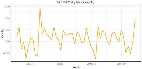
Figure 1.
Volatility of the international stock market.
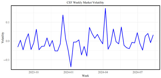
Figure 2.
Volatility of the Chinese carbon futures market.
The underlying reasons include the fact that the international stock market’s volatility is largely driven by macroeconomic factors, market sentiment, and global financial trends, particularly during times of significant policy changes or heightened economic uncertainty. On the other hand, being a developing market, the Chinese carbon futures market is more sensitive to policy adjustments, participant expectations, and speculative activities, resulting in more pronounced volatility.
Despite these differences, there is a degree of linkage between the two markets. For instance, during global economic fluctuations, the volatility of the international stock market can indirectly influence the Chinese carbon futures market. This connection is especially notable when global energy prices fluctuate, impacting operating and carbon emission costs for companies, thereby affecting the equilibrium between supply and demand in the Chinese carbon futures market. Consequently, during certain periods, the volatility of the Chinese carbon futures market and the international stock market can affect each other. Furthermore, changes in investor confidence in the international stock market may also transmit to the Chinese carbon futures market, leading to price fluctuations in the latter [38].
Figure 3 presents the volatility trends of the Chinese stock market. Compared with Figure 2, it is evident that the Chinese stock market generally exhibits moderate and stable volatility, with relatively lower amplitude and frequency of fluctuations than the Chinese carbon futures market. This stability suggests that, after years of development, the Chinese stock market has evolved into a relatively mature system with well-established trading structures and regulatory frameworks. However, in February 2024, a sharp spike in volatility is observed, reaching nearly 0.10. This anomaly likely reflects the combined effects of renewed concerns over real estate sector defaults, increased uncertainty in domestic regulatory policy, and heightened external risks stemming from shifting expectations of U.S. monetary policy. In contrast, the Chinese carbon futures market remains more sensitive to short-term policy changes and investor sentiment, highlighting its relatively early stage of market development.
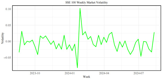
Figure 3.
Volatility of the Chinese stock market.
The volatility of the Chinese stock market is shaped largely by both domestic and international macroeconomic factors, company performance, and investor confidence, demonstrating strong resilience to risk. Meanwhile, the marked volatility in the Chinese carbon futures market reflects its still-developing market structure and complex participant composition, leaving it more vulnerable to external shocks such as policy changes and fluctuations in energy prices. This contrast highlights the need for increased regulatory oversight and policy support to guide the Chinese carbon futures market toward greater stability and maturity.
4.4. Mean Spillover Effect Analysis
The mean spillover effect primarily reflects the dynamic correlation both in stock market and the Chinese carbon futures market, as well as its variability across different periods. Figure 4 shows that the correlation of the international stock market with the Chinese carbon futures market undergoes significant fluctuations without a clear long-term trend. Notable periods include a strong positive correlation in October 2023 and January 2024, contrasted with significant negative correlations in November 2023 and March 2024. Overall, the correlation of the international stock market with the Chinese carbon futures market demonstrates pronounced short-term volatility, alternating between positive and negative values.
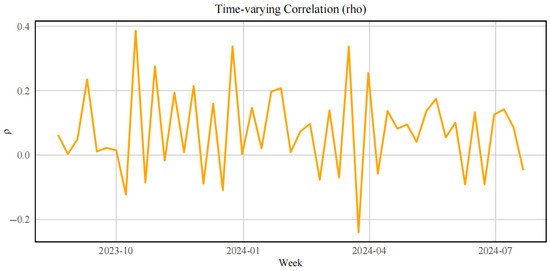
Figure 4.
Correlation between the international stock market and the Chinese carbon futures market.
Figure 5 presents the dynamic correlation trend of the Chinese stock market and the Chinese carbon futures market. This correlation also displays volatility and frequent changes, typically fluctuating between −0.2 and 0.2. During specific periods, such as January and April 2024, the correlation rises sharply, likely reflecting the impact of certain macroeconomic factors or policy adjustments. In contrast, during periods of heightened volatility, such as late 2023 and May 2024, the correlation shows a noticeable decline, indicating that distinct factors may be influencing the two markets at these times.
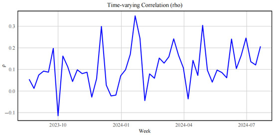
Figure 5.
Correlation between the Chinese stock market and the Chinese carbon futures market.
To further explore the changes in spillover strength under different market states, we divide the sample into different market regimes for comparative explanations based on the observed correlation fluctuations.
Phase I: August 2023 to November 2023.
During this relatively calm period, correlations in both panels remain close to zero, indicating weak spillover effects. This likely reflects stable macroeconomic conditions and limited cross-market shocks.
Phase II: December 2023 to January 2024.
A noticeable surge in correlation is observed—particularly in Figure 4, where international market correlations spike above 0.35, and in Figure 5, where correlations approach 0.3. These coincide with heightened global monetary policy shifts and China’s winter emission regulations, suggesting that both international and domestic factors jointly amplified cross-market volatility transmission during this period.
Phase III: February to April 2024.
Correlation levels decline sharply in Figure 4 and become volatile in Figure 5, reflecting divergent market responses. This period aligns with macro-policy recalibration and commodity price normalization. The correlation’s instability implies that spillover effects became more event-driven and less structurally stable.
Phase IV: May to August 2024.
Both figures show a gradual re-convergence toward moderate, positive correlations (~0.1–0.2), indicating the emergence of stable but lower-intensity spillover linkages. This may be due to adaptive investor behavior and policy digestion, as both markets returned to post-shock equilibrium.
Figure 4 illustrates the time-varying correlation between the international stock market and the Chinese carbon futures market. Notably, two sharp increases in correlation are observed around January and April 2024. These periods likely reflect the influence of significant macroeconomic and policy events. In January 2024, the People’s Bank of China announced a surprise reserve requirement ratio (RRR) cut, which boosted investor confidence and aligned sentiment across global and domestic markets. In April 2024, the announcement of new compliance rules and expanded emissions trading in China’s carbon market coincided with global discussions on climate finance, contributing to stronger co-movements.
Further analysis of Figure 4 reveals substantial volatility spillover effects in the Chinese stock market, international stock market, and Chinese carbon futures market. Variations in the international stock market often influence the Chinese carbon futures market and vice versa. For instance, during a global economic downturn, declining international equity prices typically indicate reduced economic activity and energy demand, which can lead to lower carbon futures prices. Conversely, during episodes of heightened global equity volatility, investors may view carbon futures as a relatively insulated or diversifying asset, increasing demand and driving short-term price movements. These dynamics underscore the interconnectedness of the three markets and emphasize the importance of cross-market monitoring and policy coordination.
Delving into the market mechanisms, when international companies face rising carbon emission costs, their production costs increase, potentially compressing profits and lowering stock prices. These companies may then seek to reduce their carbon allowances by increasing renewable energy usage, which decreases demand for carbon futures and leads to lower carbon prices. Conversely, if prices in the Chinese carbon futures market rise, companies may reduce the use of high-emission energy sources, thereby influencing price variations in energy market [39]. The observed correlation both in the international stock market and the Chinese carbon futures market provides a valuable opportunity for cross-market risk hedging. When volatility affects the international stock market, investors may balance their portfolios by counter-investing in the Chinese carbon futures market. This cross-market linkage effect is increasingly significant in the globalized financial market, providing a strategic basis for portfolio adjustments between these markets.
In addition, Figure 5 indicates that the connection within the Chinese stock market and the Chinese carbon futures market exhibits notable temporal heterogeneity. This volatility is influenced mainly by policy changes, market expectations, and energy price fluctuations. For example, when China implements new environmental policies or tightens carbon emission limits, the carbon market may see rising carbon prices, potentially leading to increased operating costs for companies and triggering volatility in the stock market. Conversely, when international energy prices decrease, companies may experience lower production and investment costs, easing price pressures in the carbon market and potentially boosting stock market performance. Understanding the dynamic relationship between these markets is crucial for investors seeking to optimize asset allocation and hedge against risk.
From a practical standpoint, the estimated spillover coefficient of −0.38 from the international stock market to the Chinese carbon futures market implies that a one-unit increase in global volatility may lead to a 38% reduction in volatility in the Chinese carbon market, assuming other factors remain constant. This suggests that carbon futures could serve as a partial hedge against global equity market fluctuations, offering diversification benefits to investors during international crises. Conversely, the positive spillover from the Chinese stock market (coefficient ≈ +0.32) highlights the close linkage between domestic financial sentiment and carbon pricing. This reflects a domestic transmission channel, through which macroeconomic conditions or regulatory signals influence the behavior of the carbon futures market.
In addition to the equity and carbon markets, we also identify some spillover interactions involving crude oil and gold. Crude oil occasionally exhibits transient shock transmission effects, especially during periods of commodity market volatility. On the other hand, gold appears to act more as a passive recipient of shocks, consistent with its role as a safe-haven asset. However, compared to the stronger and more persistent spillover dynamics within financial and carbon markets, these effects are relatively limited and less structurally robust. Therefore, our analysis prioritizes markets with clearer and more interpretable transmission channels.
Table 5 presents the estimated volatility spillover parameters among the international stock market (SP), Chinese stock market (SSE), and Chinese carbon futures market (CF), along with gold (GF) and crude oil (WTI). The results indicate several noteworthy transmission effects.
Table 5.
Estimation results of volatility spillover parameters.
Notably, the spillover effect from the international stock market (SP) to both the Chinese stock market (SSE: −0.30348) and the Chinese carbon futures market (CF: −0.37919) is negative. This suggests that heightened volatility in global equity markets tends to exert a dampening effect on China’s financial system. Specifically, increased uncertainty in the international market may lead to capital outflows, reduced risk appetite, and a more cautious stance by Chinese investors, ultimately weakening domestic market performance. In the case of the carbon futures market, which remains relatively sensitive to external sentiment and policy shifts, global shocks can reduce compliance demand expectations and suppress trading activity.
Conversely, the Chinese stock market shows a positive volatility spillover to the international stock market (SSE → SP: 0.50623), indicating that volatility in the Chinese market may also influence global investor sentiment, particularly during periods of heightened financial integration. Similarly, the spillover effect from SSE to CF (0.31995) implies that domestic equity market movements may stimulate trading activity or risk perception in the carbon futures segment, possibly due to overlapping institutional participation and macroeconomic linkages.
This complex spillover structure underscores the bidirectional nature of volatility transmission across asset classes and regions. It also reflects the increasing integration of China’s financial markets into the global system, where local shocks can have international ramifications and vice versa. Understanding these interactions is essential for policymakers and investors seeking to manage risk in an interconnected financial environment.
4.5. Model Verification
Trace plots are widely used diagnostic tools in Bayesian estimation to assess whether an MCMC chain has achieved convergence. A well-converged trace plot will exhibit random fluctuations of the parameters around their values within the posterior distribution, with no evident upward or downward trends. This stable, trendless random pattern indicates that the MCMC sampling process has moved past the impact of the initial values and has reached a steady state, suggesting reliable parameter estimates within the posterior distribution.
Figure 6, Figure 7, Figure 8 and Figure 9 display trace plots and time series iteration graphs that indicate relatively stable random fluctuations, suggesting that parameter sampling within the posterior distribution has reached convergence. The sampling process appears stable, with no noticeable trend shifts. Specifically, Figure 7 and Figure 9 illustrate parameter fluctuations in the international stock market and the Chinese carbon futures market, respectively. The parameters in these figures fluctuate within a narrow range, with no significant trend changes observed over the analyzed period. While volatility levels differ between the two markets, both demonstrate a degree of stability, revealing insights into the dynamic characteristics and fluctuations in the international stock market and the Chinese carbon futures market over time [40].
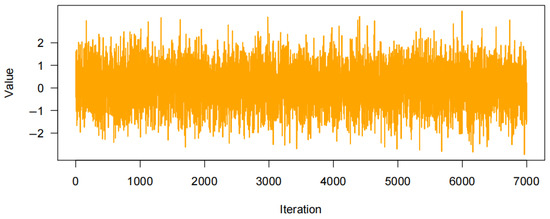
Figure 6.
Trace plot of .
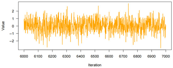
Figure 7.
Time series iteration results of .
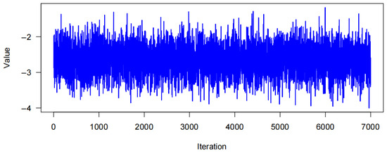
Figure 8.
Trace plot of .
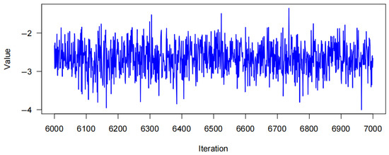
Figure 9.
Time series iteration results of .
Figure 6 and Figure 8 further confirm that parameters for the international stock market and the Chinese carbon futures market have achieved convergence in the MCMC sampling, as the trace plots exhibit trendless random fluctuations. This indicates that the sampling chains have moved beyond initial value influences and thoroughly explored the posterior distribution of the parameters.
The Chinese carbon futures market and the Chinese stock market exhibit similar convergence characteristics to those both in the international stock market and the Chinese carbon futures market. Due to space limitations, specific trace plots for these are not included in the text.
4.6. Model Convergence Analysis
Model convergence analysis assesses whether the model parameters or the loss function value stabilize as iterations increase, indicating that the model has reached an optimal result. The Gelman–Rubin diagnostic is commonly used for this purpose, evaluating convergence by examining multiple independent chains. A value of the potential scale reduction factor (PSRF) close to 1 suggests that the chains have converged. The essence of this analysis is to determine if the model parameters have reached a steady state within the posterior distribution. Figure 10 presents the results of this model convergence analysis, highlighting the stability and convergence of the model parameters.
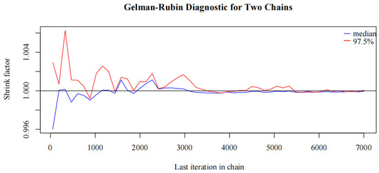
Figure 10.
Gelman–Rubin diagnostic.
Figure 10 illustrates the Gelman–Rubin diagnostic results of the two MCMC chains. Detailed analysis reveals that with an increasing number of iterations of the shrinkage factor, its value gradually approaches 1, stabilizing after 2000 iterations. This trend indicates that the two independent chains have converged, the posterior distribution of the model parameters has reached stability, confirming both model convergence and the reliability of the parameter estimates. The initial fluctuations represent the chains’ adaptation phase, while the stable phase reflects effective mixing of the chains. Thus, it can be concluded that the model has adequately converged, ensuring that the sample used for subsequent analysis carries statistical significance.
4.7. Robustness Check: Subsample Analysis
To verify the robustness of the baseline results, we conduct a subsample analysis by dividing the full sample into two equal-length periods. The model is re-estimated using each subsample separately, and the posterior densities of key parameters are compared.
Figure 11 presents the posterior densities of (3,1), which captures the spillover effect from the S&P 500 index to the carbon futures market. Both distributions center around positive values, with substantial overlap, indicating that the direction and significance of spillovers remain consistent across different periods.
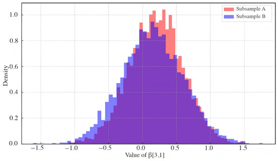
Figure 11.
Posterior densities of (3,1) in subsample A (red) and subsample B (blue).
Figure 12 displays the posterior densities of (3), the volatility persistence parameter of the carbon futures market. The distributions are heavily concentrated near 0.9–1.0 in both subsamples, suggesting stable and persistent volatility behavior.
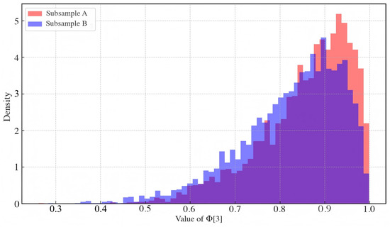
Figure 12.
Posterior densities of (3) in subsample A (red) and subsample B (blue).
Together, these results demonstrate that the dynamic spillover structure and volatility dynamics identified by the DGC-t-MSV-BN model are robust to temporal segmentation.
4.8. Forecast Evaluation
To assess the out-of-sample predictive capability of the DGC-t-MSV-BN model, we conduct rolling one-step-ahead forecasts for five core financial series: the international stock market (SP), Chinese stock market (SSE), Chinese carbon futures market (CEF), gold (GOLD), and crude oil (WTI). The forecasts are generated using a rolling expanding-window framework based on an autoregressive specification, with the first 40 observations used for initialization and the remaining 12 observations reserved for testing.
At each step, we re-estimate the model and produce a one-week-ahead forecast. Forecast accuracy is assessed using two standard metrics: the Root Mean Squared Forecast Error (RMSFE) and the Mean Absolute Error (MAE). Table 6 summarizes the predictive accuracy of the model for each series.
Table 6.
Out-of-sample forecast accuracy for each market variable.
The results reveal notable differences in predictive performance across asset classes. The international stock market (SP) exhibits the lowest prediction errors, indicating relatively strong model performance in capturing stable and mature market dynamics. GF and SSE also show moderate forecast accuracy, suggesting the model effectively identifies their short-term trends. In contrast, the Chinese carbon futures (CEF) and crude oil (WTI) markets produce higher prediction errors, reflecting their inherently higher volatility and greater sensitivity to external shocks and structural policy changes.
Although forecasting is not the primary focus of this study, these results demonstrate that the proposed model can deliver reasonably reliable short-term forecasts for various asset types. The performance discrepancy also highlights the distinct volatility characteristics and structural features of each market. These findings support the robustness of the DGC-t-MSV-BN model while also identifying areas for potential model enhancement or hybridization for high-volatility assets.
4.9. Sensitivity Analysis
To evaluate the robustness of the model estimates to prior specification and parameter assumptions, we conduct a qualitative sensitivity analysis focusing on the key structural components of the DGC-t-MSV-BN model. Specifically, we examine the impact of varying the prior distributions for the volatility persistence parameter () and the degrees of freedom () of the Student-t innovations.
For , the baseline beta (20, 1.5) prior is replaced with more diffuse alternatives such as beta (5, 1.5) and beta (10, 2), which assume lower prior belief in high persistence. For the degrees of freedom , we substitute the original exponential (0.1) prior with heavier-tailed and lighter-tailed alternatives, including exponential (0.2) and gamma (2, 0.1). While these modifications affect the dispersion and tail behavior of the posterior distributions, the key empirical findings—such as the direction and magnitude of volatility spillovers from the international stock market (SP) to the Chinese carbon futures market (CEF)—remain qualitatively stable.
Additionally, we observe that the dynamic network structure inferred from the Bayesian graphical layer is not materially affected by moderate prior changes. The number of active edges and dominant transmission pathways remain largely consistent across prior settings.
In summary, the DGC-t-MSV-BN model demonstrates robustness to reasonable variations in prior assumptions. The stability of key spillover parameters and the network topology under alternative specifications reinforces the credibility of the model’s inference and its suitability for capturing dynamic volatility interdependence.
4.10. Consideration of Structural Market Changes
While this study primarily focuses on modeling dynamic volatility spillovers across markets, we acknowledge that structural breaks or regime shifts—such as major policy reforms, the introduction of carbon trading mechanisms, or abrupt shifts in investor behavior—can influence the transmission of volatility across financial systems.
Although the DGC-t-MSV-BN framework does not explicitly model structural breaks, two steps are taken to mitigate their potential effects. First, the use of a time-varying stochastic volatility model with Bayesian graphical learning allows for flexible adaptation to evolving inter-market dependencies without imposing fixed relationships. Second, the sample period captures a particularly active phase of financial reform and climate policy adjustment in China, providing a relevant empirical context for assessing short-term regime-sensitive behavior.
Future extensions may incorporate regime-switching components or structural break tests to more explicitly identify the timing and impact of institutional or regulatory shifts on volatility propagation patterns.
4.11. Bayesian Network Visualization
The Bayesian network in this paper is constructed using GeNIe, assuming consistent initial probabilities for volatility spillover across markets. Based on the notable volatility spillover parameters in Table 4, relationships among markets, including the international stock market, were identified, as depicted in Figure 13. This figure illustrates the initial state diagram of the Bayesian network based on model estimates, highlighting fundamental inter-market relationships without external shocks.
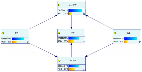
Figure 13.
Initial state diagram of the Bayesian network.
Figure 13, Figure 14 and Figure 15 reveal that volatility spillover effects among the Chinese carbon futures market, international crude oil and gold futures markets are relatively low. This suggests limited mutual influence among these markets under typical conditions, particularly the low volatility correlation between the Chinese carbon futures market and international crude oil and gold futures markets. Figure 13 provides an intuitive overview of the basic spillover effects among markets, establishing a foundation for further analysis of spillover dynamics during market crises.
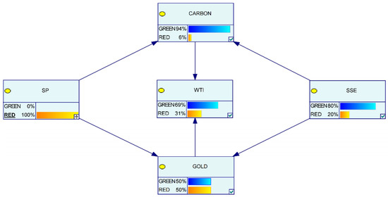
Figure 14.
Final state diagram of the Bayesian network during a severe crisis in the international stock market.
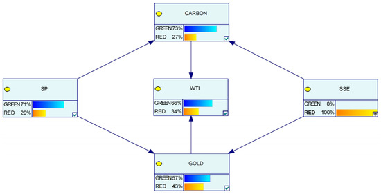
Figure 15.
Final state diagram of the Bayesian network during a severe crisis in the Chinese stock market.
Figure 14 and Figure 15 examine the spillover effects during severe crises in the international and Chinese stock markets. In Figure 14, a crisis in the international stock market corresponds with a significant decrease in volatility in the Chinese carbon futures market, suggesting minimal spillover effects from international crude oil and gold futures markets and highlighting a certain safe-haven function of the Chinese carbon futures market.
Conversely, Figure 15 shows that when a crisis occurs within the Chinese stock market this leads to a marked rise in volatility within the Chinese carbon futures market. Although its connection to international commodity markets remains weak, the internal volatility escalates, underscoring the high volatility and immaturity characteristic of the Chinese carbon futures market as an emerging market. Nonetheless, as market mechanisms strengthen and policy support grows, improvements in liquidity and transparency are expected, enhancing the influence and role of the Chinese carbon futures market in the global financial landscape.
In conclusion, the impact of a crisis in the international stock market on the Chinese carbon futures market appears relatively minor, suggesting either a low correlation between the two or a safe-haven function within the Chinese carbon futures market. In contrast, a crisis in the Chinese stock market has a pronounced influence on the Chinese carbon futures market, indicating a stronger correlation or heightened sensitivity of the Chinese carbon futures market to events in the Asian market. Additionally, being a developing market, the Chinese carbon futures market currently displays high volatility and certain signs of immaturity. However, with ongoing improvements in market mechanisms and increased policy support, the Chinese carbon futures market is developing rapidly and gradually taking on a more influential role in the global market landscape.
5. Concluding Remarks
5.1. Conclusions
This paper constructs an enhanced Dynamic Conditional Correlation Stochastic Volatility (DGC-t-MSV) model. It combines this with a Bayesian network (BN) to create the DGC-t-MSV-BN model. The empirical study yields the following main conclusions:
(1) There are substantial volatility spillover effects among Chinese and international stock markets, as well as the Chinese carbon futures market, indicating close connections within the global financial landscape. The volatility in Chinese and international stock markets impacts the Chinese carbon futures market, and fluctuations in carbon emission costs can affect company stock prices. This connection presents opportunities for strategic adjustments and cross-market risk hedging between stock and carbon futures markets in a globalized setting. While a crisis in the international stock market has a relatively minor influence on the Chinese carbon futures market, suggesting a safe-haven function or weaker correlation, a crisis in the Chinese stock market leads to significant fluctuations in the Chinese carbon futures market, highlighting a strong linkage and sensitivity within the local financial environment.
(2) The spillover effect from the international stock market to the Chinese carbon futures market is negative, meaning that international market volatility negatively impacts the Chinese carbon market, potentially reducing activity or suppressing price changes. Conversely, the spillover from the Chinese stock market to the Chinese carbon market is positive, suggesting that fluctuations in the Chinese stock market can stimulate carbon market activity. This complex spillover pattern underscores the high interdependence among the Chinese, international, and carbon markets, particularly during global economic events. Effective strategies should thus fully consider the interconnectedness and risk transmission mechanisms among these markets.
(3) The connection between the Chinese carbon futures market and international gold and crude oil futures markets is weak, with limited volatility spillover effects. While the Chinese carbon futures market currently displays high volatility and lower market maturity, improvements in liquidity and transparency are expected as carbon emissions control policies advance and market mechanisms mature. The Chinese carbon futures market is poised to become an important platform for global carbon pricing, contributing more significantly to climate change mitigation and sustainable development.
5.2. Limitations
This study presents a dynamic analysis of volatility spillovers between the Chinese stock and carbon futures markets using weekly frequency data. However, the current scope remains limited to a single national market and does not capture broader regional or international financial linkages. Moreover, while the DGC-t-MSV-BN model effectively models structural and volatility-based transmission channels, it does not yet account for critical drivers such as market liquidity, investor sentiment, or regulatory interventions. Liquidity conditions—measured by variables like turnover, bid-ask spreads, or illiquidity ratios—may significantly influence spillover dynamics, particularly under market stress, but were not included due to data constraints. Additionally, behavioral factors such as investor sentiment, herding, or risk aversion may amplify volatility spillovers, especially during crises, yet are not explicitly incorporated in the model. Lastly, the potential impact of regulatory changes—such as adjustments to China’s carbon trading scheme or international ESG policies—remains unaddressed. These omissions represent important avenues for future research to improve the robustness, interpretability, and global relevance of the analysis.
5.3. Originality and Value
This paper pioneers the integration of a t-distributed multivariate stochastic volatility model with a Bayesian network for spillover analysis, providing a novel tool for identifying both directional and time-varying relationships across multiple asset markets. It uniquely applies this hybrid method to the intersection of China’s carbon futures market, domestic equities, and global financial systems—an area still underexplored in the existing literature.
5.4. Theoretical and Practical Contributions
This study makes both theoretical and practical contributions. Theoretically, it enhances the modeling of volatility transmission by incorporating heavy-tailed distributions and directed dependency structures through the DGC-t-MSV-BN framework. Practically, the findings offer valuable implications for both institutional investors and policymakers. The identified asymmetric volatility spillovers suggest that carbon futures can serve as effective risk management tools, particularly during periods of international financial turbulence. For institutional investors and risk managers, understanding these spillover dynamics enables the development of more robust cross-market hedging strategies and informed asset allocation during market shocks. For regulators, the observed sensitivity of China’s carbon market to domestic equity movements underscores the importance of coordinated oversight between carbon pricing mechanisms and financial markets. As China continues to expand its carbon trading system, recognizing these interlinkages is critical to enhancing market resilience, improving policy effectiveness, and supporting the holistic supervision of emerging green finance systems.
5.5. Future Research Directions
Although this study primarily focuses on volatility spillovers between the Chinese stock market and the carbon futures market, the findings offer broader implications for other asset classes and financial systems. The proposed modeling framework can be extended to analyze spillover effects in commodities, foreign exchange markets, and emerging economies, enabling cross-market comparisons under different market structures, liquidity levels, and economic conditions. Future research could further explore whether similar spillover patterns hold across diverse regions, particularly by incorporating developed versus emerging markets. In addition, examining the role of market-specific factors—such as regulatory environments and policy shifts—may help uncover how institutional differences shape volatility transmission, thereby offering a more nuanced understanding of global financial interconnectedness and supporting more effective risk management strategies.
Author Contributions
J.W.: Conceptualization and methodology. T.M.: writing—original draft preparation and analysis. L.W.: calculation and supervision. J.W. and L.W. contributed equally to this work. They are co-first authors. All authors have read and agreed to the published version of the manuscript.
Funding
This research is supported by the Later-stage Funding Project of the National Social Science Fund (24FGLB100); Major Strategic and Policy-Oriented Bidding Projects in Jiangsu Province’s Educational Science Planning (JS/2024/ZD0104-01849).
Data Availability Statement
The original contributions presented in this study are included in the article. Further inquiries can be directed to the corresponding author.
Conflicts of Interest
The authors declare no conflicts of interest.
References
- Yang, W.R.; Chuang, M.C. Do investors herd in a volatile market? Evidence of dynamic herding in Taiwan, China, and US stock markets. Financ. Res. Lett. 2023, 52, 103364. [Google Scholar] [CrossRef]
- Elsayed, A.H.; Asutay, M.; ElAlaoui, A.O.; Bin Jusoh, H. Volatility spillover across spot and futures markets: Evidence from dual financial system. Res. Int. Bus. Financ. 2024, 71, 102473. [Google Scholar] [CrossRef]
- Lin, B.; Lan, T. The time-varying volatility spillover effects between China’s coal and metal market. J. Futures Mark. 2024, 44, 699–719. [Google Scholar] [CrossRef]
- Ren, X.; Xiao, S.; Zhang, W.; Sun, X. Tail risk spillover of commodity futures markets. Account. Financ. 2025, 65, 109–141. [Google Scholar] [CrossRef]
- Phan, I.; Luo, X.; Adelopo, I. Global spillover persistence and market resilience during uncertainty. J. Cap. Mark. Stud. 2025. [Google Scholar] [CrossRef]
- Hou, Y.; Li, W.; Wu, D.; Zang, Y.; Quach, L. The spillover effect of US monetary policy on the international financial market: Evidence from network analysis. J. Manag. Sci. Eng. 2025, 10, 111–125. [Google Scholar] [CrossRef]
- Iqbal, N.; Bouri, E.; Liu, G.; Kumar, A. Volatility spillovers during normal and high volatility states and their driving factors: A cross-country and cross-asset analysis. Int. J. Financ. Econ. 2024, 29, 975–995. [Google Scholar] [CrossRef]
- Cheng, Z.; Li, M.; Cui, R.; Wei, Y.; Wang, S.; Hong, Y. The impact of COVID-19 on global financial markets: A multiscale volatility spillover analysis. Int. Rev. Financ. Anal. 2024, 95, 103454. [Google Scholar] [CrossRef]
- Wang, L.; Wang, Y.; Wang, J.; Yu, L. Forecasting Nonlinear Green Bond Yields in China: Deep Learning for Improved Accuracy and Policy Awareness. Financ. Res. Lett. 2025, 85, 107889. [Google Scholar] [CrossRef]
- Chen, T.; Zheng, X.; Wang, L. Systemic risk among Chinese oil and petrochemical firms based on dynamic tail risk spillover networks. N. Am. J. Econ. Financ. 2025, 77, 102404. [Google Scholar] [CrossRef]
- Wang, Z.; Dong, Z. Volatility spillover effects among geopolitical risks and international and Chinese crude oil markets——A study utilizing time-varying networks. Resour. Policy 2024, 96, 105225. [Google Scholar] [CrossRef]
- Su, T.; Lin, B. Reassessing the information transmission and pricing influence of Shanghai crude oil futures: A time-varying perspective. Energy Econ. 2024, 140, 107977. [Google Scholar] [CrossRef]
- Naeem, M.A.; Qureshi, F.; Farid, S.; Tiwari, A.K.; Elheddad, M. Time-frequency information transmission among financial markets: Evidence from implied volatility. Ann. Oper. Res. 2024, 334, 701–729. [Google Scholar] [CrossRef]
- Yi, D.; Lin, S.; Yang, J. Global Climate Risk Perception and Its Dynamic Impact on the Clean Energy Market: New Evidence from Contemporaneous and Lagged R2 Decomposition Connectivity Approaches. Sustainability 2025, 17, 3596. [Google Scholar] [CrossRef]
- Zhao, X.; Wang, X.; Golay, M.W. Bayesian network–based fault diagnostic system for nuclear power plant assets. Nucl. Technol. 2023, 209, 401–418. [Google Scholar] [CrossRef]
- Zhou, W.; Chen, Y.; Chen, J. Dynamic volatility spillover and market emergency: Matching and forecasting. N. Am. J. Econ. Financ. 2024, 71, 102110. [Google Scholar] [CrossRef]
- Arfaoui, N.; Roubaud, D.; Naeem, M.A. Energy transition metals, clean and dirty energy markets: A quantile-on-quantile risk transmission analysis of market dynamics. Energy Econ. 2025, 143, 108250. [Google Scholar] [CrossRef]
- Lu, C.; Liu, L.; Yu, F.; Li, J.; Zheng, G. Mapping Extent of Spillover Channels in Monetary Space: Study of Multidimensional Spatial Effects of US Dollar Liquidity. Int. J. Financ. Stud. 2025, 13, 72. [Google Scholar] [CrossRef]
- Bollerslev, T.; Engle, R.F.; Nelson, D.B. ARCH models. In Handbook of Econometrics; Elsevier: Amsterdam, The Netherlands, 1994; Volume 4, pp. 2959–3038. [Google Scholar] [CrossRef]
- Taylor, S.J. Modeling stochastic volatility: A review and comparative study. Math. Financ. 1994, 4, 183–204. [Google Scholar] [CrossRef]
- Pelletier, D.; Wei, W. A stochastic price duration model for estimating high-frequency volatility. J. Financ. Econom. 2024, 22, 1372–1396. [Google Scholar] [CrossRef]
- Habib, S.; Habib, M.; Batool, S. Cross-Market Volatility Dynamics Among Crude Oil and South Asian Emerging Markets During the COVID-19 Pandemic. Int. J. Manag. Res. Emerg. Sci. 2024, 14. [Google Scholar] [CrossRef]
- Cheung, K.T. Application and Empirical Analysis of Random Volatility Model in Financial Markets. Highlights Bus. Econ. Manag. 2024, 41, 620–624. [Google Scholar] [CrossRef]
- Chen, W.; Chen, Z.; Luo, Q. Predicting volatility in China’s clean energy sector: Advantages of the carbon transition risk. Financ. Res. Lett. 2025, 72, 106534. [Google Scholar] [CrossRef]
- Engle, R. Dynamic Conditional Correlation: A Simple Class of Multivariate Generalized Autoregressive Conditional Heteroskedasticity Models. J. Bus. Econ. Stat. 2002, 20, 339–350. [Google Scholar] [CrossRef]
- Hou, J.; Wang, P.; Borjigin, S. Dependence and risk spillover effects between clean energy stocks and related assets—An empirical study based on asymmetric W-TVP-VAR model. Appl. Econ. 2025, 1–32. [Google Scholar] [CrossRef]
- Soltani, H.; Abbes, M.B. Regime-specific spillover effects between financial stress, GCC stock markets, Brent crude oil, and the gold market. J. Knowl. Econ. 2025, 16, 8840–8866. [Google Scholar] [CrossRef]
- He, Z.; Liu, Z.; Zhang, C.; Zhao, Y. How do carbon pricing spillover effects impact green asset price volatility? An empirical study based on the TVP-VAR-DY model. Econ. Anal. Policy 2025, 85, 2162–2179. [Google Scholar] [CrossRef]
- Tripathy, P.; Brahmi, M.; Pallayil, B.; Mishra, B.R. Mediating Effects of Foreign Direct Investment Inflows on Carbon Dioxide Emissions. Economies 2025, 13, 18. [Google Scholar] [CrossRef]
- Chan, L.S.H.; Chu, A.M.Y.; So, M.K.P. A moving-window bayesian network model for assessing systemic risk in financial markets. PLoS ONE 2023, 18, e0279888. [Google Scholar] [CrossRef]
- Ji, Y.; Xu, Z.; Zhao, C.; Chen, K.; Du, Y. Accelerated Testing and Evaluation for Black-Box Autonomous Driving Systems via Adaptive Markov Chain Monte Carlo. IEEE Trans. Intell. Transp. Syst. 2025, 26, 6463–6476. [Google Scholar] [CrossRef]
- Laal, N.; Taylor, S.R.; van Haasteren, R.; Lamb, W.G.; Siemens, X. Solving the PTA data analysis problem with a global Gibbs scheme. Phys. Rev. D 2025, 111, 063067. [Google Scholar] [CrossRef]
- Geman, S.; Geman, D. Stochastic relaxation, Gibbs distributions, and the Bayesian restoration of images. IEEE Trans. Pattern Anal. Mach. Intell. 1984, PAMI-6, 721–741. [Google Scholar] [CrossRef]
- Robert, C.P.; Casella, G. Monte Carlo Statistical Methods. In Springer Texts in Statistics; Springer: New York, NY, USA, 2004. [Google Scholar] [CrossRef]
- Stefanou, A.D.; Zianni, X. Physics mechanisms underlying the optimization of coherent heat transfer across width-modulated nanowaveguides with calculations and machine learning. J. Phys. Condens. Matter 2024, 36, 245301. [Google Scholar] [CrossRef]
- Al-Raeei, M. Morse potential specific bond volume: A simple formula with applications to dimers and soft–hard slab slider. J. Phys. Condens. Matter 2022, 34, 284001. [Google Scholar] [CrossRef]
- Hong, S. Solving inference problems of Bayesian networks by probabilistic computing. AIP Adv. 2023, 13, 075226. [Google Scholar] [CrossRef]
- Liu, J.B.; Yuan, X.Y.; Lee, C.C. Prediction of carbon emissions in China’s construction industry using an improved grey prediction model. Sci. Total Environ. 2024, 938, 173351. [Google Scholar] [CrossRef]
- Liu, J.B.; Liu, B.R.; Lee, C.C. Efficiency evaluation of China’s transportation system considering carbon emissions: Evidence from big data analytics methods. Sci. Total Environ. 2024, 922, 171031. [Google Scholar] [CrossRef]
- Wang, J.; Zeng, R.; Wang, L. Volatility Spillover Between the Carbon Market and Traditional Energy Market Using the DGC-t-MSV Model. Mathematics 2024, 12, 3789. [Google Scholar] [CrossRef]
Disclaimer/Publisher’s Note: The statements, opinions and data contained in all publications are solely those of the individual author(s) and contributor(s) and not of MDPI and/or the editor(s). MDPI and/or the editor(s) disclaim responsibility for any injury to people or property resulting from any ideas, methods, instructions or products referred to in the content. |
© 2025 by the authors. Licensee MDPI, Basel, Switzerland. This article is an open access article distributed under the terms and conditions of the Creative Commons Attribution (CC BY) license (https://creativecommons.org/licenses/by/4.0/).