Abstract
This study evaluates hierarchical clustering methodologies to identify patterns associated with timeout requests for EuroLeague basketball games. Using play-by-play data from 3743 games spanning the 2008–2023 seasons (over 1.9 million instances), we applied Principal Component Analysis to reduce dimensionality and tested multiple agglomerative and divisive clustering techniques (e.g., Ward and DIANA) with different distance metrics (Euclidean, Manhattan, and Minkowski). Clustering quality was assessed using internal validation indices such as Silhouette, Dunn, Calinski–Harabasz, Davies–Bouldin, and Gap statistics. The results show that Ward.D and Ward.D2 methods using Euclidean distance generate well-balanced and clearly defined clusters. Two clusters offer the best overall quality, while four clusters allow for meaningful segmentation of game situations. The analysis revealed that teams that did not request timeouts often exhibited better scoring efficiency, particularly in the advanced game phases. These findings offer data-driven insights into timeout dynamics and contribute to strategic decision-making in professional basketball.
MSC:
62H30; 68T10; 91A80
1. Introduction
Basketball is a sport where coaching decisions can significantly impact game outcomes. Among these decisions, timeouts are a limited but powerful strategic tool used to influence momentum, adjust tactics, and manage player fatigue. Traditionally, such decisions were guided by intuition and subjective experience [1,2] and were often supported by video analysis [3]. However, the rise of data analytics in sports has promoted a more evidence-based approach to decision-making [4].
As coaching staff and executives increasingly recognise the competitive advantage of data-informed strategies [5], interest has grown in analysing how specific in-game decisions—such as calling timeouts—relate to broader game dynamics. The EuroLeague, Europe’s top-tier basketball competition, provides a compelling context for this analysis because of its slower pace, greater strategic complexity, and high level of coaching expertise involved [6,7,8,9].
Despite the growing field of basketball analytics, research on timeout usage in FIBA competitions is still limited. Most existing studies focus on the NBA [10,11,12]. Prior work has shown that timeouts can interrupt scoring runs, support tactical changes, or address psychological and physical demands [13,14,15,16]. However, factors such as score margin, game timing, and sequence of events influence when and why timeouts are used.
This study addresses this gap by analysing the context in which timeouts are requested in EuroLeague basketball. The objective of the proposed method is to evaluate the effectiveness of different hierarchical clustering techniques—applying various linkage methods and distance metrics—to identify meaningful patterns in the timing and characteristics of timeout requests. The findings support strategic decision-making in professional basketball and contribute to the broader field of sports analytics.
Therefore, the present study seeks to answer the following question: Can hierarchical clustering methodologies identify meaningful patterns in the timing and contextual characteristics of timeout requests in EuroLeague basketball games?
2. Related Work
In recent years, sports analytics has increasingly incorporated advanced unsupervised learning techniques, particularly clustering methods, to extract patterns from complex in-game data. In basketball, clustering has been applied to classify playing styles, segment game phases, and identify tactical patterns [11,17].
Ref. [18] applied clustering techniques to model the influence of players’ offensive roles on overall team performance in the Chinese Basketball Association (CBA). Using a combination of spatial features and play-type frequency data, they employed unsupervised algorithms to identify distinct offensive archetypes. Their findings linked team success to the distribution and synergy of these roles within lineups, reinforcing the value of clustering for tactical evaluation and performance optimisation.
Ref. [19] employed both hierarchical and k-means clustering to group players by shooting style and offensive role, offering a framework to assess lineup composition and tactical functionality. Though centered on the Japanese B.League, their work demonstrates the effectiveness of clustering for mapping offensive structure and player interactions.
Further expanding this line of research, Ref. [20] proposed a dual-clustering approach combining the clustering of individual shooting styles with the clustering of shots themselves using optical tracking data. By applying hierarchical clustering with Wasserstein and Gower distances, they generated interpretable shooting profiles that captured not only location but also shot creation patterns, offering a refined tool for performance analysis.
Ref. [21] conducted a cluster analysis on players in the Turkish Basketball Super League, applying k-means to performance statistics to uncover role diversity beyond traditional positional labels. Their work demonstrated the utility of clustering in refining player classification for tactical planning and roster development.
Most existing clustering studies in basketball have focused on NBA data, capitalising on its availability and granularity. Ref. [22] applied Bayesian nonparametric tensor clustering to NBA shot charts to reveal heterogeneous player shooting patterns. Similarly, Ref. [23] used matrix clustering to estimate latent spatial behaviours, while Ref. [24] combined PCA and clustering to link player attributes with performance and salary structures. Ref. [25] used optimal transport embeddings to compare team styles in collective sports, including the NBA. These works underscore the NBA-centric emphasis in the clustering literature and highlight the methodological novelty of applying similar techniques to FIBA contexts like the EuroLeague.
A growing number of studies have begun to apply clustering techniques in FIBA basketball, particularly in European competitions. Ref. [26] analysed EuroLeague and national league data from 2014 to 2016, identifying performance profiles through two-step clustering and discriminant analysis. Ref. [27] focused on the FIBA Basketball World Cup 2019, clustering team lineups based on anthropometric profiles and linking them to on-court performance metrics. These contributions support the relevance of clustering for modeling strategic configurations in FIBA basketball.
Despite increasing interest in basketball analytics, research focused specifically on timeout usage remains scarce. Ref. [28] evaluated the causal effect of timeouts on halting opponent scoring runs in the NBA, offering empirical support for timeout timing as a tactical intervention. In the EuroLeague, Ref. [29] examined timeout effectiveness using regression models across different game phases. However, no published studies have used clustering to segment or interpret timeout patterns. The present work addresses this gap by applying hierarchical clustering to identify structural dynamics in timeout requests, contributing a novel exploratory framework to the study of coaching decisions in professional basketball.
3. Materials and Methods
3.1. Clustering Techniques
In this study, we applied a range of hierarchical clustering methods to analyse timeout request patterns in EuroLeague Basketball games using detailed play-by-play data. The hierarchical clustering method was chosen over the partitioning and density-based methods due to its flexibility, interpretability, and ability to explore groupings at multiple levels without requiring a predefined number of clusters [30,31,32]. This is particularly relevant for exploratory analysis in sports contexts where the underlying structure of events may not be known in advance.
We evaluated both agglomerative and divisive approaches. The agglomerative methods included single linkage [33], complete linkage [34], average linkage [35], Ward.D linkage [36], Ward.D2 linkage [37], median linkage [38], centroid linkage [35], and McQuitty linkage [39] (Table 1). In addition, the DIANA [40] algorithm was applied as a representative divisive method. These techniques were selected to capture a diverse range of clustering behaviours, ranging from methods that prioritise compactness to those that emphasise cluster separation.

Table 1.
Summary of hierarchical clustering methods evaluated in this study.
Table 1 provides a concise comparison of the theoretical and practical characteristics of each hierarchical clustering method, which helps contextualise their performance in later stages of the analysis.
3.2. Distance Metrics and Validation Indices
To examine the impact of distance sensitivity on clustering quality, we applied each method using three different distance metrics [58]: Euclidean distance, Manhattan distance, and Minkowski:
- The Euclidean distance measures the actual distance between two points in Euclidean space. The length of the line segment connecting two points in this space can be calculated using the Pythagorean Theorem. That is, given two points P = (p1, …, pn) and Q = (q1, …, qn), in n-dimensional space, the Euclidean distance de between P and Q is defined as:
- The Manhattan distance, also known as the L1 distance or taxicab distance, is a metric that calculates the distance between two points in a grid-based space based on a rectilinear path parallel to the axes. It is defined as the sum of absolute differences in their coordinates. That is, given two points, P = (p1, …, pn) and Q = (q1, …, qn), in n-dimensional space, the Manhattan distance dma between P and Q is defined as:This distance, instead of measuring the most direct path as the Euclidean distance, measures only paths that move along the axes at right angles. This distance is particularly useful when you want the metric to be more robust to extreme variations in any direction.
- Minkowski distance is a generalisation of Euclidean and Manhattan distances and is used to measure the distance between two points in an n-dimensional normed space. Given two points, P = (p1, …, pn) and Q = (q1, …, qn), in n-dimensional space, the Minkowski distance dmi between P and Q is defined as:where r is a positive real number that determines the generality of the distance metric. When r takes the value 1, this distance is equivalent to the Manhattan distance, and to the Euclidean distance when r takes the value 2.
This distance is very useful because the option to select the parameter r allows for adjusting the sensitivity to differences across various dimensions of the data. For this study, the parameter r = 3 will be considered.
Each clustering solution was evaluated using the following set of internal validation indices:
- Cophenetic Correlation Coefficient [59], to evaluate how well the dendrogram represents the original distances. Values close to 1 indicate that the dendrogram well represents the actual pairwise distances.
- Elbow Method [60], to identify the optimal number of clusters based on locating the ‘elbow’ point where the rate of decrease in within-cluster sum of squares slows significantly.
- Silhouette Index [61], to assess cohesion within and separation between clusters. Values close to 1 indicate well-separated clusters; negative values suggest poor clustering.
- Gap Statistic [62], comparing the observed clustering structure to that expected under a null model. Higher gap values suggest stronger evidence for the number of clusters.
- Calinski–Harabasz Index [63], to measure the ratio of between-cluster to within-cluster dispersion. Higher values indicate better-defined and compact clusters.
- Dunn Index [64], which favors compact and well-separated clusters. Higher values indicate more distinct and compact clusters.
- Davies–Bouldin Index [65], where lower values indicate better clustering structure. Lower values indicate better clustering quality (less overlap).
This combination of methods and validation metrics allowed us to comprehensively assess clustering quality and robustness for interpreting timeout dynamics in professional basketball.
3.3. EuroLeague Play-by-Play Dataset
The dataset was compiled from publicly accessible play-by-play data provided by the EuroLeague Game Center (https://www.euroleaguebasketball.net/en/euroleague/game-center/, accessed on 3 August 2023).
For this purpose, play-by-play data (1,919,273 instances) from all EuroLeague games played across 15 seasons, spanning 2008–2009 to 2022–2023, were selected. As noted in the introduction, during this period, previous FIBA regulations allowed teams to request three timeouts during the second half of games (quarters 3 and 4). This dataset encompasses a total of 3743 games, from which the traditional box score information of both teams in each game was extracted: minutes played, points scored, one-point, two-point, and three-point attempts and conversions, assists, defensive and offensive rebounds, turnovers, blocks, and personal fouls committed. In addition to contextual variables, 21 quantitative variables on the statistical summaries of each action coded in the play-by-play were analysed.
The variable under study is “timeout request”, typically coded in EuroLeague play-by-play data with the following values: (i) “Time Out (1),” indicating that the timeout is the first requested during that specific time period (first half, second half, or overtime); (ii) “Time Out (2),” for the second timeout requested in either the first or second half; and (iii) “Time Out (3),” for the third timeout requested during the second half. In total, 25,032 timeouts were requested, averaging 6.73 per game, distributed across 11,123 in the first half, 13,668 in the second half, and 241 during overtime.
As noted by [16,66], the timing of timeout requests is heavily influenced by the game period. Figure 1 illustrates that the number of timeouts requested in the final minutes of both the first and second halves was significantly higher than at other times during the game. Interestingly, this trend did not replicate in the final minute of the first or third quarters, where the number of timeouts requested in the two preceding minutes exceeded that of the final minute.
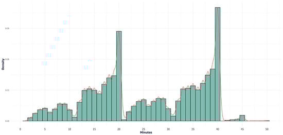
Figure 1.
Distribution of total timeouts requested by game minute.
Segmenting requests by order of timeout, Figure 2 shows that only 27.8% of first-timeout requests occurred in the first quarter, with this percentage increasing to 38.11% in the third quarter. In contrast, second timeout requests are concentrated almost entirely in the second and final quarters, with marginal occurrences in the first quarter (1.98%) and rising to 8.1% in the third quarter, primarily because another timeout is still available. Another notable aspect is that only 30.14% of the second timeouts available in the first half and 25.9% in the second half are used, and of these, only 24.4% result in a third timeout request.
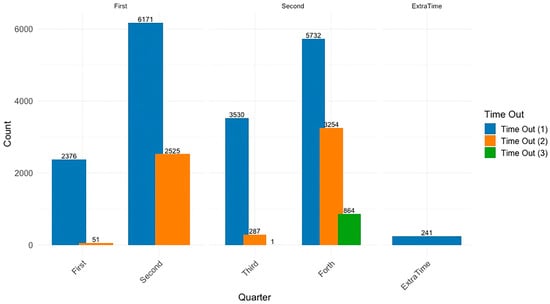
Figure 2.
Distribution of timeouts by quarter and order of request.
Principal Component Analysis (PCA) [67] was used to reduce the dimensionality of the dataset while preserving most of its original variability. Given the complexity of play-by-play basketball data, which includes multiple interdependent variables, high-dimensional datasets can introduce redundancy, noise, and multicollinearity, potentially affecting clustering algorithm performance. By transforming the data into a set of uncorrelated principal components, PCA enhances computational efficiency, improves clustering stability, and minimises the risk of overfitting. Additionally, reducing the number of dimensions while maintaining significant variance facilitates data visualisation and interpretation, making the results more accessible to analysts and coaching staff. The application of PCA ensures that the clustering process is based on the most informative features, improving the reliability of the derived patterns in timeout request analysis. These benefits are particularly relevant in large-scale datasets like ours (over 1.9 million events), where dimensionality reduction not only improves computational efficiency but also enhances clustering robustness and generalisability by focusing the algorithm on the most informative variance structure [45,46,67].
After applying PCA (Figure 3), the first three components captured 69.64% of the total variance, with the first component explaining more than 61%. To determine the appropriate number of components to retain, we followed Kaiser’s criterion, which suggests keeping components with eigenvalues greater than 1 [68]. Based on this rule, we retained three components. These variables were derived from the initial set of 21 quantitative variables coded from play-by-play actions and contextual data. Although PCA improves stability and reduces redundancy in high-dimensional datasets, it necessarily involves a trade-off in the interpretability of the original variables.
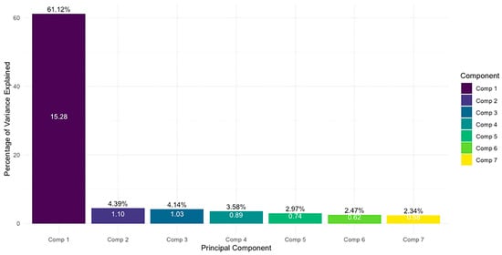
Figure 3.
Distribution of principal components according to the explained variance and eigenvalues.
The three retained principal components reflect key latent structures in the game data:
- PC1 (Scoring and Duration): This component aggregates variables such as minutes played, points scored, field goals made and attempted (2P and 3P), which reflect a team’s scoring activity and overall offensive engagement during the game.
- PC2 (Efficiency and Ball Management): Defined by high contributions from assists, rebounds (defensive and offensive), and turnovers. It captures how effectively the team manages possession and creates opportunities, representing overall game efficiency.
- PC3 (Free Throws and Fouls): Primarily influenced by free throws made/missed and personal fouls, suggesting intensity and rhythm control, often relevant in late-game or high-pressure situations.
These interpretations are supported by the squared cosines visualisation (Figure 4), which shows that key variables such as points, minutes, assists, and free throws are strongly associated with the first two principal components. The representation quality (cos2) confirms that the retained components capture the essential structure of the data, justifying their use in the subsequent clustering analysis.
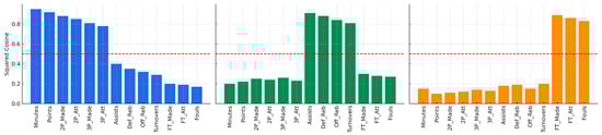
Figure 4.
Squared cosine contributions of variables to PC1, PC2, and PC3. PC1 relates to scoring and game duration; PC2 reflects efficiency and ball control; PC3 captures free throws and fouls.
Additionally, the cosines plot, or correlation coefficients between variables and components (Figure 5), indicates that the quality of representation in the two principal components is high, with most variables—especially minutes played and team scores—well represented in the first two dimensions. Taking all these criteria into account, we retained three principal components for the clustering analysis, as they jointly offer a balance between information preservation and dimensionality reduction while ensuring interpretability and computational efficiency.
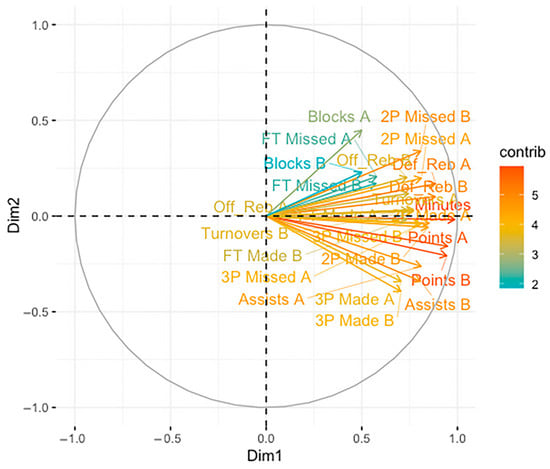
Figure 5.
Plot of variable-component correlation coefficients.
All analyses were conducted using the R programming language (version 4.3.1) within the RStudio (2023.06.1+524) integrated development environment. R was selected for its flexibility, reproducibility, and the availability of advanced statistical and visualisation packages suitable for clustering analysis. Specific libraries used include stats for hierarchical clustering, cluster and factoextra for visualisation and evaluation of clustering quality, and FactoMineR for principal component analysis. This academic use of R ensures transparency and replicability in data analysis, consistent with current best practices in data science research.
4. Results
4.1. Dendrogram Analysis
The visual analysis of the dendrograms [69] (Figure 6) provided insights into the hierarchical structure of the data and the appropriate number of clusters for each method. For most agglomerative methods—particularly Ward.D and Ward.D2—a noticeable increase in linkage distance was observed between the second and third fusion levels, suggesting that the dataset was best represented by two main clusters.
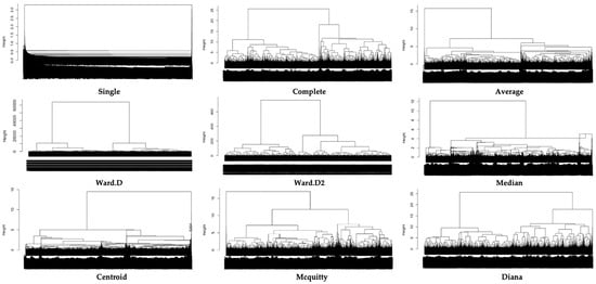
Figure 6.
Plot of variable-component correlation coefficients, Euclidean distance. Although similar patterns were observed across other distance metrics (Manhattan and Minkowski), we only include the Euclidean version here for brevity.
The single-linkage method failed to differentiate the data meaningfully because it grouped nearly all observations into a single chain-like cluster regardless of the distance metric used (Euclidean, Manhattan, or Minkowski). This chaining effect is a known limitation of the proposed method and indicates poor structural separation.
The average-linkage method consistently produced a residual cluster and two larger, well-separated clusters. This structure was stable across the three distance metrics; however, it revealed limited granularity beyond the three clusters.
Complete linkage resulted in three clusters, of which one was consistently marginal in size and composition. This indicates a weaker ability for partition formation than Ward’s method.
Ward.D and Ward.D2 produced two clearly defined clusters with balanced sizes and strong separation, as shown by the clear “elbow” or sharp vertical step in the dendrogram between the second and third fusion stages. These visual cues are suitable for modeling timeout request patterns.
4.2. Cophenetic Coefficients
Figure 7 illustrates the cophenetic coefficients [58] obtained for each method across Euclidean, Manhattan, and Minkowski distances.
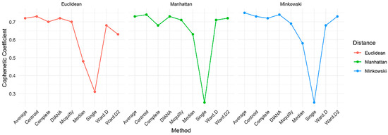
Figure 7.
Cophenetic coefficients by distance and method.
- For the Euclidean distance, centroid (0.73) and average linkage (0.72) achieved the highest coefficients, indicating strong alignment between the dendrogram and the original distance matrix. Complete linkage also performed well (0.70), while Ward.D (0.68) and Ward.D2 (0.63) yielded moderately high values. In contrast, single linkage showed poor structural representation (0.31).
- With the Manhattan distance, the centroid method again yielded the highest coefficient (0.74), followed closely by average linkage (0.73), Ward.D2 (0.72), and Ward.D (0.71). Complete linkage scored 0.68. Single linkage remained the lowest (0.25).
- Under the Minkowski distance, average linkage showed the best performance (0.75), with centroid and Ward.D2 both at 0.73. Complete linkage followed with 0.72, while Ward.D scored 0.68. Single linkage once again had the lowest value (0.25).
Overall, average linkage and centroid methods consistently achieved the highest cophenetic coefficients across all three distances, suggesting that they best preserve the structure of the original data. Ward.D and Ward.D2 also demonstrated reliable performance, particularly with Manhattan and Minkowski distances. Single linkage consistently underperformed, indicating that it is the least effective in preserving original data structure through the dendrogram.
4.3. Silhouette Index
Figure 8 shows the silhouette index values [59] obtained for each configuration.
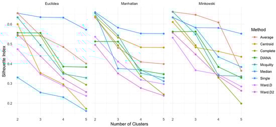
Figure 8.
Silhouette index by distance type, number of clusters, and method.
- For the Euclidean distance, the single-linkage method achieved the highest silhouette score with two clusters (0.6547) and maintained relatively high values as the number of clusters increased, despite a slight decline. The average linkage also demonstrated stable and high performance across the cluster counts. In contrast, Ward.D and Ward.D2 displayed a more significant drop in silhouette values as k increased, reaching 0.2375 and 0.2568, respectively, for the five clusters, indicating weaker cohesion and separation.
- With the Manhattan distance, single linkage recorded the highest silhouette value with two clusters (0.6594) and remained robust (0.5512) at five clusters. Complete linkage also showed strong initial values but notably decreased at higher k. The average-linkage and McQuitty methods remained relatively stable, suggesting good structural performance across cluster numbers.
- For the Minkowski distance, the results were consistent with those of previous metrics: single linkage achieved 0.6547 with two clusters and maintained high values across k. The average linkage again performed well, particularly at k = 2. The median and centroid methods showed greater variability in silhouette scores, reflecting less stable clustering outcomes.
Overall, single- and average-linkage methods consistently obtained the highest silhouette index values across all three distance metrics. These methods are most effective for forming well-defined clusters. The highest silhouette values were generally observed at k = 2, confirming that a two-cluster solution is optimal for most configurations.
4.4. Elbow Method
The Elbow Method [60] was used to identify the optimal number of clusters by analysing the within-cluster sum of squares (WSS) across configurations.
To determine the optimal number of clusters, the Elbow Method was employed as a visual diagnostic tool. This approach involves calculating the total within-cluster sum of squares (WSS) for a range of cluster numbers (k = 1 to 5). The WSS values are plotted against the number of clusters to identify the “elbow” point—where the rate of decrease in WSS begins to flatten—indicating a trade-off between model simplicity and clustering accuracy. In this study, the Elbow Method suggested that k = 2 was the most suitable number of clusters, with a secondary inflection at k = 4. These findings were further supported by additional validation indices such as the Silhouette and Gap Statistic. Figure 9 illustrates the WSS curves for each linkage method and distance metric combination across the k = 2 to 5 range.
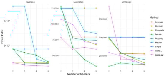
Figure 9.
Elbow method by distance type, number of clusters, and method.
With the Euclidean distance, the Ward.D and Ward.D2 methods showed the most significant decrease in WSS values as the number of clusters increased, dropping to 82,321.2 and 79,840.4, respectively, at k = 5. This steep decline suggests that these methods are more sensitive to increased partitioning. In contrast, single- and average-linkage methods began with high WSS values (430,026.6) and exhibited only moderate reductions across cluster counts, with average linkage decreasing more clearly to 146,240.0 by k = 5.
Under the Manhattan distance, single linkages showed limited reduction in WSS (from 125,356.1 to 125,187.7), indicating that additional clusters had little effect on intra-cluster dispersion. Complete linkage showed a stronger reduction trend, whereas average linkage and McQuitty maintained relatively high and stable WSS values across k, supporting their suitability under this metric.
For the Minkowski distance, both single- and average-linkage methods maintained high WSS values regardless of the cluster number, suggesting more stable cluster cohesion. Conversely, median and centroid methods produced more variable WSS values, reflecting inconsistent clustering structures and lower compactness.
Overall, the Elbow Method results suggest that single- and average-linkage methods maintain more consistent WSS values across cluster counts, particularly for Manhattan and Minkowski distances. However, the Ward.D and Ward.D2 methods demonstrated sharper reductions in WSS under the Euclidean metric, suggesting better partitioning efficiency. In most cases, the elbow was observed at k = 2, which supports the choice of two clusters as optimal for most configurations.
4.5. Gap Statistics
The Gap Statistic [61] was used to evaluate the separation and compactness of clusters compared to a null model of uniformly distributed data. Figure 10 displays the Gap values obtained for each clustering method and distance metric combination.
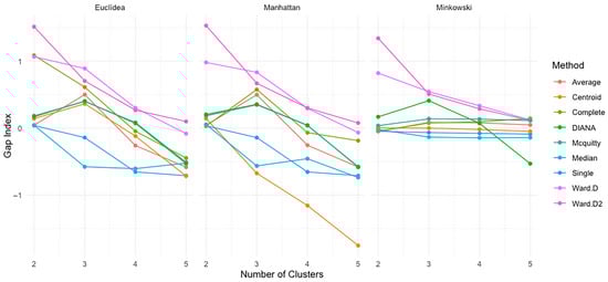
Figure 10.
Gap statistics index by distance type, number of clusters, and method.
For the Euclidean distance, the Ward.D and Ward.D2 methods produced the highest Gap values with two clusters (1.0656 and 1.5132, respectively), suggesting strong cluster separation. In contrast, the single-linkage method showed a much lower Gap value (0.0385) with two clusters, which became negative (−0.1426) when increasing to three clusters, indicating deterioration in the cluster structure. The average linkage maintained positive values across cluster counts, indicating stable performance.
Under the Manhattan distance, the single-linkage method began with a Gap value of 0.0335 at two clusters and slightly increased at three clusters (0.1426), while Ward.D started at a high value (0.9799) and gradually declined to 0.0676 by five clusters. The average-linkage and McQuitty methods also maintained positive Gap values across cluster numbers, indicating consistent clustering performance under this distance metric.
With the Minkowski distance, the single-linkage method yielded a negative Gap value at two clusters (−0.0482), suggesting poor cluster separation. Ward.D achieved a positive value (0.8204) at two clusters and maintained a decreasing but still positive trend as more clusters were added. The median and centroid methods showed greater fluctuation in Gap values, indicating less reliable cluster formation.
Overall, the highest Gap values were obtained using the Ward.D and Ward.D2 methods, particularly under Euclidean and Manhattan distances, thereby reinforcing the quality of two-cluster solutions in those settings. Average-linkage methods consistently performed well across distances, whereas single linkage exhibited instability, especially at Minkowski distances.
4.6. Calinski–Harabasz Index
The Calinski–Harabasz index [62] was used to assess the cohesion and separation of clusters, with higher values indicating better-defined and more compact groupings. Figure 11 shows index values across different clustering methods, distances, and number of clusters (k = 2 to 5).
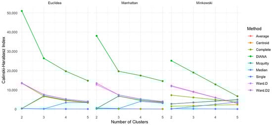
Figure 11.
Calinski–Harabasz index by distance type, number of clusters, and method.
For the Euclidean distance, Ward.D2 achieved the highest index value with two clusters (13,619.78), closely followed by complete linkage (13,440.92) and Ward.D (13,341.64). However, the values dropped significantly as the number of clusters increased, with complete linkage falling to 3554.68 at five clusters, indicating reduced structural clarity.
Under the Manhattan distance, Ward.D2 obtained the highest value with two clusters (13,477.83), followed by Ward.D (12,717.17). Like the Euclidean case, the index decreased steadily for all methods as more clusters were added. Average linkage and McQuitty also demonstrated strong performance in two clusters but experienced notable declines at higher cluster counts.
With the Minkowski distance, Ward.D2 and Ward.D maintained the highest index values with two clusters (12,187.10 and 11,848.41, respectively). By five clusters, the index values dropped substantially; for example, complete linkage reached only 3715.70, and Ward.D fell to 2991.01.
Overall, the highest Calinski–Harabasz values were consistently observed in two clusters, particularly when using the Ward.D and Ward.D2 methods across all distance metrics. These results reinforce the effectiveness of these methods in generating compact and well-separated clusters in the context of timeout event data.
4.7. Davies–Bouldin Index
The Davies–Bouldin index [63] was used to assess the compactness and separation of clusters, where lower values indicate better clustering performance. Figure 12 presents the index values obtained across methods, distances, and cluster counts.
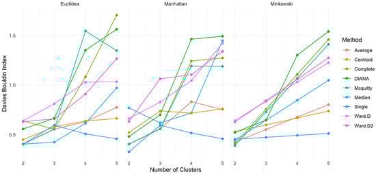
Figure 12.
Davies–Bouldin index by distance type, number of clusters, and method.
With the Euclidean distance, single linkage achieved the lowest index value at two clusters (0.4022), closely followed by average linkage (0.4023), suggesting strong initial cohesion and separation. However, index values increased notably with additional clusters, indicating a weaker clustering structure; for instance, complete linkage rose to 1.7053 at five clusters.
Under the Manhattan distance, single linkage yielded the best result at two clusters (0.3247), but performance declined with more clusters (0.4564 at five). Ward.D started at 0.6603 and deteriorated significantly to 1.4216 with five clusters. Average linkage and McQuitty also showed good performance at two clusters, but their indices increased with the cluster count.
For the Minkowski distance, the single-linkage method produced a higher initial value (0.4516), reflecting weaker compactness relative to other distances. Ward.D and Ward.D2 showed acceptable values at two clusters (0.6399 and 0.6254, respectively), but their performance declined as clusters increased. At the five clusters, complete linkage reached 1.4590 and Ward.D 1.2253, again indicating reduced clustering quality.
Overall, the Davies–Bouldin index supports the use of two clusters as the optimal configuration across all distance metrics. The single- and average-linkage methods showed the best performance under Euclidean and Manhattan distances, while Ward.D and Ward.D2 maintained acceptable values under Minkowski conditions. As with the other indices, the clustering quality decreased as the number of clusters increased.
4.8. Dunn Index
The Dunn index [64] was applied to evaluate the quality of cluster configurations, where higher values indicate greater separation between clusters and lower intra-cluster dispersion. Figure 13 shows the Dunn index values obtained from each method across the three-distance metrics and cluster counts.
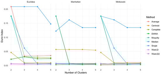
Figure 13.
Dunn index by distance type, number of clusters, and method.
For the Euclidean distance, both single- and average-linkages achieved the highest Dunn index value at both clusters (0.20871), suggesting strong structural quality. The index values decreased substantially as the number of clusters increased. For example, the complete linkage decreased to 0.02704 at the five clusters, reflecting weakened cohesion and separation.
Under the Manhattan distance, single linkage again recorded strong results, starting at 0.12201 with two clusters and increasing slightly to 0.16191 at three clusters. Ward.D started at a much lower value (0.00590) and declined further to 0.00512 by five clusters. The average and McQuitty methods demonstrated solid performance with two clusters but followed a downward trend as k increased.
With the Minkowski distance, the single-linkage method yielded the highest value again with two clusters (0.17512), while Ward.D and Ward.D2 began with low values (0.00491 and 0.00704, respectively) and declined further with more clusters. At the five clusters, complete linkage dropped to 0.00654 and Ward.D to 0.00351.
Overall, the Dunn index results confirmed that the clustering quality was the highest with the two clusters across all distance metrics. The single-linkage method consistently provided the best performance under all conditions, particularly for the Euclidean and Minkowski distances.
4.9. Cluster Size
Cluster size analysis revealed notable differences in balance and distribution among the evaluated methods. Table 2 summarises the number of elements per cluster for each method and distance metric.
Table 2.
Cluster sizes by method.
Across all three distances (Euclidean, Manhattan, and Minkowski), Ward.D2 consistently produced the most balanced clusters, with a relatively even distribution of data points between clusters. This suggests a strong ability to avoid the formation of dominant or marginal clusters.
In contrast, single-linkage and average-linkage methods tend to generate highly imbalanced clusters, often concentrating most data points into one cluster while isolating negligible subsets into another. This imbalance may limit their utility in applications in which equitable representation of cases across clusters is desired.
The DIANA and McQuitty methods offered moderately balanced distributions, performing better than single and average linkage but not as consistently as Ward.D2.
Overall, Ward.D2 demonstrated the greatest effectiveness in maintaining cluster size balance across all distance metrics, making it a suitable choice when balanced grouping is essential for interpretation or subsequent analysis.
4.10. Descriptive Analysis of Clusters
The descriptive analysis focused on the two-cluster solutions obtained with the Ward.D and Ward.D2 methods using the Euclidean distance, which demonstrated strong performance across most internal validation indices and generated well-balanced cluster sizes.
The box score statistics (Table 3) for both clusters were compared, highlighting consistent differences in team performance depending on whether a timeout was requested (TO) or not (NTO).
Table 3.
Mean and median box scores according to the Ward.D method (2 Clusters).
- In Cluster 1, the differences between the TO and NTO teams were relatively small. However, NTO teams recorded slightly better performance in terms of points scored, free throws made, and fewer turnovers, suggesting marginally greater efficiency and control in these game scenarios.
- In Cluster 2, the differences were more pronounced. NTO teams outperformed TO teams in multiple key metrics, including points, assists, free throws, and overall offensive efficiency. This finding suggests that in these game contexts—characterised by longer elapsed time—teams that did not call timeouts were able to maintain more effective and consistent play, especially in ball management and capitalising on scoring opportunities.
Additionally, the average timing of timeouts differed across clusters: in Cluster 1, timeouts were typically requested midway through the second quarter, whereas in Cluster 2, they were more commonly observed midway through the final quarter.
Overall, these results highlight two distinct profiles of game situations: one in which timeouts have limited impact (Cluster 1), and another in which avoiding a timeout appears associated with better in-game performance (Cluster 2).
To complement the previous analysis, Table 4 presents the overall mean and median box score values for each cluster, without distinguishing between whether a timeout was requested or not. This allows for a global assessment of the performance characteristics that define each cluster, independent of team-specific timeout decisions. The results confirm the segmentation already observed: Cluster 1 (n = 11,886 TO) is associated with lower offensive production and fewer accumulated statistics across all indicators, while Cluster 2 (n = 13,145 TO) reflects high-performance game contexts, with markedly higher values in points, shooting attempts, rebounds, assists, and efficiency.
Table 4.
Overall mean and median box scores by Ward.D clustering (2 Clusters).
The similarity between the means and medians in each cluster suggests internally consistent performance profiles. Cluster 1 exhibits moderate activity levels, while Cluster 2 shows a more intensive game phase, likely corresponding to later stages of the game. These findings reinforce the interpretation proposed in Table 3: Cluster 2 corresponds to high-stakes situations where, in many cases, teams that do not call a timeout maintain superior performance.
In the analysis of Clusters 1 and 2 generated by the Ward.D2 method (Table 5) it is observed that the team that does not request a timeout (NTO) performs slightly better than the team that requests a timeout (TO) in several key aspects. In Cluster 1, the differences between both teams are small, but Team NTO shows a slight advantage in points, free throws made (T1C), and defensive rebounds (RD), reflecting greater efficiency and control of the game in more balanced situations.
Table 5.
Mean and median box scores according to the Ward.D2 method (2 Clusters).
On the other hand, in Cluster 2, the differences become more pronounced. Team NTO stands out in points, assists (AS), defensive rebounds (RD), and efficiency, with a more significant advantage over the visiting team. This suggests that, in situations where the game is more prolonged, as seen in the longer playing time of Cluster 2, Team NTO maintains a more consistent and effective performance, especially in terms of ball handling and taking advantage of opportunities in free throws and assists.
As in Cluster 1, Team NTO continues to show greater efficiency in points and overall efficiency (rating). This trend, visible in both the means and medians, reinforces the idea that the local team is more efficient when the game extends. In general, the local team demonstrates better control of the game, especially in the later phases of the match.
The differences in turnovers (PE) and personal fouls (FP) are not significant, indicating that both teams maintain disciplined control of the game.
To complement the previous analysis, Table 6 presents the overall mean and median box score values for the two clusters generated by the Ward.D2 method, without differentiating between whether a timeout was requested or not. This broader view allows for a more general interpretation of the game contexts represented by each cluster. Cluster 1 (n = 14,961 TO) was associated with moderate levels of activity, whereas Cluster 2 (n = 10,070 TO) exhibited significantly higher performance values in almost all metrics. Specifically, Cluster 2 shows notably higher averages and medians in minutes played, points scored, field goal attempts, assists, and overall efficiency, indicating a game phase with greater offensive intensity and output.
Table 6.
Overall mean and median box scores by Ward.D2 clustering (2 Clusters).
The close alignment between the means and medians in each cluster suggests a stable internal consistency in performance. Cluster 1 reflects more balanced or early-game scenarios, while Cluster 2 corresponds to more demanding phases of play, likely occurring in the later stages of matches. These results reinforce the patterns observed in Table 5, where the NTO teams outperformed the TO teams in Cluster 2. The broader analysis in Table 6 validates that Cluster 2 indeed captures high-performance, high-intensity moments in the game, regardless of timeout decisions, adding robustness to the interpretation of strategic game contexts.
In the comparative analysis of the clustering quality indices, we observed that while two clusters offer the best separation and compactness in most cases, opting for four clusters represents a reasonable balance between granularity and clustering quality. Although three clusters are also a solid option, the indices indicate that the difference in quality between three and four clusters is not significant, making four clusters a valid choice if greater segmentation is desired without excessively sacrificing accuracy. In comparison, five clusters show a noticeable decline in quality, suggesting that four clusters are the better option for achieving more detailed partitioning without substantial loss in separation and cohesion among clusters.
In the analysis of Clusters 1 through 4 generated by the Ward.D method (Table 7), the team that does not call a timeout (NTO) generally performs slightly better than the team that calls a timeout (TO) across various metrics, particularly in scoring and efficiency.
Table 7.
Mean and median box scores according to the Ward.D method (4 Clusters).
- In Cluster 1, with timeouts requested in the final minutes of the second quarter, differences between the teams are minimal, yet the NTO team shows a slight advantage in points, free throws made (1P made), and overall efficiency. These differences suggest that even in highly balanced situations, the NTO team exhibits slightly superior scoring effectiveness and game control, as reflected in both the means and medians.
- In Cluster 2, with timeouts requested in the final minutes of the third quarter, the differences become more pronounced. The NTO team outperformed the TO team in points, free throw attempts, assists, and efficiency, showing an advantage in both scoring and ball-handling metrics. The higher efficiency scores and superior performance in free throw attempts suggest that the NTO team maintains a more effective and consistent approach as the game progresses, capitalising on offensive opportunities.
- In Cluster 3, with timeouts requested in the final minutes of the game, the NTO team continues to demonstrate superior performance in points, free throws, and overall efficiency. The scoring advantage and efficiency gap, while not drastic, indicate that the NTO team has an edge in control and effectiveness, particularly in seizing scoring opportunities during extended periods of play.
- In Cluster 4, with timeouts requested in the first quarter, the differences narrowed once again, with the NTO team showing only slight advantages in points and efficiency. This group highlights a more balanced competition between teams, with minimal differences across most metrics, suggesting that in shorter and likely more intense play situations, both teams perform similarly in terms of control and effectiveness.
In all clusters, differences in turnovers (TO) and personal fouls (PF) were generally minor, indicating disciplined play by both teams. However, the consistent advantage of the NTO team in points and efficiency underscores a trend in which the team that refrains from calling a timeout often maintains a slight edge in scoring and overall effectiveness, particularly as game time progresses.
To complement the comparative analysis of timeout and non-timeout team performance, Table 8 presents the overall mean and median box score values across the four clusters generated by the Ward.D method, without distinguishing between team types. This global overview allows the identification of structural patterns that define each game segment. The results confirm the increasing gradient of offensive intensity across clusters: Cluster 1 (n = 9562 TO) and Cluster 4 (n = 2324 TO) represent moderate or limited action scenarios, while Cluster 2 (n = 3320 TO) and especially Cluster 3 (n = 9825 TO) depict more intense and productive phases of the game. Cluster 3 is characterised by the highest values across nearly all indicators—points, assists, rebounds, and efficiency—reflecting high-stakes, end-game contexts.
Table 8.
Overall mean and median box scores by Ward.D clustering (4 Clusters).
The alignment between means and medians indicates strong internal consistency within clusters. Cluster 1 and Cluster 4 represent contrasting profiles: while Cluster 1 exhibits mid-game, moderate-intensity play, Cluster 4 clearly represents brief and low-output phases, likely associated with early game segments or limited player involvement. Cluster 2 serves as a transitional stage, bridging moderate- and high-intensity profiles, while Cluster 3 consolidates peak performance scenarios. These descriptive patterns reinforce the trends observed in Table 7, suggesting that late-game contexts (Cluster 3) are linked to enhanced performance levels and that teams abstaining from calling timeouts often demonstrate superior efficiency in these moments.
In the analysis of Clusters 1 through 4 generated by the Ward.D2 method (Table 9), it can be observed that the team that does not request a timeout (NTO) generally shows a slight performance advantage over the team that requests a timeout (TO) across several metrics, particularly in points and efficiency.
Table 9.
Mean and median box scores according to the Ward.D2 method (4 Clusters).
- In Cluster 1, with timeouts called approximately in the early second quarter or late in the first, the differences between the two teams were minimal. However, Team NTO exhibits a small advantage in points, free throws made (1P Made), and efficiency (+2.5 on average, +3 in median), reflecting slightly higher scoring efficiency and game control even in balanced situations.
- In Cluster 2, with timeouts at the end of the second quarter, the differences become more pronounced. Team NTO outperformed Team TO in points (+1.7 on average, +2 in median), free throws made and attempted, and efficiency (+3.4 on average, +3 in median). This scoring and efficiency advantage suggests that NTO capitalises better on scoring opportunities, likely maintaining more consistent and effective performance as the game progresses.
- In Cluster 3, with timeouts called at the end of the third quarter, NTO maintained a more significant lead, especially in points (+3.1 on average, +3 in median), assists, and efficiency (+6.5 on average, +6 in median). This cluster highlights the sustained control that Team NTO has in scoring and playmaking, demonstrating a clear efficiency advantage as the duration of the game increases.
- In Cluster 4, with timeouts called in the final minutes of the game, Team NTO continues to outperform Team TO in points (+2.1 on average, +3 in median) and efficiency (+4.2 on average, +5 in median). Although the difference in some metrics was smaller compared to Cluster 3, the consistent advantage in scoring and efficiency for the NTO suggests that the NTO maintains an advantage in the later stages of the game, particularly in sustained scoring effectiveness.
Across all clusters, the differences in turnover (TO) and personal fouls (PF) are minimal. However, the consistent advantage of Team NTO in points and efficiency, especially as playing time increases, suggests a trend in which the team that does not request a timeout often holds a slight edge in game effectiveness and scoring capability.
To complement the previous analysis by timeout request, Table 10 summarises the overall mean and median boxscore values across the four clusters generated by the Ward.D2 method, offering a global perspective on game dynamics independent of team behaviour. The clusters present a clear progression in performance intensity: Cluster 1 (n = 5020 TO) reflects low-output, early-game phases; Cluster 2 (n = 6711 TO) corresponds to balanced, mid-game situations; Cluster 3 (n = 3230 TO) captures high-production segments during the third quarter; and Cluster 4 (n = 10,070 TO) consolidates peak-performance moments typical of final-game phases. This segmentation confirms the effectiveness of the clustering structure in distinguishing tactical game contexts.
Table 10.
Overall mean and median box scores by Ward.D2 clustering (4 Clusters).
The close alignment between the mean and median values for each cluster indicates internal cohesion. Cluster 1 represents minimal statistical output, whereas Cluster 4 reaches maximal values. Clusters 2 and 3 illustrate transitional intensities, reflecting the progressive buildup of game momentum and the progressive building of team productivity, respectively. The increasing values across clusters for minutes, scoring metrics, assists, and rebounds suggest that the Ward.D2 method successfully captured both the temporal and tactical escalation within the game. These observations are consistent with the previous analysis in Table 9, reinforcing that Cluster 4 encompasses the most demanding game phases—where teams that avoid timeouts often exhibit better performance.
To complement the conditional analyses by timeout status (Table 3, Table 5, Table 7 and Table 9), we also conducted a global assessment of each cluster’s performance characteristics using the overall mean and median box score values (Table 4, Table 6, Table 8 and Table 10), regardless of whether a timeout was requested. This dual approach allows us to interpret the structural nature of each cluster from both contextual and statistical perspectives. The global tables help define each cluster’s profile—for instance, clusters with higher values in minutes, points, and assists reflect prolonged and high-intensity game phases, whereas clusters with lower values correspond to shorter or less active sequences. The consistency between mean and median values within each cluster also supports the internal coherence of the groups and reinforces the clustering solutions’ interpretability.
5. Discussion
As previously mentioned, timeouts in basketball are key tactical tools that coaches use not only to disrupt the opponent’s momentum but also to restructure offensive and defensive strategies at crucial moments in the game [39]. Identifying patterns in timeout requests is fundamental for understanding coach strategies [38].
The results demonstrate that clustering methodologies such as Ward.D, Ward.D2, and DIANA offer more balanced and consistent clusters in terms of size and separation. This balance is essential to avoid the formation of dominant clusters and ensure that different tactical situations are represented equally, which facilitates the practical interpretation and applicability of the results [39,43,51]. In contrast, while single- and average-linkage methods are consistent in some aspects, they tend to create unbalanced clusters, which can complicate the interpretation of tactical decisions if certain events or types of timeouts are overrepresented in a single cluster [39,54].
Our findings, which are in line with previous studies on the importance of data-driven tactical decisions in elite sports, such as the EuroLeague [33,34], reinforce the notion that clustering methodologies that provide well-defined clusters are crucial for interpreting these decisions. In particular, the Ward.D2 method not only better balances cluster sizes but also captures tactical variations more effectively, which is consistent with previous research suggesting that data-driven tactical decisions can significantly enhance team performance [35].
The selection of an appropriate distance metric is essential to ensure accurate classification of data into clusters that faithfully reflect the different strategies employed during timeouts [4]. In this study, the Euclidean distance was proved to be the most suitable metric for grouping types of timeouts in basketball, effectively capturing spatial variations in tactical decisions. This result is supported by high values for indices such as Silhouette, Dunn, and Calinski–Harabasz, which indicate strong internal cohesion and clear separation between clusters, facilitating tactical interpretation [52,63]. Moreover, low Davies–Bouldin index values further confirmed the suitability of the Euclidean distance, indicating that the clusters were well-separated and compact [45,64].
In comparison, Manhattan distance, while useful in other contexts, did not offer the same level of cohesion and separation in this analysis. This finding is relevant because previous studies have suggested that choosing incorrect distance metrics can lead to misinterpretations of tactical patterns in sports [64]. Euclidean distance performed best overall in terms of internal validation indices, likely due to the relatively balanced distribution and the linear structure of the input variables following PCA transformation. Therefore, its selection reinforces the utility of Euclidean distance in basketball tactical analysis, particularly when the data has been standardised and dimensionally reduced.
The selection of Euclidean, Manhattan, and Minkowski distances was guided by their compatibility with standardised numerical variables and their common use in hierarchical clustering. Other distance metrics such as Mahalanobis or cosine similarity were considered less suitable in this context due to their assumptions or data structure requirements. Nonetheless, future studies may explore their application, particularly in domains where inter-variable covariance or directional similarity is relevant.
Identifying the optimal number of clusters is also critical for capturing the underlying typologies of the timeouts without overfitting the data [46,67]. The analysis of various evaluation indices, such as the Elbow Method, Silhouette, Gap Statistics, Calinski–Harabasz, Davies–Bouldin, and Dunn, consistently demonstrated that the two clusters were optimal. This finding is particularly relevant because it suggests that timeouts in basketball can be effectively segmented into two major categories: defensive interruptions and strategic reorganisations [4,57].
In addition, cluster size analysis reinforces the validity of using two clusters, as methods such as Ward.D2 allow for a more balanced distribution of data. This balance is crucial for interpreting tactical patterns because it prevents a single cluster from dominating the analysis, which could bias the results [51,61]. In the context of timeouts, where tactical decisions must be evaluated fairly, this balance significantly enhances the practical utility of the results [64].
The application of PCA played a key role in enhancing clustering stability by reducing dimensional complexity and mitigating the influence of highly correlated variables. By retaining the most informative components, PCA helped to create a more compact feature space, which in turn contributed to the robustness and interpretability of the clustering structure.
In summary, the analysis of clustering methodologies, distance metrics, and the optimal number of clusters strongly supports the use of two clusters to segment timeout typologies in basketball. This configuration not only provides the best separation and internal cohesion but also facilitates the interpretation of the tactical strategies behind the coaches’ decisions.
Although alternative clustering approaches such as k-means, DBSCAN, or Gaussian Mixture Models (GMM) are widely used, our choice of hierarchical methods responds to the need for a flexible, non-parametric framework that does not require predefining the number of clusters and allows for a full exploration of the nested structure of game situations. This is particularly important in sports data contexts where group boundaries are not clearly known a priori.
The Euclidean distance is the most appropriate metric for this type of analysis because it provides well-separated and compact clusters. Methods such as Ward.D, Ward.D2, and DIANA excel at creating balanced and well-defined clusters, which is crucial for properly interpreting strategic actions within the game context [61,64]. These results not only offer a useful framework for segmenting timeouts in basketball but also provide practical tools for coaches and analysts, enabling them to improve strategic decision-making and optimise the use of timeouts to maximise their impact on game outcomes [38,39,60].
One of the limitations of this study is that although the use of two clusters has proven to be optimal for segmenting timeout typologies in basketball, an analysis with a greater number of clusters could provide more detailed and specific information about tactical variations at different moments in the game. By increasing the number of clusters, it will be possible to identify additional subcategories within timeouts, allowing coaches and analysts to discern with greater precision the strategic nuances behind each timeout request. However, this approach can also result in smaller and less representative clusters, which increases the difficulty of generalising the findings.
In the analysis of timeout typologies using two clusters, a clear division emerged between situations where the team that does not call a timeout (NTO) and the team that does (TO) display consistent differences in points and efficiency. In the first cluster, the differences were minimal; however, Team NTO demonstrated slight dominance in terms of efficiency and free-throw accuracy. This finding suggests that in more balanced game situations, calling a timeout may be associated with slightly lower overall performance in the first half of the game. In contrast, in the second cluster, where the game is approaching its final stages, the differences become more pronounced, showing a trend in which the team that avoids timeouts maintains superior performance in key aspects, such as points and assists.
It is important to note that the observed association between lower timeout usage and better performance should not be interpreted causally. It is equally plausible that teams exhibiting stronger control of the game simply have fewer tactical reasons to request timeouts. Our clustering results describe structural game dynamics rather than the effectiveness or inefficiency of timeout strategies.
With four clusters, the analysis allows for more detailed segmentation of timeout situations, revealing specific scenarios according to the phase of the game. For timeouts called during the first and second quarters, results indicate a slightly superior overall performance for the NTO team, suggesting that the timeout may aim to disrupt the opponent’s momentum. In the third-quarter timeouts, NTO demonstrates an advantage in points and assists, although the difference was not overwhelming compared to Team TO, suggesting that the timeout may be related to strategic decisions by the calling team. In the final cluster, corresponding to timeouts called in the closing minutes, Team NTO continues to lead in points and control, while in the first-quarter cluster, the competition is more balanced, indicating that in these early stages, timeouts may be more related to planning specific plays. This division into four clusters reveals that while the effect of timeouts is less pronounced in the early stages of the game, it intensifies in the later phases, particularly favoring teams that avoid them, which manage to maintain consistent performance and effectiveness until the end of the game. Clusters formed using the Ward.D and Ward.D2 methods show a clear progression from early to late game contexts, with Cluster 1 associated with timeouts in the first quarter and Cluster 4 corresponding to the final minutes of play. The likelihood of timeout requests increases in these later clusters, often in response to higher pressure situations, performance fluctuations, or strategic realignment.
Although this study presents descriptive comparisons of performance metrics between TO and NTO teams across clusters, future research could incorporate statistical hypothesis testing to determine whether these differences are significant. This would strengthen the empirical basis for interpreting timeout-related performance patterns.
This study has limitations that may impact the generalisability of the findings. First, the analysis does not account for the outcomes following each timeout, such as whether the team’s performance improves or declines immediately afterward. Additionally, the study does not differentiate between the sequence of timeouts taken within a game (e.g., first, second, or third timeout), which could affect their strategic purpose and impact. Furthermore, this analysis does not examine potential variations in timeout usage based on coach typologies, which may lead to differences in how timeouts are deployed and their effectiveness.
Furthermore, this analysis does not examine potential variations in timeout usage based on coach typologies, which may lead to differences in how timeouts are deployed and their effectiveness.
We acknowledge the exclusion of external validation indices such as the Adjusted Rand Index (ARI) or V-Measure. These require predefined labels for comparison, which are not available in this unsupervised context. Future studies may incorporate expert-annotated game segments or labeled tactical sequences to enable the use of such indices.
Another of the limitations is that the study does not evaluate changes in team performance immediately before and after timeout events. Incorporating short-term fluctuations—such as scoring runs, possession outcomes, or momentum shifts—would provide more direct evidence regarding the tactical impact of timeouts and should be explored in future analyses. Additionally, while factors timeout decisions, these elements could not be included in the present study due to the lack of quantifiable data. Their integration—potentially through mixed-method approaches or enriched datasets—remains an important direction for future research.
Future research could address these aspects to provide a more comprehensive understanding of the role and impact of timeouts in basketball performance.
Although outlier sensitivity was noted—especially in methods such as single linkage—the present study did not conduct a formal sensitivity analysis. Future work could systematically assess the robustness of clustering configurations under different types of noise or data anomalies, such as extreme performance values or recording errors, to ensure the stability and generalisability of the findings.
These findings suggest that timeout behaviour can be meaningfully segmented using clustering techniques, revealing underlying strategic structures within the game. Coaches and analysts could use this information to anticipate when timeouts are typically most impactful, adjust timeout usage patterns according to team profiles, or evaluate timeout timing in post-game analysis.
6. Conclusions
This study evaluated the effectiveness of hierarchical clustering methodologies for identifying structural patterns in timeout requests in EuroLeague Basketball. The results demonstrate that clustering techniques—particularly Ward.D and Ward.D2 using Euclidean distance—produce well-balanced and interpretable groupings, with two-cluster solutions capturing core distinctions in team performance and timeout dynamics, and four-cluster solutions offering more granular segmentation aligned with different phases of the game.
A consistent finding across all configurations is that teams not requesting timeouts (NTO) often exhibited slightly better performance indicators—such as scoring efficiency, assists, and fewer turnovers—particularly in the later stages of the game. While this should not be interpreted as a causal effect, it highlights a structural pattern in which more stable and effective team performance tends to correlate with a lower reliance on timeouts. These insights are valuable for understanding when and how timeouts are typically used and how their occurrence relates to broader game dynamics.
Methodologically, the study contributes a robust framework that combines Principal Component Analysis for dimensionality reduction with a systematic comparison of clustering algorithms and distance metrics. This approach ensures analytical stability and interpretability, making it adaptable for other applications in sports analytics.
Practically, the findings offer actionable insights for coaching staff and analysts, who can use clustering results to identify critical game segments, evaluate the strategic use of timeouts, and develop scenario-based tactical planning. The results are especially relevant in professional contexts like the EuroLeague, where game management decisions have a significant impact on performance outcomes.
Future research should explore external validation of cluster structures through expert analysis, examine short-term fluctuations before and after timeout events, and incorporate contextual variables such as player fatigue or emotional regulation. By expanding the analytical lens, these efforts can deepen our understanding of timeout strategies and their tactical effectiveness in elite basketball.
Author Contributions
Conceptualisation, J.M.C. and J.M.F.L.; methodology, J.M.C.; software, J.M.C. and E.M.P.; validation, J.M.C., J.M.F.L. and E.M.P.; formal analysis, J.M.C.; investigation, J.M.C., J.M.F.L. and E.M.P.; resources, J.M.C.; data curation, J.M.C.; writing, J.M.C., J.M.F.L. and E.M.P.; visualisation, J.M.C.; supervision, J.M.F.L.; project administration, J.M.F.L. All authors have read and agreed to the published version of the manuscript.
Funding
This research received no external funding.
Data Availability Statement
The data presented in this study are available on request from the corresponding author.
Conflicts of Interest
The authors declare no conflicts of interest.
References
- Mace, F.C.; Lalli, J.S.; Shea, M.C.; Nevin, J.A. Behavioral momentum in college basketball. J. Appl. Behav. Anal. 1992, 25, 657–663. [Google Scholar] [CrossRef]
- Nikolaidis, Y. Building a basketball game strategy through statistical analysis of data. Ann. Oper. Res. 2015, 227, 137–159. [Google Scholar] [CrossRef]
- Lei, G.F. The application of the video analysis system on the basketball training and competitions. Appl. Mech. Mater. 2014, 543, 4702–4705. [Google Scholar] [CrossRef]
- Zhou, Y.; Li, T. Quantitative analysis of professional basketball: A qualitative discussion. J. Sports Anal. 2024, 9, 273–287. [Google Scholar] [CrossRef]
- Demenius, J.; Kreivytė, R. The benefits of advanced data analytics in basketball: Approach of managers and coaches of Lithuanian basketball league teams. Balt. J. Sport Health Sci. 2017, 1, 8–13. [Google Scholar] [CrossRef]
- Çene, E. What is the difference between a winning and a losing team: Insights from EuroLeague basketball. Int. J. Perform. Anal. Sport 2018, 18, 55–68. [Google Scholar] [CrossRef]
- Mandić, R.; Jakovljević, S.; Erčulj, F.; Štrumbelj, E. Trends in NBA and EuroLeague basketball: Analysis and comparison of statistical data from 2000 to 2017. PLoS ONE 2019, 14, e0223524. [Google Scholar] [CrossRef]
- Štrumbelj, E.; Vračar, P.; Robnik-Šikonja, M.; Dežman, B.; Erčulj, F. A decade of euroleague basketball: An analysis of trends and recent rule change effects. J. Hum. Kinet. 2013, 38, 183–189. [Google Scholar] [CrossRef]
- Nunes, H.; Iglesias, X.; Daza, G.; Irurtia, A.; Caparrós, T.; Anguera, M.T. The influence of pick and roll in attacking play in top-level basketball. Cuad. De Psicol. Del Deporte 2015, 16, 129–142. [Google Scholar]
- Mikołajec, K.; Maszczyk, A.; Zając, T. Game indicators determining sports performance in the NBA. J. Hum. Kinet. 2013, 37, 145. [Google Scholar] [CrossRef] [PubMed]
- Cabarkapa, D.; Deane, M.A.; Fry, A.C.; Jones, G.T.; Cabarkapa, D.V.; Philipp, N.M.; Yu, D. Game statistics that discriminate winning and losing at the NBA level of basketball competition. PLoS ONE 2022, 17, e0273427. [Google Scholar] [CrossRef]
- Huyghe, T.; Alcaraz, P.E.; Calleja-González, J.; Bird, S.P. The underpinning factors of NBA game-play performance: A systematic review (2001–2020). Physician Sportsmed. 2022, 50, 94–122. [Google Scholar] [CrossRef]
- Roane, H.S.; Kelley, M.E.; Trosclair, N.M.; Hauer, L.S. Behavioral momentum in sports: A partial replication with women’s basketball. J. Appl. Behav. Anal. 2004, 37, 385–390. [Google Scholar] [CrossRef]
- Sampaio, J.; Lago, C.; Gómez, M.Á. Brief exploration of short and mid-term timeout effects on basketball scoring according to situational variables. Eur. J. Sport Sci. 2013, 13, 25–30. [Google Scholar] [CrossRef]
- Kozar, B.; Lord, R.H.; Whitfield, K.E.; Mechikoff, R.A. Timeouts before free-throws: Do the statistics support the strategy? Percept. Mot. Ski. 1993, 76, 47–50. [Google Scholar] [CrossRef]
- Gómez, M.Á.; Jiménez, S.; Navarro, R.; Lago-Penas, C.; Sampaio, J. Effects of coaches’ timeouts on basketball teams’ offensive and defensive performances according to momentary differences in score and game period. Eur. J. Sport Sci. 2011, 11, 303–308. [Google Scholar] [CrossRef]
- Esteves, P.T.; Mikolajec, K.; Schelling, X.; Sampaio, J. Basketball performance is affected by the schedule congestion: NBA back-to-backs under the microscope. Eur. J. Sport Sci. 2021, 21, 26–35. [Google Scholar] [CrossRef]
- Chen, R.; Zhang, M.; Xu, X. Modeling the influence of basketball players’ offense roles on team performance. Front. Psychol. 2023, 14, 1256796. [Google Scholar] [CrossRef]
- Yamada, K.; Fujii, K. Offensive Lineup Analysis in Basketball with Clustering Players Based on Shooting Style and Offensive Role. arXiv 2024, arXiv:2403.13821. [Google Scholar] [CrossRef]
- Yamada, K.; Fujii, K. Two clusterings to capture basketball players’ shooting tendencies using tracking data: Clustering of shooting styles and the shots themselves. Int. J. Comput. Sci. Sport 2025, 24, 35–55. [Google Scholar] [CrossRef]
- Anıl-Duman, E.; Sennaroğlu, B.; Tuzkaya, G. A cluster analysis of basketball players for each of the five traditionally defined positions. Proc. Inst. Mech. Eng. P J. Sports Eng. Technol. 2021, 238, 55–75. [Google Scholar] [CrossRef]
- Hu, G.; Xue, Y.; Shen, W. Multidimensional heterogeneity learning for count value tensor data with applications to field goal attempt analysis of NBA players. arXiv 2022, arXiv:2205.09918. [Google Scholar] [CrossRef]
- Yin, F.; Hu, G.; Shen, W. Analysis of professional basketball field goal attempts via a Bayesian matrix clustering approach. J. Comput. Graph. Stat. 2023, 32, 49–60. [Google Scholar] [CrossRef]
- Sarlis, V.; Tjortjis, C. Sports analytics: Data mining to uncover NBA player position, age, and injury impact on performance and economics. Information 2024, 15, 242. [Google Scholar] [CrossRef]
- Baouan, A.; Rosenbaum, M.; Pulido, S. An optimal transport based embedding to quantify the distance between playing styles in collective sports. arXiv 2025, arXiv:2501.10299. [Google Scholar]
- Xu, X.; Zhang, M.; Yi, Q. Clustering performances in elite basketball matches according to the anthropometric features of the line-ups based on big data technology. Front. Psychol. 2022, 13, 955292. [Google Scholar] [CrossRef]
- Mateus, N.; Esteves, P.; Goncalves, B.; Torres, I.; Gomez, M.A.; Arede, J.; Leite, N. Clustering performance in the European basketball according to players’ characteristics and contextual variables. Int. J. Sports Sci. Coach. 2020, 15, 405–411. [Google Scholar] [CrossRef]
- Gibbs, C.P.; Elmore, R.; Fosdick, B.K. The causal effect of a timeout at stopping an opposing run in the NBA. Ann. Appl. Stat. 2022, 16, 1359–1379. [Google Scholar] [CrossRef]
- Carta, G.; Favero, C.A.; Maver, A. Do timeouts matter? A study of EuroLeague basketball. SSRN 2025, 1–21. [Google Scholar] [CrossRef]
- Jain, A.K.; Murty, M.N.; Flynn, P.J. Data clustering: A review. ACM Comput. Surv. 1999, 31, 264–323. [Google Scholar] [CrossRef]
- Rokach, L.; Maimon, O. Clustering methods. In Data Mining and Knowledge Discovery Handbook; Springer: Boston, MA, USA, 2005; pp. 321–352. [Google Scholar]
- Wu, X.; Kumar, V.; Quinlan, J.R.; Ghosh, J.; Yang, Q.; Motoda, H.; McLachlan, G.J.; Ng, A.; Liu, B.; Yu, P.S.; et al. Top 10 algorithms in data mining. Knowl. Inf. Syst. 2008, 14, 1–37. [Google Scholar] [CrossRef]
- Sibson, R. SLINK: An optimally efficient algorithm for the single-link cluster method. Comput. J. 1973, 16, 30–34. [Google Scholar] [CrossRef]
- Defays, D. An efficient algorithm for a complete link method. Comput. J. 1977, 20, 364–366. [Google Scholar] [CrossRef]
- Sokal, R.R.; Michener, C.D. A statistical method for evaluating systematic relationships. Univ. Kans. Sci. Bull. 1958, 38, 1409–1438. [Google Scholar]
- Ward, J.H. Hierarchical grouping to optimize an objective function. J. Am. Stat. Assoc. 1963, 58, 236–244. [Google Scholar] [CrossRef]
- Murtagh, F.; Legendre, P. Ward’s hierarchical agglomerative clustering method: Which algorithms implement Ward’s criterion? J. Classif. 2014, 31, 274–295. [Google Scholar] [CrossRef]
- Gower, J.C. A comparison of some methods of cluster analysis. Biometrics 1967, 23, 623–637. [Google Scholar] [CrossRef]
- McQuitty, L.L. Similarity analysis by reciprocal pairs for discrete and continuous data. Educ. Psychol. Meas. 1966, 26, 825–831. [Google Scholar] [CrossRef]
- Kaufman, L.; Rousseeuw, P.J. Finding Groups in Data: An Introduction to Cluster Analysis; John Wiley & Sons: Hoboken, NJ, USA, 1990; pp. 154–196. [Google Scholar]
- Rafsanjani, M.K.; Varzaneh, Z.A.; Chukanlo, N.E. A survey of hierarchical clustering algorithms. J. Math. Comput. Sci. 2012, 5, 229–240. [Google Scholar] [CrossRef]
- Jarman, A.M. Hierarchical Cluster Analysis: Comparison of Single Linkage, Complete Linkage, Average Linkage and Centroid Linkage Method; Georgia Southern University: Statesboro, Georgia, 2020; Volume 29, p. 32. [Google Scholar]
- Nielsen, F.; Nielsen, F. Hierarchical Clustering. In Introduction to HPC with MPI for Data Science; Springer: Cham, Switzerland, 2016; pp. 195–211. [Google Scholar]
- Yim, O.; Ramdeen, K.T. Hierarchical Cluster Analysis: Comparison of Three Linkage Measures and Application to Psychological Data. Quant. Methods Psychol. 2015, 11, 8–21. [Google Scholar] [CrossRef]
- Ran, X.; Xi, Y.; Lu, Y.; Wang, X.; Lu, Z. Comprehensive Survey on Hierarchical Clustering Algorithms and the Recent Developments. Artif. Intell. Rev. 2023, 56, 8219–8264. [Google Scholar] [CrossRef]
- Jaeger, A.; Banks, D. Cluster Analysis: A Modern Statistical Review. Wiley Interdiscip. Rev. Comput. Stat. 2023, 15, e1597. [Google Scholar] [CrossRef]
- Moseley, B.; Wang, J.R. Approximation bounds for hierarchical clustering: Average linkage, bisecting k-means, and local search. J. Mach. Learn. Res. 2023, 24, 1–36. [Google Scholar]
- Emmendorfer, L.R.; de Paula Canuto, A.M. A generalized average linkage criterion for Hierarchical Agglomerative Clustering. Appl. Soft Comput. 2021, 100, 106990. [Google Scholar] [CrossRef]
- Randriamihamison, N.; Vialaneix, N.; Neuvial, P. Applicability and Interpretability of Ward’s Hierarchical Agglomerative Clustering with or without Contiguity Constraints. J. Classif. 2021, 38, 363–389. [Google Scholar] [CrossRef]
- Andronache, I.; Papageorgiou, I.; Alexopoulou, A.; Makris, D.; Bratitsi, M.; Ahammer, H.; Radulovic, M.; Liritzis, I. Can Complexity Measures with Hierarchical Cluster Analysis Identify Overpainted Artwork? Sci. Cult. 2024, 10, 1–24. [Google Scholar]
- Hassani, H.; Kalantari, M.; Beneki, C. Comparative assessment of hierarchical clustering methods for grouping in singular spectrum analysis. AppliedMath 2021, 1, 18–36. [Google Scholar] [CrossRef]
- Giordani, P.; Ferraro, M.B.; Martella, F.; Giordani, P.; Ferraro, M.B.; Martella, F. Hierarchical clustering. In An Introduction to Clustering with R; Springer: Berlin/Heidelberg, Germany, 2020; pp. 9–73. [Google Scholar]
- Dogan, A.; Birant, D. K-Centroid Link: A Novel Hierarchical Clustering Linkage Method. Appl. Intell. 2022, 52, 10501–10524. [Google Scholar] [CrossRef]
- Contreras, P.; Murtagh, F. Hierarchical Clustering. In Handbook of Cluster Analysis; Chapman and Hall/CRC: Boca Raton, FL, USA, 2015; pp. 117–152. [Google Scholar]
- Bu, J.; Liu, W.; Pan, Z.; Ling, K. Comparative Study of Hydrochemical Classification Based on Different Hierarchical Cluster Analysis Methods. Int. J. Environ. Res. Public Health 2020, 17, 9515. [Google Scholar] [CrossRef]
- Patnaik, A.K.; Bhuyan, P.K.; Rao, K.K. Divisive Analysis (DIANA) of Hierarchical Clustering and GPS Data for Level of Service Criteria of Urban Streets. Alex. Eng. J. 2016, 55, 407–418. [Google Scholar] [CrossRef]
- Mwakapesa, D.S.; Mao, Y.; Lan, X.; Nanehkaran, Y.A. Landslide Susceptibility Mapping Using DIvisive ANAlysis (DIANA) and RObust Clustering Using linKs (ROCK) Algorithms, and Comparison of Their Performance. Sustainability 2023, 15, 4218. [Google Scholar] [CrossRef]
- Deza, M.M.; Deza, E. Distances and similarities in data analysis. In Encyclopedia of Distances; Springer: Berlin/Heidelberg, Germany, 2013; pp. 291–305. [Google Scholar]
- Sneath, P.H.; Sokal, R.R. Numerical Taxonomy: The Principles and Practice of Numerical Classification; W.H. Freeman: San Francisco, CA, USA, 1973. [Google Scholar]
- Jain, A.K.; Dubes, R.C. Algorithms for Clustering Data; Prentice Hall: Upper Saddle River, NJ, USA, 1988; pp. 154–196. [Google Scholar]
- Rousseeuw, P.J. Silhouettes: A graphical aid to the interpretation and validation of cluster analysis. J. Comput. Appl. Math. 1987, 20, 53–65. [Google Scholar] [CrossRef]
- Tibshirani, R.; Walther, G.; Hastie, T. Estimating the number of clusters in a dataset via the gap statistic. J. R. Stat. Soc. Ser. B (Stat. Methodol.) 2001, 63, 411–423. [Google Scholar] [CrossRef]
- Caliński, T.; Harabasz, J. A dendrite method for cluster analysis. Commun. Stat. Theory Methods 1974, 3, 1–27. [Google Scholar] [CrossRef]
- Dunn, J.C. Well-separated clusters and optimal fuzzy partitions. J. Cybern. 1974, 4, 95–104. [Google Scholar] [CrossRef]
- Davies, D.L.; Bouldin, D.W. A cluster separation measure. IEEE Trans. Pattern Anal. Mach. Intell. 1979, PAMI-1, 224–227. [Google Scholar] [CrossRef]
- Sampaio, J.; Lago, C.; Drinkwater, E.J. Explanations for the United States of America’s dominance in basketball at the Beijing Olympic Games (2008). J. Sports Sci. 2010, 28, 147–152. [Google Scholar] [CrossRef]
- Jolliffe, I.T. Principal Component Analysis for Special Types of Data; Springer: New York, NY, USA, 2002; pp. 338–372. [Google Scholar]
- Kaiser, H.F. The application of electronic computers to factor analysis. Educ. Psychol. Meas. 1960, 20, 141–151. [Google Scholar] [CrossRef]
- Everitt, B.S.; Landau, S.; Leese, M.; Stahl, D. Cluster Analysis, 5th ed.; Heinemann Books: London, UK, 1974. [Google Scholar]
Disclaimer/Publisher’s Note: The statements, opinions and data contained in all publications are solely those of the individual author(s) and contributor(s) and not of MDPI and/or the editor(s). MDPI and/or the editor(s) disclaim responsibility for any injury to people or property resulting from any ideas, methods, instructions or products referred to in the content. |
© 2025 by the authors. Licensee MDPI, Basel, Switzerland. This article is an open access article distributed under the terms and conditions of the Creative Commons Attribution (CC BY) license (https://creativecommons.org/licenses/by/4.0/).