From Block-Oriented Models to the Koopman Operator: A Comprehensive Review on Data-Driven Chemical Reactor Modeling

Abstract

Some chemical reactors exhibit coupled dynamics with multiple equilibrium points and strong nonlinearities. The accurate modeling of these dynamics is crucial to optimal control and increasing the reactor’s economic performance. While neural networks can effectively handle complex nonlinearities, they sacrifice interpretability. Alternatively, block-oriented Hammerstein–Wiener models and Koopman operator-based linear predictors combine nonlinear representation with linear dynamics, offering a gray-box identification approach. This paper comprehensively reviews recent advancements in both the Hammerstein–Wiener and Koopman operator methods and benchmarks their accuracy against neural network-based approaches to modeling a large-scale industrial Fluid Catalytic Cracking fractionator. Furthermore, Monte Carlo simulations are employed to validate performance under varying signal-to-noise ratios. The results demonstrate that the Koopman bilinear model significantly outperforms the other methods in terms of accuracy and robustness.

1. Introduction

Chemical reactor engineering involves studying reaction kinetics, heat transfer, and mixing effects [1,2] in order to model, control, and optimize industrial chemical processes to ensure their safety, efficiency, and profitability. Advancements in mathematical modeling have made a substantial contribution to this area, benefiting both research and industrial applications. However, this approach suffers from linear approximations, simplified assumptions, computing complexity, uncertainty in parameter estimation, and difficulties in adjusting to dynamic process perturbations. These challenges limit their application in real-time control and optimization [1,3,4], emphasizing the importance of advanced modeling techniques.

From system identification perspectives, the above-mentioned limitation may be circumvented by using data-driven approaches. These methodologies have the capability to accurately describe the system dynamics while handling the complex and strong nonlinearities. Neural networks (NNs) are among the most popular methods for this purpose. Readers are referred to recent reviews on the application of NNs in chemical reactors [5,6] and to [7] for the Fluid Catalytic Cracking (FCC) process. However, statistically mapping inputs to outputs imposes certain constraints on our understanding of the fundamental physical or chemical mechanisms governing reactors. Incorporating prior knowledge into these models can present significant challenges. Consequently, the resulting models may be both complex and elusive in terms of interpretation.

As a response to these limitations, research attention has turned toward block-oriented models, such as Hammerstein–Wiener (HW), and linear predictors for nonlinear systems, specifically the Koopman operator (KO). The motivation behind adopting these methods is their ability to capture and model nonlinear behavior while simultaneously identifying a linear system. This combination of nonlinear and linear behavior gives these methods a flavor of a gray-identification approach. However, to the best of our knowledge, a significant gap remains in the literature: no review to date directly examines how these gray methods have been or could be applied to overcome the above-mentioned limitation while addressing challenges related to the control and optimization of chemical reactors.

The purpose of this paper is twofold. On one hand, it aims to provide a comprehensive survey of block-oriented models for chemical engineering. Block-oriented methods decompose nonlinear dynamics into static nonlinearities in combination with linear dynamics, yielding structures that are both interpretable and amenable to classical linear system analysis. Several reviews have extensively explored these methodologies. Schoukens and Tiels [8] provide a comprehensive survey of block-oriented system identification, including a detailed review of linear approximation methods and the initialization of identification review. Quaranta et al. [9] expanded this scope to review computational intelligence methods, such as genetic algorithms, particle swarm optimization (PSO), and NNs. Moreover, Xavier et al. [10] offer an extensive and generalized overview of block-oriented modeling methods, specifically Hammerstein, Wiener, and Volterra structures, with application in physical systems.

While these reviews provide valuable insights into block-structured system identification, they do not address the practical challenges of applying these methods to chemical reactors, such as handling model invertibility, input–output multiplicity, and the interpretability of internal variables. Additionally, they lack comprehensive coverage of the integration of hybrid and advanced control strategies, including robust MPC, adaptive MPC, Economic MPC (EMPC), and Real-Time Optimization (RTO), with block-oriented models. This paper fills these gaps by reviewing and analyzing recent studies that explicitly address these often-overlooked challenges, emphasizing their critical role in achieving efficient control and optimization in the context of chemical reactors. Furthermore, it highlights advanced hybrid and integrated methodologies and summarizes recent developments in a structured and detailed manner, offering domain-specific value to researchers and practitioners in chemical process modeling and control.

The other purpose is to present a series of recently published applications of KO theory in chemical engineering. This operator offers a complementary approach by replacing nonlinear systems with infinite-dimensional linear systems acting on observables. This framework originates from Koopman’s 1931 work on Hamiltonian dynamics [11,12], and the framework was extended beyond measure-preserving contexts by Mezić and his collaborators [13,14], leading to a significant increase in data-driven finite-dimensional approximations of the KO. Their subsequent work [15] established foundational concepts for control applications.

Several recent reviews have provided broader perspectives on KO. For example, Bevanda et al. [16] reviewed recent advancements from system-theoretical analysis, identification methods, and general extensions to control. Otto and Rowley [17] presented an in-depth survey of numerical methods developed to approximate the KO. Furthermore, Susuki et al. [18] discussed applications in power systems, while vehicular applications were explored by Manzoor et al. [19]. Shi et al. [20,21] examined its application in robotics, and Klus et al. [22] analyzed its applications within complex network systems. Recent work by Li et al. [23] provides an overview of data-driven predictive control methods, focusing extensively on Koopman-based MPC and Data-enabled Predictive Control (DeePC) with attention to chemical process modeling and control.

However, Li et al. [23] primarily focus on Extended Dynamic Mode Decomposition (EDMD) and general machine learning approximators, and they overlook several advanced methods, such as Sparse Identification of Nonlinear Dynamics (SINDy), Physics-Informed Neural Networks (PINNs), Equation Learner (EQL) networks, and deep learning architectures including Variational Autoencoders (VAEs) and Long Short-Term Memory (LSTM) networks. Moreover, they limit their scope to applications of Koopman-based MPC, robust MPC, and Economic MPC, without addressing industrial challenges frequently encountered in chemical processes, namely, hybrid models for multiple operating regimes, adaptive real-time updates, and variable time delays. In contrast, the present work highlights the state-of-the-art data-driven approaches for KO approximation, presents targeted strategies for each practical challenge, and synthesizes the literature into a structured summary, delivering clear recommendations for future research directions.

Finally, this work presents an application benchmark whose purpose is to compare model accuracy, computational efficiency, and robustness under varying signal-to-noise ratios by evaluating block-structured HW, Koopman, and NN models on a large-scale FCC unit.

The remainder of this paper is structured as follows: Section 2 and Section 3 present a comprehensive review on recent work on block-oriented methods and KO-based approaches, respectively, for the modeling and control of chemical reactors. Section 4 focuses on the application of these methods to a large-scale industrial process—the FCC fractionator—and benchmarks their performance against NN approaches under varying signal-to-noise ratios. Finally, Section 5 presents the conclusion, along with remarks and potential avenues for future research.

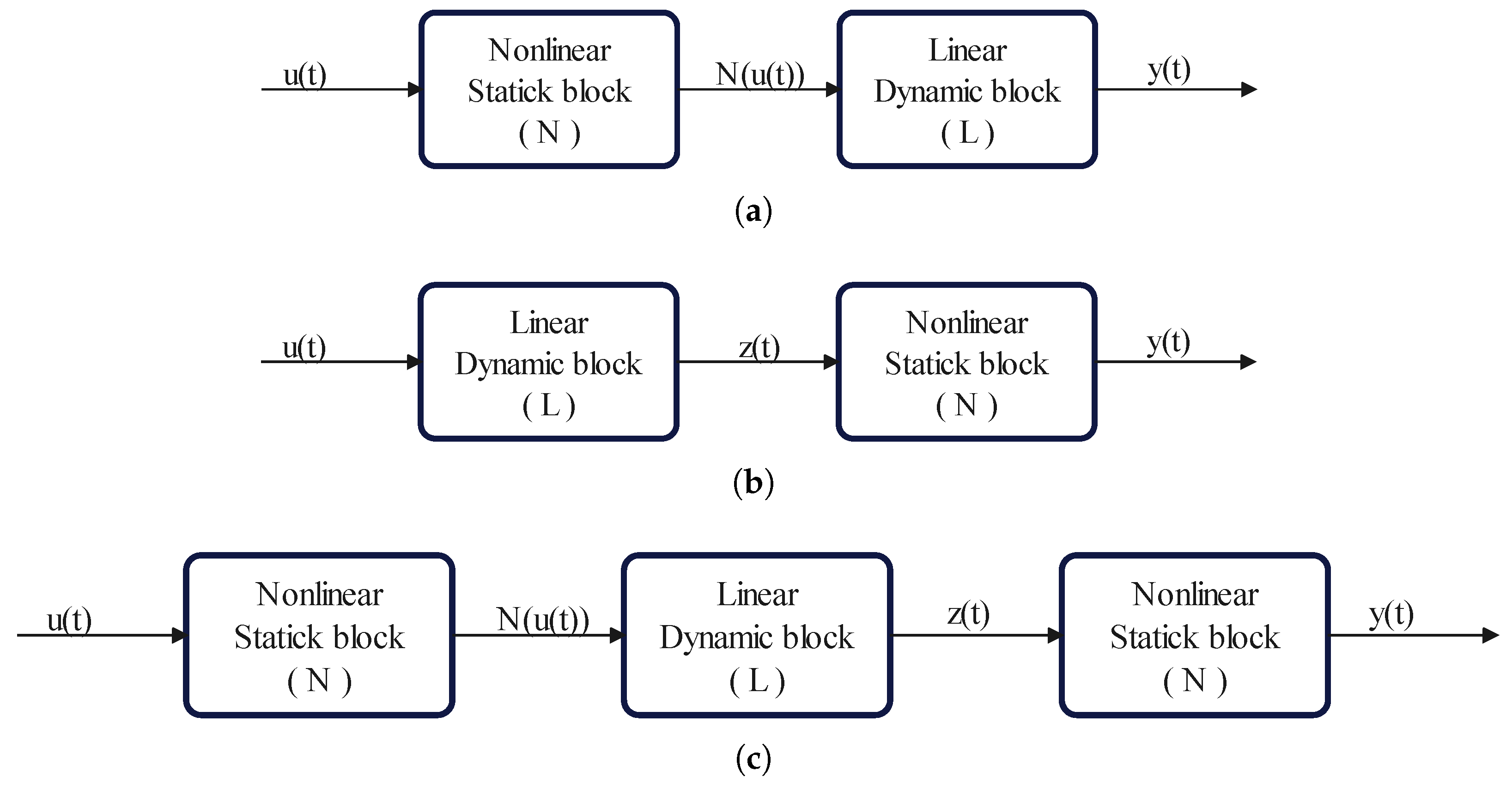
2. Block-Structured Identification

Block-structured models are becoming increasingly popular, as they have demonstrated remarkable results in modeling a broad range of nonlinear systems, for example, solar panels [24], hydraulic systems [25,26] electrical systems [27,28,29], fluid dynamics [30,31], COVID-19 [32], and Stock Price [33]. Typically, the identified system within these models comprises a cascade combination of a static nonlinear input or output transformation blocks and a linear dynamic block. Depending on their order, there are two main classifications of block-structured models: the Hammerstein model and the Wiener model.

The Hammerstein model, first introduced by Hammerstein in 1930 [34], consists of a static nonlinear block $N\left(·\right)$ followed by a linear dynamical system $L\left(·\right)$, as depicted in Figure 1a. The nonlinear block $N\left(·\right)$ captures the various nonlinear phenomena in the inputs of a system, such as actuator nonlinearities. It transforms the input signal $u_k$ into an intermediate variable $v_k$, expressed by $v_k=N\left(u_k\right)$. The linear dynamic block $L\left(·\right)$ then maps $v_k$ to the system’s output response $y_k$. The second structure, called the Wiener model, was originally proposed by Wiener in 1958 [35] and is the dual of the Hammerstein model. It is obtained by reversing the arrangement of the nonlinear and linear blocks, as depicted in Figure 1b. In this structure, the static nonlinear block represents measurement nonlinearities that occur in sensors or affect the system output. In general, the linear dynamical system $L\left(·\right)$ can be approximated using various models of different orders, such as state-space, transfer function, or output-error models. Meanwhile, the nonlinear block $N\left(·\right)$ can be described by various functions, such as dead zones, saturation, or hysteresis functions. More complex models, such as NNs, wavelets, and Piecewise Linear (PWL) functions, can also be used. Combining these two structures results in a Hammerstein–Wiener model, which consists of a nonlinear input transformation, followed by a linear dynamical system, and finally a nonlinear output transformation, as shown in Figure 1c. In the following discussion, the Hammerstein, Wiener, and Hammerstein–Wiener models are denoted by HM, WM, and HWM, respectively.

An early application of the multi-variable HM in FCC was reported in [36,37]. The authors developed a new formulation that preserves both input directionality and multiplicity properties by decoupling the dynamic response of the model in a sparse grid form with respect to all inputs while assuming that the input nonlinearities represent the steady-state behavior. This approach reduced prediction errors by over $50\%$ compared with other HM methods. This method was used in a later work to control the temperature of the FCC reactor using Model Predictive Control (MPC), which resulted in lower errors and reduced computational costs compared with a gain-scheduling controller and a nonlinearity inversion controller [38]. An alternative formulation of the HM, known as IS-Hammerstein, was developed in [39] based on Taylor series expansion of states and inputs. Two applications were used to demonstrate its efficacy: a high-purity distillation column and a Continuous Stirred-Tank Reactor (CSTR). The results showed that the full-order IS-HM accurately captured both systems, while the reduced-order one decreased computation time with acceptable accuracy. The development of an NN-based HM was reported in [40], where the authors used an NN for handling input nonlinearities in order to model the Methyl Tertiary Butyl Ether (MTBE) catalytic distillation process. Compared with the NARX model, this approach achieved higher accuracy in predicting tray temperatures.

Focusing on recursive identification methods, a Recursive Parametric Estimation (RPE) algorithm for HM identification was developed in [41] to adaptively estimate both the dynamic linear and static nonlinear components. The algorithm combines the Recursive Least Squares (RLS) method with the adjustable model approach, and the convergence is proved using the Lyapunov theorem. Tested on an acid–base neutralization process, it demonstrates faster convergence and higher estimation accuracy. Similarly, a recursive kernel-based Hammerstein subspace model for real-time energy efficiency estimation of the ethylene production process was proposed in [42]. The authors in [43] proposed an advanced HM parameter estimation method integrating Stein Variational Inference with Reversible Jump Markov Chain Monte Carlo to improve identification in noisy environments.

Addressing the challenge of nonlinearities within the HM framework, a three-step linearization algorithm was developed in [44] to linearize the PWL functions of the HM, with a lookup table for efficient derivative computation. The objective is to transform the control problem into Quadratic Programming (QP) optimization, eliminating nonlinear function inversion and enabling direct input constraint handling. Simulations on a CSTR and a pH reactor show that the proposed approach achieves similar accuracy to nonlinear MPC (NMPC) while requiring only $5\%$ of the computational time. The study in [45] proposed a self-adjusted decomposition of the HM into local linear models based on the included angle and measurement of nonlinearity in the inputs and used a multi-model MPC strategy for set-point tracking. Compared with previous HM decomposition methods, their approach demonstrated superior control performance and robustness to unmeasured disturbances in a CSTR example.

Expanding upon recursive estimation and HM linearization methods, several researchers integrated the HM into advanced optimization frameworks and adaptive control methods. The paper in [46] proposed a Hybrid Real-Time Optimization (H-RTO) framework that combines HM with an Extended Kalman Filter (EKF) and an adaptive Infinite-Horizon MPC with self-optimizing control. By using transient measurements to continually updating the process parameters, the suggested framework offers enhanced robustness against disturbances, faster convergence, and better economic performance. A least squares support vector machine combined with Laguerre filters was proposed as an HM structure in [47] to simplify nonlinear system identification while improving the performance of MPC for a CSTR. Building on [36,37], the authors in [48] developed a novel HM to handle input interactions and directionality integrated into a single-layer Economic MPC (EMPC) framework that adapts in real time by estimating disturbances and updating model parameters with an EKF. When evaluated on the Williams–Otto reactor, the proposed method outperformed traditional RTO and H-RTO, with improved economic performance and faster computation. The work in [49] proposed a second-order adaptive robust control strategy for proportional pressure-reducing valve (PPRV) control based on an HM. The work in [50] proposed a fractional-order nonlinear Hammerstein control auto-regressive model for heat exchanger process identification using a fractional-order model in the linear block and using fuzzy–genetic algorithms for robust parameter estimation. Similarly, a MIMO fractional-order HM with colored noise was proposed in [51] for improved identification of Proton Exchange Membrane Fuel Cell (PEMFC).

Having reviewed recent HM work, the focus is now shifted to recent developments in WM-based methodologies. The work presented in [52] identified a plug flow reactor process using an NN-based WM for the purpose of temperature control using MPC. In [53], NMPC based on a PWL WM was developed for the control of a polymerization reactor. A continuous-time WM MPC approach for nonlinear systems is presented in [54]; it employs PWL function approximation to handle output nonlinearities. The control law is formulated analytically, combining a constant linear component and a variable nonlinear component, allowing for real-time adaptation without function inversion. Testing on a pH-neutralization process showed that this method outperforms the robust $H_{\infty }$ approach.

Further exploring WM applications, a WM was employed for the identification of a wastewater treatment process in [55] with the objective of optimizing ozone consumption and reducing operational costs. An NN-based WM was developed in [56] for the MPC of an intensified continuous reactor. The authors locally linearized the NN model at each sampling instant, hence transforming the NMPC into linear MPC with varying parameters, which significantly reduces computational complexity. The authors in [57] proposed an adaptive self-tuning controller for the WM, addressing uncertainties and unstable zero dynamics. The method efficiently tracks set-points by combining an inverse nonlinear function block, a modified Clarke criterion, and RLS for parameter estimation. Applied to a CSTR system, the results show the superiority of this method in terms of settling time and robustness over two existing approaches: the inverse NN-based adaptive control presented in [58] and the multiple-model-based adaptive control discussed in [59].

After reviewing the HM and the WM, the attention now is directed towards the latest developments in HWM-based approaches. The authors in [60], developed a low-order HWM to capture the scheduling-related dynamics of an industrial air separation unit for resolving dynamic optimization-based demand response scheduling issues. Their results achieved 13.1% cost savings in real-time markets and 3.6% in day-ahead markets. A double-layered NMPL based on the HWM with a Kalman filter for disturbance rejection was proposed in [61] for offset-free MPC. The authors in [62] proposed an HWM based on NNs and generalized orthonormal basis filters to capture the multiplicity behavior of nonlinear system. Simulations on a continuous fermenter process show that the proposed method outperforms GOBF-NN and NARX-based Deep-NN (DNN) in accurately capturing both dynamic- and steady-state behaviors across various operating conditions. A novel explicit dual adaptive MPC method was developed in [63] based on a discrete-time HWM. The authors in [64] addressed the problem of identifying the HWM in case of infrequent measurements of the output, as encountered in batch processes. First, a nonlinear Dynamic Response Surface Methodology (DRSM) model is identified based on measurements obtained from a set of designed dynamic experiments. The response of this model is then used to generate optimal trajectories, and a local HWM is determined recursively by sampling the DRSM model along these trajectories. Fault-tolerant control based on the HWM was developed in [65,66] for a pressure swing adsorption process to achieve the desired purity while effectively compensating for faults.

Exploring advanced identification techniques and deep learning integrations, an improved version of the HWM was proposed in [67] by combining a spatial–temporal LSTM encoder for measurable disturbances and a Radial Basis Function NN (RBF-NN) observer for unmeasured ones. An MPC method is developed by integrating Nonlinear Prediction and Linearization along the predicted trajectory to control the concentrate grade in an aerial lead–zinc froth flotation process. The work in [68] presented an HWM identification approach for modeling the separation efficiency of a de-oiling hydrocyclone system used in offshore oil and gas production. Additionally, an advanced parameter estimation algorithm for the HWM with unknown time delay was proposed in [69], utilizing the linear variable weight particle swarm optimization (LVW-PSO) algorithm.

The application of block-oriented identification using Hammerstein and Wiener structures has gained significant attention in recent years, leading to notable contributions in the field.

Table 1. Summary of recent work of Hammerstein and Wiener modeling in chemical processes.

Refs.	Process	Linear Model	Nonlinear Model	Approach	Key Highlights
[36,37,38]	FCC	ARX	Polynomials Rigorous model Sparse grid NN	MISO	Multi-variable Hammerstein model for input-directional dynamics and NMPC
[39]	CSTR	Bilinear model	Lookup table	MIMO	Input-state Hammerstein structure for reduced-order modeling
[40]	MTBE distillation	State space	NN	MIMO	Neural Hammerstein model for MTBE distillation control
[41]	Acid–base process	State space	Polynomials	MIMO	Hammerstein-based HRTO with EKF and Infinite-Horizon MPC
[42]	Ethylene production process	State space	Kernel functions	MIMO	Recursive kernel-based Hammerstein model for energy efficiency
[43]	pH neutralization	Transfer function	Polynomials	SISO	Stein Variational Inference for Hammerstein system identification
[44]	CSTR pH neutralization	Transfer function	PWL	MIMO	MPC for PWL Hammerstein systems using online linearization and QP optimization
[45]	CSTR	Transfer function	–	SISO	Self-adjusted decomposition of HM for linear multi-model MPC
[46]	Williams–Otto reactor	Linear ARX	Steady state	MIMO	Hammerstein-based Hybrid RTO based on self optimizing control
[47]	CSTR	Laguerre filters	LSSVM	SISO	LSSVM-L Hammerstein model for improved CSTR control
[48]	Williams–Otto reactor	Transfer function	Gaussian process	MISO	EMPC-based RTO framework using a Hammerstein model
[49]	PPRVs	Transfer function	Polynomials	SISO	Adaptive robust control strategy for PPRVs
[50]	Heat exchanger	Fractional-order difference equation	Polynomials	MIMO	Fractional-order Hammerstein system identification using fuzzy–genetic algorithms
[51]	PEMFC	Fractional-order difference equation	Polynomials	MIMO	Fractional-order MIMO Hammerstein model for PEMFC
[52]	Tubular reactor	State space	NN	SISO	NN-based WM for plug flow reactor identification and NMPC performance evaluation
[53]	Polymerization reactor	State space	PWL	MIMO	NMPC using PWL WM for improved polymerization reactor control
[54]	pH neutralization	State space	PWL	SISO	Continuous-time MPC with PWL approximation for nonlinear systems
[55]	Catalytic ozonation	Transfer function	Polynomials	SISO	Nonlinear WM identification and performance evaluation
[56]	Intensified reactor	State space	NN	SIMO	NMPC with locally linearized NN WM
[57]	CSTR	Polynomials	Polynomials	MISO	Adaptive self-tuning control for uncertain WM
[58]	Air separation unit	State space	PWL	MISO	NN WM for GPC-based nonlinear control
[61]	pH neutralization	State space	PWL	SISO	Double-layered NMPC for offset-free disturbance rejection
[62]	Fermenter system	GOBF-ARX	GOBF-DNN GOBF-SNN NARX-DNN	MISO	GOBF-parameterized HWM using DNN for nonlinear process modeling
[63]	Fermenter system	GOBF	Polynomials	MISO	Adaptive dual NMPC with HWM
[64]	Batch blending process	State space	Polynomials	SISO	Dynamic Response Surface Model for HWM identification
[65,66]	Bio-ethanol dehydration	State space	PWL	SISO	Fault-tolerant control for PSA ethanol purification
[67]	Lead–zinc flotation	Polynomial	NN	MISO	Enhanced HWM with LSTM-based disturbance encoding and observer
[68]	De-oiling hydrocyclone	Transfer function	Polynomials	MISO	Identification of HWM for hydrocyclone separation process
[69]	Circulating fluidized bed boiler	Transfer function	Polynomials	SISO	Simultaneous parameter and time-delay estimation for HWM using LVW-PSO

provides a summary of these works, highlighting key contributions. The identification procedure involves the invertibility of input nonlinearities for the case of Hammerstein or output nonlinearities for Wiener. This enables the translation of set-points, output variables, and their constraints into the intermediate variables within the linear model. However, such transformation is not always feasible and requires the nonlinear transformation to be bijective over the input–output space; thus, input–output multiplicity must be excluded. Hence, the application to multi-variable processes is limited. An attempt to solve this problem for the case of the Hammerstein model was reported in [37], based on Taylor series expansion of input nonlinearities and reformulation of the input signal under the mild assumption that only one input is excited at a time, which might not always be the case. Following the same methodology centered on Taylor series expansion, an output nonlinear function may be linearized as seen in [54,56]. However, neglecting the coupling terms in the expansion would lead to large errors for the case of strongly coupled systems. In addition, these systems may not be easily decomposed into separate SISO systems [45]. Moreover, the choice of input–output nonlinearities and the linear model order is quite challenging and usually depends on a trial-and-error approach. The intermediate variables within the linear model usually do not have a physical meaning and lack interpretability. Fortunately, linear predictors such as the KO theory can help to avoid some of these limitations, which is the subject of the following section.

3. Linear Predictors for Nonlinear Systems

The concept of global linearization of nonlinear systems has consistently held great appeal. In this objective, some linear operators have emerged, namely, the Perron–Frobenius transfer operator [70], the Carleman embedding [71], and the Koopman composition operator [11]. Koopman introduced his operator in 1931 to describe the evolution of measurements in Hamiltonian systems over time [11]. In 1932, Koopman and von Neumann extended this concept to systems with a continuous eigenvalue spectrum [12]. Later, Mezic and his collaborators expanded these ideas to nonconservative systems, laying the groundwork for the application of KO theory in nonlinear system theory [13,14].

The KO is an infinite-dimensional linear operator that describes the evolution of scalar functions, often known as observables, under the dynamics of a nonlinear system. Instead of acting directly on the system’s state space, the KO operates on these observables, capturing the system’s behavior in a function space where the evolution is (approximately) linear. Consider a discrete nonlinear dynamical system:

$$x_{t+1}=f\left(x_t\right),$$

(1)

where $x_t\in \mathcal{X}\subset {\mathbb{R}}^n$ is the state, $\mathcal{X}$ is the state space, and the function $f:\mathcal{X}\to \mathcal{X}$ governs the nonlinear dynamics of the system. The KO $\mathcal{K}$ for (1), defined as an infinite-dimensional operator over a Hilbert space $\mathcal{H}$, advances a set of measurement functions linearly forward in time through the dynamics

$$g\left(x_{t+1}\right)=\mathcal{K}g\left(x_t\right)=g\circ f\left(x_t\right).$$

for every $g:{\mathbb{R}}^n\to \mathbb{C}$ belonging to $\mathcal{H}$. The Koopman Mode Decomposition (KMD) [14] allows one to obtain a decomposition of the KO in terms of its eigenfunctions and eigenvalues, as given by the following equation:

$$\begin{array}{c}\hfill g\left(x_{t+1}\right)={\mathcal{K}}^{t}g\left(x_0\right)=\sum _{i=0}^{\infty }{\lambda }_i^t{\phi }_i\left(x_0\right)v_i^g.\end{array}$$

where ${\lambda }_i\in \mathbb{C}$ is the eigenvalue associated with the eigenfunction ${\phi }_i:{\mathbb{R}}^n\to \mathbb{C}$ and $v_i^g$ is the i-th Koopman mode associated with g.

In the case of a controlled nonlinear dynamical system,

$$x_{t+1}=f(x_t,u_t),$$

(2)

where $f:\mathcal{X}\times \mathcal{U}\to \mathcal{X}$ defines the system dynamics and $u\in \mathcal{U}\subset {\mathbb{R}}^m$ is the control input. The KO for (2) is defined analogously to the operator for the uncontrolled dynamics but evolves in an extended space formed by the product of the state space $\mathcal{X}$ and the space of all control sequences $\mathcal{L}\left(\mathcal{U}\right)=\left\{{\left(u_t\right)}_{t=0}^{\infty }\right|u_t\in \mathcal{U}\}$, denoted by $\mathcal{X}\times \mathcal{L}\left(\mathcal{U}\right)$. The elements of $\mathcal{L}\left(\mathcal{U}\right)$ are denoted by $\mathbf{u}$$:={\left(u_t\right)}_{t=0}^{\infty }$. The dynamics of the extended state, defined as

$${\xi }_t={\left[x_t,{\mathbf{u}}_t\right]}^T,$$

is described by the following equation [15]:

$${\xi }_{t+1}=F\left({\xi }_t\right):=\left[\begin{array}{c}f(x_t,{\mathbf{u}}_0)\\ \mathcal{S}{\mathbf{u}}_{\mathbf{t}}\end{array}\right],$$

(3)

where $\mathcal{S}$ is the left-shift operator, $\mathcal{S}{\mathbf{u}}_t={\mathbf{u}}_{t+1}$, and ${\mathbf{u}}_t$ is the $t^{\mathrm{th}}$ element of the sequence $\mathbf{u}$. The KO $\mathcal{K}$, with respect to (3) is given by

$$\left(\mathcal{K}g\right)\left({\xi }_t\right)=g\left(F\left({\xi }_t\right)\right)=g\left({\xi }_{t+1}\right).$$

for each measurement function $g:\mathcal{X}\times \mathcal{L}\left(\mathcal{U}\right)\to \mathbb{C}$.

It is possible to obtain a finite-dimensional matrix representation of the KO by restricting it to an invariant subspace spanned by a finite set of measurement functions ${\{g_j:\mathcal{X}\times \mathcal{L}\left(\mathcal{U}\right)\to \mathbb{C}\}}_{j=1}^p\subseteq \mathcal{H}$, where each of the functions $g_j$ is well approximated by a finite sum of Koopman eigenfunctions $g_j={\sum }_{j=1}^p{\phi }_j{v}_{ji}^g$ [72]. Consider a vector of measurement functions $\mathbf{g}$ with values in ${\mathbb{C}}^p$:

$$\mathbf{g}(x_t,{\mathbf{u}}_t)={\left[\begin{array}{ccc}{g}_1(x_t,{\mathbf{u}}_t)& \dots & g_p(x_t,{\mathbf{u}}_t)\end{array}\right]}^{\top }.$$

We assume that the measurement function is nonlinear with respect to the state but linear with respect to the input [15,72], i.e.,

$$g_i(x,\mathbf{u})={\psi }_i\left(x\right)+{\mathcal{L}}_i\left(\mathbf{u}\right)$$

and the vector $\mathbf{g}$ is of the form $\mathbf{g}(x_t,{\mathbf{u}}_t)={[\mathit{\psi }\left(x\right),\mathbf{u}\left(0\right)]}^{\top }$, where $\mathit{\psi }={[{\psi }_1,\dots {\psi }_p]}^{\top }$. By focusing the dynamics on the state measurements ${\psi }_i\left(x\right)$, a linear predictor (KL) can be derived [15,72]:

$$z_{t+1}=A{z}_t+B{u}_t,$$

(4)

where $z\in {\mathbb{R}}^p$ is the lifted state, given by

$$z:={\mathit{\psi }}^{\top }\left(x\right)={\left[\begin{array}{ccc}{\psi }_1\left(x\right)& \dots & {\psi }_p\left(x\right)\end{array}\right]}^{\top }.$$

The state $x_t$ is often included in the measurement, e.g., $z={[x^T,\mathit{\psi }]}^T$, so that $x_t$ can be easliy retrieved as

$$x_t=C{z}_t,C=[I_{n\times n},0].$$

Likewise, assuming that one can write $g_i$ as [15]

$$g_i(x,\mathbf{u})={\psi }_i\left(x\right)+{\psi }_i\left(x\right){\mathcal{L}}_i\left(\mathbf{u}\right),$$

a bilinear predictor (KB) can be obtained as [15,72,73]

$$z_{t+1}=A{z}_t+\left(B{z}_t\right)u_t.$$

(5)

Over recent years, there has been significant interest in the data-driven identification of Koopman models. The authors in [74] proposed a data-driven approach for analyzing the Region of Attraction (ROA) of an anaerobic digestion process using the KO. The authors in [75] proposed a data-driven state estimation method integrating linear moving horizon estimation (MHE) based on the KO, which transforms nonlinear state estimation into a convex optimization problem. In [76], EDMD was used to identify and control a CSTR Lyapunov-based MPC, outperforming both the local linearization and subspace identification methods. The authors in [77] proposed a fast Koopman MPC algorithm for Organic Rankine Cycle (ORC)-based Waste Heat Recovery (HWR) process using Hessian matrix invariance in QP, using singular value decomposition to reduce the computational burden.

However, in many practical chemical processes, steady-state offsets and unmodeled disturbances can degrade the performance of nominal Koopman MPC. To address this issue, the work in [78] proposed offset-free MPC based on the KO to control the Kappa number and cell wall thickness of fibers in a batch pulp digester process. The same authors augmented the disturbance dynamics into the Koopman model [79] and developed an offset-free MPC integrating a target optimization problem, a disturbance estimator, and an optimal control problem. This structure allows the Lyapunov function and stabilizing law to be updated in accordance with the desired equilibrium point. Simulation results on a CSTR demonstrated the efficacy of the proposed framework in mitigating the error between the model and the process, surpassing the performance of the nominal Koopman-based MPC. A fuzzy compensation–Koopman MPC method for pressure regulation in Proton Exchange Membrane (PEM) electrolyzers was proposed in [80]. The authors integrated a fuzzy logic compensator to address model mismatch, significantly improving tracking performance. Their approach was compared with nominal Koopman MPC, NN-MPC, and successive linearization MPC, demonstrating superior accuracy and stability.

While offset-free and fuzzy-compensated strategies mitigate steady-state offset, processes with multiple distinct operating regimes or very large state dimensions require more specialized frameworks. In [81], a hybrid MPC framework with multiple Koopman Reduced-Order Models (ROMs) was developed and integrated in closed-loop control using a model-switching methodology. A reduced-order Koopman linear model was developed in [82] by integrating Kalman-based Generalized Sparse Identification (Kalman-GSINDy) to select lifting functions and Proper Orthogonal Decomposition (POD) for dimensionality reduction. Robust MPC built on this model improves computational efficiency by $44\%$ while maintaining high accuracy compared with full-order Koopman MPC. Similarly, a reduced-order Koopman bilinear model based on the Krylov-subspace model reduction method was developed in [83] for NMPC of demand response in chiller plants. The NMPC formulation is further transformed into a convex optimization problem using McCormick relaxation and Chebyshev approximation for demand charge minimization.

Considering the time-varying dynamics and the strongly coupled variables of chemical processes, the offline trained Koopman models may encounter performance limitations when implemented online. To address this issue, the work in [84] proposed an adaptive Koopman modeling framework that integrates SINDy [85] with sparse regression and feature selection. The proposed method outperforms conventional SINDy by achieving higher accuracy with fewer data samples. A data-driven quasi-linear parameter varying (QLPV)-based MPC framework for identification and control of an ORC-based HWR process was proposed in [86], with an online model update mechanism. The approach achieves a root mean squared error approximately 20 times smaller than that of traditional models while also reducing cost and reduces tracking errors by over $97\%$ even in the presence of disturbances.

In addition to time-varying dynamics, some processes often involve unknown or variable time delays, which can critically affect control performance. In this context, a novel Hankel Alternative View of Koopman (HAVOK)-based MPC for time-delay systems with unknown delays was developed in [87]. The authors developed a low-order dynamic model of a District Heating System (DHS) using the HAVOK method and demonstrated accurate prediction and tracking performance. Extending to time-varying operation regimes, a Koopman-based EMPC method for time-varying operation regimes was proposed in [88]. A novel KO-based multi-model MPC method was proposed in [89]; it uses independent sub-models for each sampling step in order to avoid error accumulation in recurrent use. Three variants were presented: (1) with constant matrices, (2) with time-varying linear functions, and (3) with time-varying monomial-based matrices. The results revealed that the time-varying linear models (Model 2) outperform traditional Koopman-based and nonlinear MPC methods.

Moreover, recent work focused on improving the identification of KO and the selection of observable functions. An enhanced EDMD algorithm was developed in [90], featuring a novel eigenfunction construction method to improve the accuracy and interpretability of the Koopman model. The results demonstrated optimized glycerol feed and enhanced production of 1,3-propanediol. The work in [91] proposed an optimization method for selecting Koopman observables in data-driven modeling, using genetic algorithm and differential evolution.

Despite the recent progress, one of the primary challenges in approximating KO lies in the selection of finite basis functions when using methods like EDMD or SINDy, since the accuracy of the model is particularly dependent on the choice of the embedding functions. As there is no universal criterion available for constructing the dictionary of embedding functions, the selection depends on both the specific system under study and the information one aims to capture [72]. This is guided by a combination of domain knowledge, a deep understanding of the dynamical system, and a trial-and-error approach. Indeed, this tedious endeavor can be alleviated through the lens of NNs, as they possess the capability to automatically learn and extract relevant features from data. This motivates the use of NNs to learn the embedding functions of the KO [92,93,94]. In this context, the authors in [95] implemented a Deep NN in order to identify a Koopman-invariant subspace and approximate a linear representation of a Fluidized Bed Spray Granulation (FBSG) process. A linear quadratic integral controller was employed to stabilize the particle size distribution across various operating points. Similarly, the work in [96] developed a reduced-order Koopman model using an Encoder–Decoder DNN. The encoder maps the state space to a lower-dimensional embedded space, while the decoder approximates its inverse. From another perspective, the decoder acts as the output nonlinear transformation in a WM, resulting in the Wiener-Type Koopman model. In terms of accuracy and achievable reduction order, the low-order Wiener-Type Koopman model exhibited superior performance compared with both the linear and bilinear Koopman models. However, one limitation of this method is the need to transform state constraints by using the approximate inverse of the encoder. Additionally, the reduced-order model might not incorporate the state of the system, which limits the physical interpretability of the model. A novel approach for learning the Koopman dynamics is proposed in [97], where the authors extend Koopman theory by incorporating control inputs, allowing for optimal control design via state-dependent Riccati equations. The authors in [98] conducted a comparison between the performance of a Koopman model and a NARX-NN under different experimental conditions using closed-loop data from a Crude Distillation Unit (CDU). The authors in [99] developed a novel Deep Koopman Variational Autoencoder for process monitoring and anomaly detection in industrial biosystems.

Expanding the scope of KO applications, a Koopman-linearized LSTM-based MPC approach was proposed in [100] for real-time control of an electrochemical CO₂ reduction reactor. The reactor dynamics were modeled using an LSTM network, and the KO was applied for online linearization, transforming NMPC into a QP problem. The work in [101] developed a Koopman-based deep integral input-to-state stability bilinear parity approach for data-driven fault diagnosis. A DNN is used to learn the Koopman observables enforcing input-to-state stability constraints simultaneously with the KO in a three-step training process. A novel data-driven modeling approach that integrates an autoencoder-like NN with the KO to develop a semi-linear state-space model for MPC was developed in [102]. The proposed method outperforms traditional methods, offering better set-point tracking, reduced computational time, and improved robustness over the NN-based KO and classical Koopman-based models. A DNN-based KO modeling and analysis method for the anaerobic–anoxic–oxic process in wastewater treatment plants was proposed in [103]. The work in [104] proposed a Deep Input–Output KO for EMPC in wastewater treatment plants, achieving superior performance compared with a benchmark EMPC method. A Deep Recurrent KO framework was proposed in [105] for modeling and controlling uncertain nonlinear systems with time delay based on probabilistic LSTM observables. The proposed method outperforms existing Koopman-based methods in both modeling accuracy and control performance. An input-augmented Koopman modeling and control framework was proposed in [106]. This approach improves the modeling accuracy by explicitly accounting for the nonlinear dependence of lifted state variables on system inputs using two DNNs. However, this resulted in a non-convex MPC problem, which the authors address through an iterative convex optimization algorithm.

These studies demonstrate the feasibility and potential of DNN-based Koopman approaches in learning the Koopman observables, linearizing dynamics, or reducing high-order systems. However, certain processes have well-known physical or mechanistic relationships that can further guide the learning of Koopman models, thereby improving efficiency and interpretability. The work in [107] proposed a multi-stage Koopman approach combined with PINNs in order to accurately model a microbial fermentation process. The authors first applied a fuzzy c-means clustering to divide the process into growth stages and then employed the PINN-based KO to represent the system dynamics for each stage, resulting in an improvement in prediction accuracy. Similarly, a PINN-based Koopman modeling approach was proposed in [108]. The method employs two NNs—a state lifting network for nonlinear lifting functions and a noise characterization network for system noise modeling—leading to a stochastic Koopman model. Furthermore, to improve computational efficiency and eliminate manual tuning, a self-tuning MHE method adaptively updates weighting matrices based on learned noise patterns. In a different approach to learning the observables of the KO, the authors in [109], proposed an interpretable method that integrates Equation Learner (EQL) networks into autoencoders, providing explicit symbolic equations instead of traditional deep learning-based representations. The work in [110] proposed an end-to-end Reinforcement Learning (RL) approach to training Koopman-based (E)MPC for control tasks, thereby achieving superior performance compared with traditional methods. A summary of recent research on the KO in chemical reactors is presented in

Table 2. Summary of recent research on Koopman operator in chemical reactors.

Ref.	Process	Approach	Key Highlights
[74]	Anaerobic digestion	EDMD	Koopman-based ROA classification for anaerobic digestion
[75]	Four-CSTR quadruple water tank	EDMD	Koopman-based constrained MHE for nonlinear state estimation
[76]	CSTR	EDMD	Koopman Lyapunov MPC for stable nonlinear control
[77]	ORC-based HWR	EDMD	Koopman-based fast MPC for ORC
[78]	Batch pulp digester	EDMD	Offset-free Koopman MPC via EDMD for batch pulping
[79]	CSTR	EDMD	Offset-free Koopman MPC with disturbance compensation
[80]	PEM Electrolyzers	EDMD	Fuzzy-compensated Koopman MPC for PEM electrolyzers
[81]	Pulp digester	EDMD	Hybrid KMPC using multiple Koopman-based EDMD models
[82]	Reactor separator	Kalman-GSINDy	Reduced-order Koopman MPC with Kalman-GSINDy and POD
[83]	Chiller plant	SINDyC	Koopman bilinear form NMPC with Krylov model reduction
[84]	CSTR	SINDy	Adaptive Sparse Identification for real-time nonlinear modeling
[86]	ORC-based HWR	EDMD	Koopman-based QLPV model and iterative MPC for ORC-based HWR
[87]	DHS	EDMD	HAVOK-MPC for unknown delay systems
[88]	CSTR	EDMD	Koopman-based EMPC for time varying nonlinear control
[89]	Polymerization reactor	EDMD	Koopman-based multi-model MPC with time varying dynamics
[90]	Fed-batch fermentation	Enhanced EDMD	Enhanced EDMD based on data-driven construction of eigenfunctions
[91]	CSTR	EDMD	Optimization-based Koopman observable selection
[95]	FBSG	DNN	Koopman-based linearization using DNN
[96]	CSTR High-purity methanol–propanol distillation column	DNN	Wiener-type Koopman models for MIMO system identification
[97]	CSTR	DNN	Deep learning-based Koopman transformation for nonlinear system identification
[98]	CDU	DNN	Koopman model identification and assessment for CDU
[99]	Biological process	DNN-based DMD	Deep Koopman-VAE for process monitoring
[100]	Electrochemical CO2 reduction reactor	EDMD	Koopman-linearized LSTM-based MPC for electrochemical control
[101]	Three-tank system	DNN	Koopman-based deep bilinear parity fault detection and isolation
[102]	CSTR	DNN-based DMDc	Autoencoder-enhanced Koopman semi-linear state-space model for efficient MPC
[103]	Anaerobic–anoxic–oxic process	DNN-based EDMD	Koopman-based deep learning for modeling and analysis
[104]	Wastewater treatment	DNN	Deep Input–Output Koopman-based EMPC for wastewater treatment optimization
[105]	CSTR	DNN	Koopman-based learning and control for time-delay systems
[106]	Reactor separator biological wastewater treatment	DNN	Deep learning-enhanced Koopman model with input augmentation
[107]	Microbial fermentation	PINNs	Multi-stage Koopman modeling using PINNs
[108]	Reactor separator	PINNs	Physics-informed Koopman modeling with self-tuning MHE
[109]	CSTR	EQL	Interpretable KO via EQL network
[110]	CSTR	RL	End-to-end RL for Koopman-based MPC optimization

.

Ongoing research continues to refine the application of KO methods for broader industrial applications. The progress summarized here confirms Koopman-based frameworks as a powerful, scalable alternative to classical nonlinear methods—one that can drastically reduce computational burdens without sacrificing performance, stability, or real-time feasibility. Future research directions may consider addressing distributed algorithms for Koopman-based subsystem modeling and control for large-scale industrial plants or multi-unit processes, in which multiple Koopman models coordinate via distributed optimization or cooperative MPC. Moreover, the application of robust Koopman-based MPC and real-time adaptive Koopman-based MPC is still at an early stage. Further research is needed to ensure such adaptation is conducted safely (e.g., using robust identification techniques) and determine appropriate triggers for model updates (to avoid constant retraining). Additionally, papers exploring EMPC and demand response highlight the potential for broader integrated objectives (energy optimization, carbon footprint minimization, etc.), pushing Koopman-based methods beyond purely regulatory control.

4. Application to Large-Scale Processes: Fluid Catalytic Cracking Fractionator

This section explores the use of block-oriented techniques alongside the KO framework to model a large-scale industrial FCC fractionator process and compares their performance against a neural network approach. The robustness of these methodologies is then assessed by evaluating their performance under different signal-to-noise ratio (SNR) levels. The following subsection presents an overview of the FCC process and details the data source.

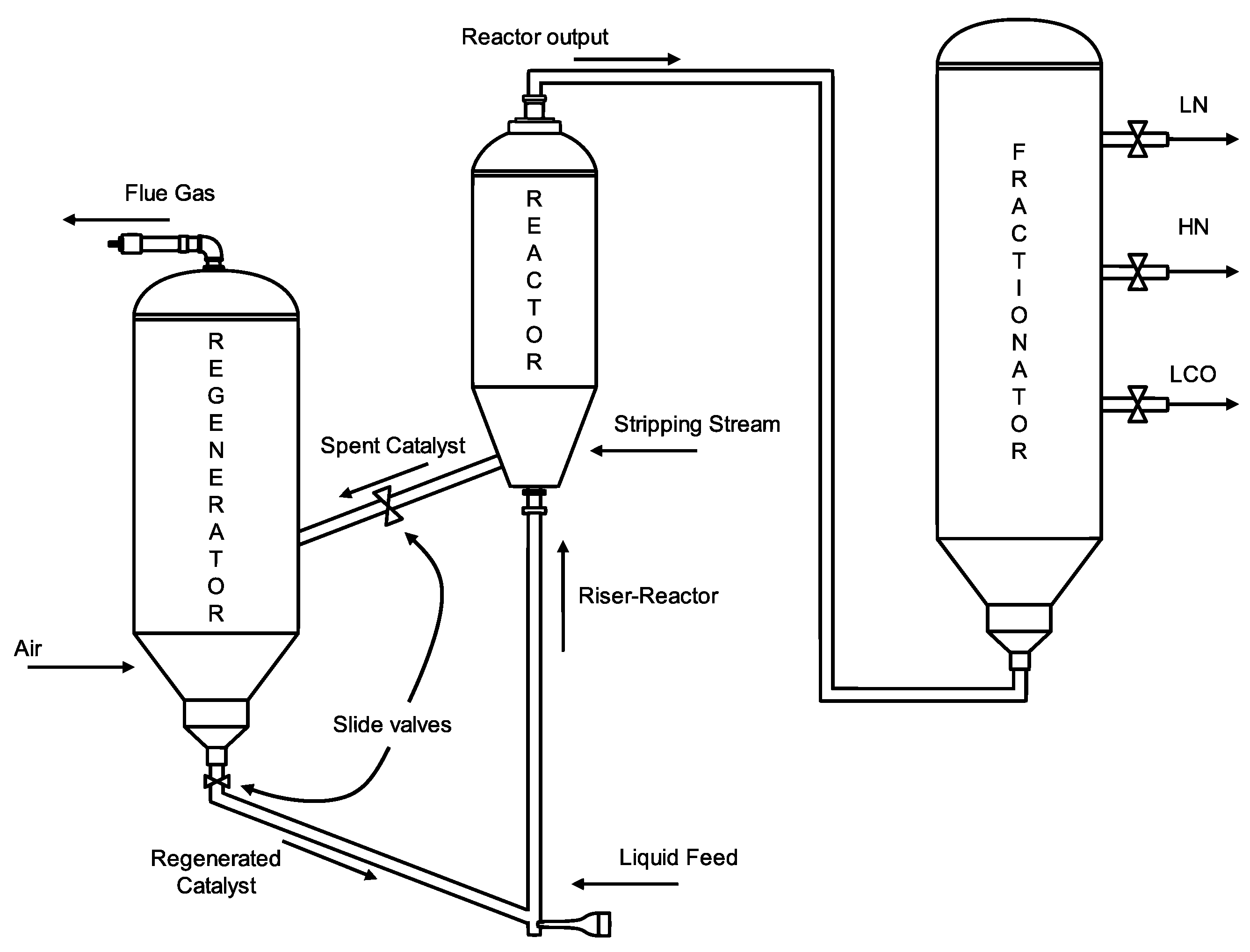
4.1. Fluid Catalytic Cracking Process Overview

FCC is a key process in petroleum refining consisting of three main components: the riser/reactor, the regenerator, and the disengaging vessel [111]. Feedstock is preheated and combined with hot regenerated catalysts in the reactor/riser, leading to rapid conversion of the feedstock into lighter hydrocarbons. This produces undesired coke, deactivating the catalyst. The regenerator uses controlled combustion to burn carbon deposits and regenerate the catalyst, providing the necessary heat for the FCC process. The output from the reactor is directed to the fractionator, which separates it into different products. For a more comprehensive understanding of the FCC process, readers should refer to [111,112]. A schematic representation of the FCC is provided in Figure 2.

To obtain data-driven models for the FCC unit, process data were generated by simulating the open-source FCC fractionator model by Santander et al. (2022) [113] for 83 continuous days at one-minute sampling intervals, yielding $119,520$ samples. Hold-out cross-validation was used to split the data into $50\%$ for training, $30\%$ for validation, and $20\%$ for testing, with the initial state known for each set. During the simulation, each of the manipulated variables (see Table 1 in [113]) was randomly perturbed in magnitude and at different timings. In this work, the valve positions serve as the input u, while the FCC states x include the flow, temperature, pressure, and level profiles in the reactor, regenerator, and fractionator, as listed in

Table 3. List of FCC states and inputs.

Input		State
$V_1$	Flow of fuel	$T_{pre}$	Temperature of fresh feed entering the reactor
$V_2$	Flow of regen. cat.	$T_{rea}$	Temperature of reactor/riser
$V_3$	Flow of spent. cat.	$P_{rea}$	Reactor pressure
$V_6$	Flow of air	$L_{rea}$	Catalyst inventory in reactor
$V_7$	Flow of flue gas	$T_{reg}$	Temperature of regenerator
$V_4$	Flow of LPG	$P_{reg}$	Regenerator pressure
$V_9$	Flow of LN	$L_{reg}$	Catalyst inventory in regenerator
$V_8$	Flow of reflux	$P_{fra}$	Fractionator overhead pressure
$V_{10}$	Flow of HN	$L_{fra}$	Fractionator accumulator level
$V_{11}$	Flow of LCO	$T_{fra}$	Fractionator overhead temperature
		$T_{hnt}$	HN $98\%$ cut point
		$T_{lco}$	LCO $98\%$ cut point

. Data preprocessing was kept to a minimum to preserve the original dynamics of the simulated process; there were no missing values or outliers, and no additional filtering, smoothing, or data augmentation techniques were applied. All inputs and states were standardized to zero mean and unit variance prior to model fitting. The mean squared error (MSE) was used to evaluate model performance, as it provides a straightforward, interpretable measure of the average squared deviation between predicted and true state values—making it ideal for quantifying and comparing regression accuracy. Bayesian optimization was employed to tune each model’s parameters to minimize the average MSE across all states. Details for each of the data-driven models employed in this study are provided in the following subsections.

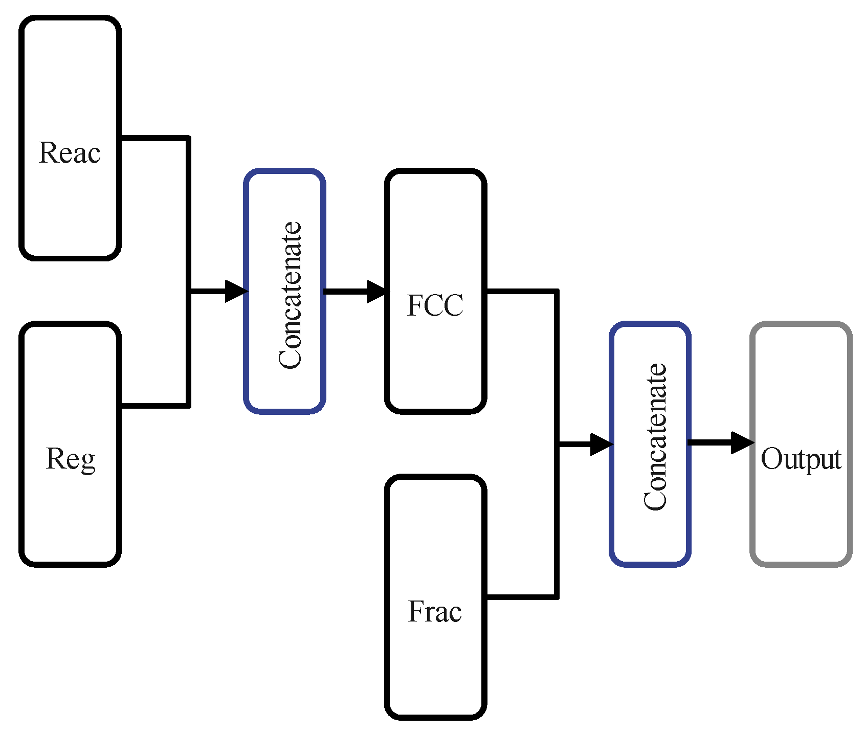
4.2. Multi-Headed Long Short-Term Memory Neural Network

A Multi-Headed (MH-LSTM) architecture was adopted from our recent work on FCC process modeling [114]. In this approach, manipulated-variable and state signals are first grouped according to the FCC unit’s sections—reactor, regenerator, and fractionator—and each group is fed into a dedicated LSTM “head” to extract section-specific temporal features. The outputs of these three LSTM heads are then concatenated and passed through a fully connected layer to yield the final state prediction. This structure mirrors the physical layout of the FCC unit, enables targeted feature learning, and has been shown to improve predictive accuracy over other architectures [114]. The network topology is depicted in Figure 3. The model was trained using MSE as the loss function, minimizing the error between the predicted and actual states.

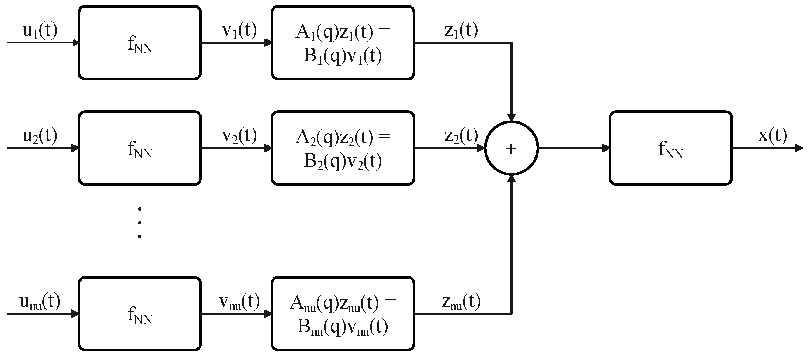
4.3. Hammerstein–Wiener Model

In this work, a Multi-Input Single-Output HWM is developed, as illustrated in Figure 4 and defined by the following equations:

$$\begin{array}{cc}\hfill & v_i\left(t\right)=f_{\mathrm{INN}}\left(u_i\right),\hfill \end{array}$$

(6a)

$$\begin{array}{cc}\hfill & A_i\left(q\right)z_i\left(t\right)=B_i\left(q\right)v_i\left(t\right),\hfill \end{array}$$

(6b)

$$\begin{array}{cc}\hfill & x\left(t\right)=f_{\mathrm{ONN}}\left(\sum z_i\left(t\right)\right).\hfill \end{array}$$

(6c)

where $f_{\mathrm{INN}}\left(·\right)$ and $f_{\mathrm{ONN}}\left(·\right)$ in (6a) and (6c) are static feed-forward NNs for input and output nonlinearities, respectively, and $v_i$ and $z_i$ are the corresponding intermediate variables. The linear dynamics in (6b) are expressed in the backward-shift operator $q^{-1}$, with

$$\begin{array}{cc}\hfill & A_i\left(q\right)=1+a_i^1{q}^{-1}+a_i^2{q}^{-2}+\dots +a_i^{n{d}_i}{q}^{-n{d}_i},\hfill \\ \hfill & B_i\left(q\right)=b_i^1{q}^{-1}+b_i^2{q}^{-2}+\dots +b_i^{n{d}_i-1}{q}^{-(n{d}_i-1)}.\hfill \end{array}$$

Here, $n{d}_i$ denotes the order of the linear model and is treated as a tunable hyperparameter. All model parameters—the sets $\left\{a_i^k\right\}$ and $\left\{b_i^k\right\}$ and the NN weights—are estimated by minimizing the prediction error between $\widehat{x}\left(t\right)$ and the measured state $x\left(t\right)$ using the Levenberg–Marquardt algorithm and MATLAB’s System Identification Toolbox (R2024b).

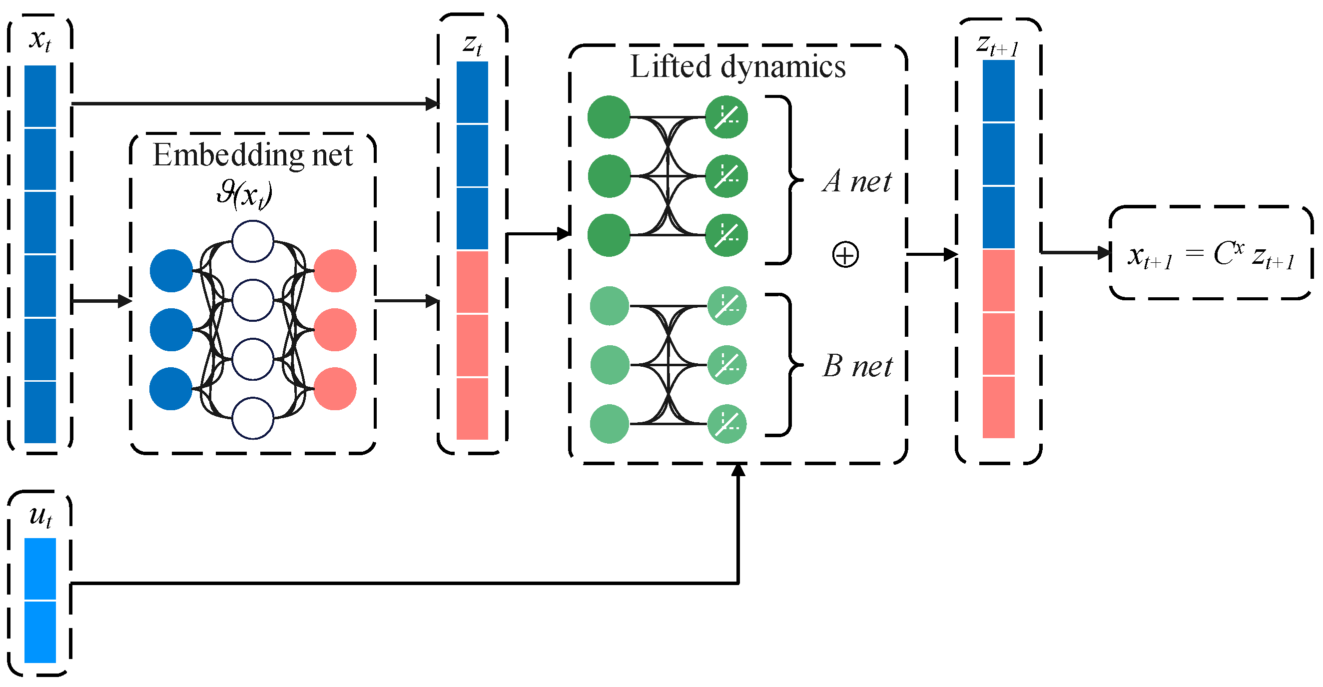
4.4. Koopman Operator

A DNN is used to parametrize the observable functions $\mathit{\psi }$ jointly with the Koopman dynamics $A\mathrm{and}B$. To this end, the following loss function is defined:

$$\begin{array}{cc}\hfill \mathcal{L}& ={\mathcal{L}}_{pred}+\alpha {\mathcal{L}}_{lin}+\beta {\mathcal{L}}_{L1}\hfill \end{array}$$

(7a)

$$\begin{array}{cc}\hfill {\mathcal{L}}_{pred}& ={\Vert x_{t+1}-C^x{\widehat{z}}_{t+1}\Vert }^2\hfill \end{array}$$

(7b)

$$\begin{array}{cc}\hfill {\mathcal{L}}_{lin}& ={\Vert z_{t+1}-{\widehat{z}}_{t+1}\Vert }^2\hfill \end{array}$$

(7c)

$$\begin{array}{cc}\hfill {\mathcal{L}}_{L1}& =\Vert A_1\Vert +\Vert B_1\Vert \hfill \end{array}$$

(7d)

The matrices A and B are parameterized by a one-layer linear NN with no bias. ${\Vert .\Vert }^2$ is the MSE, averaged over the state dimension and then over data points, and ${\widehat{z}}_t$ is the estimated value from (4) when the linear model (KL) is used or from (5) when the bilinear model (KB) is used. The hyperparameters $\alpha$ and $\beta$ govern the weight of ${\mathcal{L}}_{lin}$ and ${\mathcal{L}}_{L1}$ with respect to the prediction loss ${\mathcal{L}}_{pred}$. The loss function in (7a) is composed of three components, each corresponding to a distinct optimization objective:

• State prediction ${\mathcal{L}}_{pred}$ (7b) ensures that the Koopman dynamical system remains consistent with the original nonlinear system as it evolves over time by considering the MSE of the one-step prediction ${\widehat{x}}_{t+1}=C^x{\widehat{z}}_{t+1}$ and the actual value $x_{t+1}$.
• Linear dynamics ${\mathcal{L}}_{lin}$ (7c) corresponds to the MSE of one-step prediction error in the lifted space, ensuring that the predicted value ${\widehat{z}}_{t+1}$ matches the actual $z_{t+1}={[x_{t+1}^T,\vartheta \left(x_{t+1}\right)]}^T$.
• $L_1$ norm ${\mathcal{L}}_{L1}$ (7d) promotes the sparsity of the Koopman dynamical system and its observer, which encourages good generalization and reduces overfitting.

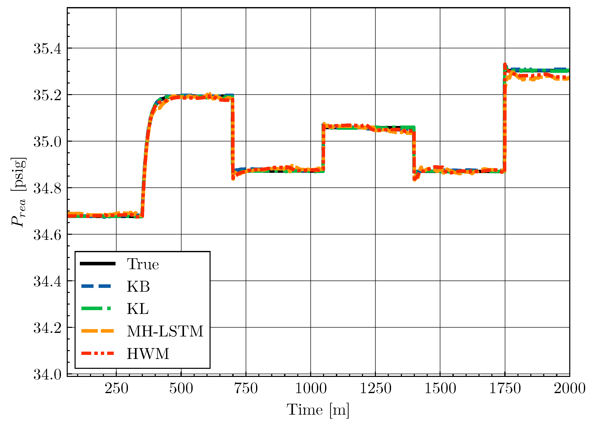
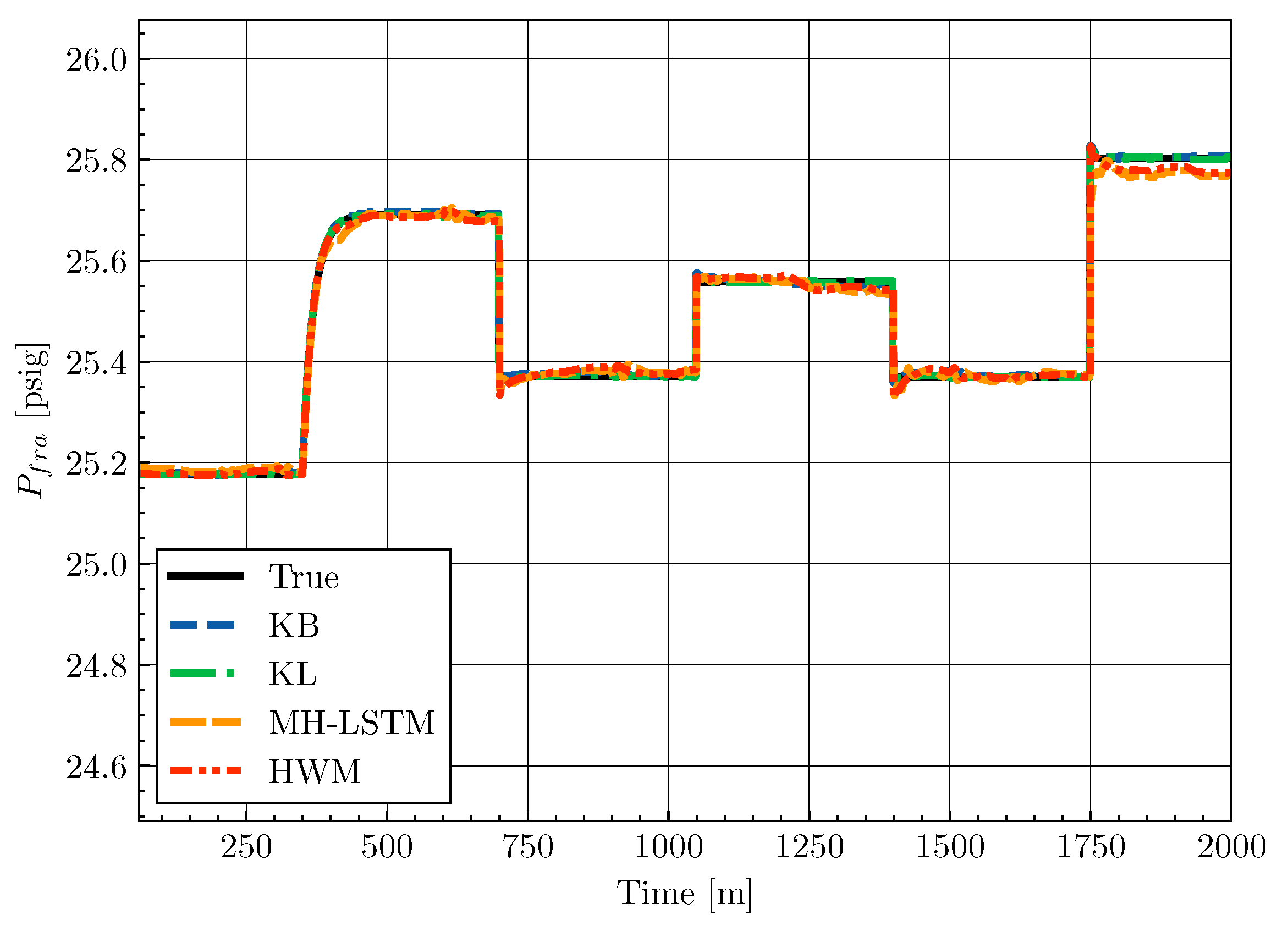
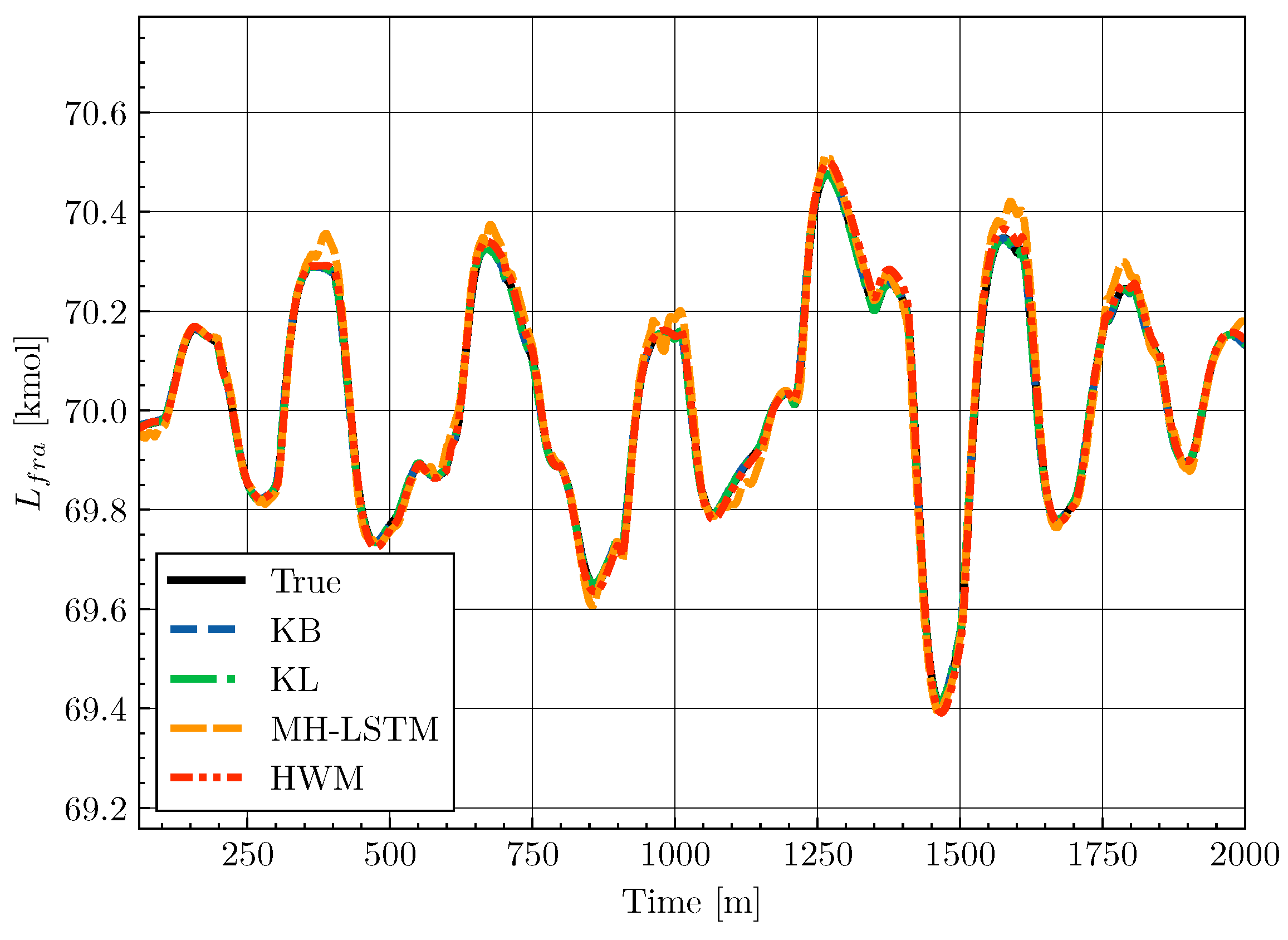
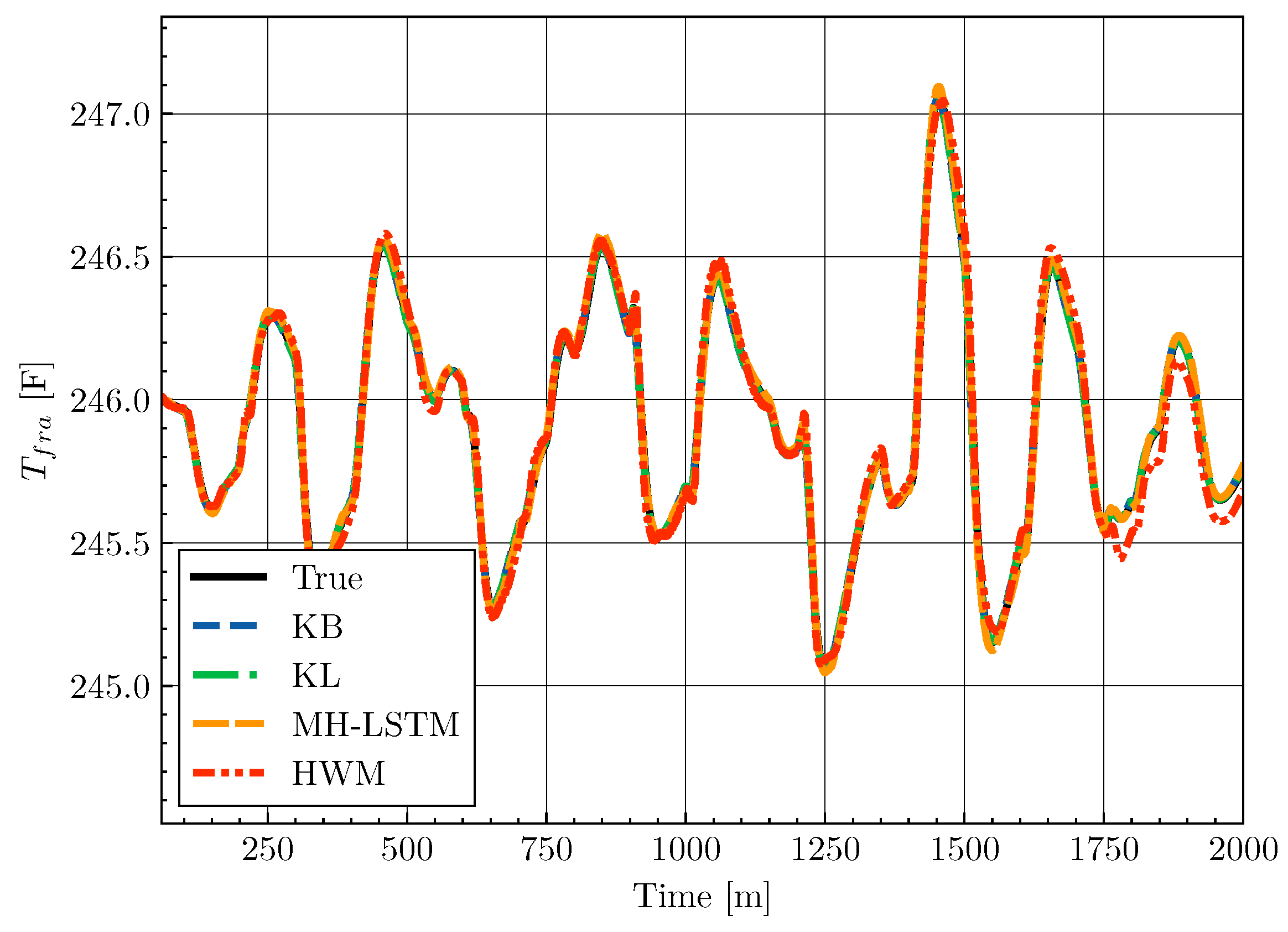
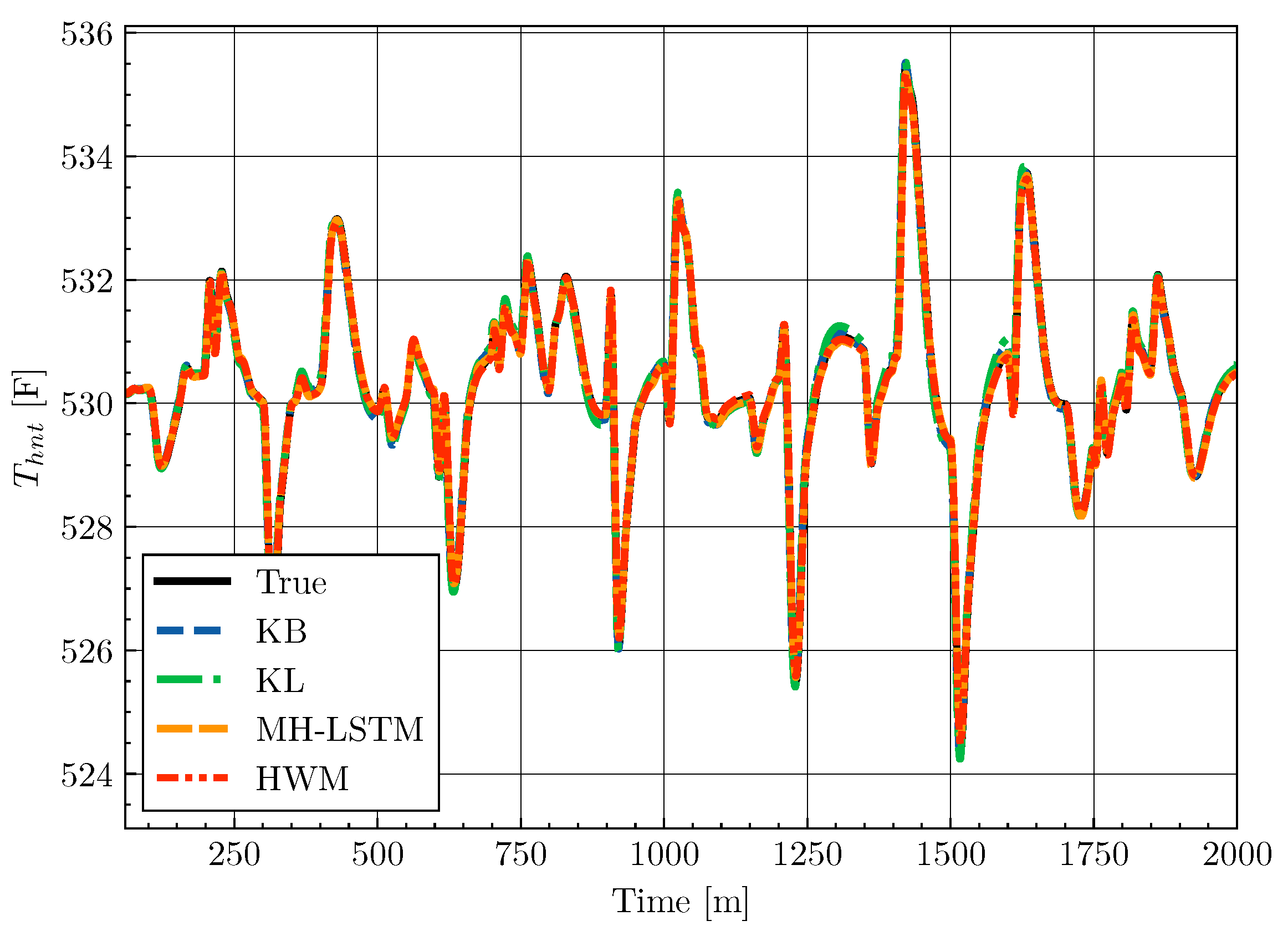
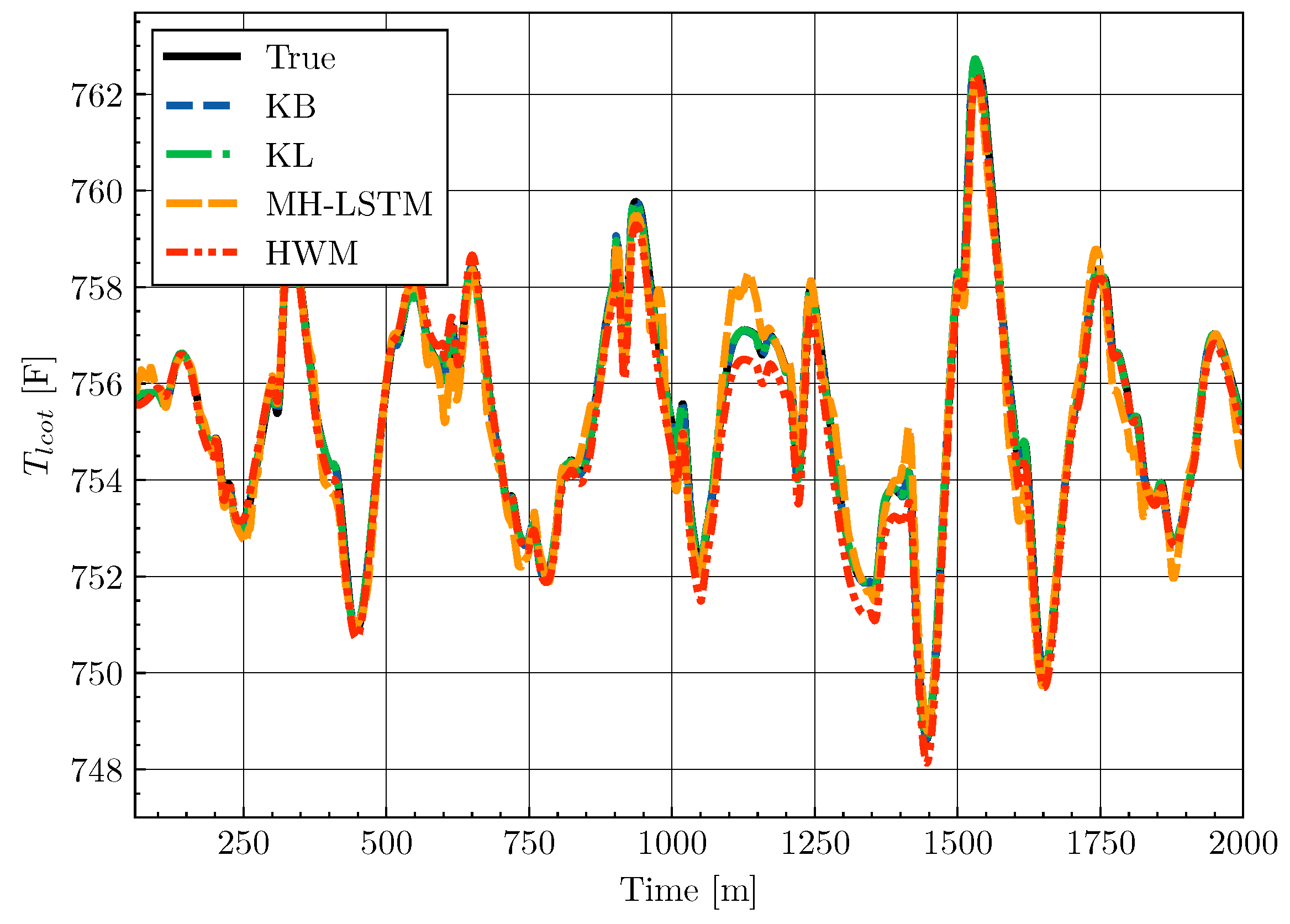
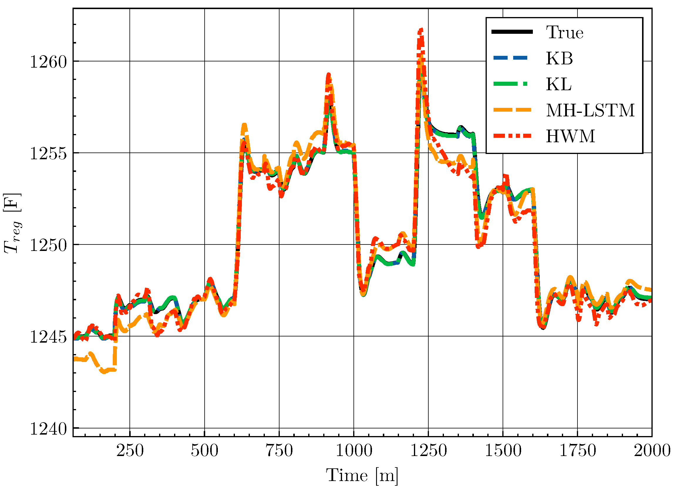
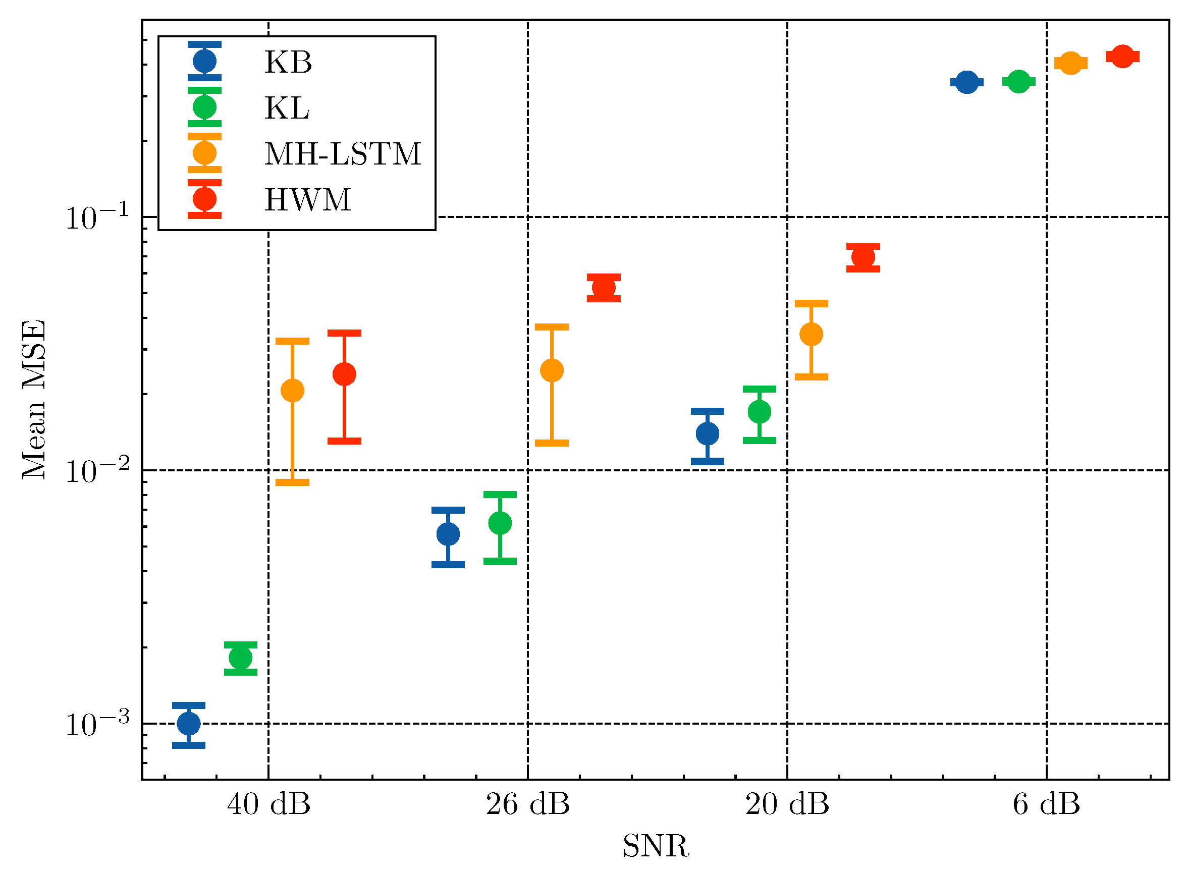
A graphical representation of the proposed DNN-KO is presented in Figure 5.

4.5. Results

The performance of each model on the test dataset is summarized in

Table 4. Average MSE for each model.

Model	Average MSE ($\times {10}^{-3}$)
KB	4.067
KL	4.673
MH-LSTM	8.171
HWM	9.556

, with detailed results for each state in Figure 6. Additionally,

Table 5. Comparison of training time and total parameters for each model.

Model	Training Time (min)	Total Params
KB	99.47	32208
KL	155.75	2875
MH-LSTM	164.90	25520
HWM	168.80	5662

presents a comparison of training time and total model parameters, offering insights into the computational requirements.

Among the four models and across all the FCC states, KB achieves the lowest MSE $4.067\times {10}^{-3}$, slightly outperforming KL, which obtains an MSE of $4.673\times {10}^{-3}$. This result aligns with expectations, as bilinear models generally exhibit higher accuracy, particularly in high-dimensional lifted dynamics [115]. The coupling of states with the inputs through the bilinear terms enables the model to capture the nonlinearities present in the FCC process more effectively, leading to reduced training time (99.47 min) compared with KL (155.75 min), despite KB having a greater number of parameters. Both KB and KL consistently outperform MH-LSTM (MSE $8.171\times {10}^{-3}$) and HW (MSE $9.556\times {10}^{-3}$) in predictive accuracy across all FCC process states.

The analysis based on the results presented in Figure 6 reveals a marked variation in MSE across the FCC states, reflecting the inherent coupling between process variables and the strong nonlinearities. For reactor temperature $T_{rea}$, the KB and KL models achieve the lowest MSE values— $2.15\times {10}^{-2}$ and $2.22\times {10}^{-2}$, respectively —highlighting their ability to capture the nonlinear reactor temperature dynamics driven by endothermic cracking reactions. Conversely, the HWM produces a substantially higher MSE of $3.17\times {10}^{-2}$, which is mainly due to the lack of sufficient state-coupling capability, limiting its accuracy in predicting complex heat transfer and reaction phenomena. The predicted results compared with the true values are shown in Figure 7. Similarly, for regenerator temperature $T_{reg}$, the KB and KL models again outperform both MH-LSTM and HWM. Specifically, the KB model attains an MSE of $7.21\times {10}^{-4}$ and the KL model one of $1.359\times {10}^{-3}$, compared with the $6.897\times {10}^{-3}$ of MH-LSTM and the $1.247\times {10}^{-2}$ of HW. This demonstrates the KB and KL models’ superior ability to represent exothermic combustion reactions and their sensitivity to variations in airflow and coke content. Comparisons between predicted and actual values for $T_{reg}$ are depicted in Figure 8.

Pressure states $P_{rea}$ and $P_{reg}$ directly influence reaction equilibria, reaction rates, and separation efficiency. All models achieve competitive performance in predicting these states, as illustrated in Figure A2 for $P_{rea}$ and Figure A4 for $P_{reg}$. Catalyst inventories $L_{rea}$ and $L_{reg}$ significantly affect residence time, reaction conversion, and energy balances. Higher MSE values for HW ($1.254\times {10}^{-2},8.676\times {10}^{-3}$) and MH-LSTM ($1.331\times {10}^{-2},9.861\times {10}^{-3}$) indicate their difficulty in capturing solid–gas interactions and mass transfer dynamics: the HWM’s limited state-coupling capability restricts its predictive accuracy, while MH-LSTM’s sequence-to-sequence architecture hinders its ability to integrate information from different process heads. In contrast, the KB and KL models consistently provide lower and competitive MSE values. The prediction versus actual values for these catalyst inventories are presented in Figure A3 and Figure A5. Similar patterns can be observed for the fractionator states $P_{fra}$, $L_{fra}$, and $T_{fra}$, as illustrated by the predictions shown in Figure A6, Figure A7 and Figure A8. A similar analysis can be performed for the remaining process states $T_{hnt}$, $T_{lcot}$, and $T_{pre}$, with prediction results shown in Figure A1, Figure A9 and Figure A10.

The sensitivity of each model was analyzed and validated under varying noise conditions. A new collection of 25 datasets was generated, each spanning a three-day operational period. Every dataset was subjected to 100 Monte Carlo evaluations at each of four SNR levels (40, 26, 20, and 6 dB), yielding 2500 trials per SNR value. For each trial, new random noise at the target SNR was added to the test inputs and outputs, inference was run, and the resulting MSE was recorded. Figure 9 presents the mean MSE and the corresponding Standard Deviation (Std Dev) error bars for the KB, KL, HW, and MH-LSTM models evaluated for each SNR level. As the noise power increases, the accuracy of each model tends to degrade, similar to any other data-driven method; however, the degree of variation changes significantly among models. The KB model outperforms all others in both accuracy (the lowest MSE) and consistency (the lowest Std Dev) across all noise levels, followed closely by KL. In contrast, the HWM and MH-LSTM demonstrate higher error rates with greater Std Dev. Practically, a higher Std Dev indicates that a model may produce erratic, inconsistent outputs, undermining overall reliability.

5. Conclusions

This paper provides a comprehensive review of current data-driven modeling methods for chemical reactors, with a particular focus on block-oriented and Koopman operator-based approaches. The advantages and limitations of these methods are examined in the context of practical implementation and control challenges. In addition, an extensive benchmark study was conducted by comparing a Deep Neural Network-based Koopman operator implemented in two forms, linear (KL) and bilinear (KB); a Multi-Input Single-Output (MISO) Hammerstein–Wiener model (HWM); and a deep Multi-Headed Long Short-Term Memory (MH-LSTM) network. Monte Carlo simulations were conducted across varying signal-to-noise ratios (SNRs) to validate the results. The KB model consistently achieved the lowest mean squared error (MSE) and Standard Deviation, demonstrating superior accuracy and robustness. The KL model followed closely, while the HWM and MH-LSTM showed higher error rates.

Block-oriented methods suffer from limited capability to capture strongly coupled Multi-Input Multi-Output nonlinear systems. Although the works in [37,54,56] attempt to address this issue, they remain restricted to certain types of input–output nonlinearities, rely on strong assumptions about input excitation, and often require the underlying system to be decomposable into separate SISO subsystems—a condition that may not hold in practice [45]. Furthermore, few studies guarantee closed-loop stability when block-oriented models are used in adaptive, robust, or real-time control applications, and their applications remain limited low-order or academic test systems. Scaling these models to large-scale, multi-variable, or time-varying nonlinear systems remains a significant challenge. Additionally, future research should prioritize the development of computationally efficient online algorithms with formal stability and convergence guarantees. In parallel, data-driven and AI-enhanced techniques offer new opportunities to advance control strategies and overcome current limitations. Additionally, hybrid identification frameworks that integrate physics-informed models, deep learning, and gray-box representations should be explored to enhance model interpretability and estimate unknown static nonlinearities or latent dynamics.

In parallel, Koopman-based methods, with robust and adaptive Koopman-based MPC, have not been extensively studied, and their implementation in large-scale industrial processes has received limited attention. Future efforts should consider probabilistic Koopman models and AI-based adaptive Koopman updates for systems with dynamics that evolve over time or are subject to noise and uncertainty. Additionally, the integration of fractional-order control techniques and active disturbance rejection within the Koopman-based framework is largely unexplored. Studies on EMPC and demand response emphasize the potential for broader, integrated objectives—such as energy efficiency and carbon footprint reduction—encouraging the extension of Koopman-based control beyond traditional regulatory tasks. There is also a need to extend Koopman methods to hybrid and mode-switching process systems, such as batch and semi-batch reactors, where dynamics change due to operating mode transitions or discrete events. For large-scale industrial plants and multi-unit operations, developing distributed Koopman-based modeling and control architectures is critical. This includes decomposing large systems into interconnected subsystems, each with its own Koopman model, and coordinating them via distributed optimization or cooperative MPC frameworks.

References

1. Harriott, P. Chemical Reactor Design; Chemical Industries, Dekker: New York, NY, USA; Basel, Switzerland, 2003. [Google Scholar]
2. Coker, A.K. Modeling of Chemical Kinetics and Reactor Design; Gulf Professional Pub.: Boston, MA, USA, 2001. [Google Scholar]
3. Dixon, A.G.; Partopour, B. Annual review of chemical and biomolecular engineering computational fluid dynamics for fixed bed reactor design. Annu. Rev. Chem. Biomol. Eng. 2020, 11, 109–130. [Google Scholar] [CrossRef] [PubMed]
4. Kataria, P.; Nandong, J.; Yeo, W.S. Reactor design and control aspects for Chemical Looping Hydrogen Production: A review. In Proceedings of the 2022 International Conference on Green Energy, Computing and Sustainable Technology (GECOST), Miri Sarawak, Malaysia, 26–28 October 2022; pp. 208–214. [Google Scholar] [CrossRef]
5. Zhang, Y.; Tiňo, P.; Leonardis, A.; Tang, K. A Survey on Neural Network Interpretability. IEEE Trans. Emerg. Top. Comput. Intell. 2021, 5, 726–742. [Google Scholar] [CrossRef]
6. Smys, S.; Zong Chen, J.I.; Shakya, S. Survey on Neural Network Architectures with Deep Learning. J. Soft Comput. Paradig. 2020, 2, 186–194. [Google Scholar] [CrossRef]
7. Khaldi, M.K.; Al-Dhaifallah, M.; Taha, O. Artificial intelligence perspectives: A systematic literature review on modeling, control, and optimization of fluid catalytic cracking. Alex. Eng. J. 2023, 80, 294–314. [Google Scholar] [CrossRef]
8. Schoukens, M.; Tiels, K. Identification of block-oriented nonlinear systems starting from linear approximations: A survey. Automatica 2017, 85, 272–292. [Google Scholar] [CrossRef]
9. Quaranta, G.; Lacarbonara, W.; Masri, S.F. A review on computational intelligence for identification of nonlinear dynamical systems. Nonlinear Dyn. 2020, 99, 1709–1761. [Google Scholar] [CrossRef]
10. Xavier, J.; Patnaik, S.K.; Panda, R.C. Process Modeling, Identification Methods, and Control Schemes for Nonlinear Physical Systems—A Comprehensive Review. ChemBioEng Rev. 2021, 8, 392–412. [Google Scholar] [CrossRef]
11. Koopman, B.O. Hamiltonian Systems and Transformation in Hilbert Space. Proc. Natl. Acad. Sci. USA 1931, 17, 315–318. [Google Scholar] [CrossRef]
12. Koopman, B.O.; Neumann, J.V. Dynamical Systems of Continuous Spectra. Proc. Natl. Acad. Sci. USA 1932, 18, 255–263. [Google Scholar] [CrossRef]
13. Mezić, I.; Banaszuk, A. Comparison of systems with complex behavior. Phys. D Nonlinear Phenom. 2004, 197, 101–133. [Google Scholar] [CrossRef]
14. Mezić, I. Spectral Properties of Dynamical Systems, Model Reduction and Decompositions. Nonlinear Dyn. 2005, 41, 309–325. [Google Scholar] [CrossRef]
15. Korda, M.; Mezić, I. Linear predictors for nonlinear dynamical systems: Koopman operator meets model predictive control. Automatica 2018, 93, 149–160. [Google Scholar] [CrossRef]
16. Bevanda, P.; Sosnowski, S.; Hirche, S. Koopman operator dynamical models: Learning, analysis and control. Annu. Rev. Control 2021, 52, 197–212. [Google Scholar] [CrossRef]
17. Otto, S.E.; Rowley, C.W. Koopman operators for estimation and control of dynamical systems. Annu. Rev. Control Robot. Auton. Syst. 2021, 4, 59–87. [Google Scholar] [CrossRef]
18. Susuki, Y.; Mezic, I.; Raak, F.; Hikihara, T. Applied Koopman operator theory for power systems technology. Nonlinear Theory Appl. IEICE 2016, 7, 430–459. [Google Scholar] [CrossRef]
19. Manzoor, W.A.; Rawashdeh, S.; Mohammadi, A. Vehicular applications of koopman operator theory—A survey. IEEE Access 2023, 11, 25917–25931. [Google Scholar] [CrossRef]
20. Shi, L.; Liu, Z.; Karydis, K. Koopman operators for modeling and control of soft robotics. Curr. Robot. Rep. 2023, 4, 23–31. [Google Scholar] [CrossRef]
21. Shi, L.; Haseli, M.; Mamakoukas, G.; Bruder, D.; Abraham, I.; Murphey, T.; Cortes, J.; Karydis, K. Koopman operators in robot learning. arXiv 2024, arXiv:2408.04200. [Google Scholar]
22. Klus, S.; Conrad, N.D. Dynamical systems and complex networks: A Koopman operator perspective. J. Phys. Complex. 2024, 5, 041001. [Google Scholar] [CrossRef]
23. Li, X.; Yan, M.; Zhang, X.; Han, M.; Law, A.W.K.; Yin, X. Efficient data-driven predictive control of nonlinear systems: A review and perspectives. Digit. Chem. Eng. 2025, 14, 100219. [Google Scholar] [CrossRef]
24. Chen, W.; Zhang, R.; Liu, H.; Xie, X.; Yan, L. A novel method for solar panel temperature determination based on a wavelet neural network and Hammerstein-Wiener model. Adv. Space Res. 2020, 66, 2035–2046. [Google Scholar] [CrossRef]
25. Esmaeilani, L.; Ghaisari, J.; Bagherzadeh, M.A. Hammerstein–Wiener identification of industrial plants: A pressure control valve case study. IET Control Theory Appl. 2021, 15, 416–431. [Google Scholar] [CrossRef]
26. Abouda, S.E.; Abid, D.B.H.; Elloumi, M.; Koubaa, Y.; Chaari, A. Identification of non-linear stochastic systems using a new Hammerstein-Wiener neural network: A simulation study through a non-linear hydraulic process. Int. J. Comput. Appl. Technol. 2020, 63, 241–256. [Google Scholar] [CrossRef]
27. Abdelsamad, A.S.; Myrzik, J.M.A.; Kaufhold, E.; Meyer, J.; Schegner, P. Voltage-Source Converter Harmonic Characteristic Modeling Using Hammerstein–Wiener Approach. IEEE Can. J. Electr. Comput. Eng. 2021, 44, 402–410. [Google Scholar] [CrossRef]
28. Micev, M.; Ćalasan, M.; Radulović, M. Identification of nonlinear Hammerstein-Wiener model for representing a field voltage-terminal voltage relation of synchronous generator. In Proceedings of the 2022 26th International Conference on Information Technology (IT), Zabljak, Montenegro, 16–19 February 2022; pp. 1–4. [Google Scholar] [CrossRef]
29. Khalfi, J.; Boumaaz, N.; Soulmani, A.; Laadissi, E.M. Nonlinear Modeling of Lithium-Ion Battery Cells for Electric Vehicles using a Hammerstein–Wiener Model. J. Electr. Eng. Technol. 2021, 16, 659–669. [Google Scholar] [CrossRef]
30. Jui, J.J.; Suid, M.H.; Musa, Z.; Ahmad, M.A. Identification of Liquid Slosh Behavior Using Continuous-Time Hammerstein Model Based Sine Cosine Algorithm. In Proceedings of the 11th National Technical Seminar on Unmanned System Technology 2019; Md Zain, Z., Ahmad, H., Pebrianti, D., Mustafa, M., Abdullah, N.R.H., Samad, R., Mat Noh, M., Eds.; Springer Nature: Singapore, 2021; pp. 345–356. [Google Scholar]
31. Spinosa, A.G.; Buscarino, A.; Fortuna, L.; Iafrati, M.; Mazzitelli, G. Data-driven order reduction in Hammerstein–Wiener models of plasma dynamics. Eng. Appl. Artif. Intell. 2021, 100, 104180. [Google Scholar] [CrossRef]
32. Abdullahi, S.B.; Ibrahim, A.H.; Abubakar, A.B. Optimizing Hammerstein-Wiener Model for Forecasting Confirmed Cases of Covid-19. IAENG Int. J. Appl. Math. 2022, 52, 22. [Google Scholar]
33. Chen, X.; Rajan, D.; Quek, C. A Deep Hybrid Fuzzy Neural Hammerstein-Wiener Network for Stock Price Prediction. In Proceedings of the 2020 International Conference on Artificial Intelligence in Information and Communication (ICAIIC), Fukuoka, Japan, 19–21 February 2020; pp. 288–293. [Google Scholar] [CrossRef]
34. Ehrmann, H. Nichtlineare Integralgleichungen vom Hammersteinschen Typ. Math. Z. 1963, 82, 403–412. [Google Scholar] [CrossRef]
35. Wiener, N.; Teichmann, T. Nonlinear Problems in Random Theory. Phys. Today 1959, 12, 52–54. [Google Scholar] [CrossRef]
36. Harnischmacher, G.; Kahrs, O.; Marquardt, W. Identification of a fluid catalytic cracking unit by means of a new multi-variable hammerstein model. IFAC Proc. Vol. 2006, 39, 672–677. [Google Scholar] [CrossRef]
37. Harnischmacher, G.; Marquardt, W. A multi-variate Hammerstein model for processes with input directionality. J. Process Control 2007, 17, 539–550. [Google Scholar] [CrossRef]
38. Harnischmacher, G.; Marquardt, W. Nonlinear model predictive control of multivariable processes using block-structured models. Control Eng. Pract. 2007, 15, 1238–1256. [Google Scholar] [CrossRef]
39. Naeem, O.; Huesman, A. Non-linear model approximation and reduction by new input-state Hammerstein block structure. Comput. Chem. Eng. 2011, 35, 758–773. [Google Scholar] [CrossRef]
40. Sudibyo; Murat, M.N.; Aziz, N. Development of multi variable neural hammerstein model for MTBE catalytic distillation. In Proceedings of the 2013 International Conference on Robotics, Biomimetics, Intelligent Computational Systems, Jogjakarta, Indonesia, 25–27 November 2013; pp. 99–103. [Google Scholar] [CrossRef]
41. Salhi, H.; Kamoun, S. A recursive parametric estimation algorithm of multivariable nonlinear systems described by Hammerstein mathematical models. Appl. Math. Model. 2015, 39, 4951–4962. [Google Scholar] [CrossRef]
42. Li, Z.; Zhu, L.; Chung, C.W.; Chen, J. Recursive identification of kernel-based hammerstein model for online energy efficiency estimation of large-scale chemical plants. Energy 2024, 309, 132946. [Google Scholar] [CrossRef]
43. Zhang, L.; Jin, D.; Zhao, J. An improved Hammerstein system identification method using Stein Variational Inference and sampling technology. J. Process Control 2023, 124, 25–35. [Google Scholar] [CrossRef]
44. Zhang, J.; Chin, K.S.; Ławryńczuk, M. Nonlinear model predictive control based on piecewise linear Hammerstein models. Nonlinear Dyn. 2018, 92, 1001–1021. [Google Scholar] [CrossRef]
45. Du, J.; Zhang, L.; Chen, J.; Li, J.; Jiang, X.; Zhu, C. Self-adjusted decomposition for multi-model predictive control of Hammerstein systems based on included angle. ISA Trans. 2020, 103, 19–27. [Google Scholar] [CrossRef] [PubMed]
46. Delou, P.d.A.; Curvelo, R.; de Souza, M.B.; Secchi, A.R. Steady-state real-time optimization using transient measurements in the absence of a dynamic mechanistic model: A framework of HRTO integrated with Adaptive Self-Optimizing IHMPC. J. Process Control 2021, 106, 1–19. [Google Scholar] [CrossRef]
47. Naregalkar, A.; Durairaj, S. A novel LSSVM-L Hammerstein model structure for system identification and nonlinear model predictive control of CSTR servo and regulatory control. Chem. Prod. Process Model. 2022, 17, 619–635. [Google Scholar] [CrossRef]
48. Demuner, R.B.; Delou, P.d.A.; Secchi, A.R. Tracking necessary condition of optimality by a data-driven solution combining steady-state and transient data. J. Process Control 2022, 118, 37–54. [Google Scholar] [CrossRef]
49. Zhang, H.; Fang, J.; Yu, H.; Guo, H.; Zhang, H. Second-order adaptive robust control of proportional pressure-reducing valves using phenomenological model. Trans. Inst. Meas. Control 2024, 46, 2367–2377. [Google Scholar] [CrossRef]
50. Mehmood, A.; Raja, M.A.Z.; Ninness, B. Design of fractional-order hammerstein control auto-regressive model for heat exchanger system identification: Treatise on fuzzy-evolutionary computing. Chaos Solitons Fractals 2024, 181, 114644. [Google Scholar] [CrossRef]
51. Qian, Z.; Hongwei, W.; Chunlei, L.; Yi, A. Establishment and identification of MIMO fractional Hammerstein model with colored noise for PEMFC system. Chaos Solitons Fractals 2024, 180, 114502. [Google Scholar] [CrossRef]
52. Arefi, M.M.; Montazeri, A.; Poshtan, J.; Jahed-Motlagh, M. Wiener-neural identification and predictive control of a more realistic plug-flow tubular reactor. Chem. Eng. J. 2008, 138, 274–282. [Google Scholar] [CrossRef]
53. Shafiee, G.; Arefi, M.; Jahed-Motlagh, M.; Jalali, A. Nonlinear predictive control of a polymerization reactor based on piecewise linear Wiener model. Chem. Eng. J. 2008, 143, 282–292. [Google Scholar] [CrossRef]
54. Oblak, S.; Škrjanc, I. Continuous-time Wiener-model predictive control of a pH process based on a PWL approximation. Chem. Eng. Sci. 2010, 65, 1720–1728. [Google Scholar] [CrossRef]
55. Abouzlam, M.; Ouvrard, R.; Mehdi, D.; Pontlevoy, F.; Gombert, B.; Vel Leitner, N.K.; Boukari, S.O. Identification of a wastewater treatment reactor by catalytic ozonation. IFAC Proc. Vol. 2012, 45, 1448–1453. [Google Scholar] [CrossRef]
56. Li, S.; Li, Y. Model predictive control of an intensified continuous reactor using a neural network Wiener model. Neurocomputing 2016, 185, 93–104. [Google Scholar] [CrossRef]
57. Yuan, P.; Zhang, B.; Mao, Z. A self-tuning control method for Wiener nonlinear systems and its application to process control problems. Chin. J. Chem. Eng. 2017, 25, 193–201. [Google Scholar] [CrossRef]
58. Peng, J.; Dubay, R.; Hernandez, J.M.; Abu-Ayyad, M. A Wiener Neural Network-Based Identification and Adaptive Generalized Predictive Control for Nonlinear SISO Systems. Ind. Eng. Chem. Res. 2011, 50, 7388–7397. [Google Scholar] [CrossRef]
59. Fu, Y.; Chai, T. Indirect self-tuning control using multiple models for non-affine nonlinear systems. Int. J. Control 2011, 84, 1031–1040. [Google Scholar] [CrossRef]
60. Tsay, C.; Kumar, A.; Flores-Cerrillo, J.; Baldea, M. Optimal demand response scheduling of an industrial air separation unit using data-driven dynamic models. Comput. Chem. Eng. 2019, 126, 22–34. [Google Scholar] [CrossRef]
61. Cai, H.; Li, P.; Su, C.; Cao, J. Double-layered nonlinear model predictive control based on Hammerstein–Wiener model with disturbance rejection. Meas. Control 2018, 51, 260–275. [Google Scholar] [CrossRef]
62. Patel, J.M.; Kumar, K.; Patwardhan, S.C. Development of Wiener-Hammerstein Models Parameterized using Orthonormal Basis Filters and Deep Neural Network. IFAC-PapersOnLine 2022, 55, 94–99. [Google Scholar] [CrossRef]
63. Kumar, K.; Patwardhan, S.C.; Noronha, S. Development of adaptive dual predictive control schemes based on Wiener–Hammerstein models. J. Process Control 2022, 119, 68–85. [Google Scholar] [CrossRef]
64. Wang, Z.; Georgakis, C. Identification of Hammerstein-Weiner models for nonlinear MPC from infrequent measurements in batch processes. J. Process Control 2019, 82, 58–69. [Google Scholar] [CrossRef]
65. Rumbo Morales, J.Y.; Brizuela Mendoza, J.A.; Ortiz Torres, G.; Sorcia Vázquez, F.d.J.; Rojas, A.C.; Pérez Vidal, A.F. Fault-Tolerant Control implemented to Hammerstein–Wiener model: Application to Bio-ethanol dehydration. Fuel 2022, 308, 121836. [Google Scholar] [CrossRef]
66. Rumbo-Morales, J.Y.; Ortiz-Torres, G.; Sarmiento-Bustos, E.; Rosales, A.M.; Calixto-Rodriguez, M.; Sorcia-Vázquez, F.D.; Pérez-Vidal, A.F.; Rodríguez-Cerda, J.C. Purification and production of bio-ethanol through the control of a pressure swing adsorption plant. Energy 2024, 288, 129853. [Google Scholar] [CrossRef]
67. Zhang, J.; Tang, Z.; Xie, Y.; Li, F.; Ai, M.; Zhang, G.; Gui, W. Disturbance-Encoding-Based Neural Hammerstein–Wiener Model for Industrial Process Predictive Control. IEEE Trans. Syst. Man Cybern. Syst. 2022, 52, 606–617. [Google Scholar] [CrossRef]
68. Jespersen, S.; Kashani, M.; Yang, Z. Hammerstein-Wiener Model Identification Of De-Oiling Hydrocyclone Separation Efficiency. In Proceedings of the 2023 9th International Conference on Control, Decision and Information Technologies (CoDIT), Rome, Italy, 3–6 July 2023; pp. 2508–2513. [Google Scholar] [CrossRef]
69. Li, J.; Zong, T.; Lu, G. Parameter identification of Hammerstein-Wiener nonlinear systems with unknown time delay based on the linear variable weight particle swarm optimization. ISA Trans. 2022, 120, 89–98. [Google Scholar] [CrossRef]
70. Dellnitz, M.; Froyland, G.; Junge, O. The Algorithms Behind GAIO-Set Oriented Numerical Methods for Dynamical Systems; Springer: Berlin/Heidelberg, Germany, 2001; pp. 145–174. [Google Scholar]
71. Carleman, T. La théorie des équations intégrales singulières et ses applications. Annales de l’institut Henri Poincaré 1930, 1, 401–430. [Google Scholar]
72. Brunton, S.L.; Budišić, M.; Kaiser, E.; Kutz, J.N. Modern Koopman Theory for Dynamical Systems. SIAM Rev. 2022, 64, 229–340. [Google Scholar] [CrossRef]
73. Goswami, D.; Paley, D.A. Global bilinearization and controllability of control-affine nonlinear systems: A Koopman spectral approach. In Proceedings of the 2017 IEEE 56th Annual Conference on Decision and Control (CDC), Melbourne, VIC, Australia, 12–15 December 2017; pp. 6107–6112. [Google Scholar] [CrossRef]
74. Garcia-Tenorio, C.; Mojica-Nava, E.; Sbarciog, M.; Wouwer, A.V. Analysis of the ROA of an anaerobic digestion process via data-driven Koopman operator. Nonlinear Eng. 2021, 10, 109–131. [Google Scholar] [CrossRef]
75. Yin, X.; Qin, Y.; Liu, J.; Huang, B. Data-driven moving horizon state estimation of nonlinear processes using Koopman operator. Chem. Eng. Res. Des. 2023, 200, 481–492. [Google Scholar] [CrossRef]
76. Narasingam, A.; Kwon, J.S.I. Koopman Lyapunov-based model predictive control of nonlinear chemical process systems. AIChE J. 2019, 65, e16743. [Google Scholar] [CrossRef]
77. Shi, Y.; Hu, X.; Zhang, Z.; Chen, Q.; Xie, L.; Su, H. Data-driven identification and fast model predictive control of the ORC waste heat recovery system by using Koopman operator. Control Eng. Pract. 2023, 141, 105679. [Google Scholar] [CrossRef]
78. Son, S.H.; Choi, H.K.; Kwon, J.S.I. Application of offset-free Koopman-based model predictive control to a batch pulp digester. AIChE J. 2021, 67, e17301. [Google Scholar] [CrossRef]
79. Son, S.H.; Narasingam, A.; Kwon, J.S.I. Development of offset-free Koopman Lyapunov-based model predictive control and mathematical analysis for zero steady-state offset condition considering influence of Lyapunov constraints on equilibrium point. J. Process Control 2022, 118, 26–36. [Google Scholar] [CrossRef]
80. Xiong, H.; Xie, L.; Hu, C.; Su, H. A fuzzy compensation-Koopman model predictive control design for pressure regulation in proten exchange membrane electrolyzer. Chin. J. Chem. Eng. 2024, 76, 251–263. [Google Scholar] [CrossRef]
81. Son, S.H.; Choi, H.K.; Moon, J.; Kwon, J.S.I. Hybrid Koopman model predictive control of nonlinear systems using multiple EDMD models: An application to a batch pulp digester with feed fluctuation. Control Eng. Pract. 2022, 118, 104956. [Google Scholar] [CrossRef]
82. Zhang, X.; Han, M.; Yin, X. Reduced-order Koopman modeling and predictive control of nonlinear processes. Comput. Chem. Eng. 2023, 179, 108440. [Google Scholar] [CrossRef]
83. Pan, C.; Li, Y. Nonlinear model predictive control of chiller plant demand response with Koopman bilinear model and Krylov-subspace model reduction. Control Eng. Pract. 2024, 147, 105936. [Google Scholar] [CrossRef]
84. Bhadriraju, B.; Narasingam, A.; Kwon, J.S.I. Machine learning-based adaptive model identification of systems: Application to a chemical process. Chem. Eng. Res. Des. 2019, 152, 372–383. [Google Scholar] [CrossRef]
85. Brunton, S.L.; Proctor, J.L.; Kutz, J.N. Discovering governing equations from data by sparse identification of nonlinear dynamical systems. Proc. Natl. Acad. Sci. USA 2016, 113, 3932–3937. [Google Scholar] [CrossRef]
86. Shi, Y.; Zhang, Z.; Chen, X.; Xie, L.; Liu, X.; Su, H. Data-Driven model identification and efficient MPC via quasi-linear parameter varying representation for ORC waste heat recovery system. Energy 2023, 271, 126959. [Google Scholar] [CrossRef]
87. Jensen, C.M.; Frederiksen, M.C.; Kallesøe, C.S.; Jensen, J.N.; Andersen, L.H.; Izadi-Zamanabadi, R. HAVOK Model Predictive Control for Time-Delay Systems with Applications to District Heating. IFAC-PapersOnLine 2023, 56, 2238–2243. [Google Scholar] [CrossRef]
88. Albalawi, F.; H., S.W. Koopman-Based Economic Model Predictive Control for Nonlinear Systems. In Proceedings of the 2023 9th International Conference on Control, Decision and Information Technologies (CoDIT), Rome, Italy, 3–6 July 2023; pp. 822–828. [Google Scholar] [CrossRef]
89. Ławryńczuk, M. Koopman operator-based multi-model for predictive control. Nonlinear Dyn. 2024, 112, 9955–9982. [Google Scholar] [CrossRef]
90. Yuan, J.; Zhao, S.; Yang, D.; Liu, C.; Wu, C.; Zhou, T.; Lin, S.; Zhang, Y.; Cheng, W. Koopman modeling and optimal control for microbial fed-batch fermentation with switching operators. Nonlinear Anal. Hybrid Syst. 2024, 52, 101461. [Google Scholar] [CrossRef]
91. Martí-Coll, A.; Rodríguez-Ramos, A.; Llanes-Santiago, O. An Optimization Approach to Select Koopman Observables for Data-Based Modeling Using Dynamic Mode Decomposition with Control. Processes 2025, 13, 284. [Google Scholar] [CrossRef]
92. Li, Q.; Dietrich, F.; Bollt, E.M.; Kevrekidis, I.G. Extended dynamic mode decomposition with dictionary learning: A data-driven adaptive spectral decomposition of the Koopman operator. Chaos Interdiscip. J. Nonlinear Sci. 2017, 27, 103111. [Google Scholar] [CrossRef]
93. Lusch, B.; Kutz, J.N.; Brunton, S.L. Deep learning for universal linear embeddings of nonlinear dynamics. Nat. Commun. 2018, 9, 4950. [Google Scholar] [CrossRef]
94. Eivazi, H.; Guastoni, L.; Schlatter, P.; Azizpour, H.; Vinuesa, R. Recurrent neural networks and Koopman-based frameworks for temporal predictions in a low-order model of turbulence. Int. J. Heat Fluid Flow 2021, 90, 108816. [Google Scholar] [CrossRef]
95. Maksakov, A.; Palis, S. Koopman-based data-driven control for continuous fluidized bed spray granulation. IFAC-PapersOnLine 2021, 54, 372–377. [Google Scholar] [CrossRef]
96. Schulze, J.C.; Doncevic, D.T.; Mitsos, A. Identification of MIMO Wiener-type Koopman models for data-driven model reduction using deep learning. Comput. Chem. Eng. 2022, 161, 107781. [Google Scholar] [CrossRef]
97. Ahmed, A.; del Rio-Chanona, E.A.; Mercangöz, M. Linearizing nonlinear dynamics using deep learning. Comput. Chem. Eng. 2023, 170, 108104. [Google Scholar] [CrossRef]
98. Abubakar, A.N.; Khaldi, M.K.; Aldhaifallah, M.; Patwardhan, R.; Salloum, H. Identification of Crude Distillation Unit: A Comparison between Neural Network and Koopman Operator. Algorithms 2024, 17, 368. [Google Scholar] [CrossRef]
99. Liu, Y.; Wang, S.; Xu, L. Deep Koopman-VAE Based Process Monitoring for Industrial Biosystems. In Proceedings of the 2023 IEEE 3rd International Conference on Data Science and Computer Application (ICDSCA), Dalian, China, 27–29 October 2023; pp. 252–260. [Google Scholar] [CrossRef]
100. Luo, J.; Çıtmacı, B.; Jang, J.B.; Abdullah, F.; Morales-Guio, C.G.; Christofides, P.D. Machine learning-based predictive control using on-line model linearization: Application to an experimental electrochemical reactor. Chem. Eng. Res. Des. 2023, 197, 721–737. [Google Scholar] [CrossRef]
101. Irani, F.N.; Yadegar, M.; Meskin, N. Koopman-based deep iISS bilinear parity approach for data-driven fault diagnosis: Experimental demonstration using three-tank system. Control Eng. Pract. 2024, 142, 105744. [Google Scholar] [CrossRef]
102. Li, X.; Bo, S.; Zhang, X.; Qin, Y.; Yin, X. Data-driven parallel Koopman subsystem modeling and distributed moving horizon state estimation for large-scale nonlinear processes. AIChE J. 2024, 70, e18326. [Google Scholar] [CrossRef]
103. Tian, W.; Liu, Y.; Xie, J.; Huang, W.; Chen, W.; Tao, T.; Xin, K. Simulation and Dynamic Properties Analysis of the Anaerobic-Anoxic-Oxic Process in a Wastewater Treatment PLANT Based on Koopman Operator and Deep Learning. Water 2023, 15, 1960. [Google Scholar] [CrossRef]
104. Han, M.; Yao, J.; Law, A.W.K.; Yin, X. Data-Driven Economic Predictive Control of Wastewater Treatment Process with Input-Output Koopman Operator. In Proceedings of the 2024 American Control Conference (ACC), Toronto, ON, Canada, 10–12 July 2024; pp. 3025–3030. [Google Scholar] [CrossRef]
105. Han, M.; Li, Z.; Yin, X.; Yin, X. Robust Learning and Control of Time-Delay Nonlinear Systems with Deep Recurrent Koopman Operators. IEEE Trans. Ind. Inform. 2024, 20, 4675–4684. [Google Scholar] [CrossRef]
106. Li, Z.; Han, M.; Vo, D.N.; Yin, X. Machine learning-based input-augmented Koopman modeling and predictive control of nonlinear processes. Comput. Chem. Eng. 2024, 191, 108854. [Google Scholar] [CrossRef]
107. Li, Q.; Zhang, J.; Wan, H.; Zhao, Z.; Liu, F. Physics-informed neural networks for multi-stage Koopman modeling of microbial fermentation processes. J. Process Control 2024, 143, 103315. [Google Scholar] [CrossRef]
108. Yan, M.; Han, M.; Law, A.W.K.; Yin, X. Self-tuning moving horizon estimation of nonlinear systems via physics-informed machine learning Koopman modeling. AIChE J. 2025, 71, e18649. [Google Scholar] [CrossRef]
109. Kumar, D.; Dixit, V.; Ramteke, M.; Kodamana, H. Learning Interpretable Representation of Koopman Operator for Non-linear Dynamics. In 34th European Symposium on Computer Aided Process Engineering/15th International Symposium on Process Systems Engineering; Manenti, F., Reklaitis, G.V., Eds.; Elsevier: Amsterdam, The Netherlands, 2024; Volume 53, pp. 2773–2778. [Google Scholar] [CrossRef]
110. Mayfrank, D.; Mitsos, A.; Dahmen, M. End-to-end reinforcement learning of Koopman models for economic nonlinear model predictive control. Comput. Chem. Eng. 2024, 190, 108824. [Google Scholar] [CrossRef]
111. Treese, S.A.; Pujadó, P.R.; Jones, D.S.J. (Eds.) Handbook of Petroleum Processing; Springer International Publishing: Cham, Switzerland, 2015. [Google Scholar] [CrossRef]
112. Hsu, C.S.; Robinson, P.R. Petroleum Science and Technology; Springer International Publishing: Cham, Switzerland, 2019. [Google Scholar] [CrossRef]
113. Santander, O.; Kuppuraj, V.; Harrison, C.A.; Baldea, M. An open source fluid catalytic cracker-fractionator model to support the development and benchmarking of process control, machine learning and operation strategies. Comput. Chem. Eng. 2022, 164, 107900. [Google Scholar] [CrossRef]
114. Mustapha K., K.; Mujahed, A.; Othman, T.; Mahmood, T.; Abdullah, A. Computational Modeling of FCC Unit. ASEJ, 2025; manuscript submitted for publication; currently under review. [Google Scholar]
115. Bruder, D.; Fu, X.; Vasudevan, R. Advantages of Bilinear Koopman Realizations for the Modeling and Control of Systems With Unknown Dynamics. IEEE Robot. Autom. Lett. 2021, 6, 4369–4376. [Google Scholar] [CrossRef]
Figure 1. Block-oriented structures: (a) Hammerstein model, (b) Wiener model, and (c) Hammerstein–Wiener model.
Mathematics 13 02411 g001
Figure 2. FCC fractionator process diagram.
Mathematics 13 02411 g002
Figure 3. FCC-Multi-Headed LSTM (MH-LSTM) architecture.
Mathematics 13 02411 g003
Figure 4. Multi-Input Single-Output HWM.
Mathematics 13 02411 g004
Figure 5. Deep Neural Network Koopman Operator.
Mathematics 13 02411 g005
Figure 6. MSE for each FCC state and for each model.
Mathematics 13 02411 g006
Figure 7. Comparison of predicted vs. true values of each model for Trea.
Mathematics 13 02411 g007
Figure 8. Comparison of predicted vs. true values of each model for Treg.
Mathematics 13 02411 g008
Figure 9. Average and Standard Deviation of MSE for each model across different SNR values.
Mathematics 13 02411 g009