Abstract
This article investigates the Q-Problem, a novel theoretical framework for post-quantum cryptography. It aims to redefine cryptographic hardness by moving away from problems with unique solutions toward problems that admit multiple indistinguishable preimages. This shift is motivated by the structural vulnerabilities that quantum algorithms may exploit in traditional formulations. To support this paradigm, we define new cryptographic primitives and security notions, including Q-Indistinguishability, Long-Term Secrecy, and a spectrum of Q-Secrecy levels. The methodology formalizes the Q-Problem as a system of expressions, called Q-expressions, that must satisfy a set of indistinguishability and reduction properties. We also propose a taxonomy of its models, including Connected/Disconnected, Totally/Partly, Fully/Partially Probabilistic, Perfect, and Ideal Q-Problem variants. These models illustrate the versatility across a range of cryptographic settings. By abstracting hardness through indistinguishability rather than solvability, Q-Problem offers a new direction for designing cryptographic protocols resilient to future quantum attacks. This foundational framework provides the foundations for long-term, composable, and structure-aware security in the quantum era.
Keywords:
hard mathematical problem; Information security; perfect confidentiality; post-quantum techniques; Q-Problem MSC:
68M25; 11T71; 68P25; 94A60
1. Introduction
Post-quantum cryptography seeks to develop cryptographic systems that remain secure against quantum adversaries. The advent of quantum algorithms, e.g., Shor’s algorithm for factoring and discrete logarithms and Grover’s algorithm for unstructured search [1,2], poses a significant threat to many classical cryptographic schemes [3]. In response, researchers proposed new schemes based on assumptions believed to be quantum-resistant, including lattice-based [4], code-based [5], multivariate polynomial [6], and hash-based cryptography [7].
However, a common trait shared by most post-quantum problems is that they ultimately aim to protect a unique hidden solution. This structural assumption, while seemingly harmless, may eventually be exploited by future quantum techniques. For example, in certain code-based settings, even if the decoding problem is computationally hard, the existence of a unique solution could facilitate distinguishability or targeted inversion under quantum models [5,8,9]. Thus, post-quantum security may be compromised not by current algorithms, but by structural weaknesses in the underlying problem formulations.
To address this, we propose a new theoretical direction: the Q-Problem (QP) paradigm. Rather than protecting a single solution, QP defines problems where multiple valid preimages exist for a given instance, and the true one is computationally indistinguishable from the others. The goal is to frustrate quantum search strategies not by sheer hardness, but by deliberately removing uniqueness. QP thus introduces a new class of cryptographic hardness assumptions that shift the adversary’s challenge from solving to selecting, disrupting the very structure quantum algorithms are designed to exploit.
The Q-Problem framework leads to a family of new primitives and security notions suited to long-term, post-quantum resilience. These include Q-Indistinguishability (Q-IND): a hardness notion based on indistinguishable preimage sets. LTS: a model for protecting information across decades. Q-Secrecy levels such as , quantifying degrees of entropy and indistinguishability.
Furthermore, QP enables a taxonomy of the types of theoretical problems (Table 1): connected/disconnected QP, fully/partially QP, fully/partially probabilistic QP, perfect QP, and ideal QP, allowing tailored cryptographic designs in various application scenarios [10].

Table 1.
Notations table.
In this work, we present the formal construction of the Q-Problem paradigm, exploring its theoretical foundation, key properties, and cryptographic potential. By redefining secrecy as a property of indistinguishability among many candidates, QP offers a new and complementary defense model for the quantum era, one that shifts focus from solving to surviving search. Illustrative examples of Q-expressions over various data types and operations are presented in Appendix A.4 to demonstrate the applicability of the QP framework across classical and modern digital domains.
2. Definitions
In this section, three new definitions are introduced.
2.1. Long-Term Secrecy (LTS)
We define LTS as the property whereby multiple indistinguishable solutions exist for the same system instance, such that only one corresponds to the intended (original) input. Crucially, no observer without prior knowledge can determine which preimage is correct.
Let denote the output space, the input space, and be a function. For any output , let denote the set of preimages of o. Among these, we define as the number of indistinguishable preimages of o, i.e., those that are computationally or semantically indistinct from one another in the absence of additional information.
A system satisfies LTS if the indistinguishability of these preimages persists over time and the number of such indistinguishable preimages meets the criterion shown by (1).
If for every , then f is injective, i.e., one-to-one. This means that distinct inputs always map to distinct outputs, and hence each output corresponds to a unique input. This injectivity implies the absence of ambiguity, which contradicts the notion of indistinguishability that LTS aims to guarantee. In such a case, either immediately or in the future, an adversary could potentially compute the inverse and retrieve the original input, thereby breaking the LTS of the system. Therefore, this condition serves as a security requirement; it specifies when a system can be said to satisfy LTS, rather than asserting that all systems inherently meet it.
2.2. Q-Indistinguishability Assumption (Q-IND)
Let be the set of all digital data structures, and let ⋆ be a generic operation over (Equation (2)).
Suppose an oracle samples uniformly at random and outputs . Then the Q-IND assumption states:
Given an instance and the operation ⋆, it is computationally infeasible to identify the correct input pair from the set of all uniformly distributed valid pairs satisfying , when the number of such solutions satisfies .
This assumption does not assert that computing a valid preimage is hard, but rather that distinguishing the correct preimage among uniformly distributed and computationally indistinguishable candidates is infeasible without auxiliary information.
To define the Q-IND experiment formally, let the set of all valid preimages that defined as shown in (3).
Assume that for some indistinguishability parameter I. For a quantitative interpretation of I, it could be related to a concrete security level (security parameter ), e.g., . The set of solutions () satisfying can be viewed as a structured level set in , potentially exhibiting algebraic or geometric properties depending on ⋆.
Q-IND Game can be shown as follows:
- 1.
- The challenger samples and computes .
- 2.
- The challenger computes the preimage set .
- 3.
- The index is set such that .
- 4.
- The challenger sends to the adversary .
- 5.
- The adversary outputs an index .
- 6.
- The adversary wins if .
Q-IND advantage is illustrated by (4).
The notation represents the probability that the adversary outputs the correct index , conditioned on having access to the values a and . This probability is taken over all internal randomness of both the adversary and the challenger, and the conditioning reflects the fact that the adversary’s output depends on its input view.
The index corresponds to the location of the true preimage within the preimage set . Since contains all valid input pairs such that . Hence, the number of possible values that can take is exactly . An adversary making a uniform random guess has a success probability of . This forms the basis of the Q-IND advantage definition, which captures how much better the adversary performs compared to random guessing.
Q-IND assumption is defined by (5). We say that f satisfies Q-IND assumption if, for all probabilistic polynomial adversaries , there exists a negligible function such that:
Thus, no quantum PPT adversary can do better than a negligible advantage over random guessing.
The Q-IND assumption provides a foundation for cryptographic schemes that rely on semantic ambiguity in inversion. It supports primitives where: (a) Multiple valid preimages exist for the same output. (b) Only one preimage is correct in context (e.g., authentication or identity binding). (c) An adversary cannot identify the correct preimage without additional distinguishing information. This aligns with the QP challenge and supports LTS under controlled ambiguity.
The concept of Q-Indistinguishability (Q-IND) is closely related to classical security notions such as Indistinguishability Under Chosen-Plaintext Attack (IND-CPA) and Chosen-Ciphertext Attack (IND-CCA). While IND-CPA and IND-CCA define adversarial games where the goal is to distinguish between encryptions of two chosen plaintexts, Q-IND focuses on the adversary’s inability to identify the correct preimage among many indistinguishable valid candidates that map to the same output. In a classical setting, Q-IND introduces a stronger ambiguity by eliminating the notion of a unique solution, whereas IND-CPA and CCA still assume a single encryption of a specific message. In the quantum setting, Q-IND becomes even more significant, as it assumes hardness holds even when the adversary can query the function (or oracle) in superposition. This contrasts with quantum versions of IND-CPA/CCA, where encryption or decryption oracles are adapted to handle quantum queries. Therefore, Q-IND generalizes the notion of semantic security by enforcing indistinguishability over solution spaces rather than encrypted message pairs, offering a deeper level of resistance in both classical and quantum adversarial models.
2.3. Q-Secrecy Level
Let be the hardness level to find the preimages. The first level is , it can be expressed as Easy to Find, Impossible to Distinguish (EFID). For example, is easy to resolve, i.e., to find the possible preimages, but without any additional information about , it is impossible to guess the correct pair.
The second level is ; it can be expressed as Hard to Find, Impossible to Distinguish (HFID). For example, is not easy to resolve with large ( with brute-force strategy). It is considered computationally hard, like a variant of the Diophantine problem modulo p.
The other factor of Q-Secrecy that can be integrated with is the number of solutions (# preimages), which can be referred to as the degree (Equation (6)).
where denotes the number of solutions of a single equation i, and is the number of solutions of the entire system. Thus, the first example belongs to and the second belongs to .
Supposing that , of hardness level is as follows: , (, ), then . The level between and depends on the scenario.
The hash function could be another example of HFID if the input length is large and unknown to the adversary, which will give him a large set of preimages, of course, in a context where he cannot determine which is the correct one. This example remains valid unless an efficient algorithm exists to calculate the hash preimages other than brute force, which is infeasible for large input sizes. Otherwise, it is EFID.
3. QP: Formal Presentation
QP is defined as follows:
denotes the overall system or protocol instance, e.g., , and , so must satisfy QP conditions, namely Points (1) through (6) as defined in the QP framework.
A is an abstract expression over digital structures with arbitrary operations, whose goal is to encode its operands using one or more forms of data hiding under formal indistinguishability constraints, which includes a wide spectrum of computational and information-theoretic methods; Qe could be an atomic digital object or composed with any meaningful operations between digital structures. Operands x and y may be an atomic digital object or a composed expression built from subcomponents via one or more operations, e.g., , , and so on.
In Point 2, ⊥ states that the values of and remain hidden even with combining Q-expressions.
In Point 3, ⊥ states that neither x nor y has any relation with the public parameter p that would reveal hidden values, and that the adversary cannot infer any confidential information about the secret from .
means that , it can be presented as: .
means that where : are instances. This states that combining Q-expressions gives more than two indistinguishable solutions.
Point 6 in QP definition meant that the new system derived (reduced) from combining of the initial using operations must be, in turn, a QP, and so on (Equation (7)).
For instance, we put , is QP; but , it is not QP because the secret variable x can be retrieved using a quantum computer.
To evaluate a , only hidden objects are considered, i.e., coefficients/constants are ignored. For example, are elementary (atomic).
In practice, there are some conditions that must be applied to ensure the safety of Q-IND. Operation ⋆ must be free of trapdoor patterns, e.g., for multiplication , the adversary could try all divisors of a; if any structure leaks, the assumption might fail. Side channel attacks must be taken into account; if an adversary can learn partial bits of the inputs, e.g., via timing, Q-IND can be broken. There should not be a correlation with the external state, i.e., inputs must appear random even if the adversary knows message/ciphertext mappings.
4. QP: Models, Quantitative View, and Use Cases
We define five models of QP.
4.1. Connected and Disconnected QP (CQP, DQP)
CQP, DQP are illustrated in (8)
In CQP, there exists at least one common elementary secret object shared between two or more in . Consider these examples:
Note that the parameter p is not considered a common object. Therefore, if where is public and does not contain a secret object, that does not affect the system being DQP.
4.2. Totally and Partly QP (TQP, PQP)
If CQP/DQP is about two different (vertical change and ), TQP/PQP is about the same (horizontal change and ), but two different inputs. Suppose that their corresponding outputs are (Equation (9)).
Consider this example: k is the secret key for encryption, m is the plaintext. Suppose that the input is .
In , note that m (represents y) has changed but k (represents x) does not, i.e., . Therefore, this is PQP and not TQP.
4.3. Fully and Partially Probabilistic QP (FPQP, PPQP)
If TQP/PQP is a horizontal change for two different inputs, FPQP/PPQP is a horizontal change for the same input. Suppose that the corresponding outputs are (Equation (10)).
Consider this example: k is the secret key for encryption, m is the plaintext, and r is a fresh random number. Suppose that the input is .
Note that in PPQP, where and , y has changed but x has not in the two instances and for the same input m. In contrast, in FPQP where , , both x and y have changed (, ). This scheme is similar to Gentry’s scheme, , where are random.
In deterministic QP (SQP), , the same output for the same input. For operations that are not repetitive, such as generating a public key, it is sufficient for x and y to be unknown.
We emphasize that if a system satisfies or , then it necessarily satisfies or , respectively.
4.4. Perfect QP (FQP)
An FQP is a fully probabilistic QP (FPQP) such that, under Successive Breakdown of Components (SBC), each resulting part remains an FPQP, down to the final, indivisible (elementary, atomic, or non-decomposable ).
Let be a QP expression defined as where each . As shown in (11), SBC is a recursive process that transforms into a sequence of finer-grained expressions by recursively applying structural expansions to one or more components based on their internal structure, subject to the following:
1. Initial Step: Let .
2. Recursive Step: For each , the k-th breakdown produces a new expression by replacing at least one component with a more granular expression: where each .
3. Termination Condition: The process continues until all components are elementary (atomic), meaning they are no longer decomposable within the domain .
We denote the final expression by , where ℓ is the number of breakdown steps required to reach a fully resolved form (elementary form).
In the context of Perfect QP (FQP), each intermediate expression must remain a valid FPQP throughout the SBC process.
Consider the precedent example of . If we put , , the first SBC on x gives , , which is only PPQP. Therefore, this is not FQP.
Again, consider the precedent example of , so and . Suppose now that the same plaintext m and the encryption secret key k have intervals. When calculating c, variables m and k are selected at random from their intervals. The original plaintext can be retrieved as: where ÷ denotes the integer division, is a constant secret key, and r is a random number less than . An illustrative numerical example could be: , etc., , . Then, , , and , . Subexpression y is atomic, the SBC on x is . Note that and for the same plaintext. On the other hand, each elementary Q-expression is changed for two instances of the same input. Accordingly, this scheme is .
4.5. Ideal QP (IQP)
IQP is , which means a Disconnect and a Perfect QP. An example of IQP is introduced: a Message-Fragmentation-based OTP encryption scheme (MFOTP). In this scheme, where and are two random fragments of m, even if the same plaintext m is encrypted again.
Why is the suggested MFOTP an IQP?
Let be a system, , , this is presented as . Both x and y are hidden, is satisfied due to the existence of many indistinguishable () where . Thus, is QP.
Elements x and y are atomic, and , so is DQP. For two inputs : ; and .
Noting that and , so is TQP. In addition, for a new m, a new fragmentation will be used, i.e., , and new keys are used (). Every object in is changed even with the same input; therefore, this scheme is FPQP. Now, MFOTP is DQP and FPQP, which means that MFOTP is an IQP.
4.6. OTP and Q-Problem
It is known that in OTP, a one-time encryption key is used. For example, if and for the same input m, we find that . Therefore, the basic version of OTP is not fully probabilistic but a partially probabilistic QP.
To convert it from PPQP to FPQP, random fragmentation of the message m into two parts can be used. Thus, the first encryption of m is , the second encryption of m is . That gives and , the same thing for the second part of m i.e., and . Therefore, using two keys for each message instead of one is needed. Since it is easy to obtain valid solutions () in for a given c, basic OTP and MFOTP are . Figure 1 summarizes the presented Q-Problem models.
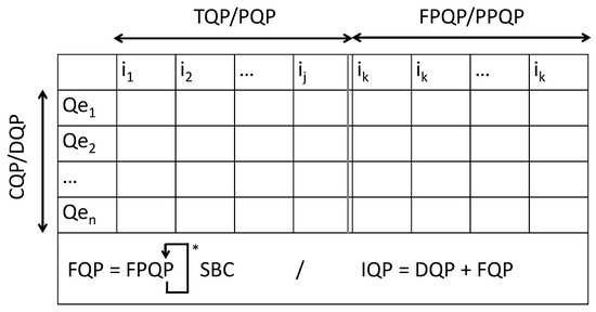
Figure 1.
Illustration of Q-Problem taxonomy, “*” indicates repeating the SBC operation.
4.7. Quantitative View of QP Models
Although the QP taxonomy is defined structurally, each class can be approximated quantitatively in terms of the number of indistinguishable preimages () and the associated adversarial advantage. For example, in an Ideal QP (IQP), each output is derived from a disconnected and perfectly decomposable expression, producing a large set of indistinguishable preimages and minimizing the adversary’s ability to recover the true origin. In contrast, classes such as PPQP or PQP may provide only partial variation or structural overlap. Table 2 summarizes the distinctions across QP levels, allowing practitioners to select appropriate configurations based on entropy goals and attack models.
Table 2.
Qualitative and quantitative comparison of QP model classes.
Table 2 shows a qualitative and quantitative comparison of QP model classes, where and are entropy estimates for indistinguishable sets, and Adv. success (respectively, ). We can not compare CQP/DQP with other classes because CQP/DQP is inter-Qe and the others are intra-Qe, except IQP, which relies on two dimensions.
4.8. QP Use Cases
This point explains how the belonging of schemes to QP is analyzed.
Let us take RSA, where e is the public key. Since values c and e are given, and the only hidden variable is m, RSA’s expression is in the form of where y is known, so has only one solution. Therefore, point 4 in the formal definition is not satisfied, and RSA is not QP. Furthermore, e depends on n where .
Let us take ElGamal, where is the public key and k is the secret key. The first part belongs to QP, (unknown) and (unknown because r is hidden). Since g is public, the expression of the second part is in the form of where x is known, so ElGamal does not belong to QP.
Let us take Gentry’s FHE scheme (DGHV) that is written as where r and q are random for each encryption and p is a secret key. It can be considered that this scheme is QP, if we put and , then , this form verifies all conditions of QP. Since it has only one , it is DQP; for two different inputs, will be changed, which makes it TQP; for two different instances of the same input, will be changed, so it is FPQP; we note that not each elementary variable, e.g., m, will be changed for two instances of the same input, so it is not FQP; consequently, the scheme is not IQP. Given c, the possible solutions in are easy to find, so Gentry’s scheme is .
As for Kyber-NIST, Key Encapsulation Mechanism, the public key is where , () is the secret key. The encapsulation function computes where are random. The system satisfies QP definition, for example, are hidden in , are hidden in , are hidden in . We note that , and , so it is not DQP but CQP. To check TQP/PQP (respectively, FPQP/PPQP, FQP), is not considered because it concerns the generation of the public key, and it is computed once. If we put (respectively, ), terms will be changed for two different inputs, so it is TQP, also for two different instances of the same inputs (new encryption of the same plaintext), so it is FPQP. Kyber is not FQP because not every elementary variable will be changed. After SBC, (or t), for two instances, does not change. Consequently, Kyber is not IQP. Given t in and in , the possible solutions are easy to find, so Kyber is .
The same thing for FrodoKEM-NIST, Key Encapsulation Mechanism, it uses the public key where , the encapsulation is: .
In Dilithium-NIST, Digital Signature Algorithm, the public key is where , () is the secret key. The signature function computes where y is random.
The system, , satisfies QP definition. We note that , and , so it is not DQP but CQP. The common variable A is not considered because it is public. In , we put ; y will not be changed for two different inputs, so the scheme is PQP, also for two different instances of the same inputs, so it is PPQP. Consequently, Dilithium is not FQP nor IQP. With given in , the possible solutions for are not easy to find, so Dilithium is .
As for McEliece-NIST public-key encryption, the public key is where , () is the secret key. The encryption function computes where e is random. The system is . We note that , so the system is not DQP but CQP. In , we put ; will be changed for two different inputs, so it is TQP, not for two different instances of the same inputs, so it is PPQP. In SBC, we put ; will not be changed for two instances of the same input, so it is not FQP; consequently, McEliece is not IQP. With a given in , the possible solutions for (S, G, P, m, e) are easy to find, so Dilithium is .
Table 3 summarizes this analysis and classification.
Table 3.
Classification of cryptographic schemes under QP. FQP is FPQP*, and IQP is DQP and FQP.
The QP framework establishes a novel structural foundation based on indistinguishability of preimages, aiming primarily to resist quantum adversaries. However, QP compliance, defined by satisfying the indistinguishability conditions such as Q-IND, does not automatically imply security against classical attacks. For instance, the expression may satisfy the QP requirement of having multiple indistinguishable pairs that map to the same ciphertext c. However, this basic scheme is vulnerable to classical attacks, such as known-plaintext or chosen-plaintext attacks, especially if the key k is reused or low-entropy inputs are involved. In such cases, an adversary can trivially recover m or k by computing modular inverses or exploiting statistical patterns. This illustrates that not every QP-compliant scheme is secure against classical threats. As in traditional cryptography, QP-based designs must be fortified with adequate primitives and resistance to adaptive attacks to achieve robust classical and quantum security. Therefore, while QP offers a strong post-quantum abstraction, practical schemes must still undergo rigorous classical cryptanalysis.
5. Conclusions
This article introduced the QP as a new theoretical framework in cryptography and privacy-preserving, centered on the definition of novel primitives and security notions such as Q-IND and LTS. The formalism captures how digital expressions can hide information structurally, across a wide class of operations and data types, by enforcing indistinguishability as a foundational property. As an initial demonstration, we focused on specific “expression forms, data structure, and operations”, illustrating the core components of the framework. While this version did not explore the full diversity of digital data structures, QP lays the groundwork for future exploration.
Although the present work focuses on classical digital structures, extending the QP framework to operate directly on quantum states, such as qubits, remains an open direction. Such an extension would require redefining Q-expressions in the context of quantum information theory and exploring indistinguishability under quantum superposition and entanglement.
Author Contributions
Conceptualization: M.K.; methodology: M.K., and M.H.; validation: M.K., M.H., and S.A.; formal analysis: M.K., and S.A.; writing—original draft preparation: M.K.; writing—review and editing: M.K., M.H., and S.A. All authors have read and agreed to the published version of the manuscript.
Funding
The study is supported by the grant no. CRPG-25-3092 under the Cybersecurity Research and Innovation Pioneers Grant, provided by the National Cybersecurity Authority NCA, in the Kingdom of Saudi Arabia.
Data Availability Statement
Data are contained within the article.
Acknowledgments
We gratefully acknowledge the support of the National Cybersecurity Authority (NCA), Kingdom of Saudi Arabia, through the Cybersecurity Research and Innovation Pioneers Grant.
Conflicts of Interest
The authors declare no conflicts of interest.
Appendix A. Digital Structures, Operations, and Examples in the QP Framework
Appendix A.1. General Forms of Quantum Expressions (QEs)
Each Q-expression is defined as a data-hiding transformation of the form , where , and ⋆ is an operation over digital structures. The design of can leverage a wide range of hiding mechanisms, generalized as follows:
- Encrypted QEs: data are transformed using a cryptographic key to ensure confidentiality.
- Obfuscated QEs: program or function logic is restructured to preserve behavior but hide structure.
- Transformed QEs: inputs are encoded, compressed, reshaped, or structurally reformatted.
- Masked/Blinded QEs: sensitive data are hidden via randomness or masking terms.
- Anonymized QEs: identifiable attributes are removed or abstracted to preserve privacy.
- Homomorphic QEs: enables operations on encoded data without revealing underlying inputs.
- Steganographic QEs: hidden data are embedded within unrelated digital carriers.
- Zero-Knowledge QEs: encodes a proof of validity without revealing the underlying secret.
Appendix A.2. The Domain of Digital Structures
Let denote the set of all digital data structures that may serve as operands in a Qe. Elements of can include the following categories:
- Sequential: strings, arrays, binary files
- Hierarchical: JSON, XML, trees, nested objects
- Graph-based: knowledge graphs, dependency graphs, neural networks
- Tabular: relational databases, CSV files, matrix tables
- Geometric: vectors, meshes, CAD models, coordinate structures
- Encoded Media: JPEG, PNG, MP3, MP4, and other compressed formats
- Encrypted Formats: ciphertexts, MACs, key blobs, wrapped keys
- Executable Structures: bytecode, compiled binaries, interpretable code blocks
This abstraction enables QP to capture a wide variety of data types relevant to cryptographic modeling and information hiding.
Appendix A.3. Examples of Operations ⋆ over Digital Structures
The binary operation ⋆, used in Qe as , represents a transformation or interaction between digital structures . It serves as a structural and/or cryptographic combiner that binds two elements into a secure, indistinguishable form. It supports key properties like obfuscation, composability, and preimage ambiguity in the system. Examples of such operations include:
- Bitwise Operations: AND, OR, XOR, NOT, shift left/right, rotate
- Arithmetic Operations: addition, subtraction, multiplication, division, modulo, exponentiation
- Logical/Boolean Operations: conjunction, disjunction, implication, equivalence
- Structural Operations: concatenation, slicing, padding, alignment, encoding
- Cryptographic Primitives: hashing, encryption/decryption (symmetric/asymmetric), digital signatures, MACs
- Information-Theoretic Operations: entropy measures, compression, error correction
- Machine Learning-Related Operations: tensor reshaping, embedding transformations, model-layer mappings
- Data Structure Operations: graph traversal, tree pruning, set union/intersection
- Mathematical Transforms: logarithm, discrete Fourier transform, matrix multiplication, normalization
- Specialized/Domain-Specific: image convolution, audio mixing, geometric transformations, natural language tokenization
These categories illustrate the generality and expressive power of the ⋆ operator within QEs, allowing the QP framework to apply across domains ranging from classical computation to modern AI systems.
Appendix A.4. Illustrative Qe Use Cases Across Digital Structures
This appendix presents some representative use cases where the QP framework models scenarios beyond the capabilities of traditional cryptographic paradigms, using diverse digital structures and operations defined in the paper.
1. Obfuscated Bytecode Fragment: Data type: executable bytecode. Operation: code obfuscation. Transmitting a protected license-checking routine. The logic is embedded in obfuscated bytecode, defined as:
where x is the secret license, f is the checking logic, and a is the resulting bytecode. Q-IND: the QP framework ensures that even if the adversary decompiles a, multiple valid preimages of f exist (e.g., semantically equivalent but syntactically distinct logic trees), making the original logic indistinguishable. QP models indistinguishability over code semantics, not just ciphertexts. Traditional encryption or obfuscation fails to formalize such structural ambiguity.
2. Steganographic Image Transmission: Data type: encoded media (image). Operation: LSB steganographic embedding. Hiding a secret message x inside an image y using least significant bit (LSB) encoding:
The output a is visually identical to y, but carries hidden content. Q-IND: the set of all valid messages that could be embedded into a is large. The Q-IND notion captures the indistinguishability of the true x among all plausible message preimages. Unlike traditional steganography, Q-IND formally ensures that the adversary cannot computationally distinguish the actual message from others.
3. Chained Hashing and Format-Preserving Encryption: Data type: structured strings (e.g., credit card numbers, UUIDs). Operations: hashing ∘ format-preserving encryption. Storing credit card tokens by applying a multi-stage transformation. The expression is modeled as:
where x is the secret plaintext (e.g., a credit card number), r is a session-specific salt or nonce, is cryptographic hash to destroy structure, is format-preserving encryption to retain expected format, a is the final token (e.g., 16-digit numeric string). Q-IND: a has multiple indistinguishable preimages.
4. Logic-Based Condition Masking: Data type: policy rules. Operations: and ≡. Encoding multiple access policies using Q-expressions:
Q-IND: many logically equivalent forms lead to the same behavior , and their union provides no leakage beyond behaviorally equivalent systems.
5. Layered Tensor Transformation: Data type: input tokens and image features. Operations: reshape, embed, and map. Consider two Q-expressions from different input sources:
Q-IND: the adversary cannot determine the exact path (reshape + embed + layer map) or even whether , due to the multi-layer indistinguishability and compositional entropy.
6. Graph Query Obfuscation: Data Type: graph nodes and relations. Operations: traverse, filter, and intersection. Suppose two separate queries are issued over a graph:
Q-IND: the adversary sees both output sets, but cannot infer the origin nodes or filters applied. Graph redundancy and non-injective traversal allow multiple plausible preimage paths for each .
7. Multi-Modal Privacy Workflow: Data types: structured logs, images, and graphs. Operations: logical masking, pixel transformation, and graph pruning. A privacy-preserving analytics system processes diverse input types using separate, specialized Q-expressions:
Each Q-expression is applied to a distinct modality: a structured log entry, a surveillance image, and a social or sensor graph. expresses a logic-obfuscated policy; hides image structure through a composed filter; obscures graph topology via traversal + pruning. Q-IND: the preimage sets are large and indistinguishable.
These examples demonstrate how the QP framework unifies a wide range of hiding mechanisms under a single indistinguishability-based model. Whether applied to logic obfuscation, covert channels, or data anonymization. While some of these use cases can also be addressed using traditional cryptographic primitives, e.g., masking and steganography, the QP framework provides a unified formalism based on preimage indistinguishability. This allows one to reason uniformly across various data-hiding methods, especially under post-quantum threat models that exploit structural uniqueness or algebraic predictability.
References
- Shor, P.W. Polynomial-time algorithms for prime factorization and discrete logarithms on a quantum computer. SIAM Rev. 1999, 41, 303–332. [Google Scholar] [CrossRef]
- Grover, L.K. A fast quantum mechanical algorithm for database search. In Proceedings of the Twenty-Eighth Annual ACM Symposium on Theory of Computing, Philadelphia, PA, USA, 22–24 May 1996; pp. 212–219. [Google Scholar]
- Aljumaiah, O.; Jiang, W.; Addula, S.R.; Almaiah, M.A. Analyzing cybersecurity risks and threats in IT infrastructure based on NIST framework. J. Cyber Secur. Risk Audit. 2025, 2025, 12–26. [Google Scholar] [CrossRef]
- Regev, O. On lattices, learning with errors, random linear codes, and cryptography. J. ACM 2009, 56, 1–40. [Google Scholar] [CrossRef]
- Malygina, E.S.; Kutsenko, A.V.; Novoselov, S.A.; Kolesnikov, N.S.; Bakharev, A.O.; Khilchuk, I.S.; Shaporenko, A.S.; Tokareva, N.N. Post-quantum cryptosystems: Open problems and current solutions. Isogeny-based and code-based cryptosystems. J. Appl. Ind. Math. 2024, 18, 103–121. [Google Scholar] [CrossRef]
- Ding, J.; Petzoldt, A.; Schmidt, D.S. Multivariate cryptography. In Multivariate Public Key Cryptosystems; Springer: New York, NY, USA, 2020; pp. 7–23. [Google Scholar]
- Bernstein, D.J.; Hopwood, D.; Hülsing, A.; Lange, T.; Niederhagen, R.; Papachristodoulou, L.; Schneider, M.; Schwabe, P.; Wilcox-O’Hearn, Z. SPHINCS: Practical stateless hash-based signatures. In Annual International Conference on the Theory and Applications of Cryptographic Techniques; Springer: Berlin/Heidelberg, Germany, 2015; pp. 368–397. [Google Scholar]
- Bavdekar, R.; Chopde, E.J.; Agrawal, A.; Bhatia, A.; Tiwari, K. Post quantum cryptography: A review of techniques, challenges and standardizations. In Proceedings of the 2023 International Conference on Information Networking (ICOIN), Bangkok, Thailand, 11–14 January 2023; pp. 146–151. [Google Scholar]
- Qiu, D.; Luo, L.; Xiao, L. Distributed Grover’s algorithm. Theor. Comput. Sci. 2024, 993, 114461. [Google Scholar] [CrossRef]
- Kara, M.; Karampidis, K.; Panagiotakis, S.; Hammoudeh, M.; Felemban, M.; Papadourakis, G. Lightweight and Efficient Post Quantum Key Encapsulation Mechanism Based on Q-Problem. Electronics 2025, 14, 728. [Google Scholar] [CrossRef]
Disclaimer/Publisher’s Note: The statements, opinions and data contained in all publications are solely those of the individual author(s) and contributor(s) and not of MDPI and/or the editor(s). MDPI and/or the editor(s) disclaim responsibility for any injury to people or property resulting from any ideas, methods, instructions or products referred to in the content. |
© 2025 by the authors. Licensee MDPI, Basel, Switzerland. This article is an open access article distributed under the terms and conditions of the Creative Commons Attribution (CC BY) license (https://creativecommons.org/licenses/by/4.0/).