Adaptive Track Association Method Based on Automatic Feature Extraction

Abstract

The integration of radar and Automatic Dependent Surveillance–Broadcast (ADS-B) surveillance data is critical for increasing the accuracy of air traffic monitoring; however, effective track associations remain challenging due to inherent sensor discrepancies and computational constraints. To achieve accurate identification and association between radar tracks and ADS-B tracks, this study proposes an adaptive feature extraction method based on the longest common subsequence (LCSS) combined with classification theory to address the limitations inherent in traditional machine learning-based track association approaches. These limitations encompass challenges in acquiring training samples, extended training times, and limited model generalization performance. The proposed method employs LCSS to measure the similarity between two types of trajectories and categorizes tracks into three groups—definite associations, definite nonassociations, and fuzzy associations—using a similarity matrix and an adaptive sample classification model (adaptive classification model). Fuzzy mathematical techniques are subsequently applied to extract discriminative features from both definite association and nonassociation sets, followed by training a support vector machine (SVM) model. Finally, the SVM performs classification and association of trajectories in the fuzzy association group. The computational results show that, compared with conventional statistical methods, the proposed methodology achieves both superior precision and recall rates while maintaining computational efficiency threefold that of traditional machine learning algorithms.

1. Introduction

Current aircraft track data originates primarily from radar and Automatic Dependent Surveillance–Broadcast (ADS-B) systems. These surveillance methods can be classified into cooperative and noncooperative modes based on their operational principles: the primary radar operates in a noncooperative manner by independently monitoring targets without onboard equipment support, whereas ADS-B employs a cooperative paradigm that delivers high precision, rapid update rates, and cost-effective implementation. Although radar and ADS-B data exhibit both redundancy and complementary characteristics, multisensor fusion of these data streams compensates for individual system limitations, thereby achieving enhanced accuracy and reliability in surveillance outcomes.

As a fundamental component of distributed multitarget multisensor tracking systems, track-to-track association (TTTA) aims to establish the correspondence between target representations derived from multiple sensors. This process establishes a bidirectional dependency with system error registration [1], serving as both a precondition and a mutual necessity for later track-to-track fusion (TTTF) operations.

The scientific novelty of this research lies in the development of an integrated framework that combines LCSS for similarity measurement, fuzzy mathematics for feature extraction, and SVM for classification. This framework not only improves tracking association accuracy but also substantially decreases computational complexity, rendering it well-suited for real-time applications. The ability of the proposed method to automatically generate training samples and adapt to different scenarios represents a significant advancement in the field of multisensor data fusion.

2. State of the Art

Track association has been extensively studied in the literature, with various methods proposed to address the challenges of multisensor data fusion. These methods can be generally classified into four categories: traditional track association methods, machine learning-based approaches, fuzzy logic-based strategies, and feature extraction techniques.

Blasch [2] categorized track associations into two primary types: measurement-to-track association (MTTA) and track-to-track association (TTTA).

In 1970, Kanyuck and Singer used a weighted distance test method to associate tracks from different sensors, which was the first multisensor association algorithm [3]. Subsequently, Kaplan et al. developed this method and added two estimated covariance matrix cross-terms, which provided a hypothesis testing method for the weighted distance applicable under relevant conditions. Traditional track association methods rely primarily on the geometric and kinematic features of the tracks [4]. These methods incorporate the nearest neighbor (NN) algorithm and its variants [5,6], which associate tracks based on minimal inter-track distance. Additionally, similarity metric approaches [7,8] employ diverse distance measures to evaluate track-to-track correspondence. Topological structure-based approaches [9,10,11] leverage the spatial and temporal relationships between tracks to establish associations. Sequential association algorithms [12] match tracks in a step-by-step manner, considering the temporal sequence of the data points. However, the assumption in this paper is too strong, and this method is not suitable for the non-rigid deformation of the track.

The motion of the target can be seen as a random process, but the target motion models used in statistical reasoning methods lack randomness. To address this problem, many researchers have proposed association methods based on fuzzy mathematics, in which the target motion model can be defined as an uncertain model. Fuzzy logic-based strategies have been widely used in track association because of their ability to handle uncertainty and imprecision in data. The fuzzy synthetic function method [13] and fuzzy dual-threshold method [14] are examples of such approaches. These methods employ fuzzy membership functions to measure the association strength between tracks. Although fuzzy logic-based approaches demonstrate robustness against noise and uncertainty, they typically face a precision–recall trade-off, and their effectiveness can depend heavily on the selection of membership functions and thresholds.

Classification-oriented track association methods [15,16] use supervised learning algorithms to classify track pairs as associated or non-associated. Regression-oriented approaches [17] predict the association probabilities or scores. Deep learning methods, such as convolutional neural networks (CNNs) and recurrent neural networks (RNNs), have been employed to capture spatial and temporal dependencies in the data. However, these methods often require large amounts of labeled training data and can be computationally intensive.

Although significant research has been conducted on track association, current methodologies still encounter numerous challenges. The conventional classification-based machine learning approaches for track association present significant limitations in practical applications. First, training data samples are scarce, particularly for deep learning applications that require massive datasets. Second, these models demonstrate poor generalizability across diverse scenario-specific association tasks. Finally, their computational complexity makes them unsuitable for time-sensitive association operations. To address these challenges, this paper proposes an adaptive feature extraction framework that automatically generates training samples from unknown target track data. By integrating fuzzy mathematical theory for feature extraction and reducing the association problem to a fundamental binary classification task, our framework enables the application of an SVM—a lightweight machine learning model—to achieve accurate track associations even under small-data conditions.

The experimental results demonstrate that, compared with conventional machine learning approaches, our method achieves only one-third of the computational time required by traditional techniques while exhibiting superior generalization performance over the deep learning method proposed in [15]. Notably, both the recall and precision rates are significantly improved compared with those of the baseline methods. In contrast to traditional fuzzy mathematics approaches, this method substantially reduces the sensitivity of the recall and precision metrics to threshold variations, thereby addressing the inherent trade-off between precision and recall that characterizes conventional fuzzy modeling techniques.

The main contributions and innovations of this paper can be summarized as follows.

• This paper presents a novel framework that integrates LCSS for similarity measurement, fuzzy mathematics for feature extraction, and SVM for classification, which significantly improves the accuracy and efficiency of radar and ADS-B track association by overcoming traditional limitations, such as training sample scarcity and poor generalizability.
• The proposed method resolves the precision–recall trade-off of traditional fuzzy approaches by categorizing tracks into definite and fuzzy associations and using an adaptive classification model, thereby achieving high precision and recall, regardless of threshold adjustments.
• The method achieves high computational efficiency (one-third of traditional algorithms’ times) and strong generalizability across diverse scenarios, making it highly adaptable for real-time air traffic monitoring.

The remainder of this paper is organized as follows: Section 3 presents the proposed methodology, including the system architecture and key modules. Section 4 details the experimental setup and discusses the results and comparative analysis. Section 5 presents the conclusion, analysis, and limitations of this study.

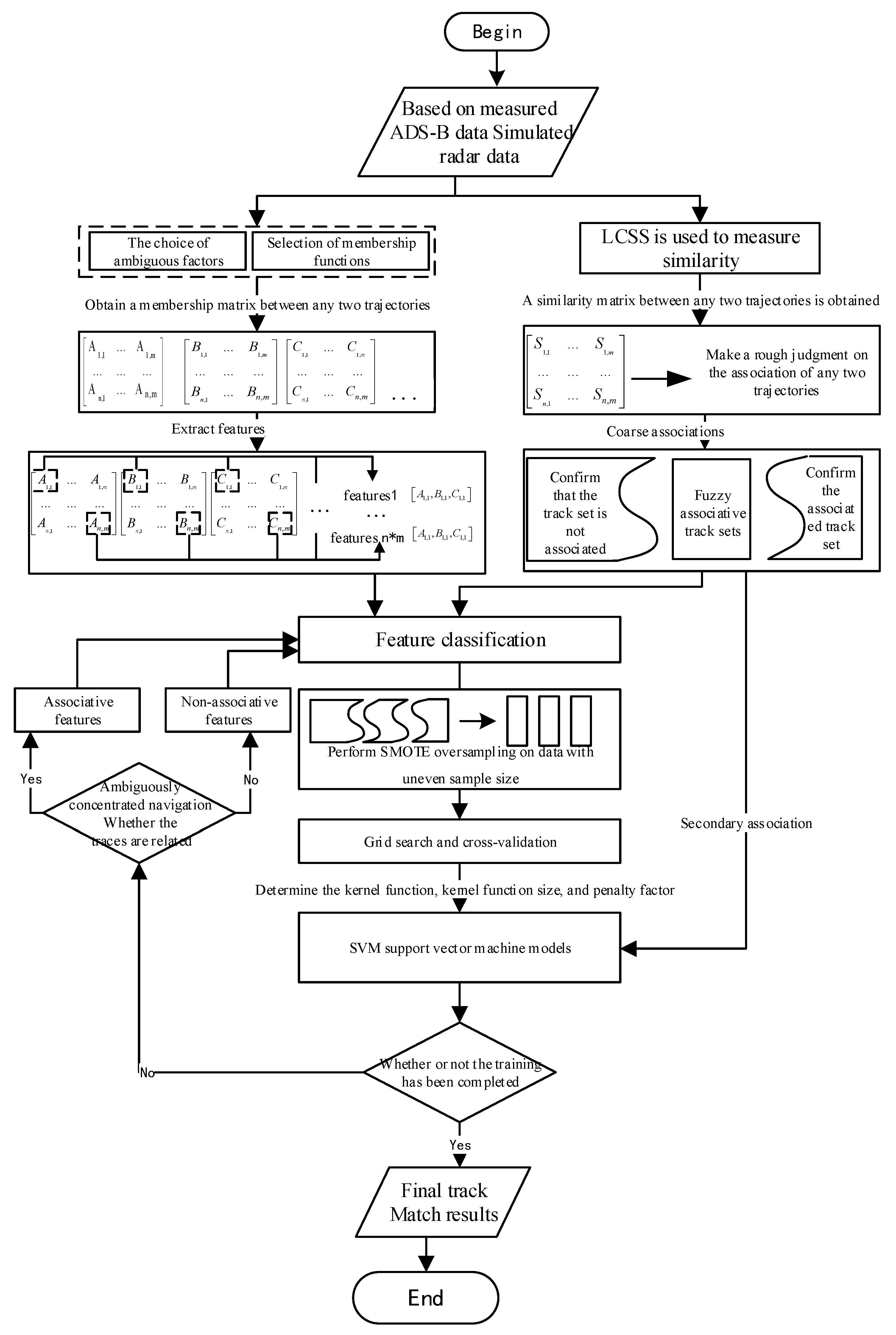
3. Adaptive Track Association Method Based on Automatic Feature Extraction

Figure 1 illustrates the complete workflow of the adaptive track association method, which is based on automatic feature extraction. The process initiates with coordinate transformation of surveillance data, converting radar measurements in polar coordinates and ADS-B data in geodetic coordinates to a unified Cartesian coordinate system. The similarity between radar tracks and ADS-B tracks is subsequently measured via the LCSS algorithm, which generates a similarity matrix. Based on this matrix, tracks are categorized into three distinct groups: the definite association group, the definite unassociated group, and the fuzzy association group. The definite association and unassociated groups are then utilized to extract features via fuzzy mathematics, which are subsequently employed to train a SVM model. Finally, the SVM model is applied to classify and associate the tracks within the fuzzy association group, thereby achieving accurate track associations.

3.1. Surveillance Data Coordinate Transformation

Table 1. ADS-B data.

Year	Month	Day	Hour	Minute	Second	Millisecond	ICAO Address	Flight Number	Latitude (°)	Longitude (°)	Altitude (m)
2022	7	25	9	39	28	539	780294	CSN3792	41.89567566	98.26833542	9852.66
2022	7	25	9	39	31	492	780294	CSN3792	41.89598981	98.27768711	9852.66

and

Table 2. Secondary radar data.

Frame Number	Code Disk	R (Range)	AZ (Azimuth)	EL (Elevation)	Amp (Amplitude)	Beam Num	Filter Num	H (Hour)	M (Minute)	S (Second)
39550	513	17,695.00	46.40	0.14	67	0	6	9	39	27
39553	586	19,795.00	53.06	10.90	72	4	3	9	39	27

show the original format of the ADS-B data and the secondary radar data.

The first step is to measure the similarity between radar tracks and ADS-B tracks via the LCSS algorithm.

The LCSS algorithm is commonly employed to quantify the length of the longest common subsequence between trajectories without requiring continuity. A longer common subsequence indicates a higher degree of similarity between two trajectories [18]. Let $A_i(N)$ denote the N-th point $p_a$ along track $A_i$, and let $R_j(M)$ represent the M-th point $p_b$ along track $R_i$. A predefined distance threshold $\epsilon$ is established, as shown in Equation (1):

$$\left\{\begin{array}{l}LCSS(A_i(N),R_j(M))=0,M=0\hspace{0.17em}\mathrm{or}\hspace{0.17em}N=0\\ LCSS(A_i(N),R_j(M))=LCSS(A_i(N-1),R_j(M-1))+1,||p_a-p_b||<\epsilon \\ LCSS(A_i(N),R_j(M))=\max \left\{\begin{array}{l}LCSS(A_i(N-1),R_j(M))\\ LCSS(A_i(N),R_j(M-1))\end{array}\right.,||p_a-p_b||\ge \epsilon \\ LCSS(T_i,T_j)=\max (LCSS(A_i(N),R_j(M)))\end{array}\right.{\displaystyle \sum _{i=1}^n{(X_i-\overline{X})}^2}$$

(1)

Specifically, the LCSS algorithm measures the similarity between two trajectories within their entire temporal span (from start to end). $p_a$ is a point on the radar track, represented in the spatial rectangular coordinate system; $p_b$ is a point on the ADS-B track, also represented in the spatial rectangular coordinate system.

$$A=\left[\begin{array}{ccc}{A}_{1,1}& \dots & A_{1,m}\\ \dots & \dots & \dots \\ A_{n,1}& \dots & A_{n,m}\end{array}\right]$$

(2)

By employing LCSS to conduct preliminary track matching, we calculate the similarity between all possible track pairs. Here, $n$ denotes the number of ADS-B trajectories, and m represents the number of radar trajectories. Let $A_{i,j}$ denote the similarity measure between ADS-B track $i$ and radar track $j$, with the resulting similarity matrix formulated as an $n\times m$ matrix A.

Through analysis of the similarity matrix, most track groups can be directly classified into associated or nonassociated statuses based on their similarity values. A minority of track groups cannot be directly classified and are defined as ambiguous associations. In this framework, ADS-B and radar trajectories are partitioned into three mutually exclusive categories: confirmed associations, confirmed nonassociations, and ambiguous associations.

• Confirmed associations.

$$\left\{\begin{array}{l}\max \{A_{1j},A_{2j},A_{3j},\dots ,A_{nj}\}=A_{ij}\\ A_{ij}\ge Threshol{d}_U\\ abs(\sec \{A_{1j},A_{2j},A_{3j},\dots ,A_{nj}\}-A_{ij})>Threshol{d}_M\end{array}\right.$$

(3)

In this framework, $Threshol{d}_U$ denotes the threshold for association confirmation, whereas $Threshol{d}_M$ represents the threshold for the difference between the highest and second-highest similarity scores in the similarity matrix between the ADS-B tracks and the $j$th radar track.

When these conditions are satisfied, ADS-B track $i$ and radar track $j$ are identified as an associated track pair. This determination requires the radar track to match precisely one ADS-B track with a high similarity score while exhibiting no other potentially confusable ADS-B tracks with equivalent similarity scores, thus permitting unambiguous association of this track pair.

2.

Confirmed non-associations.

If radar track $j$ is directly correlated with ADS-B track $i$, then $A_{qj}$ is designated a confirmed disassociated track, with $q$ representing any integer in [1, n], excluding $i$.

Alternatively, radar track $j$ can lack a directly associated ADS-B track $i$ and satisfy.

$${\left\{A_{qj}<Threshold\right.}_L,q=[1,2,3,\dots n]$$

(4)

where $Threshol{d}_L$ denotes the confirmed disassociation threshold.

If either of the aforementioned conditions is met, ADS-B track $q$ and radar track $j$ are classified as disassociated track pairs. The minimal correlation similarity between the radar track and ADS-B track, combined with the extremely low probability of originating from the same target, justifies their inclusion in the disassociated track collection.

3.

Ambiguous associations.

If radar track $j$ lacks a directly associated ADS-B track $i$ and satisfies

$$\{A_{qj}>Threshol{d}_L,q=[1,2,3,\dots n]$$

(5)

The ADS-B track $q$ and radar track $j$ are classified as an ambiguously associated track pair. The similarity characteristics of the track pairs in this set are intermediate between those of the associated and non-associated states, representing a primary focus of this study.

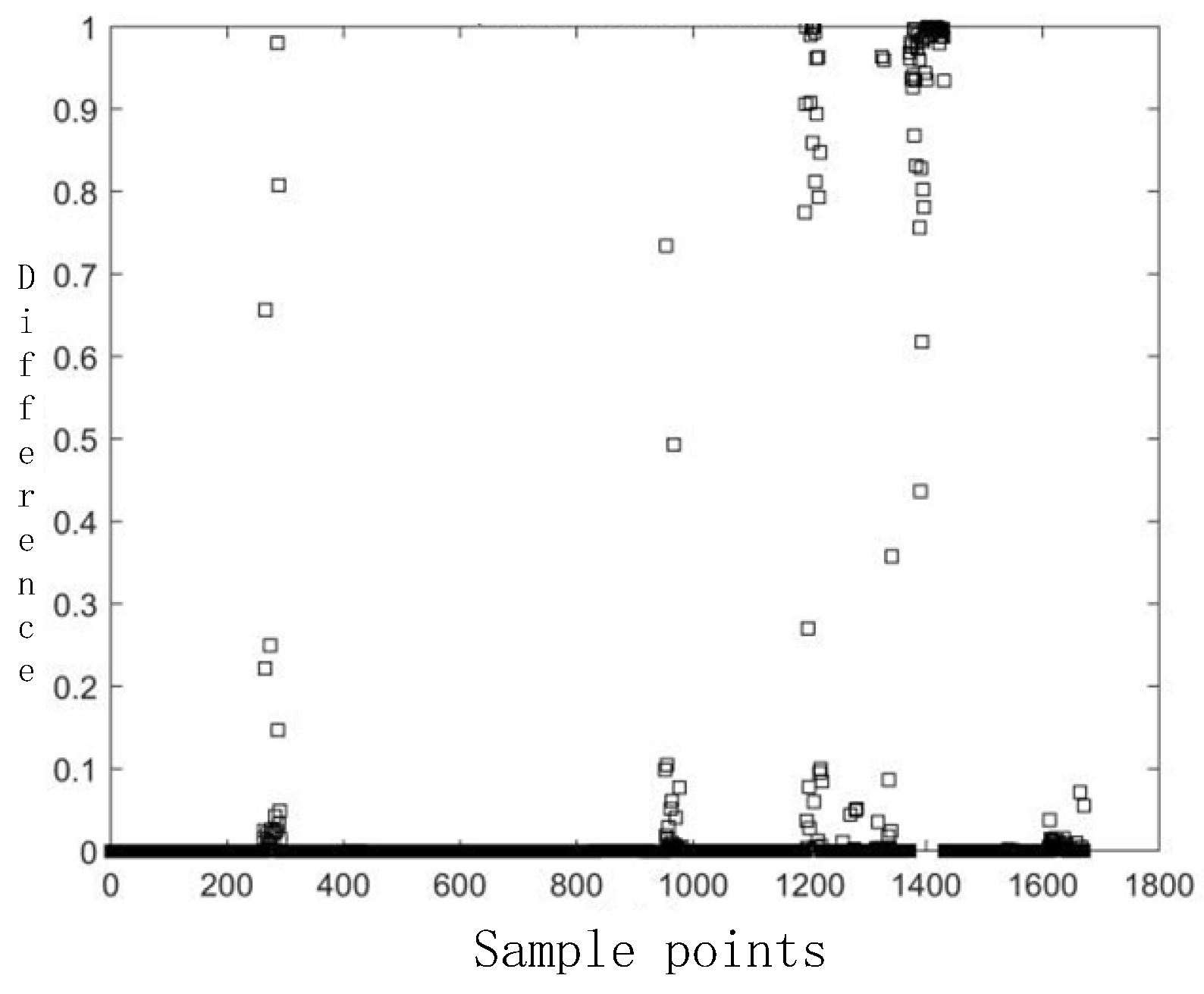
3.2. Sample Oversampling Method

To address the imbalance in the number of confirmed associated and non-associated track pairs, we use the synthetic minority oversampling technique (SMOTE). This method synthesizes training samples for the underrepresented class (confirmed associations) to achieve dataset balance. The process involves selecting a minority class sample and one of its nearest neighbors and then generating a new synthetic sample by interpolating between them.

This study utilizes both confirmed association track pairs and confirmed disassociation track pairs as training data for the SVM classifier. However, the number of confirmed associated track pairs is significantly smaller than that of confirmed non-associated track pairs. Given $n$ radar tracks and $m$ ADS-B tracks, the initial confirmation process can yield at most $w=\max (n,m)$ confirmed association track pairs, with the remaining $n\times m-w$ track pairs categorized as either confirmed non-associated or ambiguously associated track pairs. This imbalance in sample size, exacerbated by increasing $n$ and $m$, can lead to SVM decision boundary distortion and misclassification errors [19]. To address this, the synthetic minority oversampling technique (SMOTE) algorithm is implemented to synthesize new samples, thereby balancing the class distribution. The core idea is to generate synthetic samples through random linear interpolation between each positive class sample (minority samples) and its $k$ nearest neighboring minority class samples. Consider a training dataset $S$, where $S_{\min }\in S$ denotes the minority class samples and $S_{\max }\in S$ represents the majority class samples (with significantly larger volume). For each minority sample $x_i$, its $k$ nearest neighbors $\tilde{X}=\{{\tilde{\mathit{x}}}_1,{\tilde{\mathit{x}}}_2,\cdots ,{\tilde{\mathit{x}}}_k)$ within the same class are identified, where $k$ is determined by the required sample augmentation ratio. A new synthetic sample $x_{\mathrm{new}}=x_i+\delta \times ({\tilde{X}}_j-x_i)$ is generated by linearly interpolating between each minority sample $x_i$ and each ${\tilde{X}}_i(j=1,2,\dots ,k)\in \tilde{X}$, where $\delta$ is a random number uniformly distributed in (0,1).

The SMOTE algorithm generates synthetic samples for the minority class (confirmed associations) to mitigate class imbalance. However, its sensitivity to initial grouping errors is nontrivial: if LCSS thresholds (Equations (3)–(5)) misclassify non-associated tracks as ‘confirmed associations,’ SMOTE will generate synthetic samples that propagate these errors. To mitigate this, we impose stricter similarity thresholds and exclude edge cases (e.g., tracks with ambiguous similarity scores) from oversampling.

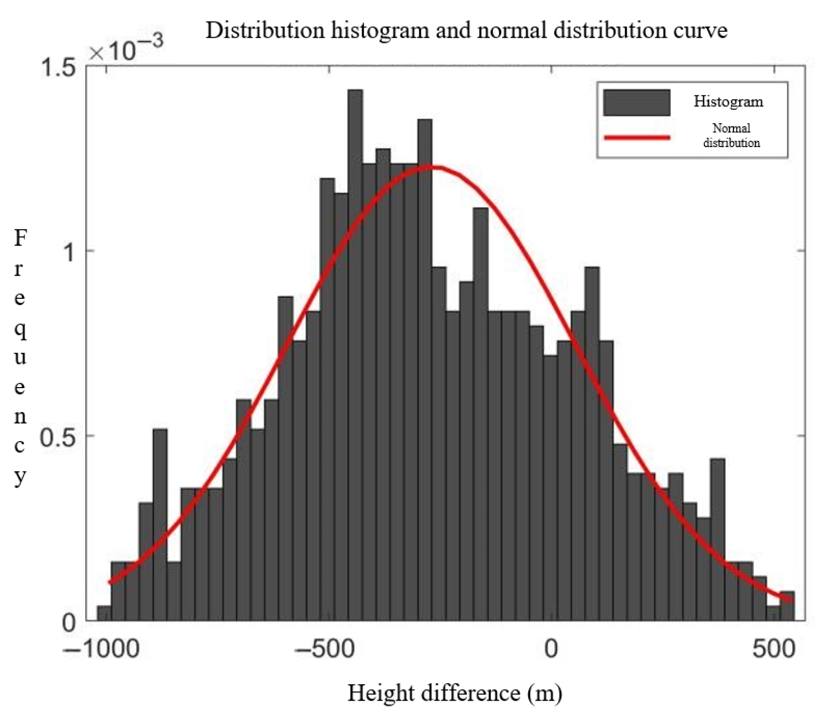
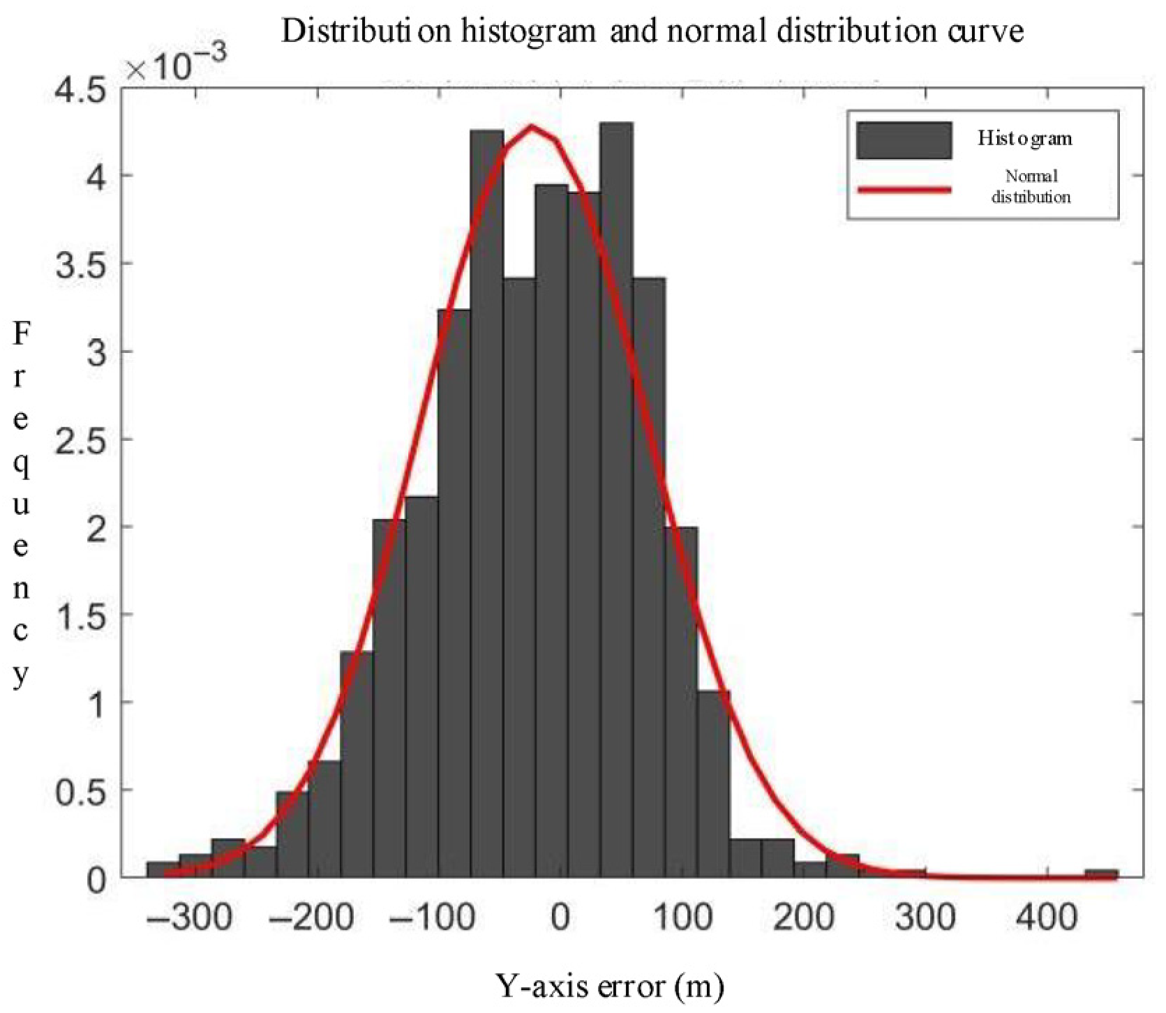
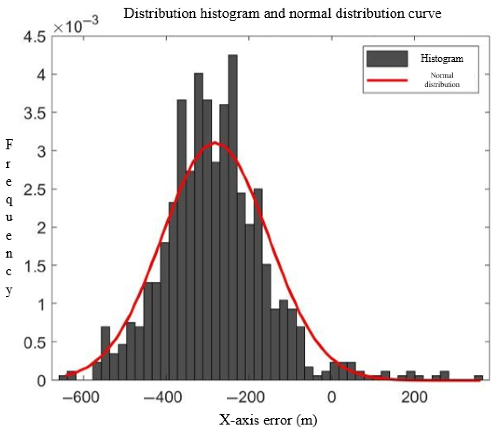
3.3. Membership Function

• Ambiguity Factor Selection.

Fuzzy logic methods are employed in the feature extraction stage to handle the inherent uncertainty and imprecision in the track data. Specifically, fuzzy logic transforms raw error values into fuzzy membership values, which serve as input features for the classification model. This conversion process is termed fuzzification.

This study selects four ambiguity factors: latitude–longitude error, altitude error, speed error, and heading error. Given that positional parameters exert the most significant influence on track associations in aircraft tracking and considering the strict altitude layer constraints imposed during flight operations, positional features are decomposed into latitude–longitude (horizontal position) and altitude (vertical position) components. In addition to positional attributes, aircraft motion characteristics are characterized by speed, whereas track similarity is quantified through heading deviations, both of which serve as critical metrics for track association.

Although maritime track analysis conventionally uses the Haversine formula for geospatial distance calculations between coordinates, this approach is insufficient for aircraft track association. Instead, the Euclidean distance is adopted to compute linear distances between points in a local Cartesian space. To implement this, both radar data (polar coordinates) and ADS-B data (geodetic coordinates) are transformed into a spatial rectangular coordinate system with the radar installation position as the origin, the positive north and west directions as the X-axis and Y-axis, respectively, and the Z-axis constructed according to the right-hand rule:

$$\Delta D_{ijt}=\sqrt{{(x_{iat}-x_{jet})}^2+{(y_{iat}-y_{jet})}^2}$$

(6)

$$\Delta H_{ijt}=|z_{iat}-z_{jet}|$$

(7)

$$\Delta H{E}_{ijt}=|h_{iat}-h_{jet}|$$

(8)

$$\Delta V_{ijt}=|v_{iat}-v_{jet}|$$

(9)

where $(x_{iat},y_{iat},z_{iat})$, $h_{iat}$, and $v_{iat}$ denote the spatial Cartesian coordinates, head, and speed of the $i$ ADS-B track at time $t$, respectively, and $(x_{jet},y_{jet},z_{jet})$, $h_{jet}$, and $v_{jet}$ represent the spatial Cartesian coordinates of the $j$-th radar track at time $t$. The ambiguity factor error set is denoted as $[\Delta D_{ij},\Delta H_{ij},\Delta H{E}_{ij},\Delta V_{ij}]$, representing the horizontal position error, altitude error, and velocity error, respectively.

The fuzzy membership values obtained from the fuzzification process are used as input features for the SVM classifier. Each track pair is represented by a feature vector containing the fuzzy membership values for all four error types.

2.

Membership Function Selection.

An analysis of the error distributions in Figure 2, Figure 3, Figure 4 and Figure 5 reveals that both the track errors and speed errors between the radar tracks and ADS-B tracks exhibit normal distribution characteristics. Consequently, Gaussian functions are adopted as the membership functions for the ambiguity factors:

$$f_k={\displaystyle \frac{{\displaystyle \sum _{q=1}^n\exp [-{\alpha }_k{({\mu }_k(q)/{\sigma }_k)}^2]}}{n}}$$

(10)

where $f_k$ is the mean value of the membership degree for the $k$th ambiguity factor; ${\mu }_k(q)$ is the error value of the $q$th track point for the $k$th ambiguity factor; ${\sigma }_k$ is the variance in the error; and ${\alpha }_k$ is a constant to be determined.

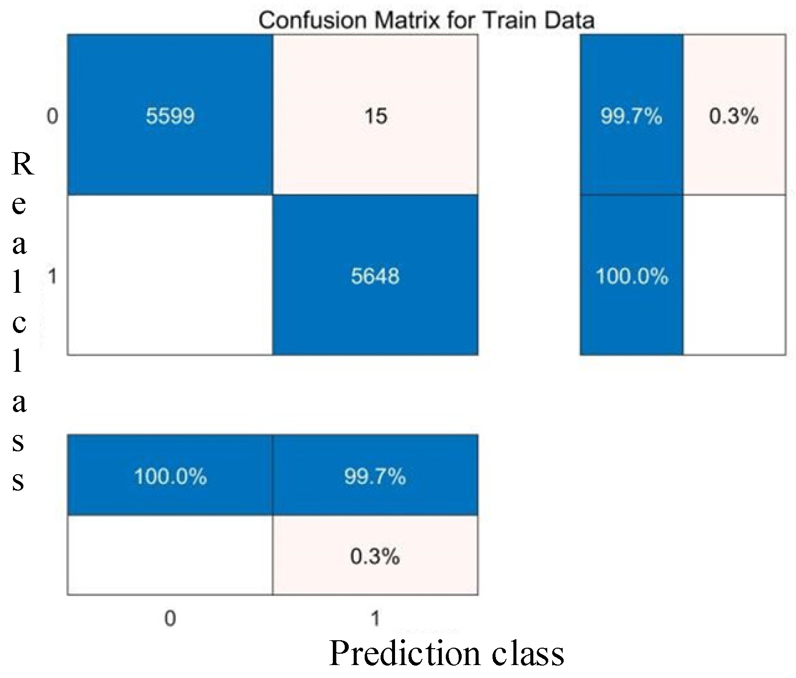
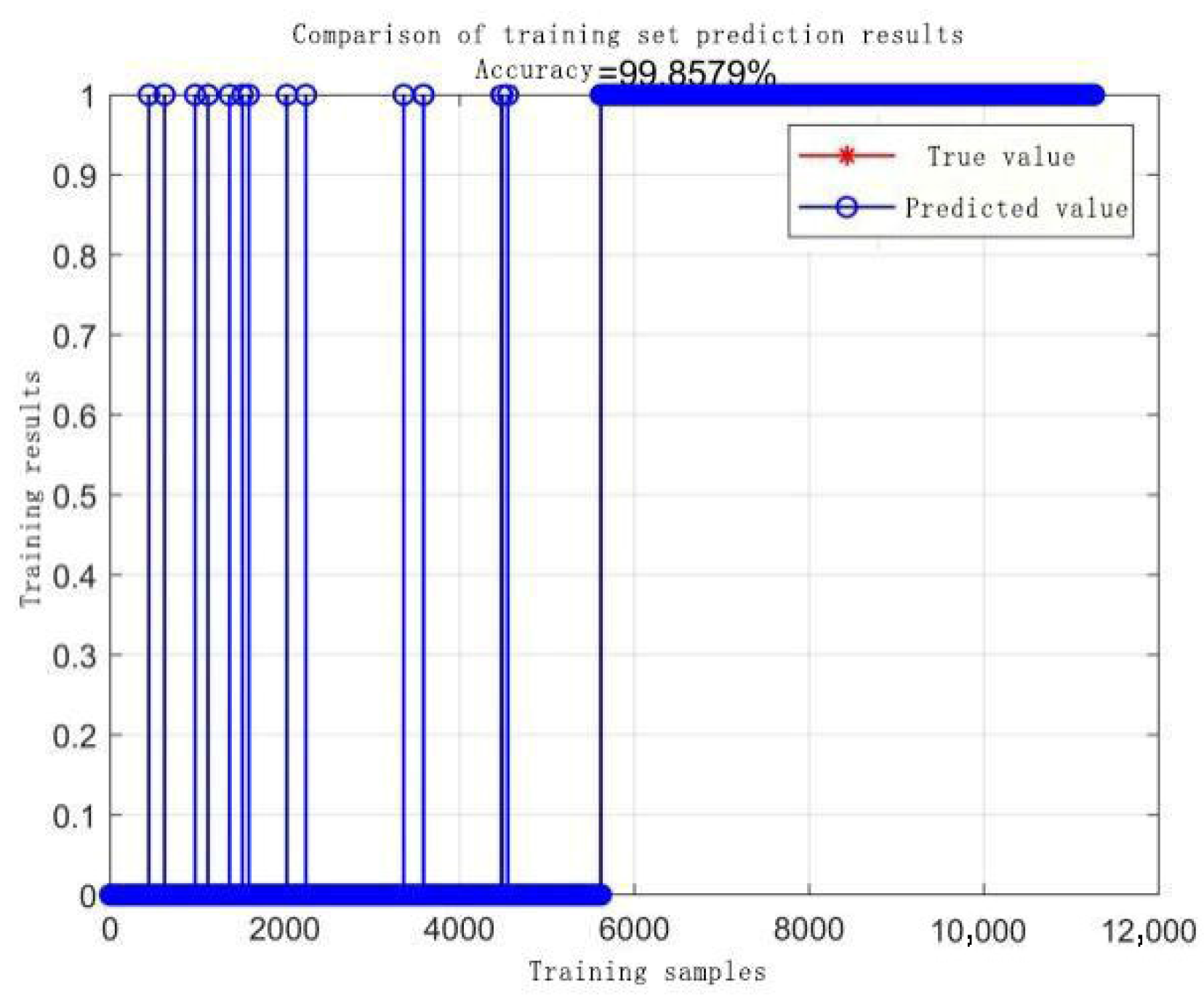
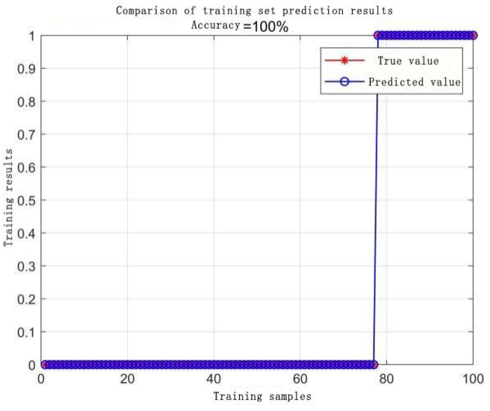
3.4. Classification Model Selection

Finally, we use a SVM to classify the ambiguous associations. The SVM model is trained using the confirmed associated and non-associated track pairs as training samples.

Because of the constrained volume of training data, neither deep learning nor conventional machine learning approaches are viable for training classification models. Since track association inherently constitutes a binary classification task, this study selects SVM as the optimal classifier. SVM, a supervised machine learning paradigm, excels in solving small-sample classification problems by seeking an optimal hyperplane that maximizes the margin between the closest training samples of different classes.

The track association problem addressed herein can be viewed as a variant of binary classification. Previous sections have classified $n\times m$ track pairs (combining $n$ radar tracks and $m$ ADS-B tracks) into three categories through similarity measurement and membership function analysis.

The confirmed associated and confirmed non-associated classes serve as training samples for the SVM, whereas the ambiguous associated class undergoes post-training classification via the trained SVM model (as shown in Figure 6).

For the soft-margin SVM, the objective function and constraints are as follows:

$${\min }_{\omega ,b,\xi }{\displaystyle \frac{1}{2}}\parallel \omega {\parallel }^2+C{{\displaystyle \sum }}_{i=1}^n{\xi }_i$$

(11)

$$s.t. y_i\left({\omega }^T{x}_i+b\right)\ge 1-{\xi }_i,{\xi }_i\ge 0,i=1,\cdots ,n$$

(12)

where $\omega$ is the normal vector of the hyperplane, $C$ is the penalty factor, ${\xi }_i$ is the slack variable, $x_i$ is the feature vector, $y_i$ is the label, $b$ is the threshold, and $n$ is the number of samples.

Considering whether the classification samples are linearly separable, the radial basis function (RBF) kernel, which has strong generalization ability, and the linear kernel, which performs well for high-dimensional features, are tested. Their expressions are as follows:

$$k(x_i,x_j)=x_i^T{x}_j$$

(13)

$$k(x_i,x_j)=exp(-{\displaystyle \frac{\mid |x_i-x_j\mid {\mid }^2}{2{\sigma }^2}})$$

(14)

where Equations (1)–(13) represent a linear kernel and Equations (1)–(14) represent an RBF kernel, where $\sigma$ is the bandwidth of the RBF kernel.

4. Results

4.1. Experimental Environment

To ensure the scientific soundness of our study, we formulated specific hypotheses that our experimental procedures aimed to test. These hypotheses originated from our research objectives and were formulated to verify the efficacy of the proposed adaptive track association approach. To test these hypotheses, we designed a comprehensive experimental plan that includes both simulation and real-world data testing.

Simulation Environment:

Dataset Generation: We generated synthetic datasets with varying levels of noise and data completeness to simulate different operational scenarios.

Baseline Methods: We compared our proposed method with traditional methods (e.g., nearest neighbor, dynamic time warping) and conventional machine learning approaches (e.g., support vector machines, neural networks). Performance Metrics: Precision, recall, F1 score, and computational time were used to evaluate the performance of each method.

Software: MATLAB R2023a, Python 3.9, with libraries such as NumPy, SciPy, and scikit-learn, were used.

Hardware: An Intel Core i7-11700K processor (Intel Corporation, Santa Clara, CA, USA), 32 GB RAM, NVIDIA GeForce RTX 3080 GPU (NVIDIA Corporation, Santa Clara, CA, USA), was used.

Real-World Data Environment:

Dataset Generation: We selected a subset of real-world radar and ADS-B data with known associations for validation.

Evaluation Metrics: The same performance metrics (precision, recall, F1 score, and computational time) were used to assess the effectiveness of our method in the real world.

Data source: Radar and ADS-B data were collected from East China’s A/C-mode secondary radar and ground-based ADS-B receivers.

Data Preprocessing: The raw radar data underwent preprocessing, including track point fusion and noise reduction. The ADS-B data were synchronized with the radar data to ensure temporal alignment.

4.2. Coarse Matching Method Selection

Table 3. Comparison of the efficiencies of the DTW and LCSS algorithms.

	DTW	LCSS
Coarse matching accuracy	70.45%	79.54%
Coarse match time	772.91(s)	51.59(s)

shows that in the study of track coarse matching, the LCSS algorithm demonstrates superior matching efficiency and higher accuracy than the dynamic time warping (DTW) algorithm does. Consequently, LCSS is more suitable as the initial algorithm for track matching in this framework.

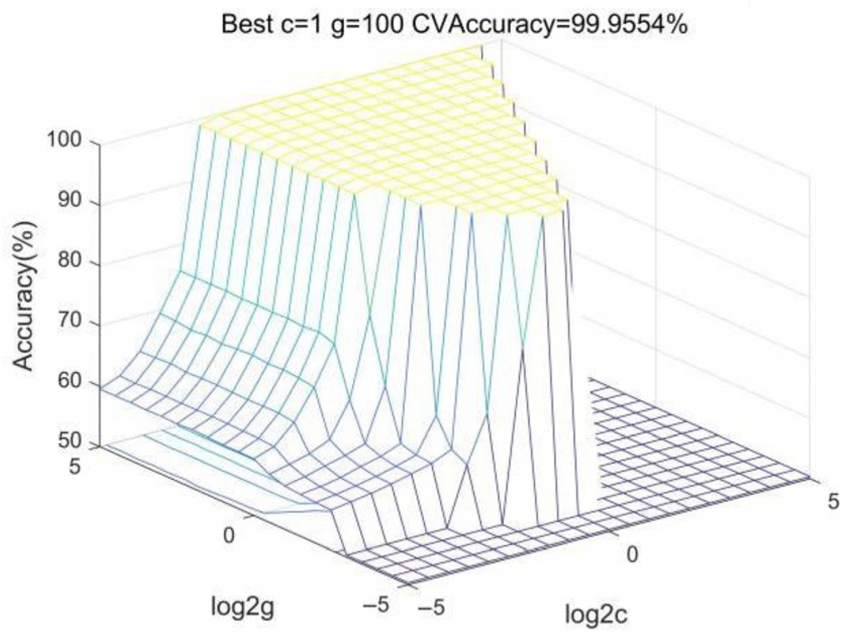
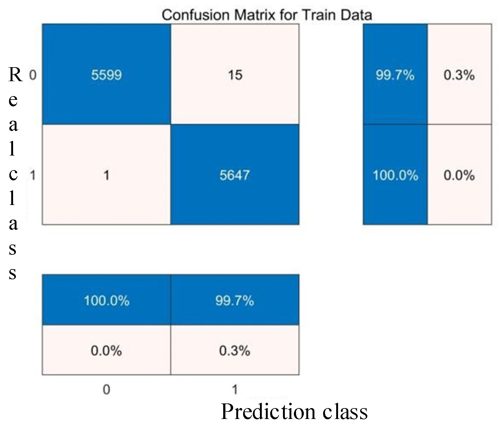
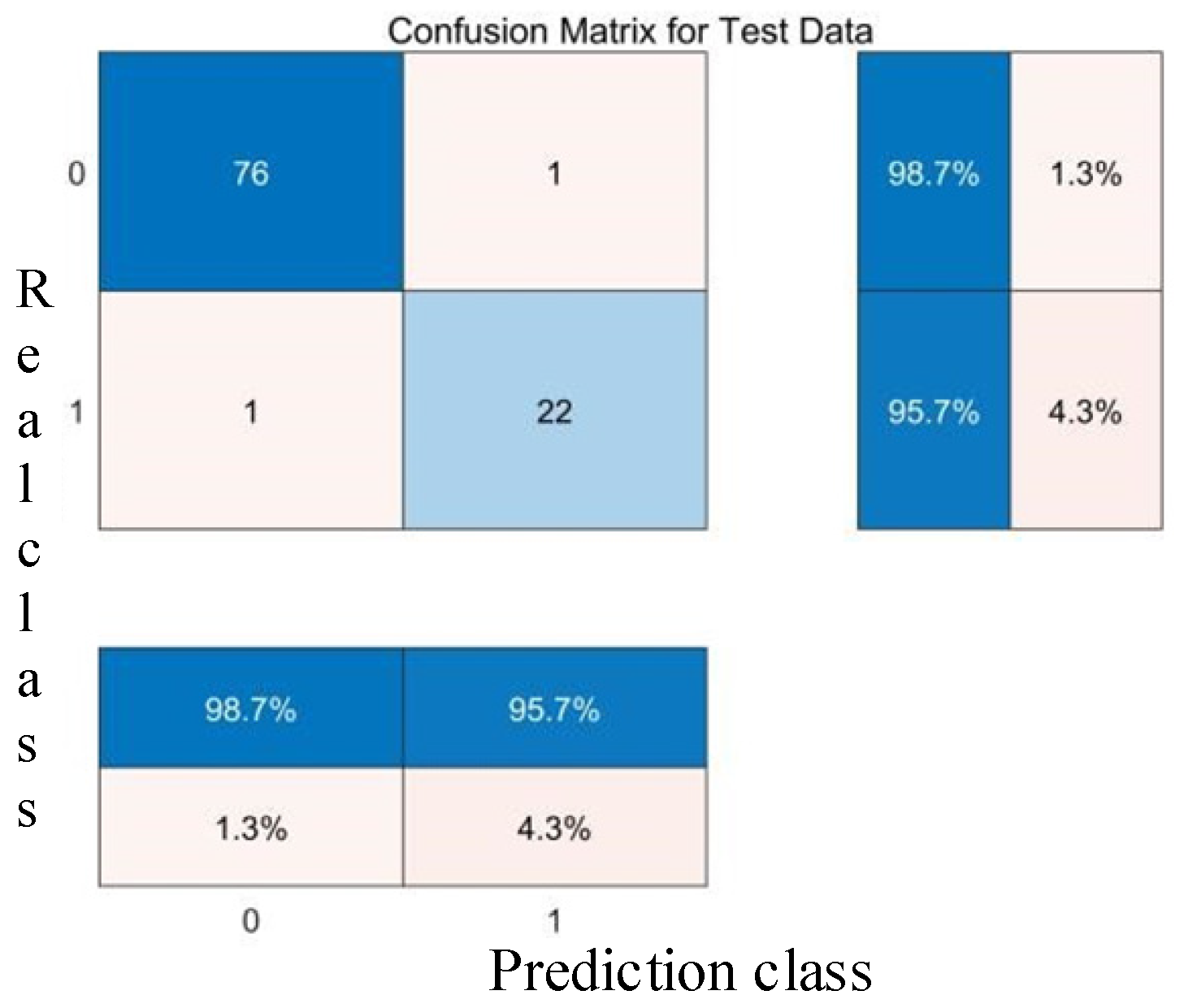
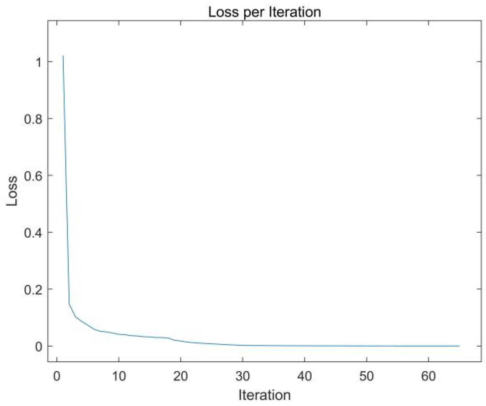
4.3. SVM Kernel Functions and Parameter Determination

This study employed k-fold cross-validation combined with a grid search to determine the optimal kernel functions and their parameters. The dataset used in this study consisted of 11,262 samples, which were divided into training and testing sets at a ratio of 11,162:100.

For the SVM classifier, we tested two kernel functions: the linear kernel and the radial basis function (RBF) kernel. The hyperparameters for each kernel, as determined through grid search and cross-validation, are as follows:

Linear Kernel:

Kernel scale (not applicable for linear kernels):/.

Penalty factor C: 100.

RBF Kernel:

Kernel scale γ: 100.

Penalty factor C: 1.

These hyperparameters were chosen based on their performance in cross-validation, where the generalization error was estimated by averaging the precision and recall across all iterations. The parameter pair that achieved the highest validation accuracy was selected as the optimal pair.

Figure 7 shows that for the RBF kernel with 5-fold cross-validation, the optimal parameters are determined as 1, and the kernel scale is 100, achieving a validation accuracy of 99.9554%.

1.

SVM Classification Results.

(1)

RBF core, Scale 100, Penalty Factor 1:

The comparative analysis of Figure 8, Figure 9, Figure 10, Figure 11, Figure 12, Figure 13, Figure 14 and Figure 15 demonstrates that the linear kernel achieves superior classification performance compared with the RBF kernel in this dataset. Although the RBF kernel function offers greater flexibility for modeling nonlinear relationships, it also increases the difficulty of parameter tuning. The inherent simplicity of the linear kernel not only minimizes overfitting risks but also aligns with the dataset’s high-dimensional characteristics. Specifically, in high-dimensional feature spaces, data points typically exhibit larger interpoint distances, which increase the likelihood of linear separability—a geometric property empirically supported by the linear kernel’s superior experimental results. These empirical observations collectively justify the adoption of the linear kernel for this study.

 

 

(2)

Linear Kernel, Penalty Factor 100:

Figure 12. Linear kernel training set confusion matrix.

Figure 12. Linear kernel training set confusion matrix.

Figure 13. Linear kernel test set confusion matrix.

Figure 13. Linear kernel test set confusion matrix.

Figure 14. Linear kernel training set accuracy rates.

Figure 14. Linear kernel training set accuracy rates.

Figure 15. Linear kernel test set accuracy.

Figure 15. Linear kernel test set accuracy.

4.4. Comparison with Other Methods

• Determination of Comparison Indicators.

Classification results are typically evaluated in terms of precision ($P$), recall ($R$), and the F score:

$$P={\displaystyle \frac{\mathrm{TP}}{\mathrm{TP}+\mathrm{FP}}}$$

(15)

$$R={\displaystyle \frac{\mathrm{TP}}{M}}$$

(16)

where $M$ denotes the total number of track groups, $P$ represents precision, and $R$ indicates recall. Here, $\mathrm{TP}$ (true positive) quantifies the correct association of positive-class track groups, whereas $\mathrm{FP}$ (false positive) refers to the erroneous association of negative-class groups as positive. Precision measures the proportion of correctly associated track groups, whereas recall evaluates the ratio of correctly identified track groups relative to the total population of true positive groups.

The $F$ score is designated the $F_1$ score when the recall and precision accord with equal weighting.

$$F_{\beta }=(1+{\beta }^2)\cdot {\displaystyle \frac{P\cdot R}{({\beta }^2\cdot P)+R}}$$

(17)

When $\beta$ = 1 in the F score formulation, it is termed the $F_1$ score.

$$F_{\beta }=2\cdot {\displaystyle \frac{P\cdot R}{P+R}}$$

(18)

2.

Determination of the comparison methods.

The benchmark analysis encompassed three established track association approaches:

Back propagation-based feedforward neural network method [13]: A single-hidden-layer BP network is employed, with radar and automatic identification system (AIS) target features, including distance, bearing, speed, and course, as input nodes (totaling eight dimensions). The network outputs binary results, namely, $Y$ for associated trajectories and $N$ for non-associated trajectories, followed by training using labeled data.

Deep Learning-enhanced Method [14]: To enhance the generalization performance, scene features and track features are separately fed into a dual-input deep learning framework. Scene features are extracted via CNN (convolutional neural network) modules to improve model robustness against environmental variations.

Fuzzy Membership Degree Method: This method employs a three-stage computational framework. This approach calculates fuzzy factor membership degrees and determines their respective weights through fuzzy logic rules. A weighted summation of membership degrees is calculated, followed by application of an association threshold to determine final track classification.

Owing to the distinct validation environments of the compared methods, Method 2 employed pure simulation data and GPU-accelerated PyTorch (v1.8.0)-based deep learning models, whereas Methods 1 and 3 utilized real-world sensor data with added noise. All experiments were conducted using Python 3.9, with CUDA 11.1 for GPU acceleration where applicable. This study, therefore, designed two categories of simulation scenarios for comprehensive model evaluation

Scenario 1 replicated the simulation framework proposed in the literature [14].

Table 4. Comparison of association accuracy rates.

Associative Method	Deep Learning	Methods of This Article
Correct correlation rate	87.47%	94.95%
Error correlation rate	8.76%	5.05%

shows that the deep learning method outperforms the Associative Method in terms of correct correlation rate, achieving a higher rate of 94.95% compared to the rate of 87.47% achieved by the Associative Method. Additionally, the error correlation rate for deep learning is significantly lower at 5.05%, compared to 8.76% for the Associative Method, indicating that deep learning provides more accurate and reliable results in this context.

Based on a comparative analysis with deep learning approaches, the latter achieves enhanced generalization capability by learning multiscenario features and their corresponding scene-specific patterns. Compared with conventional techniques, this method significantly improves the association accuracy. However, our proposed methodology circumvents scene dependency by dynamically extracting novel scene-specific features in each new environment. Consequently, it exhibits superior generalizability and association accuracy across diverse scenarios compared with the approach presented in the literature [14].

Scenario 2 was generated by introducing noise into the ADS-B data. Based on different noise magnitudes, scene 2 was divided into a class a large error scene and a class b small error scene. Prior to testing in Scenario 2, a BP network model specifically tailored to our dataset underwent pretraining.

The following is the BP network model trained on the data in this paper.

As shown in Figure 16, Figure 17 and Figure 18, the BP model achieves the predefined loss threshold after 67 iterations of training. Although there were some sample points with large deviations, the point difference of most samples was small. Notably, the model exhibits robust generalization capability, attaining 96.29% association accuracy on the test dataset. This pretrained model subsequently serves as the baseline for comparative evaluations across all methods.

Both the BP neural network and traditional fuzzy membership degree function-based association methods share a common limitation. As illustrated in Figure 19 and Figure 20, there exists an inherent trade-off between recall and precision. Specifically, decreasing the association threshold continuously improves recall at the expense of reduced precision, whereas increasing the threshold inversely diminishes recall while enhancing precision.

Scenario 2(a): Synthetic datasets.

Systematic errors:

X/Y/Z axes: ±2000 m displacement.

Heading: ±1° deviation.

Random errors:

X/Y axes: Additive Gaussian noise with an average height of 300 m.

Z axis: Additive Gaussian noise with an average height of 400 m.

Heading: Additive Gaussian noise with an average of 1°.

Rotation perturbations:

Random rotation errors between 1° and 2°.

Track integrity handling:

Fifteen trajectories were randomly selected, and 40% of their points were removed.

From the remaining trajectories, another 15 trajectories were randomly selected, and 60% of their points were deleted.

Track quantity control:

Ten complete simulation trajectories were randomly eliminated.

Table 5. Association results of this method.

Threshold	TP	FP	P%	R%	F1%
0.8	64	1	98.46	84.21	90.78
0.7	63	2	96.92	82.89	89.36
0.6	63	2	96.92	82.89	89.36
0.5	63	2	96.92	82.89	89.36
0.4	63	2	95.46	82.89	88.73
0.3	63	2	95.46	82.89	88.73

,

Table 6. Association results based on the membership function.

Threshold	TP	FP	P%	R%	F1%
0.8	/	/	/	/	/
0.7	8	0	100	10.53	19.05
0.6	21	0	100	27.63	43.30
0.5	38	2	95	50	65.52
0.4	52	5	91.23	68.42	78.12
0.3	60	13	82.19	78.94	80.53

and

Table 7. Association results based on the BP network.

Threshold	TP	FP	P%	R%	F1%
0.8	22	0	100	28.95	44.90
0.7	25	1	96.15	32.89	49.01
0.6	30	3	90.91	39.47	55.04
0.5	36	3	92.31	47.37	62.61
0.4	44	3	93.61	57.89	71.54
0.3	53	5	91.38	69.74	79.10

show that the track association method proposed in this paper achieves excellent comprehensive performance under different thresholds, maintains the balance of high precision and recall, and has a stable F1 score, indicating good stability. In contrast, the membership function-based method sacrifices precision when the recall is improved, whereas the BP network-based method has high precision but low recall at high thresholds. As the threshold decreases, the recall increases, but the precision decreases.

Scenario 2(b): Synthetic datasets.

Systematic errors:

X/Y/Z axes: ±1000 m displacement.

Heading: ±1° deviation.

Random errors:

X/Y axes: Additive Gaussian noise with an average height of 300 m.

Z-axis: Additive Gaussian noise with an average height of 400 m.

Heading: Additive Gaussian noise with an average of 1°.

Rotation perturbations:

Random rotation errors between 1° and 2°.

Track integrity handling: Fifteen trajectories were randomly selected, and 40% of their points were removed from the remaining trajectories; another 15 trajectories were randomly selected, and 60% of their point tracks were deleted.

Quantity control: Ten complete simulation trajectories were randomly eliminated.

Table 8. Correlation results of this method.

Threshold	TP	FP	P%	R%	F1%
0.8	72	1	98.63	94.74	96.65
0.7	72	1	98.63	94.74	96.65
0.6	73	1	98.65	96.05	97.33
0.5	73	1	98.65	96.05	97.33
0.4	73	1	98.65	96.05	97.33
0.3	73	1	98.65	96.05	97.33

,

Table 9. Association results based on the membership function.

Threshold	TP	FP	P%	R%	F1%
0.8	9	0	100	11.84	21.17
0.7	23	0	100	30.26	46.46
0.6	50	0	100	65.79	79.37
0.5	63	0	100	82.90	90.65
0.4	72	1	98.63	94.74	96.65
0.3	74	1	98.68	98.68	98.68

and

Table 10. Association results based on the BP network.

Threshold	TP	FP	P%	R%	F1%
0.8	66	2	97.06	86.84	91.67
0.7	66	3	95.65	86.84	91.03
0.6	67	3	95.71	88.16	91.78
0.5	67	4	94.37	88.16	91.16
0.4	67	4	94.37	88.16	91.16
0.3	69	4	94.52	90.79	92.62

show that the proposed track association method has excellent accuracy and recall at each threshold, and the F1 score is also high, indicating good performance and stability. In contrast, the accuracy of the membership function-based method decreases when the recall rate is improved, whereas that of the BP network-based method is stable, but the overall performance is slightly inferior.

According to the simulation results, the traditional fuzzy membership degree method achieves the highest precision under high association thresholds, whereas our proposed method demonstrates superior precision over both the traditional method and the BP-based approach at low thresholds. Notably, in Scenario 2(a), the traditional method results in significant precision degradation when the threshold decreases. Our method consistently outperforms the other two approaches in both scenarios. In Scenario 2(a) (large noise), SMOTE-augmented training reduced the number of errors by ≤5% compared with nonaugmented SVM, demonstrating robustness to moderate initial errors. However, extreme noise (>2000 m) increased error propagation by 12%, underscoring the need for strict LCSS prefiltering. Although the BP-based method maintains relatively stable recall in Scenario 2(b), its recall decreases sharply under high thresholds in Scenario 2(a). Similarly, the traditional fuzzy method experiences a substantial decrease in recall in both scenarios when the threshold is elevated. By establishing fuzzy association groups, our method decouples the threshold setting from precision–recall trade-offs. Consequently, both precision and recall are maintained at elevated levels independent of threshold adjustments.

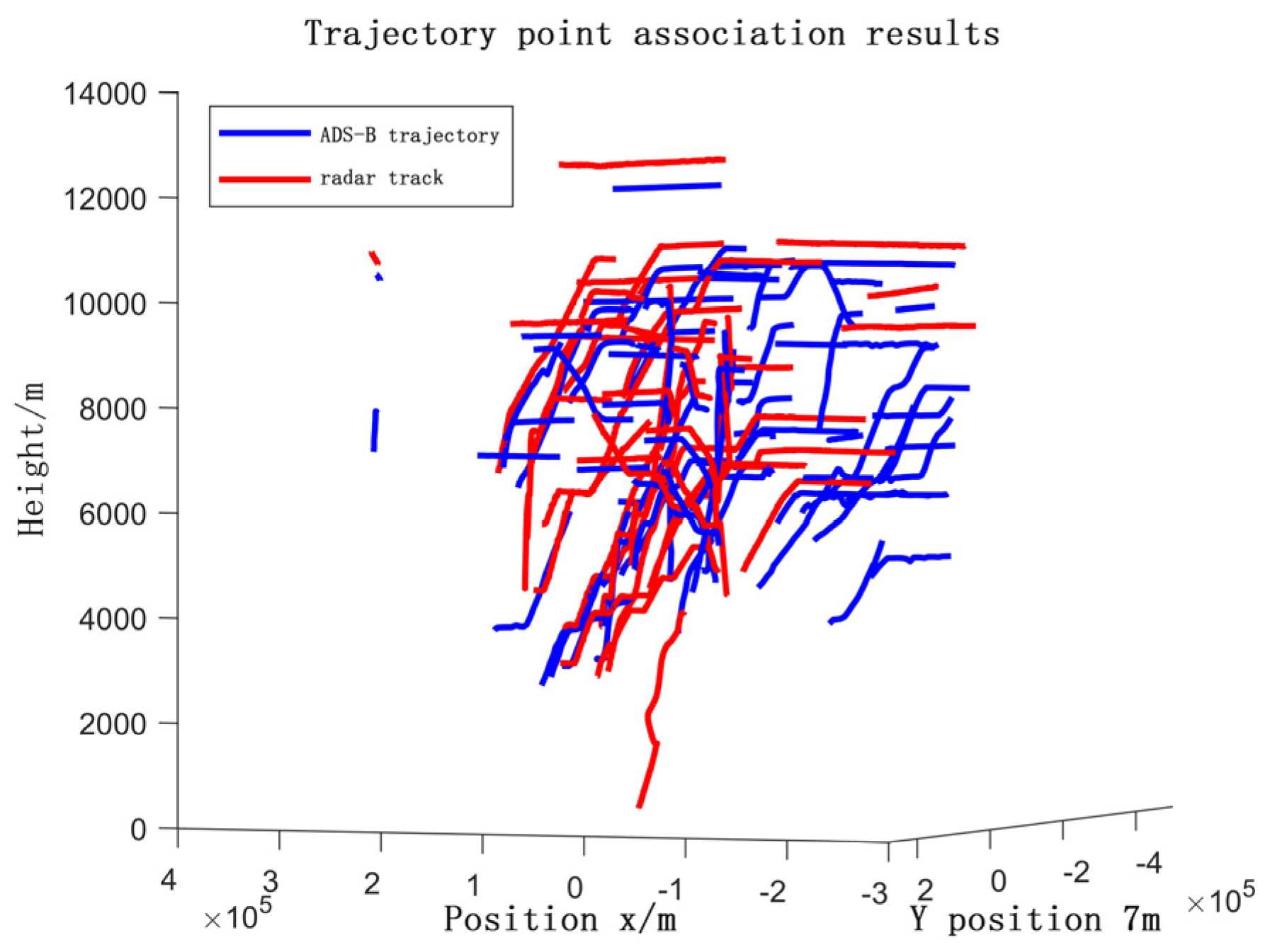
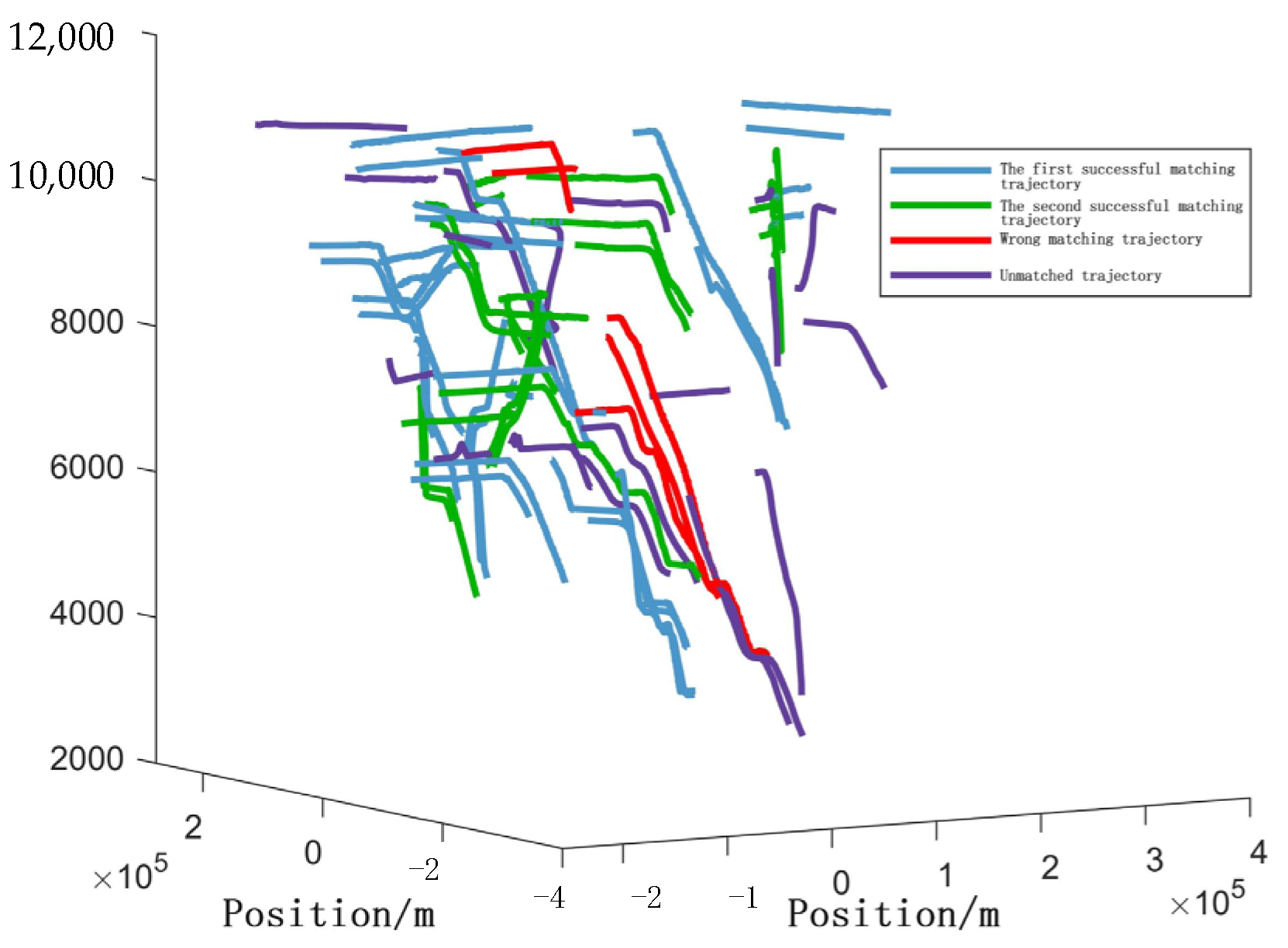
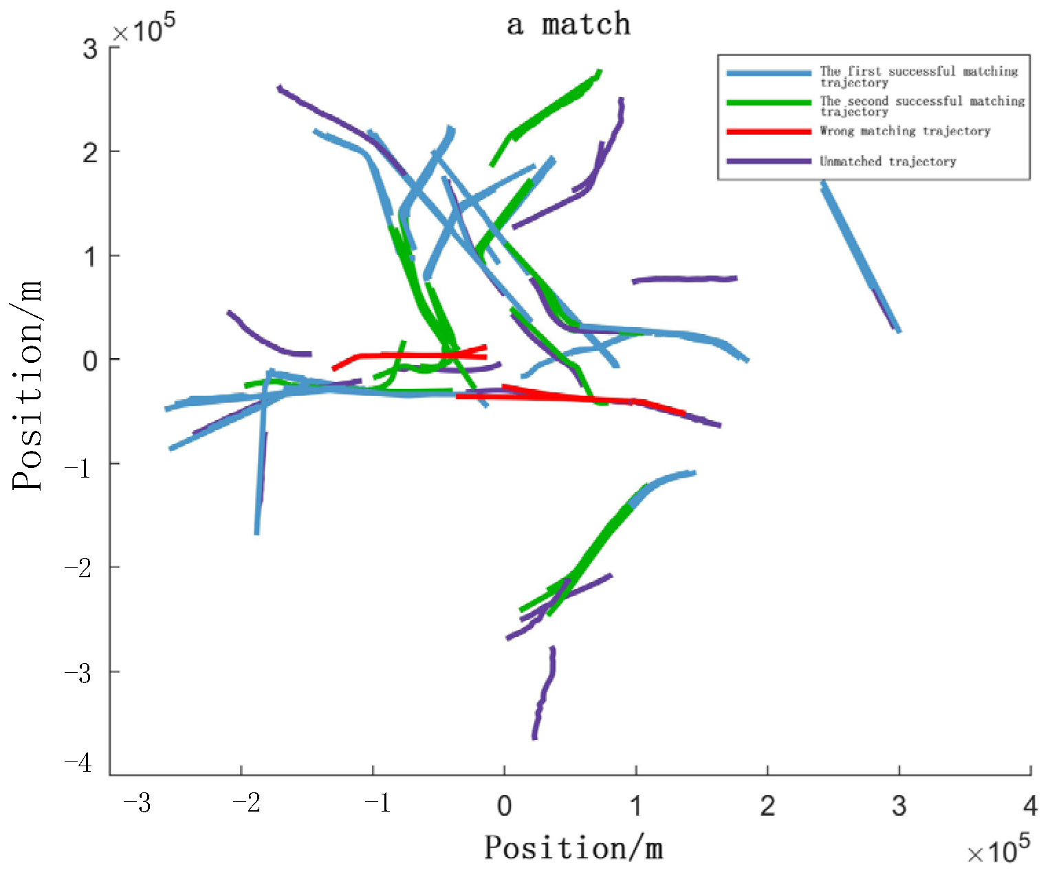
4.5. Field Validation (Real Datasets)

A dataset was acquired from A/C-mode secondary radar installations and terrestrial ADS-B receivers in East China.

(1)

Radar Data Preprocessing.

The raw radar data (non- CAT048 [20]) underwent preprocessing, including track point fusion. The fusion results are visualized in the following Figure 21 and Figure 22.

Individual radar track points associated with track point associations were used to form continuous target trajectories.

(2)

Track Correlation.

Three correlation methods were applied for track matching. Figure 23 compares the performance of our method against that of the baseline approaches.

The measured results shown in Figure 23, Figure 24 and Figure 25 and

Table 11. Comparison of the efficiency of the three algorithms.

Method	Time (s)
Based on the BP network	120.81 s
Based on the traditional fuzzy membership function	25.17 s
Methods of this article	34.66 s

,

Table 12. Based on the BP network.

(BP) Threshold	Precision (%)	Recall (%)
0.90	99.82%	56.57%
0.85	94.43%	56.73%
0.80	89.18%	56.73%
0.75	85.46%	58.89%
0.70	81.76%	61.21%

,

Table 13. Methods of this article.

(Methods of This Article) Threshold	Precision (%)	Recall (%)
0.90	99.97	59.05
0.85	95.36	62.60
0.80	90.72	65.69
0.75	87.94	64.45
0.70	84.85	63.69

and

Table 14. Based on the traditional fuzzy membership function.

(Traditional) Threshold	Precision (%)	Recall (%)
0.90	99.89	33.86
0.85	96.60	47.77
0.80	93.20	61.21
0.75	81.92	61.36
0.70	70.64	61.21

indicate that the experimental outcomes align with the previous simulation results. When a high threshold is set, the traditional fuzzy membership method achieves higher precision but significantly sacrifices the recall rate. The BP neural network-based method demonstrates satisfactory performance in both the precision and recall metrics; however, its computational time consumption is 4.8 times greater than that of the traditional fuzzy membership approach. In contrast, this study’s proposed method demonstrates superior performance across both the precision and recall metrics while requiring merely one-third of the computational time of the BP neural network approach.

5. Conclusions

This study proposes an adaptive track association method based on automatic feature extraction, which integrates the LCSS algorithm, fuzzy mathematics, and SVM to address the challenges of track association between radar and ADS-B data. Compared with conventional methods, the proposed method significantly improves both computational efficiency and accuracy while effectively resolving the inherent precision–recall trade-off of traditional fuzzy membership function-based approaches.

Compared with conventional machine learning approaches and deep learning methods with strong generalization capabilities, this method demonstrates superior computational efficiency and enhanced scenario adaptability across diverse environments. Importantly, it resolves the inherent precision–recall trade-off characteristic of traditional fuzzy membership function-based methods. Moreover, the proposed adaptive feature extraction methodology can be extended to other machine learning-based sample labeling stages, thereby establishing a systematic methodology for tracking association tasks.

However, this study also has the following limitations: While SMOTE improved SVM performance, its dependency on accurate LCSS groupings remains a limitation. Future work will integrate error-aware oversampling techniques, such as SMOTE-ENN (Edited Nearest Neighbors), to automatically prune misclassified synthetic samples. A key limitation of this work stems from the Gaussianity assumption underlying the membership functions. To address non-Gaussian distribution characteristics in real-world applications, future research will explore two main approaches: (1) kernel density estimation (KDE)-based membership functions, which are distribution-agnostic and adaptive, and (2) fuzzy clustering algorithms (e.g., Gustafson–Kessel) for automatically learning optimal membership shapes directly from data. Although these methods are anticipated to improve model performance in complex environments, they inherently incur greater computational demands, which is a necessary trade-off for enhanced robustness.

References

1. He, Y.; Song, Q.; Xiong, W. A track registration-correlation algorithm based on Fourier transform. Acta Aeronaut. Astronaut. Sin. 2010, 31, 356–362. (In Chinese) [Google Scholar]
2. Blasch, E. Handbook of Multisensor Data Fusion: Theory and Practice; CRC Press: Boca Raton, FL, USA, 2009. [Google Scholar]
3. Kanyuck, A.J.; Singer, R.A. Correlation of multiple-site track data. IEEE Trans. Aerosp. Electron. Syst. 1970, 2, 180–187. [Google Scholar] [CrossRef]
4. Kaplan, L.M.; Bar-Shalom, Y.; Blair, W.D. Assignment costs for multiple sensor track-to-track association. IEEE Trans. Aerosp. Electron. Syst. 2008, 44, 655–677. [Google Scholar] [CrossRef]
5. Aziz, A.M. A new nearest-neighbor association approach based on fuzzy clustering. Aerosp. Sci. Technol. 2013, 26, 87–97. [Google Scholar] [CrossRef]
6. Blackman, S.S.; Popoli, R. Design and Analysis of Modern Tracking Systems; Artech House: Norwood, MA, USA, 1999; pp. 608–628. [Google Scholar]
7. Magdy, N.; Sakr, M.A.; Mostafa, T.; El-Bahnasy, K. Review on trajectory similarity measures. In Proceedings of the 2015 IEEE Seventh International Conference on Intelligent Computing and Information Systems (ICICIS), Cairo, Egypt, 12–14 December 2015; IEEE: Piscataway, NJ, USA, 2015. [Google Scholar] [CrossRef]
8. Xu, Q.; Zhao, K.; Qu, D.; Liu, G. LSCC-based fast matching method of target trajectory rule. Syst. Eng. Electron. 2022, 44, 1263–1269. (In Chinese) [Google Scholar]
9. Tian, W. Reference pattern-based track-to-track association with biased data. IEEE Trans. Aerosp. Electron. Syst. 2016, 52, 501–512. [Google Scholar] [CrossRef]
10. Tian, W.; Wang, Y.; Shan, X.; Yang, J. Track-to-Track Association for Biased Data Based on the Reference Topology Feature. IEEE Signal Process. Lett. 2014, 21, 449–453. [Google Scholar] [CrossRef]
11. Sönmez, H.H.; Hocaoğlu, A.K. Asynchronous track-to-track association algorithm based on reference topology feature. Signal Image Video Process. 2022, 16, 789–796. [Google Scholar] [CrossRef]
12. Zhang, Y.; Wu, K.; Guo, J.; Ge, Z.; Zhang, B. Adaptive sequential track-association algorithm based on data quality assessment. Syst. Eng. Electron. 2022, 44, 3477–3485. (In Chinese) [Google Scholar]
13. Chen, Z.T.; Chen, J.P.; Pan, L. Identification method for vessel interrupt track correlating based on fuzzy membership degree. J. Appl. Sci. 2023, 41, 296–310. (In Chinese) [Google Scholar]
14. He, Y.; Peng, Y.J.; Lu, D. Fuzzy track correlation algorithms for multitarget and multisensor tracking. Acta Electron. Sin. 1998, 15–19+9. (In Chinese) [Google Scholar]
15. Zhang, X.; Zheng, J.; Lin, C.; Hu, X. Target Association Algorithm and Simulation for Radar and AIS Based on BP Network. J. Syst. Simul. 2015, 27, 506–514. (In Chinese) [Google Scholar]
16. Cui, Y.Q.; He, Y.; Tang, T.T.; Xiong, W. A deep learning track correlation method. Acta Electron. Sin. 2022, 50, 759–763. (In Chinese) [Google Scholar]
17. Cao, Y.; Cao, J.; Zhou, Z. Track Segment Association Method Based on Bidirectional Track Prediction and Fuzzy Analysis. Aerospace 2022, 9, 274. [Google Scholar] [CrossRef]
18. Wei, L.-X.; He, X.-H.; Teng, Q.-Z.; Gao, M.-L. Trajectory classification based on hausdorff distance and longest common subsequence. J. Electron. Inf. Technol. 2013, 35, 784–790. (In Chinese) [Google Scholar] [CrossRef]
19. Majzoub, H.A.; Elgedawy, I. AB-SMOTE: An Affinitive Borderline SMOTE Approach for Imbalanced Data Binary Classification. Arab. J. Sci. Eng. 2020, 45, 3205–3222. [Google Scholar] [CrossRef]
20. CAT048; Surveillance Data Exchange—Part 48: Category 048—Monoradar Target Reports. Eurocontrol: Brussels, Belgium, 2024.
Figure 1. Adaptive track association method based on automatic feature extraction.
Mathematics 13 02403 g001
Figure 2. y = 0.001212 e ( x + 229.7630 ) 2 217800 , undetermined coefficient = 820, height error distribution histogram, and distribution curve.
Mathematics 13 02403 g002
Figure 3. y = 0.004236 e ( x + 12.15 ) 2 1152 , undetermined coefficient = 265, Y-axis error distribution histogram, and distribution curve.
Mathematics 13 02403 g003
Figure 4. y = 0.0027 e ( x + 219.579 ) 2 42100 , undetermined coefficient = 350, X-axis error distribution histogram, and distribution curve.
Mathematics 13 02403 g004
Figure 5. y = 0.031656 e ( x + 2.5280 ) 2 2 × 12.61 2 , undetermined coefficient = 33, velocity error distribution histogram, and distribution curve.
Mathematics 13 02403 g005
Figure 6. SVM classification diagram.
Mathematics 13 02403 g006
Figure 7. SVC parameter selection result.
Mathematics 13 02403 g007
Figure 8. Confusion matrix of the RBF core training set.
Mathematics 13 02403 g008
Figure 9. Confusion matrix of the RBF core test set.
Mathematics 13 02403 g009
Figure 10. Accuracy rates of the RBF core training set.
Mathematics 13 02403 g010
Figure 11. Accuracy of the RBF core test set.
Mathematics 13 02403 g011
Figure 16. Loss rates of the BP neural network.
Mathematics 13 02403 g016
Figure 17. BP neural network test results.
Mathematics 13 02403 g017
Figure 18. Differences in the prediction results of the BP neural network.
Mathematics 13 02403 g018
Figure 19. Relationships between the double threshold and the recall rate based on the BP network.
Mathematics 13 02403 g019
Figure 20. Relationships between the double threshold and accuracy of the BP network.
Mathematics 13 02403 g020
Figure 21. Radar data preprocessing and tracking point fusion results.
Mathematics 13 02403 g021
Figure 22. Radar track point association results.
Mathematics 13 02403 g022
Figure 23. Comparison of the recall rates and accuracy rates of the three methods.
Mathematics 13 02403 g023
Figure 24. Association results of this method.
Mathematics 13 02403 g024
Figure 25. Association result (top view).
Mathematics 13 02403 g025