Maximum-Likelihood Estimation for the Zero-Inflated Polynomial-Adjusted Poisson Distribution

Abstract

We propose the zero-inflated Polynomially Adjusted Poisson (zPAP) model. It extends the usual zero-inflated Poisson by multiplying the Poisson kernel with a nonnegative polynomial, enabling the model to handle extra zeros, overdispersion, skewness, and even multimodal counts. We derive the maximum-likelihood framework—including the log-likelihood and score equations under both general and regression settings—and fit zPAP to the zero-inflated, highly dispersed Fish Catch data as well as a synthetic bimodal mixture. In both cases, zPAP not only outperforms the standard zero-inflated Poisson model but also yields reliable inference via parametric bootstrap confidence intervals. Overall, zPAP is a clear and tractable tool for real-world count data with complex features.

1. Introduction

Count data with an excessive number of zeros are widespread in fields such as ecology, health economics, transportation, criminology, and insurance analytics. In practice, observed zeros often arise from two distinct mechanisms: some zeros result from stochastic variability in a Poisson-like process (for example, a rare event that simply does not occur), while other zeros reflect a structural process that deterministically yields zero counts. Standard Poisson regression, which assumes equidispersion and independent event occurrences, cannot distinguish between these mechanisms. As a result, it frequently produces biased parameter estimates, underestimates standard errors, and delivers suboptimal predictive performance when applied to zero-inflated data.

Zero-Inflated Poisson (ZIP) models address part of this complexity by introducing a two-part mixture: one component that governs structural zeros and another that governs the count distribution. However, even this mixture imposes strict constraints on the shape of the count component. In many real-world applications, count distributions exhibit skewness, multimodality, heavy tails, or degrees of zero-inflation that exceed what a single Poisson family can accommodate. Empirical distributions may show multiple peaks due to mixed subpopulations, or have tails that are heavier than what the standard Poisson model allows. This can lead to systematic discrepancies in higher-order moments and tail probabilities.

Semiparametric and nonparametric extensions, such as transformation models, infinite-mixture formulations, and kernel-based likelihoods, have been proposed to capture these complex distributional characteristics. These methods improve flexibility, but often sacrifice interpretability and identifiability, complicate likelihood evaluation, or impose significant computational burdens, especially when working with moderate sample sizes or large-scale datasets. In applied settings, where transparent parameter meanings and efficient estimation are crucial, such a complexity may limit practical use.

These considerations motivate the need for a modeling framework that explicitly accounts for zero inflation while offering greater control over skewness, multimodality, and dispersion without relying on high-dimensional latent structures or prohibitive computation. The Zero Inflated Polynomially Adjusted Poisson (zPAP) model is designed to fill this gap: it retains an interpretable two-part structure for structural zeros and employs a polynomial tilt mechanism to enrich the shape of the count distribution. By allowing flexible adjustment of skewness, multimodality, and tail behavior, including excess zero inflation, zPAP aims to improve inferential accuracy and predictive performance in zero-inflated settings, while preserving theoretical rigor and computational tractability.

Comparative studies such as Mullahy [1], Lambert [2] and Ridout et al. [3] emphasize that ZIP and hurdle models encode fundamentally different assumptions and must be selected carefully in empirical contexts. Extensions of ZIP models to address overdispersion have led to the use of alternative kernels such as the negative binomial (Greene [4]), generalized Poisson, and Conway-Maxwell-Poisson (COM-Poisson) distributions (Shmueli et al. [5], Sellers and Shmueli [6]). These offer additional dispersion control and improved empirical fit. However, COM-Poisson, while flexible, often suffers from computational intractability due to the presence of intractable normalizing constants.

The proposed zPAP model addresses this limitation by integrating a polynomial adjustment into the Poisson component of a ZIP model. This idea builds upon a substantial body of prior work on orthogonal polynomial expansions and their applications to distributional approximation and density estimation. Im et al. [7] introduced a least-squares criterion to estimate polynomial coefficients while ensuring non-negativity and robustness by making use of quadratic programming. In addition, Min et al. [8] discussed approximations to discrete distributions of rank statistics. Ha [9] applied Krawtchouk polynomial expansions to discrete distributions, demonstrating their capacity to approximate overdispersed and skewed data with improved fit and tail accuracy. Ha [10] proposed a Charlier-series-based adjustment to model nonhomogeneous Poisson processes, capturing skewness and higher moments.

Collectively, this line of work provides the theoretical and methodological foundation for the zPAP model. By incorporating polynomial weight functions into a standard Poisson kernel within a zero-inflated structure, the zPAP framework retains interpretability, supports efficient estimation, and offers superior distributional flexibility. It enables practitioners to fit count data with complex features such as zero-inflation, overdispersion, multimodality and heavy tails, extending the reach of classical ZIP models while preserving computational feasibility. This novel framework retains the core structure of the standard ZIP model but introduces substantial flexibility into the count component through a parametric polynomial adjustment of the Poisson distribution. The central innovation of the zPAP model is a multiplicative polynomial adjuster, which reweights the Poisson kernel in a tractable and interpretable manner. This adjuster preserves parametric structure and ensures that the resulting distribution remains normalizable, enabling maximum-likelihood estimation. A low-degree nonnegative polynomial—such as cubic or quartic—is typically sufficient to capture key empirical features including overdispersion, skewness, and multimodality. The zPAP model thus provides a powerful yet interpretable framework for analyzing zero-inflated count data with complex distributional characteristics, bridging theoretical structure and practical flexibility for use in diverse applied domains.

2. Zero-Inflated Polynomial-Adjusted Poisson (zPAP) Distribution

Standard count data models such as Poisson or the negative binomial often miss ’excess zeros’, more zero counts than expected. The Zero-Inflated Polynomial-Adjusted Poisson (zPAP) distribution is designed to address this issue by explicitly modeling these two sources of zero observations. The model acknowledges that an observed zero count can originate from the component of ’structural zero’, with probability $\pi$, or from the component of ’sampling zero’, where the underlying count generation process (in this case, polynomial adjusted Poisson (PAP)) happens to produce a zero. This dual nature of zeros is fundamental to the zPAP formulation. The parameter $\pi$ quantifies the probability of a zero that cannot be attributed to the PAP process, even if the PAP process itself has a non-negligible probability of producing a zero, $P^{*}(0;\lambda ,\alpha )$.

The count-generating mechanism within the zPAP model is the PAP distribution. This distribution belongs to the broader class of Weighted Poisson Distributions (WPDs) as can be seen in del Castillo and Pérez-Casany [11] and Ridout and Besbeas [12], which offer a flexible framework for modeling count data, especially when overdispersion (variance greater than the mean) or underdispersion (variance less than the mean) is present. A WPD modifies a standard Poisson distribution by introducing a weight function, $w\left(x\right)$, such that its probability mass function (PMF) is given by

$$P_w(x;\theta )={\displaystyle \frac{w\left(x\right)P(x;\theta )}{{\mathbb{E}}_{\theta }\left[w\left(X\right)\right]}},$$

where $P(x;\theta )$ is the PMF of the standard Poisson distribution and ${\mathbb{E}}_{\theta }\left[w\left(X\right)\right]$ is the expectation of the weight function under the standard Poisson, serving as a normalizing constant.

Proposition 1

(PMF of the zPAP distribution). Let Y be a random variable following the zero-inflated Polynomially Adjusted Poisson (zPAP) distribution with parameters π, λ, and α. Its probability mass function is

$$P(Y=k\mid \pi ,\lambda ,\alpha )=\left\{\begin{array}{cc}{\displaystyle \pi +(1-\pi )P^{*}(0;\lambda ,\alpha ),}\hfill & k=0,\hfill \\ {\displaystyle (1-\pi )P^{*}(k;\lambda ,\alpha ),}\hfill & k=1,2,\dots ,\hfill \end{array}\right.$$

where the underlying Polynomially Adjusted Poisson component has

$$P^{*}(k;\lambda ,\alpha )={\displaystyle \frac{T(k;\alpha )e^{-\lambda }{\lambda }^k/k!}{Z(\lambda ,\alpha )}},$$

with

$$Z(\lambda ,\alpha )=\sum _{j=0}^{\infty }T(j;\alpha )e^{-\lambda }{\displaystyle \frac{{\lambda }^j}{j!}}$$

as the normalizing constant. $T(k;\alpha )$ is a nonnegative polynomial weight that adjusts standard Poisson probabilities, π is the structural-zero probability, with $0\le \pi <1$, $\lambda >0$ is the base Poisson rate, and α (scalar or vector) governs the form and degree of the polynomial T, tuning dispersion, tail behavior, and possible multimodality.

By acting as a flexible, nonnegative weight on each count, the polynomial $T(y;\alpha )$ uniformly rescales the baseline Poisson probabilities to shape the overall distribution. Abstractly, T defines a family of count laws that interpolate between the classical Poisson ($T\equiv 1$) and richer alternatives with altered variance, skewness, and tail weight. When T increases in y, higher counts receive relatively more mass—enabling overdispersion and heavier tails—whereas a weight that diminishes for larger y can enforce underdispersion or non-monotonic modes. Thus, by choosing an appropriate nonconstant polynomial $T(y;\alpha )\ge 0$, one gains a unified mechanism to tune dispersion, multimodality, and tail behavior, all while preserving the core Poisson framework and ensuring a valid probability model.

Proposition 2

(Identifiability and Validity of the Polynomial Adjuster). Let

$$T(y;\alpha )=\sum _{j=0}^d{\alpha }_j{y}^j$$

be the polynomial weight in the PAP component. To ensure the zPAP model defines a proper, identifiable count distribution with a unique interpretable fit, one must require that

$$T(y;\alpha )\ge 0\forall y\in {\mathbb{N}}_0,$$

so that α lies in the convex cone

$${\mathsf{\Theta }}_d^{+}=\left\{\alpha \in {\mathbb{R}}^{d+1}|\sum _{j=0}^d{\alpha }_j{y}^j\ge 0\forall y\in {\mathbb{N}}_0\right\}.$$

Equivalently, one may insist on nonnegativity for all real $y\ge 0$, giving the semidefinite-friendly cone

$${\tilde{\mathsf{\Theta }}}_d^{+}=\left\{\alpha \in {\mathbb{R}}^{d+1}|\sum _{j=0}^d{\alpha }_j{y}^j\ge 0\forall y\ge 0\right\},$$

which admits an exact sum-of-squares characterization

$$T(y;\alpha )=s_0{\left(y\right)}^2+y{s}_1{\left(y\right)}^2$$

for some real polynomials $s_0$ and $s_1$. In practice, enforcing the simpler constraint ${\alpha }_j\ge 0$ for all j is often sufficient and easy to implement. See Lasserre [13], Marshall [14] for details.

Ensuring these identifiability and nonnegativity conditions is essential. Without them, the zPAP likelihood can become non-invertible, its moments undefined or non-computable, and any statistical inference drawn may be misleading or uninterpretable.

The normalizing constant

$$Z(\lambda ,\alpha )=\sum _{j=0}^{\infty }T(j;\alpha )e^{-\lambda }{\displaystyle \frac{{\lambda }^j}{j!}}$$

ensures that the weighted Poisson terms sum to one. Before using it in the zPAP PMF, we must verify that for every $\lambda >0$ and admissible $\alpha$, $Z(\lambda ,\alpha )$ is both finite and strictly positive. These guarantees imply that

$$P^{*}(k;\lambda ,\alpha )={\displaystyle \frac{T(k;\alpha )e^{-\lambda }{\lambda }^k/k!}{Z(\lambda ,\alpha )}}$$

is a valid probability mass function. We now state the following result, which establishes that the normalizing constant yields a proper probability distribution.

Theorem 1

(Properties of the Normalizing Constant). Let

$$T(y;\alpha )=\sum _{j=0}^d{\alpha }_j{y}^j,{\alpha }_0=1,$$

and define

$$Z(\lambda ,\alpha )=\sum _{y=0}^{\infty }T(y;\alpha ){\displaystyle \frac{e^{-\lambda }{\lambda }^y}{y!}},\lambda >0.$$

Then the following hold:

(a) 

Convergence. For any fixed degree d and any $\lambda >0$, the series defining $Z(\lambda ,\alpha )$ converges absolutely. In particular, since $T(y;\alpha )=O\left(y^d\right)$ as $y\to \infty$ and ${\displaystyle \frac{{\lambda }^y}{y!}}$ decays super-exponentially, one has

$$\sum _{y=0}^{\infty }T(y;\alpha ){\displaystyle \frac{{\lambda }^y}{y!}}<\infty ⟹Z(\lambda ,\alpha )<\infty .$$

(b) 

Positivity. Because $T(0;\alpha )={\alpha }_0=1$, every term in the defining sum is non-negative, with at least one strictly positive term at $y=0$. Hence

$$Z(\lambda ,\alpha )=\sum _{y=0}^{\infty }T(y;\alpha ){\displaystyle \frac{e^{-\lambda }{\lambda }^y}{y!}}>0\mathrm{for}\mathrm{all}\lambda >0.$$

(c) 

Moment Representation. Writing ${\mu }_k\left(\lambda \right)=E_{\mathrm{Pois}\left(\lambda \right)}\left[Y^k\right]$ for the kth raw moment of a $\mathrm{Pois}\left(\lambda \right)$ random variable, one obtains the finite-sum representation

$$Z(\lambda ,\alpha )=\sum _{j=0}^d{\alpha }_j{\mu }_j\left(\lambda \right).$$

Since ${\mu }_j\left(\lambda \right)$ is a polynomial in λ of degree j (e.g., ${\mu }_0=1$, ${\mu }_1=\lambda$, ${\mu }_2={\lambda }^2+\lambda$, etc.), this shows $Z(\lambda ,\alpha )$ itself is a polynomial in λ of degree d, which is immediately computable without truncating an infinite sum.

(d) 

Identifiability Constraint. Because multiplying all ${\alpha }_j$ by a common constant $c>0$ leaves the ratio $T(y;\alpha )/Z(\lambda ,\alpha )$ unchanged, one must fix a scale (e.g., ${\alpha }_0=1$) to ensure the parameters ${\alpha }_1,\dots ,{\alpha }_d$ are identifiable.

• Together, (a)–(d) guarantee that the polynomially adjusted Poisson PMF $P^{*}(Y=y)={\displaystyle \frac{T(y;\alpha )}{Z(\lambda ,\alpha )}}{e}^{-\lambda }{\lambda }^y/y!$ is well defined for all $\lambda >0$ and all $y\ge 0$.

3. Maximum-Likelihood Estimation

Assuming an independent and identically distributed (i.i.d.) sample $\mathbf{Y}=(Y_1,Y_2,\dots ,Y_n)$, the joint likelihood function $L(\pi ,\lambda ,\alpha \mid \mathbf{Y})$ is the product of the individual likelihood contributions:

$$L\left(\pi ,\lambda ,\alpha \mid \mathbf{Y}\right)=\prod _{i=1}^n\left[{\left(\pi +(1-\pi )P^{*}(0;\lambda ,\alpha )\right)}^{\mathbf{1}\{Y_i=0\}}\times {\left((1-\pi )P^{*}(Y_i;\lambda ,\alpha )\right)}^{\mathbf{1}\{Y_i>0\}}\right],$$

where $\mathbf{1}\left\{A\right\}$ is the indicator function, taking the value 1 if condition A is true, and 0 otherwise. Using the counts of zero ($n_0$) and nonzero ($n_1$) observations, this can be written more compactly:

$$L(\pi ,\lambda ,\alpha \mid \mathbf{Y})={\left[\pi +(1-\pi )P^{*}(0;\lambda ,\alpha )\right]}^{n_0}{(1-\pi )}^{n_1}\prod _{i:Y_i>0}{P}^{*}(Y_i;\lambda ,\alpha ).$$

For simplicity, $P^{*}\left(k\right)$ will denote $P^{*}(k;\lambda ,\alpha )$ in subsequent expressions where the context is clear. The log-likelihood function $\ell (\pi ,\lambda ,\alpha )=logL(\pi ,\lambda ,\alpha )$ yields

$$\ell (\pi ,\lambda ,\alpha \mid \mathbf{Y})=n_{0}log\left[\pi +(1-\pi )P^{*}\left(0\right)\right]+n_{1}log(1-\pi )+\sum _{i:Y_i>0}log{P}^{*}\left(Y_i\right).$$

To further elaborate, substitute the definition

$$P^{*}\left(k\right)={\displaystyle \frac{T(k;\alpha )P(k;\lambda )}{Z(\lambda ,\alpha )}},P_p(k;\lambda )=e^{-\lambda }{\displaystyle \frac{{\lambda }^k}{k!}},$$

so that

$$P^{*}\left(0\right)={\displaystyle \frac{e^{-\lambda }}{Z(\lambda ,\alpha )}}.$$

The log-likelihood becomes

$$\begin{array}{cc}\hfill \ell (\pi ,\lambda ,\alpha \mid \mathbf{Y})& =n_{0}log\left[\pi +(1-\pi )\frac{e^{-\lambda }}{Z(\lambda ,\alpha )}\right]+n_{1}log(1-\pi )+\sum _{i:Y_i>0}log\left[\frac{T(Y_i;\alpha )e^{-\lambda }{\lambda }^{Y_i}/Y_i!}{Z(\lambda ,\alpha )}\right]\hfill \\ \hfill & =n_{0}log\left[\pi +(1-\pi )\frac{e^{-\lambda }}{Z(\lambda ,\alpha )}\right]+n_{1}log(1-\pi )+\hfill \\ \hfill & \sum _{i:Y_i>0}\left[logT(Y_i;\alpha )-\lambda +Y_{i}log\lambda -log(Y_i!)-logZ(\lambda ,\alpha )\right]\hfill \\ \hfill & =n_{0}log\left[\pi +(1-\pi )\frac{e^{-\lambda }}{Z(\lambda ,\alpha )}\right]+n_{1}log(1-\pi )-n_{1}logZ(\lambda ,\alpha )+\hfill \\ \hfill & \sum _{i:Y_i>0}\left[logT(Y_i;\alpha )-\lambda +Y_{i}log\lambda -log(Y_i!)\right].\hfill \end{array}$$

The logarithmic likelihood of the zPAP is broken down into four parts. First, every zero count contributes

$$n_{0}log\left[\pi +(1-\pi ){\displaystyle \frac{e^{-\lambda }}{Z(\lambda ,\alpha )}}\right],$$

which depends on $\pi$, $\lambda$, and $\alpha$ and combines structural zeros with stochastic zeros from the PAP component. Next, each positive observation contributes $n_{1}log(1-\pi ),$ involving only $\pi$ and reflecting that nonzeros must come from the PAP part. Then, the magnitudes of the positive counts enter through

$$\sum _{i:Y_i>0}\left[logT(Y_i;\alpha )-\lambda +Y_{i}log\lambda -log(Y_i!)\right],$$

which depends on $\lambda$ and $\alpha$ and represents the unnormalized PAP log-mass, i.e., the log of the PAP PMF numerator before division by $Z(\lambda ,\alpha )$. Finally, all observations incur the term $-n_{1}logZ(\lambda ,\alpha ),$ again involving $\lambda$ and $\alpha$, to ensure the PAP probabilities sum to one. Together, these four contributions form the full log-likelihood and precisely show how $\pi$, $\lambda$, and $\alpha$ each enter the model.

A critical aspect revealed by the structure of the log-likelihood function is the intertwined nature of the estimation of $\lambda$ and $\alpha$. The normalizing constant $Z(\lambda ,\alpha )$ is a function of both $\lambda$ and $\alpha$. Since $logZ(\lambda ,\alpha )$ appears in the log-likelihood for all observations (either directly or implicitly through $P^{*}\left(0\right)$), its partial derivatives with respect to $\lambda$ and $\alpha$ appear in the respective score equations. Specifically, $\partial \ell /\partial \lambda$ will involve $\partial Z/\partial \lambda$, and $\partial \ell /\partial \alpha$ will involve $\partial Z/\partial \alpha$. This mathematical linkage means that the score equations for $\lambda$ and $\alpha$, $S_{\lambda }=0$ and $S_{\alpha }=0$, form a system of equations that must be solved simultaneously to obtain the MLEs $\widehat{\lambda }$ and $\widehat{\alpha }$. Consequently, these parameters cannot be estimated independently within the PAP component. This interdependence can also lead to correlations between the estimators $\widehat{\lambda }$ and $\widehat{\alpha }$, particularly if $Z(\lambda ,\alpha )$ exhibits similar sensitivity to changes in both parameters. The complexity of $Z(\lambda ,\alpha )$, being an infinite sum, further complicates the analytical derivation and numerical computation of these derivatives.

The MLEs of the parameters $\theta ={(\pi ,\lambda ,{\alpha }^T)}^T$ are found by solving the system of score equations $\mathbf{S}\left(\theta \right)=\mathbf{0}$, where $\mathbf{S}\left(\theta \right)$ is the score vector, defined as the vector of first-order partial derivatives of the log-likelihood function with respect to each parameter:

$$\mathbf{S}\left(\theta \right)=\left(\begin{array}{c}{\displaystyle \frac{\partial \ell }{\partial \pi }}\\ {\displaystyle \frac{\partial \ell }{\partial \lambda }}\\ {\displaystyle \frac{\partial \ell }{\partial {\alpha }^T}}\end{array}\right).$$

Let

$$P_0^{*}=P^{*}(0;\lambda ,\alpha )={\displaystyle \frac{e^{-\lambda }}{Z(\lambda ,\alpha )}}.$$

In order to have a partial derivative with respect to $\pi$, that is, $S_{\pi }=\partial \ell /\partial \pi$, we differentiate ℓ with respect to $\pi$ yields:

$$S_{\pi }={\displaystyle \frac{\partial \ell }{\partial \pi }}=n_0{\displaystyle \frac{1-P_0^{*}}{\pi +(1-\pi )P_0^{*}}}-{\displaystyle \frac{n_1}{1-\pi }}.$$

Setting $S_{\pi }=0$ provides an equation that implicitly defines $\widehat{\pi }$ in terms of ${\widehat{P}}_0^{*}=P^{*}(0;\widehat{\lambda },\widehat{\alpha })$:

$$n_0{\displaystyle \frac{1-{\widehat{P}}_0^{*}}{\widehat{\pi }+(1-\widehat{\pi }){\widehat{P}}_0^{*}}}={\displaystyle \frac{n_1}{1-\widehat{\pi }}}.$$

Therefore,

$$\widehat{\pi }={\displaystyle \frac{n_0-n{\widehat{P}}_0^{*}}{n(1-{\widehat{P}}_0^{*})}}.$$

This expression for $\widehat{\pi }$ highlights its dependence on the estimated parameters of the PAP component through ${\widehat{P}}_0^{*}$. The structure of $S_{\pi }$ is typical for mixture proportions in statistical models. It allows for an intuitive update for $\widehat{\pi }$ if $\lambda$ and $\alpha$ (and thus $P_0^{*}$) were known or estimated from a previous iteration. The equation essentially balances the observed zeros $n_0$ against those expected to arise from the PAP component (if all n observations were from that component, $n{P}_0^{*}$), and those that are excess to this.

In order to have a partial derivative with respect to $\lambda$, that is, $S_{\lambda }=\partial \ell /\partial \lambda$, the derivative with respect to $\lambda$ is more involved due to $\lambda$’s presence in $P_0^{*}$ (both in its numerator $e^{-\lambda }$ and its denominator $Z(\lambda ,\alpha )$) and in each $log{P}^{*}\left(Y_i\right)$ term (through $Y_{i}log\lambda -\lambda$ and the denominator $Z(\lambda ,\alpha )$). Using the form

$$\ell =n_{0}log\left[\pi Z+(1-\pi )e^{-\lambda }\right]+n_{1}log(1-\pi )+$$

$$\sum _{i:Y_i>0}\left[logT(Y_i;\alpha )+Y_{i}log\lambda -\lambda -log(Y_i!)\right]-n_{1}logZ(\lambda ,\alpha ),$$

where

$$T(0;\alpha )=1,Z=Z(\lambda ,\alpha )=\sum _{j=0}^{\infty }T(j;\alpha ){\displaystyle \frac{e^{-\lambda }{\lambda }^j}{j!}},$$

we obtain:

$$\begin{array}{cc}\hfill S_{\lambda }={\displaystyle \frac{\partial \ell }{\partial \lambda }}& =n_0{\displaystyle \frac{\pi {\displaystyle \frac{\partial Z}{\partial \lambda }}+(1-\pi )\left(-e^{-\lambda }\right)}{\pi Z+(1-\pi )e^{-\lambda }}}+\sum _{i:Y_i>0}\left(\frac{Y_i}{\lambda }-1\right)-n_1{\displaystyle \frac{1}{Z}}{\displaystyle \frac{\partial Z}{\partial \lambda }}.\hfill \end{array}$$

A key component is

$${\displaystyle \frac{\partial Z(\lambda ,\alpha )}{\partial \lambda }}=\sum _{j=0}^{\infty }T\left(j;\alpha \right){\displaystyle \frac{\partial }{\partial \lambda }}\left(\frac{e^{-\lambda }{\lambda }^j}{j!}\right)=\sum _{j=0}^{\infty }T\left(j;\alpha \right)\frac{e^{-\lambda }{\lambda }^j}{j!}\left(\frac{j}{\lambda }-1\right).$$

Let

$$P_0=P(0;\lambda )=e^{-\lambda },P_0^{*}={\displaystyle \frac{P_0}{Z}}.$$

Equivalently, one may derive $S_{\lambda }$ by noting $\partial log{P}^{*}\left(k\right)/\partial \lambda =\frac{k}{\lambda }-1-\frac{1}{Z}\frac{\partial Z}{\partial \lambda }$. In particular, for $k=0$,

$${\displaystyle \frac{\partial log{P}^{*}\left(0\right)}{\partial \lambda }}=-1-{\displaystyle \frac{1}{Z}}{\displaystyle \frac{\partial Z}{\partial \lambda }}.$$

Hence, another equivalent form is

$$\begin{array}{cc}\hfill S_{\lambda }& =n_0{\displaystyle \frac{(1-\pi )P_0^{*}\left(-1-\frac{1}{Z}\frac{\partial Z}{\partial \lambda }\right)}{\pi +(1-\pi )P_0^{*}}}+\sum _{i:Y_i>0}\left(\frac{Y_i}{\lambda }-1-\frac{1}{Z}\frac{\partial Z}{\partial \lambda }\right)\hfill \\ \hfill & =n_0{\displaystyle \frac{(1-\pi )P_0^{*}\left(-1-\frac{1}{Z}\frac{\partial Z}{\partial \lambda }\right)}{\pi +(1-\pi )P_0^{*}}}+\sum _{i:Y_i>0}\left(\frac{Y_i}{\lambda }-1\right)-n_1{\displaystyle \frac{1}{Z}}{\displaystyle \frac{\partial Z}{\partial \lambda }}.\hfill \end{array}$$

This expression highlights the complex interplay of terms involving the observed counts $Y_i$, the parameter $\lambda$, and the derivative of the normalizing constant $Z(\lambda ,\alpha )$.

And we derive the partial derivative(s) with respect to $\alpha$, that is, $S_{\alpha }=\partial \ell /\partial \alpha$. If $\alpha$ is a vector $\alpha ={({\alpha }_1,\dots ,{\alpha }_p)}^T$, then $S_{\alpha }$ is a vector of partial derivatives

$$S_{{\alpha }_s}={\displaystyle \frac{\partial \ell }{\partial {\alpha }_s}},s=1,\dots ,p.$$

We have

$$S_{{\alpha }_s}=n_0{\displaystyle \frac{\pi {\displaystyle \frac{\partial Z}{\partial {\alpha }_s}}}{\pi Z+(1-\pi )e^{-\lambda }}}+\sum _{i:Y_i>0}{\displaystyle \frac{1}{T(Y_i;\alpha )}}{\displaystyle \frac{\partial T(Y_i;\alpha )}{\partial {\alpha }_s}}-n_1{\displaystyle \frac{1}{Z}}{\displaystyle \frac{\partial Z}{\partial {\alpha }_s}}.$$

Key components required are polynomial adjuster and normalizing constant, that is, ${\displaystyle \frac{\partial T(k;\alpha )}{\partial {\alpha }_s}}$ depends on the specific polynomial form of $T(k;\alpha )$. And ${\displaystyle \frac{\partial Z(\lambda ,\alpha )}{\partial {\alpha }_s}=\sum _{j=0}^{\infty }\frac{\partial T(j;\alpha )}{\partial {\alpha }_s}\frac{e^{-\lambda }{\lambda }^j}{j!}.}$ Alternatively, using

$${\displaystyle \frac{\partial log{P}^{*}\left(k\right)}{\partial {\alpha }_s}}={\displaystyle \frac{1}{T(k;\alpha )}}{\displaystyle \frac{\partial T(k;\alpha )}{\partial {\alpha }_s}}-{\displaystyle \frac{1}{Z(\lambda ,\alpha )}}{\displaystyle \frac{\partial Z(\lambda ,\alpha )}{\partial {\alpha }_s}},$$

one obtains

$$\begin{array}{cc}\hfill S_{{\alpha }_s}& =n_0{\displaystyle \frac{(1-\pi )P_0^{*}\left(-\frac{1}{Z}\frac{\partial Z}{\partial {\alpha }_s}\right)}{\pi +(1-\pi )P_0^{*}}}+\sum _{i:Y_i>0}\left(\frac{1}{T(Y_i;\alpha )}\frac{\partial T(Y_i;\alpha )}{\partial {\alpha }_s}-\frac{1}{Z}\frac{\partial Z}{\partial {\alpha }_s}\right),\hfill \end{array}$$

where $P_0^{*}=P^{*}(0;\lambda ,\alpha )=e^{-\lambda }/Z(\lambda ,\alpha )$. The difficulty stems from having to differentiate the polynomial weight function $T(k;\alpha )$ and the normalizing constant $Z(\lambda ,\alpha )$ with respect to each component ${\alpha }_s$.

The maximum-likelihood estimates $\widehat{\theta }={(\widehat{\pi },\widehat{\lambda },{\widehat{\alpha }}^T)}^T$ satisfy the score equations for the general case of $\mathbf{S}\left(\theta \right)=\mathbf{0}$, that is, the three equations $S_{\pi }=0$, $S_{\lambda }=0$ and $S_{{\alpha }_s}=0$ for each component ${\alpha }_s$. Apart from the obvious derivative of the zero-count term with respect to $\pi$, each score involves the derivative of the PAP probability

$$P^{*}(k;\lambda ,\alpha )={\displaystyle \frac{T(k;\alpha )e^{-\lambda }{\lambda }^k/k!}{Z(\lambda ,\alpha )}}$$

with respect to $\lambda$ or ${\alpha }_s$. In turn, those derivatives require the sensitivity of the normalizing constant to each parameter. Concretely, $\partial P^{*}/\partial \lambda$ brings terms such as $\frac{k}{\lambda }-1$ and $\partial logZ/\partial \lambda$, while $\partial P^{*}/\partial {\alpha }_s$ depends on $\partial T(k;\alpha )/\partial {\alpha }_s$ and $\partial logZ/\partial {\alpha }_s$. Both $\partial Z/\partial \lambda$ and $\partial Z/\partial {\alpha }_s$ are infinite sums over j, so there is no closed-form solution. This complexity, especially the appearance of Z and its derivatives in every score, means that the MLE system must be solved numerically, and good initial values and careful computation of those infinite sums are essential for reliable estimation.

4. Regression Parameterization

Count regression models have been extensively developed to analyze nonnegative integer-valued results in a wide range of applications [15,16,17,18]. The proposed zPAP model can be extended into a regression framework by incorporating covariates, allowing the parameters $\pi$, $\lambda$, and $\alpha$ to vary between observations. This extension improves the model’s capacity to capture heterogeneity in count data by linking distributional parameters to observed characteristics. Such regression-based formulations are particularly useful in settings where different covariates are believed to influence the zero-inflation and count-generating processes separately.

Let ${\mathbf{x}}_{{\pi }_i}$, ${\mathbf{x}}_{{\lambda }_i}$, and ${\mathbf{x}}_{{\alpha }_i}$ be vectors of covariates for the ith observation, associated with parameters ${\pi }_i$, ${\lambda }_i$, and ${\alpha }_i$, respectively. These parameters are related to the covariates through appropriate link functions. For the probability of zero inflation ${\pi }_i$, we usually use a logit link to ensure ${\pi }_i\in (0,1)$:

$$\mathrm{logit}\left({\pi }_i\right)=log\left(\frac{{\pi }_i}{1-{\pi }_i}\right)={\eta }_{{\pi }_i}={\mathbf{x}}_{{\pi }_i}^{\prime }{\beta }_{\pi }⟹{\pi }_i={\displaystyle \frac{exp\left({\mathbf{x}}_{\pi i}^{\prime }{\beta }_{\pi }\right)}{1+exp\left({\mathbf{x}}_{\pi i}^{\prime }{\beta }_{\pi }\right)}}.$$

For the PAP rate parameter ${\lambda }_i$, we use a log link to ensure ${\lambda }_i>0$:

$$log\left({\lambda }_i\right)={\eta }_{{\lambda }_i}={\mathbf{x}}_{{\lambda }_i}^{\prime }{\beta }_{\lambda }⟹{\lambda }_i=exp\left({\mathbf{x}}_{{\lambda }_i}^{\prime }{\beta }_{\lambda }\right).$$

For the PAP adjustment parameter(s) ${\alpha }_i$, the choice of link depends on its constraints. If ${\alpha }_i$ is a scalar and unconstrained, an identity link is natural:

$${\alpha }_i={\eta }_{{\alpha }_i}={\mathbf{x}}_{{\alpha }_i}^{\prime }{\beta }_{\alpha }.$$

If ${\alpha }_i$ must be positive, one may instead use a log link. When ${\alpha }_i$ is a vector, each component ${\alpha }_{s_i}$ can have its own link $g_s$:

$${\alpha }_{s_i}=g_s^{-1}\left({\mathbf{x}}_{{\alpha }_i}^{\prime }{\beta }_{{\alpha }_s}\right).$$

The parameters to be estimated under this regression specification are the coefficient vectors ${\beta }_{\pi }$, ${\beta }_{\lambda }$, and ${\beta }_{\alpha }$.

With parameters ${\pi }_i$, ${\lambda }_i$, and ${\alpha }_i$ now dependent on covariates, the log-likelihood for the ith observation is ${\ell }_i({\beta }_{\pi },{\beta }_{\lambda },{\beta }_{\alpha }\mid Y_i,{\mathbf{x}}_i)$, and the total log-likelihood is

$$\ell =\sum _{i=1}^n{\ell }_i.$$

The score equations are derived with respect to the regression coefficients $\beta$. For example, for a coefficient ${\beta }_{{\pi }_j}$ (the jth element of ${\beta }_{\pi }$), the score component is:

$${\displaystyle \frac{\partial \ell }{\partial {\beta }_{{\pi }_j}}}=\sum _{i=1}^n{\displaystyle \frac{\partial {\ell }_i}{\partial {\pi }_i}}{\displaystyle \frac{\partial {\pi }_i}{\partial {\eta }_{{\pi }_i}}}{\displaystyle \frac{\partial {\eta }_{{\pi }_i}}{\partial {\beta }_{{\pi }_j}}},$$

where ${\displaystyle \frac{\partial {\ell }_i}{\partial {\pi }_i}}$ is the derivative of the ith observation’s log-likelihood contribution with respect to ${\pi }_i$, analogous to the non-regression case but specific to observation i, ${\displaystyle \frac{\partial {\pi }_i}{\partial {\eta }_{{\pi }_i}}}$ is the derivative of the inverse link function. For the logit link, $\partial {\pi }_i/\partial {\eta }_{\pi i}={\pi }_i(1-{\pi }_i)$ and ${\displaystyle \frac{\partial {\eta }_{{\pi }_i}}{\partial {\beta }_{{\pi }_j}}}$ is the jth covariate entry for ${\pi }_i$, i.e., $x_{{\pi }_{ij}}$. Thus,

$${\displaystyle \frac{\partial \ell }{\partial {\beta }_{{\pi }_j}}}=\sum _{i=1}^n\left[\left(\mathbf{1}\{Y_i=0\}{\displaystyle \frac{1-P_{0i}^{*}}{{\pi }_i+(1-{\pi }_i)P_{0i}^{*}}}-\mathbf{1}\{Y_i>0\}{\displaystyle \frac{1}{1-{\pi }_i}}\right){\pi }_i(1-{\pi }_i)x_{{\pi }_{ij}}\right],$$

where $P_{0i}^{*}=P^{*}(0;{\lambda }_i,{\alpha }_i)$. Similar applications of the chain rule yield the score equations for ${\beta }_{\lambda }$ and ${\beta }_{\alpha }$. The resulting score equations typically involve sums over all observations, with each term weighted by the respective covariates.

5. Numerical Examples

Due to the non-convex nature of the zPAP likelihood, we employ multiple random initializations (multistart strategy) to reduce the risk of convergence to a suboptimal local maximum. We accept the solution with the highest achieved log-likelihood value. While all parameters in the zPAP model are estimated jointly, the specific form of $S_{\pi }$ suggests the utility of iterative numerical procedures. Numerical optimization algorithms, such as quasi-Newton methods (e.g., BFGS), are required.

We utilized the Limited-Memory BFGS with bound constraints (L-BFGS-B) algorithm [19] for complex computation in numerical examples. Optimizing $\ell (\gamma ,\beta ,\alpha )$ over $\gamma ,\beta \in \mathbb{R}$ and $\alpha \in {\mathsf{\Theta }}_d^{+}$ ensures that at each iterate, ${\pi }_i\in (0,1)$, ${\lambda }_i>0$, and $T(y;\alpha )\ge 0$ for all y. We compute the maximum-likelihood estimator by directly optimizing the observed-data log-likelihood

$$\ell \left(\theta \right)=\sum _{i:y_i=0}ln\left[{\pi }_i+(1-{\pi }_i)P^{*}(0;{\lambda }_i,\alpha )\right]+\sum _{i:y_i>0}\left\{ln(1-{\pi }_i)+ln{P}^{*}(y_i;{\lambda }_i,\alpha )\right\},$$

subject to the constraints

$$0<{\pi }_i<1,{\lambda }_i>0,\alpha \in {\mathsf{\Theta }}_d^{+}.$$

This direct maximization approach avoids the slow “E-step/M-step” oscillations of EM algorithm and leverages curvature information via the approximate inverse-Hessian updates, resulting in substantially faster convergence to the global or high-quality local maxima of the zPAP log-likelihood.

5.1. Fish Catch Dataset

To illustrate the practical performance of the proposed zPAP model, we analyze the well-known Fish Catch dataset, which has been used extensively in zero-inflated modeling literature. The dataset originates from the COUNT data repository compiled by Hilbe [20] and is available through several statistical software libraries. It contains records of recreational fishing trips on the Great Lakes and is characterized by a high frequency of zero counts, reflecting trips where no fish were caught.

All models are estimated by maximum likelihood using numerical optimization. The likelihood functions are derived from the model-specific probability mass functions, with parameter constraints and initialization tailored to each formulation. To accelerate convergence and avoid local maxima, we initialize the parameters using a method-of-moments approach. For the ZIP model, initial estimates of $\widehat{\pi }$ and $\widehat{\lambda }$ are obtained by matching the empirical mean and variance to the theoretical expressions. For the zPAP model, we use the same moment-matched $\widehat{\pi }$ and $\widehat{\lambda }$ as starting values and initialize the polynomial coefficients as ${\alpha }_0=1$, ${\alpha }_1={\alpha }_2={\alpha }_3=0$. For the zPAP model, the normalizing constant $Z({\lambda }_i,\alpha )$ involves an infinite sum over y. In practice, we truncate the sum at a sufficiently large upper bound (e.g., $y_{\max }=300$), chosen to ensure that the omitted tail has negligible effect on the computed probabilities.

To compare the relative quality of competing count-data models (e.g., standard ZIP versus various degrees of zPAP), we use two widely adopted information-criterion measures: the Akaike Information Criterion (AIC). These criteria quantify the trade-off between model fit and complexity by penalizing the maximized log-likelihood according to the number of estimated parameters.

Let

$$\ell \left(\widehat{\theta }\right)=\sum _{i=1}^{n}lnP\left(Y_i;\widehat{\theta }\right)$$

be the maximized log-likelihood for a model with parameter estimate $\widehat{\theta }$, and let k denote the total number of free parameters in that model. Then, $\mathrm{AIC}=2k-2\ell \left(\widehat{\theta }\right)=-2\ell \left(\widehat{\theta }\right)+2k,$ and $\mathrm{BIC}=ln\left(n\right)k-2\ell \left(\widehat{\theta }\right)=-2\ell \left(\widehat{\theta }\right)+ln\left(n\right)k.$ Conceptually, $-2\ell \left(\widehat{\theta }\right)$ measures lack of fit (smaller is better), while the penalty term ($2k$ in AIC, $ln\left(n\right)k$ in BIC) discourages over-parameterization. Since $ln\left(n\right)>2$ whenever $n>7$, BIC more strongly penalizes extra parameters in moderate-to-large samples.

As can be seen in the

Table 1. Maximum likelihood estimates for ZIP, zPAP(1), zPAP(2), and zPAP(3) models.

Parameter	ZIP	zPAP(1)	zPAP(2)	zPAP(3)
${\beta }_0$ (Intercept for $\lambda$)	$0.623$	$-0.368$	$-0.368$	$-0.327$
${\beta }_1$ (persons)	$-0.773$	$0.623$	$0.611$	$0.590$
${\gamma }_0$ (Intercept for $\pi$)	$-0.300$	$0.605$	$0.604$	$0.604$
${\gamma }_1$ (camper)	$0.752$	$-0.744$	$-0.745$	$-0.745$
${\alpha }_1$	—	$0.000$	$0.000$	$0.000$
${\alpha }_2$	—	—	$0.004$	$0.000$
${\alpha }_3$	—	—	—	$0.001$
Log-Likelihood	$-921.624$	$-671.101$	$-668.619$	$-663.990$
AIC	$1851.250$	$1352.201$	$1349.239$	$1341.981$
BIC	$1865.330$	$1369.808$	$1370.368$	$1366.631$

, the ZIP model already fits the data very well, with a log-likelihood of −921.62 and moderate AIC/BIC values. Adding a first-degree polynomial adjuster (zPAP(1)) delivers a huge boost in fit (log-likelihood jumps to −671), showing that even a small weight function can capture departures from the basic ZIP. Moving to second and third degrees (zPAP(2) and zPAP(3)) yields further improvements (log-likelihoods of −668 and −661). The new $\alpha$-coefficients for higher-order terms remain near zero (${\alpha }_2=0.004$, ${\alpha }_3=0.001$), which means the model is only adjusting minor discrepancies with the ZIP baseline. Throughout, the core regression coefficients for $\lambda$ and $\pi$ stay almost unchanged. This stability shows that zPAP is not overreacting or unstable; it simply adapts to small differences between the data and the ZIP fit, improving the model in a controlled and interpretable way. As summarized in

Table 2. Estimated zero probability and poisson mean for unimodal models.

Model	Zero Probability ($\widehat{\mathit{\pi }}$)	Poisson Mean ($\widehat{\mathit{\lambda }}$)
Observed	0.5680	3.2960
ZIP	0.5670	0.3720
zPAP(1)	0.5822	4.1997
zPAP(2)	0.5822	4.0351
zPAP(3)	0.5773	4.2890

, the estimated structural zero probabilities ($\widehat{\pi }$) and Poisson means ($\widehat{\lambda }$) for the observed data and each ZIP/zPAP model are reported.

Figure 1 displays the observed count distribution alongside the fitted frequencies for both models. The standard ZIP model already provides an accurate representation of the data, capturing the heavy zero-inflation and overall dispersion effectively. The zPAP model likewise achieves a comparable level of accuracy. Because the ZIP fit is strong to begin with, the polynomial adjustment in zPAP yields only marginal improvements in fit accuracy. Importantly, as the degree of the polynomial adjuster is increased, the zPAP estimates remain stable and do not deteriorate, demonstrating robustness even when higher-order terms are introduced.

We compare two count regression models on the Fish Catch dataset, ZIP and zPAP. Each model is composed of two components: a count component for the number of fish caught, and a zero-inflation component to model structural zeros. The structure of the covariates used is consistent across models to ensure fair comparison. We include one key covariate in each model: persons (number of individuals in the group) is used to model ${\lambda }_i$, and camper (a binary indicator of whether the group camped overnight) is used to model ${\pi }_i$. Specifically, for each group i, we have $log\left({\lambda }_i\right)={\beta }_0+{\beta }_1·{\mathit{persons}}_i$ and $\mathrm{logit}\left({\pi }_i\right)={\gamma }_0+{\gamma }_1·{\mathit{camper}}_i$. Each model includes an intercept term. Each observation corresponds to a fishing trip, and the primary response variable is the number of fish caught, denoted by $Y_i\in \mathbb{N}$. The dataset includes the covariates of persons (number of individuals participating in the fishing party) and camper (binary indicator of whether the party camped overnight before the trip ($\mathrm{camper}=1$) or not ($\mathrm{camper}=0$)). The persons variable is used as a covariate for modeling the Poisson mean ${\lambda }_i$ in all fitted models, while camper is used to model the probability of structural zeros ${\pi }_i$. These selections reflect intuitive hypotheses: a larger party may have higher expected catch rates (affecting ${\lambda }_i$), while those who camped may differ systematically in their likelihood of catching zero fish due to differing engagement or fishing strategies (affecting ${\pi }_i$).

The Poisson mean parameter ${\lambda }_i$ is modeled via a log-linear regression using the number of persons in the fishing party $log\left({\lambda }_i\right)={\beta }_0+{\beta }_1·{\mathit{persons}}_i,$ and the structural zero probability ${\pi }_i$ is modeled through a logistic regression on the camper indicator $\mathrm{logit}\left({\pi }_i\right)={\gamma }_0+{\gamma }_1·{\mathit{camper}}_i$. Then, in the zPAP model, the count distribution is adjusted by a degree-3 polynomial applied to the Poisson kernel—that is, the adjusted probability of count y is proportional to:

$$P^{*}(y\mid {\lambda }_i,\alpha )={\displaystyle \frac{e^{-{\lambda }_i}{\lambda }_i^y}{y!}}·T(y;\alpha ),\mathrm{where}T(y;\alpha )=1+{\alpha }_{1}y+{\alpha }_2{y}^2+{\alpha }_3{y}^3.$$

The normalizing constant $Z({\lambda }_i,\alpha )$ ensures this defines a proper PMF.

We summarizes the estimated parameters and model fit statistics for the ZIP and zPAP models applied to the Fish Catch dataset.

Table 3. MLEs for ZIP and zPAP(1) to zPAP(4) models for multimodal without regressor parameters.

Parameter	ZIP	zPAP(1)	zPAP(2)	zPAP(3)	zPAP(4)
${\alpha }_1$	—	$0.000$	$-0.000$	$-0.296$	$-0.643$
${\alpha }_2$	—	—	$0.000$	$0.024$	$0.153$
${\alpha }_3$	—	—	—	$0.000$	$-0.016$
${\alpha }_4$	—	—	—	—	$0.001$
Log-Likelihood	$-1164$	$-1164$	$-1164$	$-1053$	$-1021$
AIC	$2330$	$2332$	$2334$	$2114$	$2053$
MSE	$8.55\times {10}^{-4}$	$8.55\times {10}^{-4}$	$8.55\times {10}^{-4}$	$3.57\times {10}^{-4}$	$1.55\times {10}^{-4}$

reports the maximum-likelihood estimates for all model parameters, including regression coefficients in the count and zero-inflation components, and auxiliary parameters (${\alpha }_1$, ${\alpha }_2$, ${\alpha }_3$ for zPAP). The coefficient ${\beta }_1$ is positive across all models, indicating that groups with more persons are associated with higher expected catch counts. The coefficient ${\gamma }_1$ is negative in all models, suggesting that campers have lower odds of being structural zeros, possibly due to better preparation or more serious fishing intent. The zPAP model introduces additional flexibility via the polynomial adjustment: the signs and magnitudes of the estimated coefficients ${\widehat{\alpha }}_1$, ${\widehat{\alpha }}_2$, and ${\widehat{\alpha }}_3$ reflect the shape distortions applied to the baseline Poisson kernel. And in terms of log-likelihood and information criteria, the zPAP model achieves the highest likelihood and the lowest AIC and BIC values, indicating the best overall fit to the data. This confirms that adjusting the count distribution via a polynomial function offers substantial gains in model flexibility over ZIP.

5.2. Artificial Dataset

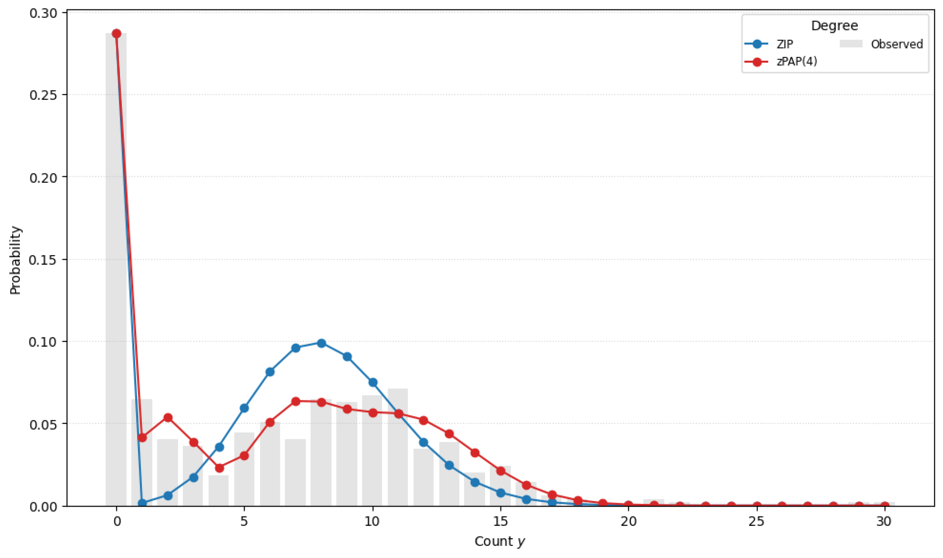
To evaluate the ability of the zPAP model to accommodate both zero-inflation and multimodal count behavior, we augmented the original Fish Catch dataset by superimposing an artificial latent subpopulation. Specifically, an additional set of the same number of observations was drawn from a Poisson distribution with mean $\lambda =10$ and appended to the existing counts. As a result, the combined dataset retains the original zero-inflation while also exhibiting a pronounced secondary mode around 10. Creating this bimodal, zero-inflated dataset is crucial for two reasons: first, it provides a controlled setting in which to assess whether the zPAP model can simultaneously capture excess zeros and a second mass of high counts; second, it mimics real-world scenarios in which heterogeneous subpopulations (e.g., light versus heavy fish catchers) coexist, thereby demonstrating the practical utility of zPAP for complex count data.

Figure 2 overlays the data histogram with each model’s fitted frequencies. The ZIP curve is too narrow—it underestimates overall spread and fails to reproduce the second mode. As we increase the polynomial degree, the zPAP fit rapidly converges to the true distribution, accurately matching both the large spike at zero and the bimodal peaks.

Table 4. MLEs for zero rate, poisson mean, and zero probability.

Model	Zero Rate ($\widehat{\mathit{\pi }}$)	Poisson Mean ($\widehat{\mathit{\lambda }}$)	Predicted $\mathit{p}(\mathit{y}=0)$
Observed	0.2874	5.8806	0.2874
ZIP	0.2873	8.2507	0.2874
zPAP(1)	0.2873	8.2507	0.2874
zPAP(2)	0.2873	8.2507	0.2874
zPAP(3)	0.2843	6.8084	0.2874
zPAP(4)	0.2739	6.1500	0.2875

compares the observed proportion of zero counts in the data with the proportions predicted by each model. As before, the zPAP model provides the closest match, highlighting its capacity to leverage both covariates and the shape of the response distribution. The table presents the estimated Poisson means ($\lambda$), zero-inflation parameters ($\pi$), and the resulting zero probabilities $p(y=0)$ across models of increasing polynomial degree. Although the zero-inflation parameter $\pi$ varies with model complexity, the predicted zero probabilities remain close to the empirical value (≈0.2874). This demonstrates that the zPAP model—particularly at higher degrees—can flexibly adjust both $\lambda$ and the polynomial weights to accurately reproduce the observed zero mass, even under varying internal parameterizations.

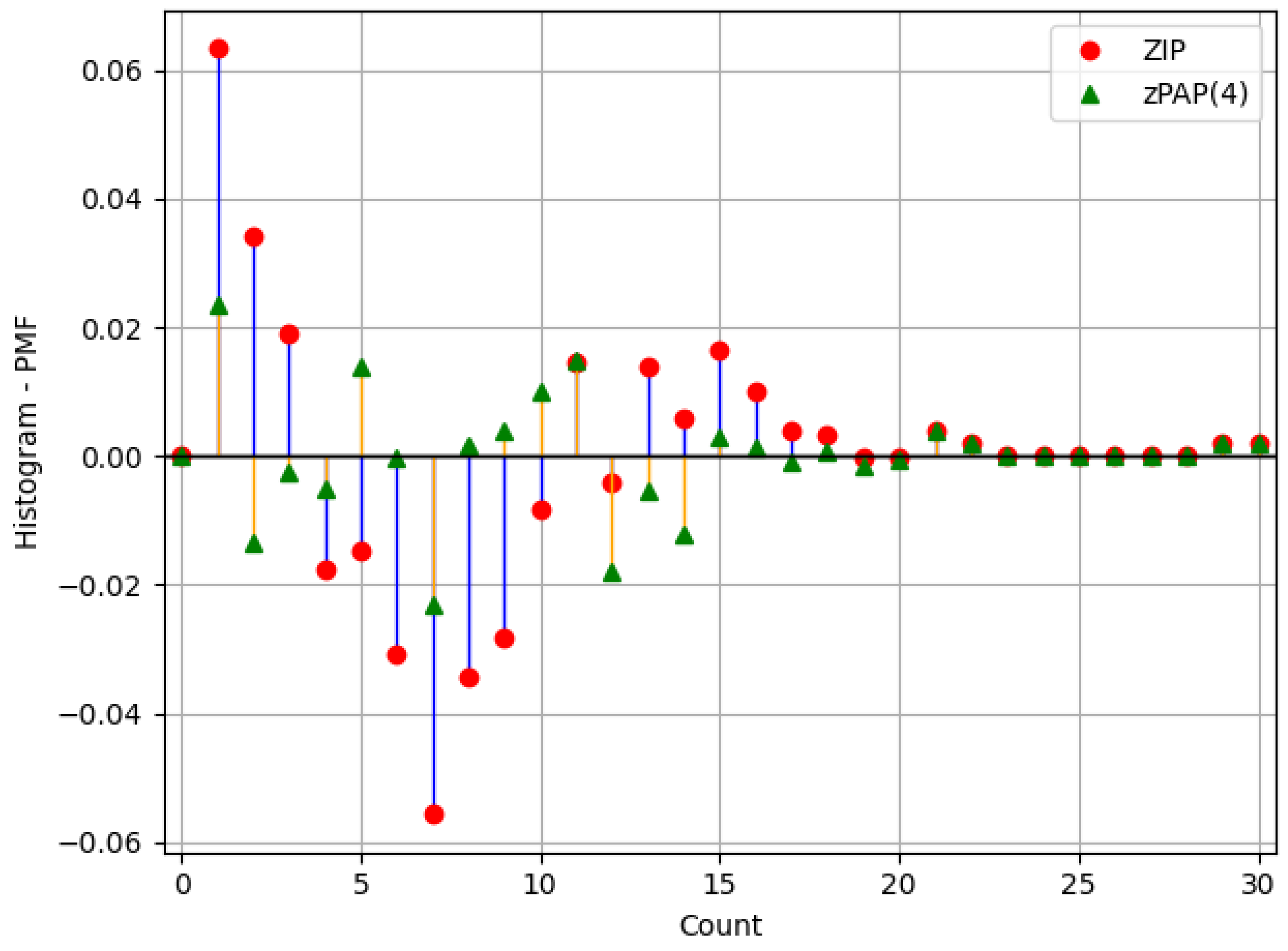
As can be seen in Figure 3, the pointwise differences between the observed PMF and model predictions—ZIP (red dots) and zPAP(4) (green triangles)—demonstrate that the proposed fourth-degree zPAP model substantially reduces discrepancies across the entire range of count values, yielding a more accurate fit to the empirical distribution.

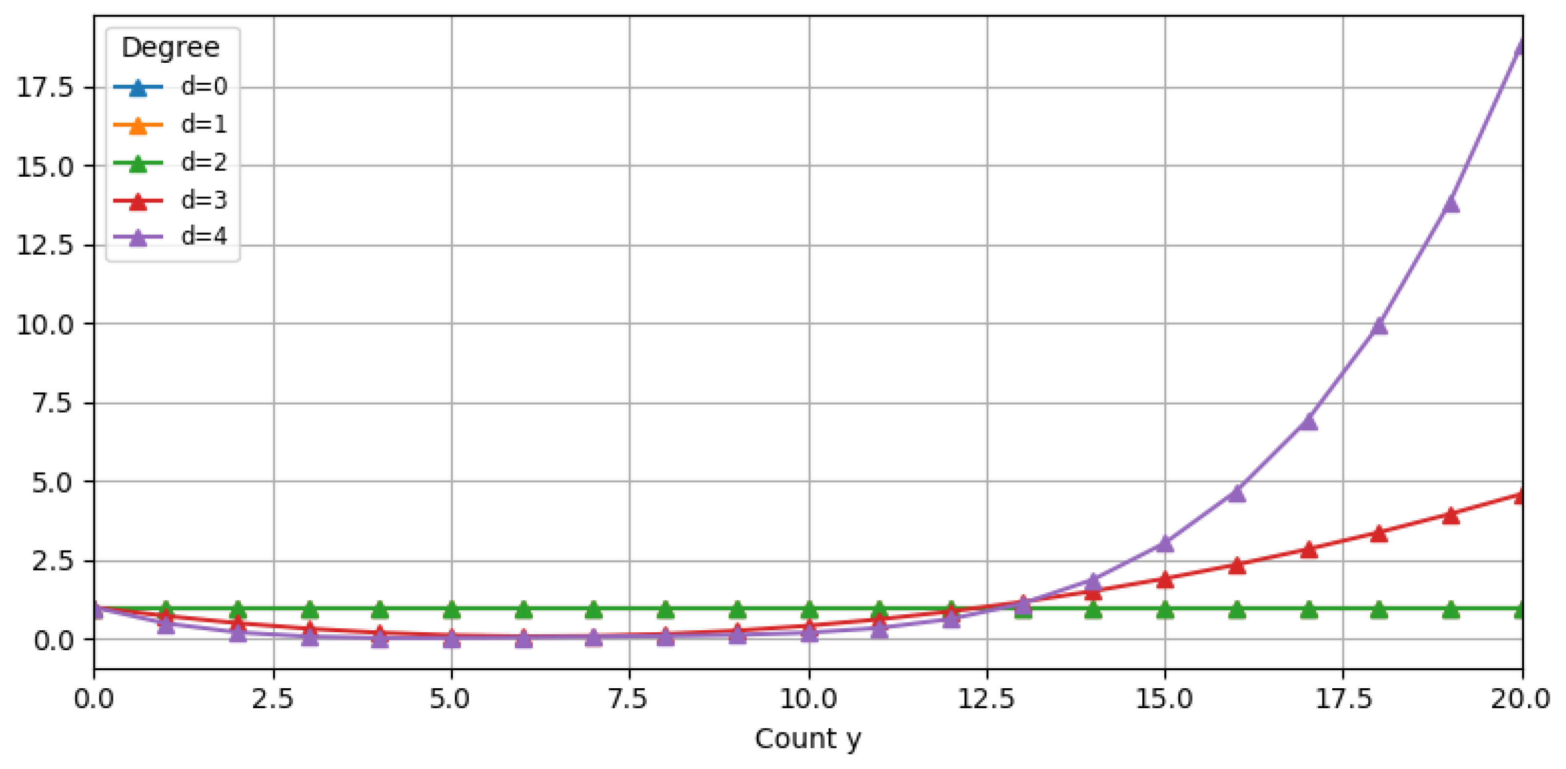
As illustrated in Figure 4, and consistent with the discussion on the convergence of the normalizing constant in Section 2 , the polynomial adjuster $T(y;\alpha )$ grows at most as $O\left(y^d\right)$ as $y\to \infty$. In contrast, Figure 3 shows that the Poisson kernel ${\lambda }^y/y!$ decays super-exponentially, ensuring that the overall model remains stable and capable of capturing heavy-tailed distributions effectively.

5.3. Constructing Bootstrap Confidence Intervals for MLEs

To rigorously assess the uncertainty associated with our MLEs for the proposed zPAP model, one must first establish their large-sample behavior. An analytical derivation of asymptotic properties, namely consistency, asymptotic normality, and efficiency, is mandatory to validate that MLEs converge to the true parameter values and achieve the lower bound of Cramér–Rao. In classical settings, these results follow from regularity conditions on the likelihood and are underpinned by the Fisher information matrix and the observed Hessian of the log-likelihood. However, for the zPAP framework the expressions for the Hessian matrix, the Fisher information matrix, and hence the asymptotic covariance matrix of the MLEs become complex. Closed-form second derivatives of the log-likelihood involve high-dimensional integrals and non-standard functions that preclude straightforward inversion and numerical stability, especially in finite samples.

To overcome these challenges and still provide valid inference on artificial Fish Catch data characterized by zero inflation and bimodal Poisson counts, we employ a parametric bootstrap approach with $B=1000$ replications. Specifically, we generate synthetic datasets by drawing from the fitted zPAP distribution at the estimated parameter values, re-estimate the MLEs for each replicate, and then use the empirical distribution of these bootstrap estimates to form confidence intervals. This procedure not only circumvents the analytical intractability of the model’s Hessian but also delivers accurate finite-sample inference.

We have implemented a parametric bootstrap procedure to compute standard errors, confidence intervals, and the full covariance matrix for the MLEs. By simulating 1000 bootstrap samples, this approach circumvents the analytical intractability of the model’s Hessian matrix and provides more reliable finite-sample inference. To assess the reliability of these intervals, we construct and evaluate coverage probabilities under the assumption of asymptotic normality to ensure that our intervals achieve the intended coverage in practice.

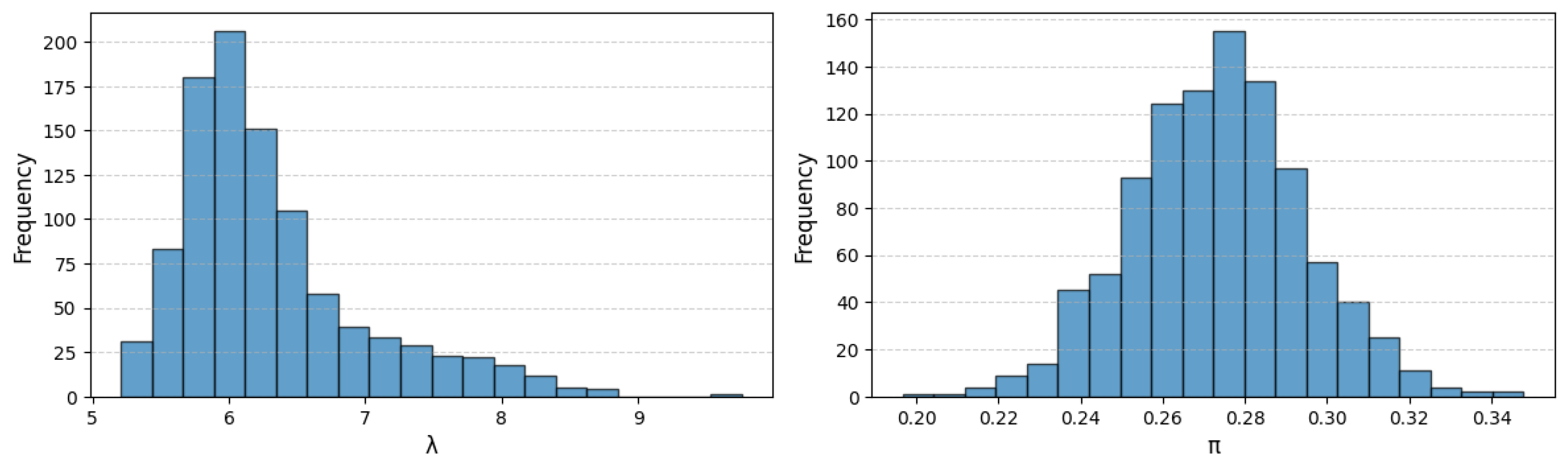
Figure 5 illustrates the bootstrap sampling distributions of the two parameters: in the left panel, the histogram of the Poisson mean $\lambda$ estimates is markedly right-skewed, with a long upper tail indicating occasional larger values, whereas in the right panel the distribution of the zero-inflation probability $\pi$ estimates is symmetric and bell-shaped, closely matching the Gaussian curve expected under asymptotic normality.

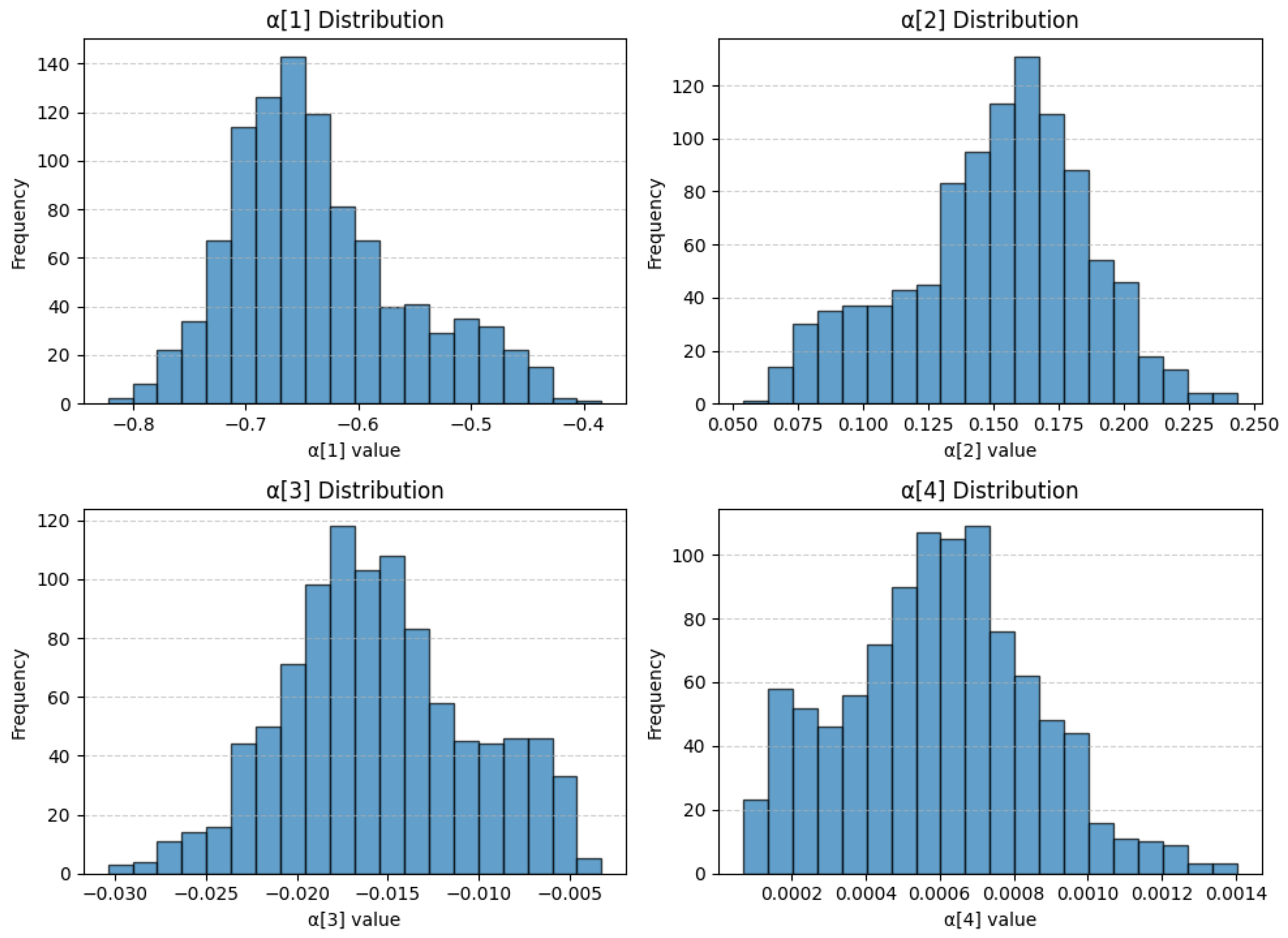
Figure 6 shows the bootstrap sampling distributions of the four degree-4 polynomial adjuster coefficients. While all four distributions are centered around their true values, none are perfectly symmetric. The distribution of ${\alpha }_1$ and ${\alpha }_3$ are noticeably right-skewed, with a pronounced upper tail, whereas ${\alpha }_2$ and ${\alpha }_4$ each exhibit left-skewness, reflected in their longer lower tails.

In

Table 5. Bootstrap summary.

Parameter	Mean	Standard Error	95% Confidence Interval	Coverage Probability
$\lambda$	6.3026	0.6931	[5.4117, 8.1405]	0.933
$\pi$	0.2731	0.0212	[0.2328, 0.3158]	0.950
${\alpha }_1$	−0.6355	0.0779	[−0.7626, −0.4568]	0.934
${\alpha }_2$	0.1510	0.0352	[0.0766, 0.2129]	0.944
${\alpha }_3$	−0.0155	0.0052	[−0.0255, −0.0054]	0.954
${\alpha }_4$	0.0006	0.0003	[0.0001, 0.0011]	0.969

, each column summarizes a different aspect of the bootstrap-derived sampling distribution of the MLEs, all based on $B=1000$ replications. The “Mean” is the average of the B bootstrap estimates for a given parameter. Because the bootstrap draws repeatedly from the fitted model, this empirical average serves not only as a point estimate but also as a simple bias check—if the bootstrap mean differs notably from the original MLE, it suggests small-sample bias. The “Standard Error” is calculated as the sample standard deviation of those B estimates, that is, ${\widehat{\mathrm{SE}}}_{\mathrm{boot}}=\sqrt{{\displaystyle \frac{1}{B-1}}{\sum }_{b=1}^B{\left({\widehat{\theta }}^{*\left(b\right)}-{\overline{\theta }}^{*}\right)}^2},$ and it quantifies the finite-sample variability of the estimator without relying on analytic Hessians or Fisher information.

The 95% confidence interval in the table is constructed by taking the 2.5th and 97.5th percentiles of the sorted bootstrap estimates. For example, for $\lambda$ the interval $[5.4117,8.1405]$ encloses the central 95% of the ${\widehat{\lambda }}^{*}$ values. This percentile method implicitly accounts for skewness in the bootstrap distribution, so that asymmetric intervals arise naturally when the sampling distribution is skewed.

Under the asymptotic-normality assumption, each 95% interval is formed as ${\widehat{\theta }}_{\mathrm{mean}}\pm 1.96{\widehat{\mathrm{SE}}}_{\mathrm{boot}}.$ Table 5 shows that these intervals achieve coverage probabilities very close to the nominal 95% level: $\pi$ hits exactly 0.950, ${\alpha }_3$ comes in at 0.954, and ${\alpha }_2$ at 0.944. The scale parameter $\lambda$ exhibits slight under-coverage (0.933), while the highest-order coefficient ${\alpha }_4$ is slightly conservative (0.969), reflecting its very small variance and the corresponding tail behavior of its bootstrap distribution.

$$\mathsf{\Sigma }=\begin{array}{cc}& \begin{array}{cccccc}\lambda & \pi & {\alpha }_1& {\alpha }_2& {\alpha }_3& {\alpha }_4\end{array}\\ \begin{array}{}\lambda & \pi & {\alpha }_1& {\alpha }_2& {\alpha }_3& {\alpha }_4\end{array}& \left(\begin{array}{cccccc}0.48039411& 0.00351852& 0.05192662& -0.02312406& 0.00335162& -0.00016195\\ 0.00351852& 0.00044764& 0.00039592& -0.00017702& 0.00002578& -0.00000125\\ 0.05192662& 0.00039592& 0.00607207& -0.00272718& 0.00039795& -0.00001929\\ -0.02312406& -0.00017702& -0.00272718& 0.00123572& -0.00018180& 0.00000888\\ 0.00335162& 0.00002578& 0.00039795& -0.00018180& 0.00002696& -0.00000133\\ -0.00016195& -0.00000125& -0.00001929& 0.00000888& -0.00000133& 0.00000007\end{array}\right)\end{array}$$

The matrix $\mathsf{\Sigma }$ is the empirical covariance of the bootstrap estimates for all six parameters, with rows and columns ordered as $\{\lambda ,\pi ,{\alpha }_1,{\alpha }_2,{\alpha }_3,{\alpha }_4\}$. Each diagonal entry gives the bootstrap variance of that parameter (for example, $\mathrm{Var}\left({\widehat{\lambda }}^{*}\right)=0.4804$ and $\mathrm{Var}\left({\widehat{\pi }}^{*}\right)=0.0004476$), which correspond to the squared standard errors reported in Table 5. The much larger variance for $\lambda$ compared to $\pi$ reflects greater sampling variability in the scale parameter under our model. Off-diagonal entries capture pairwise covariances. A positive covariance, such as $\mathrm{Cov}({\widehat{\lambda }}^{*},{\widehat{\alpha }}_1^{*})=0.0519$, indicates that bootstrap draws in which $\lambda$ is higher than its mean tend also to have larger ${\alpha }_1$. Conversely, the negative covariance between $\lambda$ and ${\alpha }_2$ ($-0.0231$) shows that when $\lambda$ is relatively large, ${\alpha }_2$ tends to be smaller. The tiny covariances involving ${\alpha }_4$ are consistent with its very small variance (0.00000007), indicating that ${\alpha }_4$ is estimated with high precision and almost independently of the other coefficients.

6. Concluding Remarks

We introduced the zero-inflated Polynomially Adjusted Poisson (zPAP) model. It extends the usual zero-inflated Poisson to handle extra zeros, overdispersion, skewness, and even bimodal counts. The key idea is to multiply the Poisson kernel by a simple polynomial weight, while still using a logistic link for zero inflation.

In the main text, we gave the full mathematical setup. We wrote down the adjusted likelihood and showed how each parameter—zero-inflation probability $\pi$, Poisson rate $\lambda$, and polynomial coefficients $\alpha$—can depend on covariates. We then derived the maximum-likelihood equations and explained how to compute them in practice. That discussion covers how to pick starting values, enforce identifiability constraints, and evaluate the normalizing constant and its derivatives. By spelling out the log-likelihood and score functions, we give both the theory and a clear recipe for implementation.

We tested the zPAP model on two datasets. First, we used the Fish Catch data, which has many zeros and high dispersion. Then, we created a mixed dataset by adding random Poisson counts to the Fish Catch observations, producing a clear bimodal pattern. In both cases, zPAP fit the data better than the standard ZIP model, handling multiple peaks and skewed shapes with ease. We generated 1000 bootstrap datasets by sampling from the fitted zPAP(4) model, re-estimating the MLEs on each replicate, and used the resulting estimate distributions to compute standard errors, confidence intervals, and the covariance matrix.

In summary, zPAP is a powerful yet interpretable extension of classical count models. It can flexibly capture a wide range of patterns in count data. Future work will first establish the large-sample properties of the zPAP maximum-likelihood estimators—proving consistency, asymptotic normality, and efficiency under standard regularity conditions. We will also investigate using an orthogonal polynomial basis for $T(y;\alpha )$ to improve numerical stability and interpretability. In addition, we plan to compare different fitting methods—such as the method of moments and least squares—against maximum likelihood to see how they perform in practice.