A Quantile Spillover-Driven Markov Switching Model for Volatility Forecasting: Evidence from the Cryptocurrency Market

Abstract

This paper develops a novel modeling framework that integrates time-varying quantile-based spillover effects into a regime-switching realized volatility model. A dynamic spillover factor is constructed by identifying the most influential contributors to Bitcoin’s realized volatility across different quantile levels. This quantile-layered structure enables the model to capture heterogeneous spillover paths under varying market conditions at a macro level while also enhancing the sensitivity of volatility regime identification via its incorporation into a time-varying transition probability (TVTP) Markov-switching mechanism at a micro level. Empirical results based on the cryptocurrency market demonstrate the superior forecasting performance of the proposed TVTP-MS-HAR model relative to standard benchmark models. The model exhibits strong capability in identifying state-dependent spillovers and capturing nonlinear market dynamics. The findings further reveal an asymmetric dual-tail amplification and time-varying interconnectedness in the spillover effects, along with a pronounced asymmetry between market capitalization and systemic importance. Compared to decomposition-based approaches, the X-RV type of models—especially when combined with the proposed quantile-driven factor—offers improved robustness and predictive accuracy in the presence of extreme market behavior. This paper offers a coherent approach that bridges phenomenon identification, source localization, and predictive mechanism construction, contributing to both the academic understanding and practical risk assessment of cryptocurrency markets.

1. Introduction

Against the backdrop of profound adjustments in the global economic landscape and frequent structural shocks—such as the COVID-19 pandemic, geopolitical tensions, and unconventional monetary policy expansions—cryptocurrencies have increasingly been regarded by investors as emerging assets for hedging traditional financial market risks. Owing to their low correlation with traditional financial assets [1], cryptocurrencies are increasingly viewed as highly speculative financial instruments. Since the advent of Bitcoin in 2009, the market capitalization of cryptocurrencies has reached several trillion US dollars by 2019 [2], with Bitcoin and Ethereum constituting the core structure [3].

Compared to traditional financial markets, the cryptocurrency market exhibits significant differences in structural and behavioral characteristics, mainly reflected in three aspects: (1) its 24/7 trading mechanism, highly heterogeneous investor structure, and pronounced sentiment-driven behavior result in volatility clustering that is much stronger than in traditional markets; (2) the absence of a central clearing mechanism makes risk propagation more dependent on the market’s network structure, leading to more complex nonlinear spillover paths; (3) a retail investor-dominated market structure amplifies sentiment-driven fluctuations, causing more pronounced asymmetric spillover effects.

Due to these features, the cryptocurrency market not only experiences extreme volatility more frequently [4] but the high interconnectedness among assets [5,6] also facilitates the evolution of localized shocks into systemic risks that rapidly spread throughout the market. This complex nonlinear dynamic, jointly driven by internal linkage mechanisms and external shocks, coupled with fundamental differences from traditional markets at the microstructural level [7], underscores the necessity of precisely modeling realized volatility ($RV$) in cryptocurrencies [8], which is crucial for risk management and market stability assessment.

Existing studies indicate that the cryptocurrency market is highly isolated at the systemic level from traditional financial markets. For example, Manavi et al. [9] employed correlation matrices and hierarchical clustering to reveal that crypto-assets form a distinct cluster characterized by more intense internal volatility and fundamentally different driving logic and intrinsic linkages compared to fiat currencies, commodities, and major financial indices. This phenomenon stems not only from external shocks but also from the market’s inherent structure [7]. Empirical research by Corbet et al. [10] and Ciaian et al. [11] further confirms that the extreme volatility of cryptocurrencies is not entirely driven by speculative behavior but is endogenous to a highly interlinked ecosystem, reflecting the deep coupling of technology, network structure, and market mechanisms.

Traditional time series models, such as the Autoregressive Conditional Heteroskedasticity (ARCH) model proposed by Engle [12] and its extension, the Generalized ARCH (GARCH) model by Bollerslev [13], laid the foundation for capturing the volatility characteristics of financial time series. Several studies, including Chu et al. [14] and Katsiampa [15], investigated the accuracy of various GARCH-type models in forecasting the realized volatility of the cryptocurrency market. However, the application of GARCH-type models in this context is inherently limited. Their entire design philosophy and statistical assumptions are based on low-frequency data, making it difficult for them to directly leverage high-frequency data to capture intraday volatility patterns. The information revolution brought by high-frequency data has spurred the development of a new generation of more suitable and direct volatility models, such as the HAR model. For instance, Hoang and Baur [16] applied the Heterogeneous Autoregressive Model of Realized Volatility (HAR-RV) [17] to forecast Bitcoin volatility. With its parsimonious structure and outstanding predictive performance, the HAR-RV has become a benchmark model in the field of realized volatility forecasting. In recent years, to further enhance its explanatory power and predictive accuracy, scholars have extended the classic HAR-RV model in various dimensions. For example, by incorporating jump components [18] or integrating realized semi-variance [19], these extensions have improved the explanatory power and forecasting precision of the HAR type, demonstrating the flexibility and extensibility of its framework.

Empirical studies have shown that the cryptocurrency market is influenced by factors such as business cycle fluctuations, unexpected shocks, and policy interventions [20]. As a result, the statistical properties of volatility—such as its persistence—often exhibit structural breaks [21] or significant regime-switching behavior [22], typically manifested as alternations between high- and low-volatility states.

Building on this foundation, Raggi and Bordignon [23] integrated the regime-switching mechanism with the ARIMA model characterized by long-memory properties [24], aiming to capture both short-term regime changes and long-term dependency structures. By incorporating state-dependent parameters, this approach significantly enriched the model’s dynamic behavior. However, its applicability under high-dimensional data settings or extreme volatility conditions is constrained due to computational complexity and the stability of parameter estimation—particularly in high-frequency financial markets, where its performance may fall short of expectations. To better address the characteristics of high-frequency financial data, Ma et al. [25] embedded the regime-switching mechanism into the Heterogeneous Autoregressive (HAR) framework, proposing a predictive model tailored to realized volatility ($RV$). The HAR model has gained widespread recognition for its ability to capture volatility across multiple time horizons [26]. With the addition of regime switching, the model becomes more adaptive to dynamic changes in market conditions, such as transitions between high- and low-volatility regimes. Empirical results from Ma et al. [25] demonstrate that this method significantly improves volatility forecasting accuracy in equity markets, especially during periods of intense market turbulence. However, the study’s main limitation lies in its relatively simplistic modeling of regime transition probabilities, which does not adequately account for the potential influence of exogenous variables, thereby limiting the model’s generalizability in more complex market environments.

In the emerging field of cryptocurrency markets, the extreme nature and nonlinear characteristics of volatility pose greater challenges for traditional models in forecasting. Addressing the unique volatility dynamics in this context, Ma et al. [27] innovatively incorporated exogenous variables into the regime-switching framework, extending the regime transition probability modeling approach proposed by Diebold et al. [28]. By dynamically modeling transition probabilities using external variables such as market liquidity and trading volume, their approach significantly enhanced the model’s flexibility and accuracy in forecasting cryptocurrency volatility. For instance, the study found that fluctuations in trading volume and market sentiment can substantially influence the duration of high-volatility regimes—offering new insights into the microstructure of cryptocurrency markets. Nevertheless, while the method performs well in capturing short-term volatility patterns, its capacity to forecast long-term trends remains limited due to the incomplete selection and varying quality of exogenous variables. Moreover, the robustness of Ma et al. [27] model under extreme market conditions—such as cryptocurrency crashes—has not been fully validated, potentially limiting its practical applicability in real-world investment decisions.

In contrast, other studies offer alternative perspectives on cryptocurrency volatility forecasting. For example, Bildirici and Ersin [29] proposed a regime-switching model based on fractional integration to capture the long-memory properties of cryptocurrency markets; however, the model’s high computational complexity hinders its applicability in real-time forecasting. Similarly, Nooijen and Broda [30] explored a GARCH-based regime-switching approach that emphasizes the role of sentiment indicators in volatility prediction, but its reliance on a subjectively pre-specified number of regimes may introduce the risk of overfitting. Compared to these approaches, the key contribution of Ma et al. [27] lies in the dynamic modeling of regime transition probabilities through exogenous variables, offering a more flexible mechanism for capturing the nonlinear dynamics of cryptocurrency markets. However, limitations in the model’s ability to forecast long-term trends and validate robustness under extreme market events remain areas that require further improvement.

Although the aforementioned studies have provided valuable insights into the drivers of volatility regime shifts from the perspectives of macroeconomic indicators [31] and specific exogenous shocks [32], the influence of dynamic factors rooted in the internal structural features of the market has not been sufficiently explored—particularly in the context of cryptocurrency markets characterized by high market interconnectedness and real-time information transmission. In particular, the critical role of cross-asset volatility spillover effects in regime-switching processes has yet to be systematically examined from both theoretical and empirical perspectives. The high degree of interconnection within cryptocurrency markets means that volatility in major assets (such as Bitcoin and Ethereum) can rapidly affect other assets through price co-movements, trading volume correlations, or the diffusion of market sentiment, potentially triggering transitions in the overall market volatility regime. However, the existing literature predominantly focuses on modeling the volatility of individual assets, paying limited attention to how cross-asset volatility spillovers dynamically influence regime transition probabilities and the associated micro-level mechanisms (such as order book depth or liquidity shocks). This gap not only limits our comprehensive understanding of the complex volatility mechanisms in cryptocurrency markets but may also undermine the predictive power of regime-switching models during extreme market events—such as crashes or rapid rebounds.

To fill this research gap, the role of cross-asset volatility spillover effects warrants deeper investigation. For example, the study by Diebold and Yilmaz [33] offers important insights into internal market volatility spillovers. They found that volatility transmission among assets within the market is not only a key external driver of overall volatility but may also serve as a trigger or moderator of volatility regime switches. Specifically, when the market is exposed to significant positive or negative spillover shocks, this intense market resonance can lead to abrupt transitions from low- to high-volatility regimes, and vice versa. This finding provides a new perspective for modeling volatility in cryptocurrency markets, suggesting that further research should investigate how cross-asset volatility spillovers dynamically influence regime transition probabilities through mechanisms embedded in the market microstructure.

Building upon the above discussion, this paper proposes an innovative volatility forecasting model that incorporates dynamic regime switching driven by spillover effects. This model advances the traditional HAR framework in two key ways. First, by analyzing the Total Spillover Index (TSI), it captures the overall interconnectedness of the cryptocurrency system, demonstrating that the transmission of shocks is both time-varying and regime-dependent. Second, by decomposing the Net Spillover Index (NSI), the model identifies which cryptocurrencies act as dominant transmitters or recipients of volatility across different market states, thereby revealing the hierarchical structure and role-switching dynamics within the spillover network. Furthermore, the model focuses on the pairwise spillover effects on Bitcoin, enabling the precise identification of the most influential driver cryptocurrencies across different quantiles. This new approach provides a more accurate representation of volatility regime transitions triggered by internal information flows and sentiment contagion, thereby deepening our understanding of the complex dynamics in cryptocurrency markets and enhancing the predictive power of regime-dependent volatility models.

The objectives and marginal contributions of this paper are threefold. Theoretically, it establishes two key empirical facts regarding risk transmission in cryptocurrency markets: (1) the coexistence of asymmetric dual-tail amplification effects in spillovers and path-dependent asymmetries between downside and upside risks and (2) a structural asymmetry between market capitalization and systemic influence, where systemic importance is determined by functional centrality, rather than mere market size, thereby correcting a common misperception. Methodologically, this study proposes a novel quantile-driven spillover factor, which distills complex and time-varying network structures into an economically interpretable, endogenous driver capable of explaining volatility regime transitions. This factor is further embedded within a Time-Varying Transition Probability Markov-Switching Heterogeneous Autoregressive (TVTP-MS-HAR) model, and empirical results show that it significantly improves forecasting accuracy compared to all benchmark models. (3) Empirically, the paper demonstrates that the X-RV type model, which aggregates realized volatility, offers a robust tool for handling the chaotic nature of cryptocurrency markets, better identifying regime-specific spillovers and capturing nonlinear dynamics. Overall, this study provides deeper insights and a more effective analytical framework for understanding and forecasting volatility in highly interconnected and complex financial systems.

The remainder of this paper is organized as follows. Section 2 reviews the fundamental theories of volatility and quantile spillovers. Section 3 introduces all the baseline models used in this study and the methodology for constructing the combined models. Subsequently, Section 4 empirically investigates the spillover effects in the cryptocurrency market. Section 5 presents the empirical analysis; this paper evaluates the forecasting performance of the FTP-HAR and TVTP-HAR model families using various statistical tests, including the Model Confidence Set (MCS) test [34] and the out-of-sample $R^2$ statistic [35]. This paper then reports and discusses the results. Finally, Section 6 concludes the paper, highlighting that our proposed TVTP-MS-HAR model demonstrates a superior predictive ability.

2. Theoretical Analysis

2.1. Time-Varying Quantile Spillover Theory

A core challenge in studying risk transmission across financial markets lies in capturing the nonlinear and time-varying nature of systemic interconnectedness. Traditional linear models, such as the standard VAR, or time-varying models that focus solely on conditional means, implicitly assume that the propagation mechanism of shocks remains stable over time and across different market states. However, both empirical evidence and financial practice suggest that market behavior in the tails significantly deviates from normal conditions. For instance, during crisis periods, the transmission of bad news tends to be faster and broader, a phenomenon commonly referred to as asymmetric spillover.

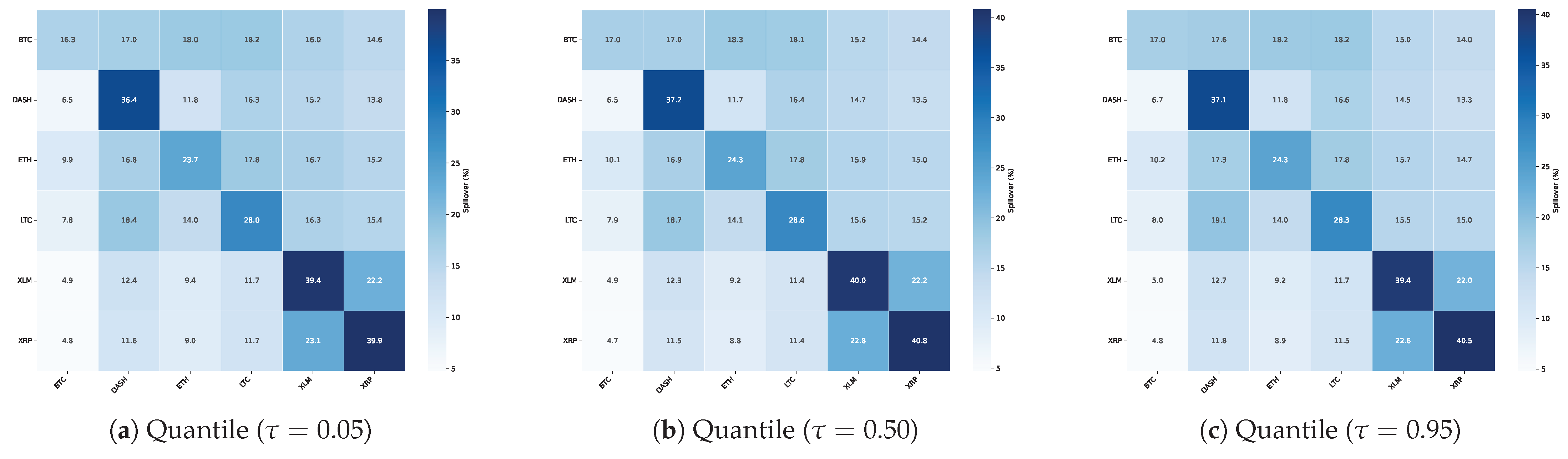
To better characterize such state- and time-dependent connectedness, a comprehensive framework based on time-varying quantile spillovers (TVQs) is developed. This approach facilitates a slice-wise decomposition of spillover effects across various quantile levels ($\tau$), capturing market conditions that range from extremely pessimistic to extremely optimistic. In addition, it allows for the dynamic monitoring of how these spillover patterns evolve over time. Following the methodologies proposed by Zhang and Ma [36], Bouri et al. [37], Jena et al. [38], and Gong et al. [39], the time-varying quantile spillover model is constructed as follows. The Time-Varying Parameter Quantile Vector Autoregressive (TVP-QVAR) model extends the conventional static-coefficient framework to a dynamic, time-varying specification:

$$y_t=c_t\left(\tau \right)+\sum _{i=1}^p{B}_{i,t}\left(\tau \right)y_{t-i}+u_t\left(\tau \right),$$

(1)

where $y_t$ is an $n\times 1$ vector of market returns, $c_t\left(\tau \right)$ is the time-varying intercept vector, and $B_{i,t}\left(\tau \right)$ are the time-varying autoregressive coefficient matrices. The error structure, characterized by the innovation term $u_t\left(\tau \right)$ and its time-varying covariance matrix ${\mathsf{\Sigma }}_{u,t}\left(\tau \right)$, is also a function of the target quantile $\tau \in (0,1)$. This design allows the model to flexibly adapt to different market conditions: when $\tau$ is set to the median (0.5), the model describes normal market behavior, whereas, when $\tau$ approaches the tails (0 or 1), it focuses on the market’s tail dynamics under extreme negative or positive shocks, respectively. To facilitate estimation and compact representation, we define the stacked coefficient matrix as $B_t\left(\tau \right)=\left[B_{1,t}\left(\tau \right),B_{2,t}\left(\tau \right),\dots ,B_{p,t}\left(\tau \right)\right]$. To model the evolution of the time-varying parameters, they are typically assumed to follow a random walk process:

$$\begin{array}{cc}\hfill \mathrm{vec}\left(B_t\left(\tau \right)\right)& =\mathrm{vec}\left(B_{t-1}\left(\tau \right)\right)+v_{B,t}\left(\tau \right),\hfill \end{array}$$

(2)

$$\begin{array}{cc}\hfill c_t\left(\tau \right)& =c_{t-1}\left(\tau \right)+v_{c,t}\left(\tau \right).\hfill \end{array}$$

(3)

where $B_t\left(\tau \right)$ is the stacked form of all lagged coefficient matrices, $\mathrm{vec}(·)$ is the vectorization operator, and $v_{B,t}\left(\tau \right)$ and $v_{c,t}\left(\tau \right)$ are Gaussian white noise innovations. This specification endows the model with considerable flexibility, enabling it to capture the smooth evolution of shock transmission paths over time (indexed by t) under different market states (determined by $\tau \in (0,1)$).

For the estimation of this model, instead of employing computationally intensive Bayesian MCMC methods, this paper adopts the widely used adaptive estimation paradigm from Antonakakis et al. [40]. The core of this method lies in the combination of the Kalman filter with forgetting factors.

Equation (1) is first cast into a state-space form. All time-varying coefficients are stacked into a single state vector, ${\beta }_t\left(\tau \right)$:

$${\beta }_t\left(\tau \right)=\mathrm{vec}\left([c_t\left(\tau \right),B_{1,t}\left(\tau \right),\dots ,B_{p,t}\left(\tau \right)]\right).$$

(4)

The state equation, which governs the evolution of the parameters, assumes a random walk:

$${\beta }_t\left(\tau \right)={\beta }_{t-1}\left(\tau \right)+v_t\left(\tau \right),v_t\left(\tau \right)\sim \mathcal{N}(0,Q),$$

(5)

where Q is the covariance matrix of the state disturbances, $v_t\left(\tau \right)$.

The measurement equation links the observable data, $y_t$, to the unobserved state vector:

$$y_t=X_t^{\prime }{\beta }_t\left(\tau \right)+u_t\left(\tau \right),u_t\left(\tau \right)\sim \mathcal{N}(0,{\mathsf{\Sigma }}_{u,t}\left(\tau \right)),$$

(6)

where $X_t=I_n\otimes [1,y_{t-1}^{\prime },\dots ,y_{t-p}^{\prime }]$ is the matrix of explanatory variables, including the intercept and lagged values of $y_t$, and ⊗ denotes the Kronecker product. In practice, the model is estimated using a recursive forward pass of the Kalman filter. To allow the model to adapt to structural changes, the error covariance matrix, ${\mathsf{\Sigma }}_{u,t}\left(\tau \right)$, and the state covariance matrix, Q, are updated adaptively using forgetting factors. For instance, the time-varying error covariance matrix is updated as follows:

$${\mathsf{\Sigma }}_{u,t}\left(\tau \right)=\lambda {\mathsf{\Sigma }}_{u,t-1}\left(\tau \right)+(1-\lambda )u_{t-1}\left(\tau \right)u_{t-1}{\left(\tau \right)}^{\prime },$$

(7)

where the forgetting factor $\lambda \in (0,1)$ controls the extent to which the model relies on past information. A value of $\lambda$ close to 1 implies smoother parameter changes, whereas a lower value makes the model more responsive to recent information. This approach yields a unique set of parameter estimates, $({\widehat{\beta }}_t\left(\tau \right),{\widehat{\mathsf{\Sigma }}}_{u,t}\left(\tau \right))$, for each point in time t through a forward recursion.

Based on the time-varying parameter estimates ${\widehat{\beta }}_t\left(\tau \right)$ and ${\widehat{\mathsf{\Sigma }}}_{u,t}\left(\tau \right)$ obtained at each time point t, the corresponding time-varying impulse response functions (IRFs), denoted as $A_{h,t}\left(\tau \right)$, can be derived. Subsequently, the Generalized Forecast Error Variance Decomposition (GFEVD) framework proposed by Pesaran and Shin [41] is employed to quantify spillover effects. Within the quantile framework, the contribution of a shock in variable j to the H-step forecast error variance of variable i at time t, denoted by ${\varphi }_{ij,t}^g(H,\tau )$, is calculated as follows:

$${\varphi }_{ij,t}^g(H,\tau )={\displaystyle \frac{{\sigma }_{jj,t}^{-1}\left(\tau \right){\sum }_{h=0}^{H-1}{\left(e_i^{\prime }{A}_{h,t}\left(\tau \right){\mathsf{\Sigma }}_{u,t}\left(\tau \right)e_j\right)}^2}{{\sum }_{h=0}^{H-1}{e}_i^{\prime }{A}_{h,t}\left(\tau \right){\mathsf{\Sigma }}_{u,t}\left(\tau \right)A_{h,t}{\left(\tau \right)}^{\prime }{e}_i}}.$$

(8)

where ${\sigma }_{jj,t}\left(\tau \right)$ is the $(j,j)$-th element of the time-varying covariance matrix ${\mathsf{\Sigma }}_{u,t}\left(\tau \right)$, and $e_j$ is a selection vector with unity for the j-th element and zeros otherwise.

To facilitate interpretation and the construction of spillover indices, each row of the GFEVD matrix is normalized so that its elements sum to one:

$${\tilde{\varphi }}_{ij,t}^g(H,\tau )={\displaystyle \frac{{\varphi }_{ij,t}^g(H,\tau )}{{\sum }_{j=1}^n{\varphi }_{ij,t}^g(H,\tau )}}.$$

(9)

This yields a time-varying $n\times n$ normalized spillover matrix, ${\tilde{\mathsf{\Phi }}}_t^g(H,\tau )=\left[{\tilde{\varphi }}_{ij,t}^g(H,\tau )\right]$. The matrix ${\tilde{\mathsf{\Phi }}}_t^g(H,\tau )$ precisely represents the contribution of variable j to the future volatility of variable i at quantile $\tau$ and time t, serving as the direct input for constructing our spillover index system.

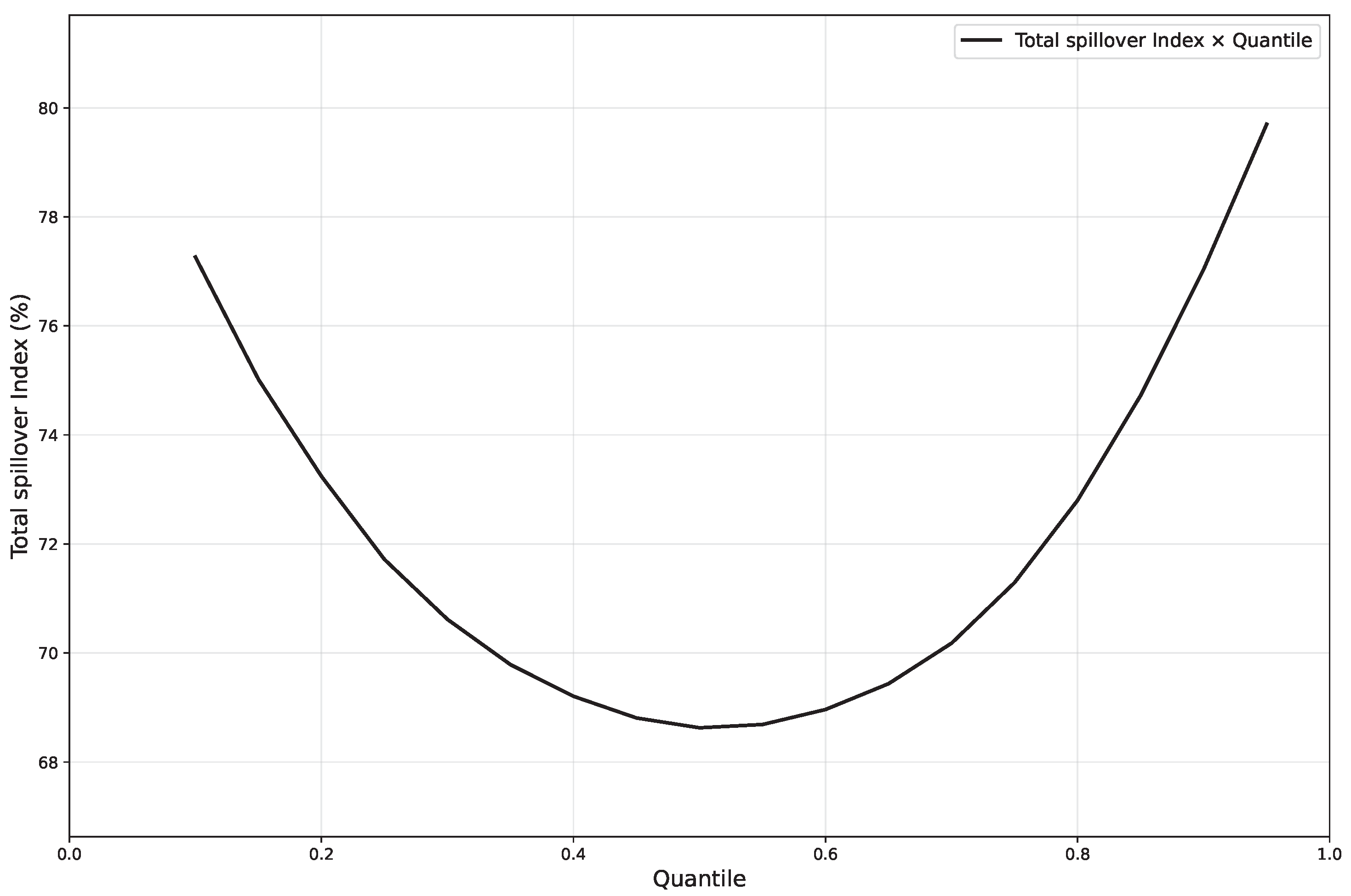
Based on this normalized quantile variance decomposition matrix, a multi-layered spillover index system, from macro to micro levels, can be constructed. First, at the macro level, the total spillover index measures the overall intensity of cross-variable influences within the system and can be seen as a comprehensive metric of systemic connectedness:

$${\mathrm{TSI}}_t(H,\tau )={\displaystyle \frac{{\sum }_{i=1}^n{\sum }_{\begin{array}{c}j=1,j\ne i\end{array}}^n{\tilde{\varphi }}_{ij,t}^g(H,\tau )}{n}}\times 100.$$

(10)

Second, to identify the main sources and destinations of spillovers within the network, the total spillover can be further decomposed into directional spillovers. Specifically, the total spillover transmitted from market i to all other markets and the total spillover received by market i from all other markets are defined, respectively, as follows:

$$S_{·\leftarrow i,t}(H,\tau )=\sum _{j=1,j\ne i}^n{\tilde{\varphi }}_{ji,t}^g(H,\tau ),$$

(11)

$$S_{i\leftarrow ·,t}(H,\tau )=\sum _{j=1,j\ne i}^n{\tilde{\varphi }}_{ij,t}^g(H,\tau ).$$

(12)

Finally, the net directional spillover for each market can be computed.

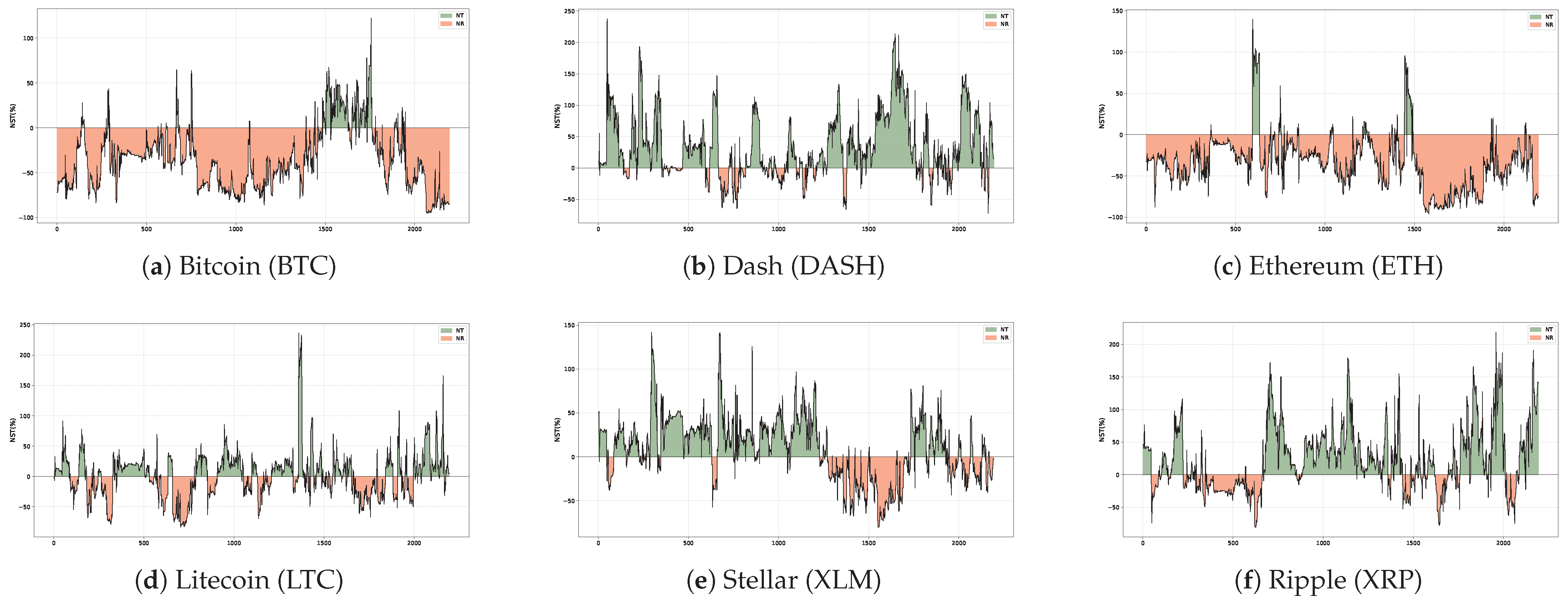
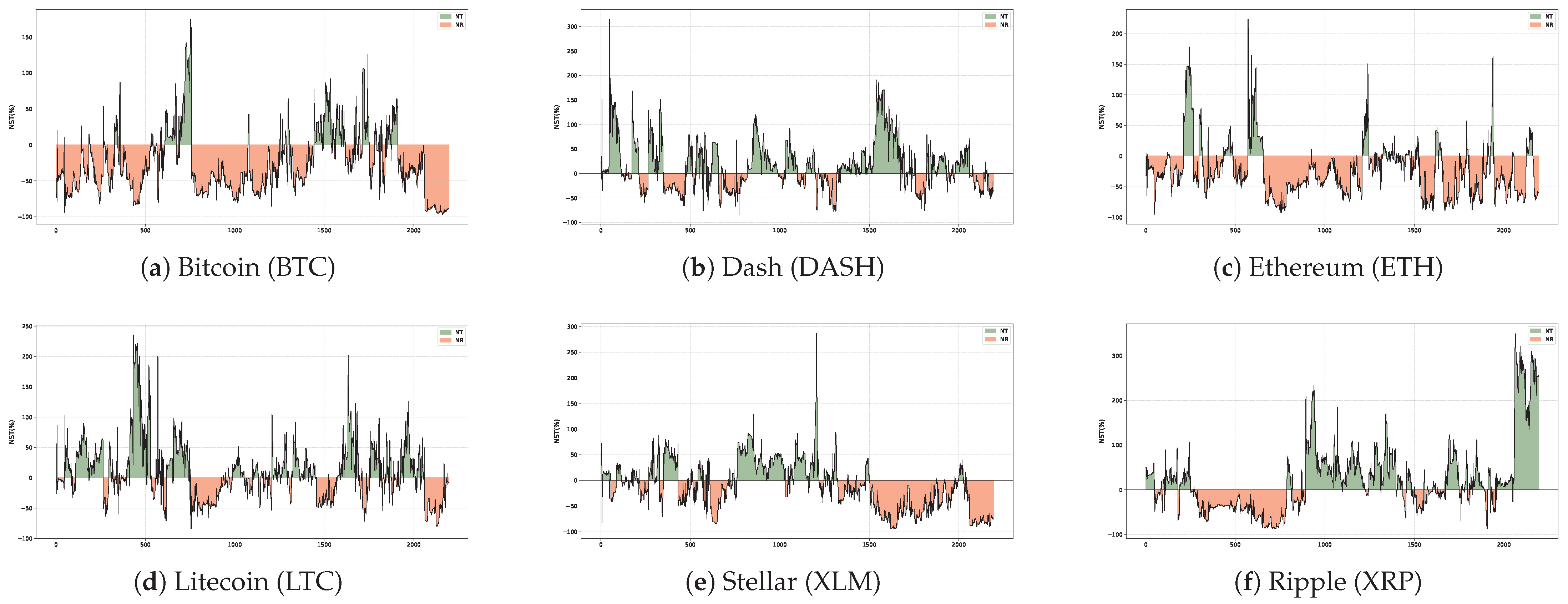
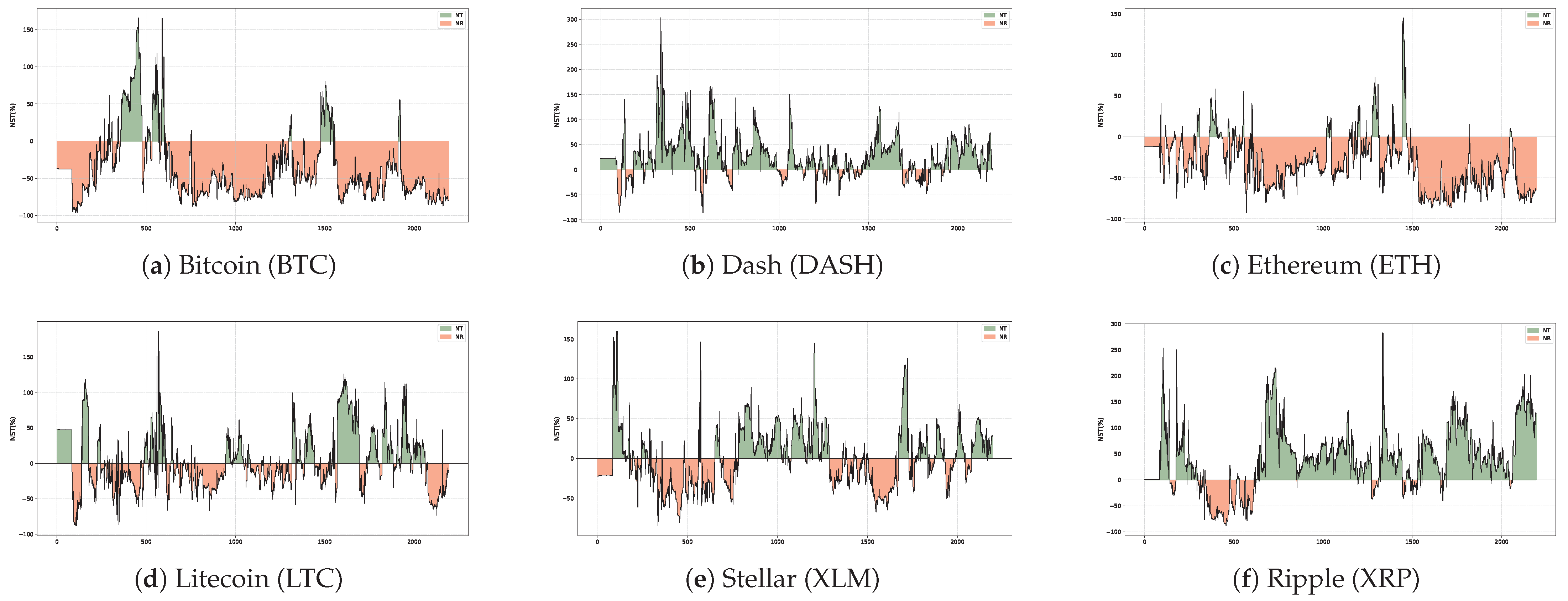
Dynamic Net Spillover Index (NSI): This index quantifies the net spillover contribution of an individual market to the entire system at a specific time and under a given market state. It is calculated as the difference between the gross spillovers transmitted to and received from all other markets:

$$S_{i,\mathrm{net},t}(H,\tau )=S_{·\leftarrow i,t}(H,\tau )-S_{i\leftarrow ·,t}(H,\tau ).$$

(13)

A positive value of $S_{i,\mathrm{net},t}(H,\tau )$ indicates that market i is a net transmitter of spillovers, contributing more to the system than it absorbs. Conversely, a negative value suggests that market i is a net receiver, whose volatility is more susceptible to systemic shocks from external sources. The time series of this index reveals the dynamic role-switching of a market across different periods.

Net Pairwise Directional Connectedness (NPDC): This index measures the net spillover effect between any two specific markets, i and j:

$${\mathrm{NPDC}}_{j\to i,t}(H,\tau )=\left({\tilde{\varphi }}_{ij,t}^g(H,\tau )-{\tilde{\varphi }}_{ji,t}^g(H,\tau )\right)\times 100.$$

(14)

The spillover index system constructed above provides the foundation for quantifying the complex linkages within the cryptocurrency network. The central objective of this paper is to leverage this granular network information to select the most effective driving variables for our realized volatility forecasting models. Traditional approaches often select a fixed asset as the driver, overlooking the fact that the primary source of influence can shift across different market environments. To overcome this limitation, this paper proposes a dynamic and composite driving variable selection strategy.

The core idea of this strategy is that forecasting the realized volatility of a target asset, i, should not rely solely on the effects observed under normal market conditions. Instead, it is crucial to identify, across different market states—including high-volatility, low-volatility, and tranquil periods—the key cryptocurrency, j, that exerts the most significant spillover effect on asset i.

The specific implementation steps are as follows:

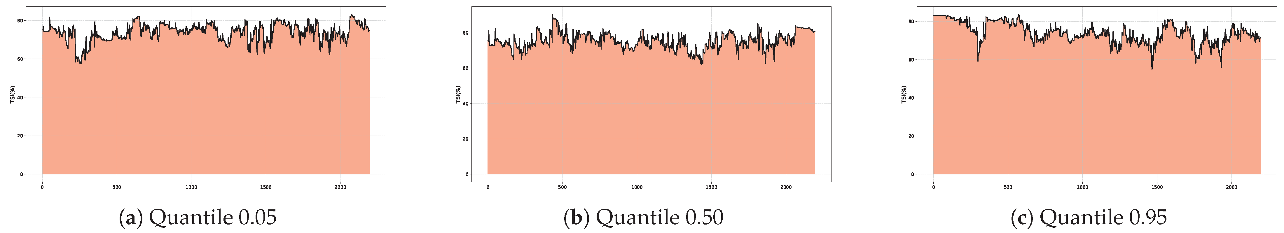
Step 1: market state classification based on the quantiles of the decomposed realized volatility components of target assets.

First, the market state is classified based on the level of a specific volatility measure, $v_{i,t}^{\left(m\right)}$, for the target asset, i. This measure may refer to realized volatility ($RV$), realized semi-variance ($RS$), the continuous component ($CV$), or the jump component ($CJ$). Using the time series $v_{i,t}^{\left(m\right)}$, the low quantile (${\tau }_L$ = 0.05) and the high quantile (${\tau }_H$ = 0.95) are computed to identify the low-volatility and high-volatility states, respectively. The market state variable, $S_t^{\left(m\right)}$, is therefore defined as follows:

$$S_t^{\left(m\right)}=\left\{\begin{array}{cc}\mathrm{Low}\text{-}\mathrm{Volatility}\hfill & \mathrm{if}{v}_{i,t}^{\left(m\right)}\le q_i^{\left(m\right)}\left({\tau }_L\right);\hfill \\ \mathrm{High}\text{-}\mathrm{Volatility}\hfill & \mathrm{if}{v}_{i,t}^{\left(m\right)}\ge q_i^{\left(m\right)}\left({\tau }_H\right);\hfill \\ \mathrm{Normal}\text{-}\mathrm{Volatility}\hfill & \mathrm{otherwise}.\hfill \end{array}\right.$$

(15)

where $q_i^{\left(m\right)}\left(\tau \right)$ is the $\tau$-th quantile of the m-th components of the realized volatility decomposition for the target asset i.

Step 2: identifying the dominant spillover source in each state.

Subsequently, the previously calculated index NPDC is employed to identify the asset, j, that exerts the largest net volatility spillover on the target asset, i, within each market state. The quantile-dependent nature of the NPDC enables a precise matching of an optimal spillover source to each market state.

• Spillover source in the low-volatility state ($j_{Low}^{*\left(m\right)}$): for the low-volatility state (defined by quantile ${\tau }_L$), the asset that generates the largest net spillover to asset i is identified as the primary spillover source.

  $$j_{Low}^{*\left(m\right)}=\underset{j\ne i}{argmax}\left({\mathrm{NPDC}}_{j\to i}^{\left(m\right)}(H,{\tau }_L)\right).$$

  (16)
• Spillover source in the high-volatility state ($j_{High}^{*\left(m\right)}$): similarly, in the high-volatility state, defined by quantile ${\tau }_H$, the asset generating the maximum net spillover is selected.

  $$j_{High}^{*\left(m\right)}=\underset{j\ne i}{argmax}\left({\mathrm{NPDC}}_{j\to i}^{\left(m\right)}(H,{\tau }_H)\right).$$

  (17)
• Spillover source in the normal-volatility state ($j_{Normal}^{*\left(m\right)}$): for the normal-volatility state, the asset with the largest net spillover at the median quantile ($\tau$ = 0.50) is selected.

  $$j_{Normal}^{*\left(m\right)}=\underset{j\ne i}{argmax}\left({\mathrm{NPDC}}_{j\to i}^{\left(m\right)}(H,0.50)\right).$$

  (18)

It is worth noting that the spillover network should be constructed using the same type of volatility data, $v^{\left(m\right)}$, as that used for the state classification. Consequently, the optimal risk source, indexed with $j^{*}$, is also dependent on the volatility type, m.

Step 3: constructing the state-dependent dynamic driving variable.

Finally, based on the identified state-dependent risk sources, a dynamic driving variable, $D_{i,t}^{\left(m\right)}$, is constructed. The value of this variable at time t is determined by the concurrent market state, $S_t^{\left(m\right)}$, and it is set to the lagged volatility ($t-1$) of the corresponding spillover source:

$$D_{i,t}^{\left(m\right)}=\left\{\begin{array}{cc}{v}_{j_{\mathrm{Low}}^{*\left(m\right)},t-1}^{\left(m\right)}\hfill & \mathrm{if}{S}_t^{\left(m\right)}=\mathrm{Low}\text{-}\mathrm{Volatility};\hfill \\ \\ v_{j_{\mathrm{High}}^{*\left(m\right)},t-1}^{\left(m\right)}\hfill & \mathrm{if}{S}_t^{\left(m\right)}=\mathrm{High}\text{-}\mathrm{Volatility};\hfill \\ \\ v_{j_{\mathrm{Normal}}^{*\left(m\right)},t-1}^{\left(m\right)}\hfill & \mathrm{if}{S}_t^{\left(m\right)}=\mathrm{Normal}\text{-}\mathrm{Volatility}.\hfill \end{array}\right.$$

(19)

The core advantage of this construction method is its ability to capture the most influential risk transmission pathways affecting the target asset’s future volatility, as identified by time-varying quantile spillovers. This renders the forecasting model both more forward-looking and economically interpretable.

2.2. Time-Varying Markov Transition Probability Model

This study adopts the Markov-Switching (MS) model proposed by Hamilton [42] as the foundational framework. In this model, the distribution of the observed variable $y_t$ depends on an unobservable discrete state variable, $S_t$, where $S_t\in \{1,2,\dots ,K\}$.

To capture the dynamic nature of risk transmission in financial markets, the approach of Bouri et al. [37] is adopted, allowing the transition probabilities between states to vary over time. Specifically, a time-varying transition probability matrix, $P_t=\left[p_{ij,t}\right]$, is constructed, where $p_{ij,t}$ denotes the probability of transitioning from state i to state j at time t. In contrast to traditional models, these probabilities are specified as functions of a state-dependent dynamic driver variable, denoted as $D_{i,t}^{\left(m\right)}$, which is constructed in the previous section. For notational convenience, $D_t$ is used to represent $D_{i,t}^{\left(m\right)}$ in the subsequent discussion. The transition probabilities are defined as follows:

$$p_{ij,t}=\mathbb{P}(S_t=j\mid S_{t-1}=i,D_t),$$

(20)

subject to the conditions $p_{ij,t}\ge 0$ and ${\sum }_{j=1}^K{p}_{ij,t}=1$.

In the empirical implementation of this paper, two latent states are considered ($K=2$): state $S_t=0$ corresponds to a low-volatility regime, while state $S_t=1$ indicates a high-volatility regime. The transition probabilities between states are specified through logistic functions to ensure they lie within the $(0,1)$ interval. Specifically, the probabilities of remaining in the same state, $p_{00,t}$ and $p_{11,t}$, are modeled as functions of the lagged dynamic driver variable $D_{t-1}$.

$$\begin{array}{cc}\hfill p_{00,t}& =\mathbb{P}(S_t=0\mid S_{t-1}=0,D_{t-1})={\displaystyle \frac{exp({\theta }_0+{\theta }_1·D_{t-1})}{1+exp({\theta }_0+{\theta }_1·D_{t-1})}},\hfill \\ \hfill p_{11,t}& =\mathbb{P}(S_t=1\mid S_{t-1}=1,D_{t-1})={\displaystyle \frac{exp({\gamma }_0+{\gamma }_1·D_{t-1})}{1+exp({\gamma }_0+{\gamma }_1·D_{t-1})}}.\hfill \end{array}$$

(21)

Here, ${\theta }_0$ and ${\gamma }_0$ are intercept terms reflecting state persistence, while ${\theta }_1$ and ${\gamma }_1$ are slope coefficients capturing the influence of the dynamic driver $D_{t-1}$ on state transitions. When all slope coefficients (e.g., ${\theta }_1$, ${\gamma }_1$) are set to zero, the model reduces to a fixed transition probability (FTP) Markov model.

Accordingly, the full $2\times 2$ time-varying transition probability matrix $P_t$ can be expressed as follows:

$$P_t=\left[\begin{array}{cc}{p}_{00,t}& 1-p_{00,t}\\ 1-p_{11,t}& p_{11,t}\end{array}\right],$$

(22)

This transition matrix, driven by external dynamic information, constitutes the core mechanism through which the proposed TVTP-MS-HAR model captures the complex dynamics of the financial market.

To incorporate time-varying regime-switching dynamics into the volatility model, this paper extends the seminal Markov-switching framework of Hamilton [42] by allowing the regime transition probabilities to vary over time as a function of observable covariates. Specifically, a covariate-dependent transition probability specification is adopted. To construct the covariate $D_{t-1}$, net spillover contributions of various assets are analyzed across different variables and quantile levels. The asset exerting the most significant spillover impact on the target market is identified, and the exogenous driver in the TVTP specification is constructed accordingly, based on the corresponding variable and quantile level.

3. Creative Research

Corsi [26] proposed the HAR model based on the heterogeneous market hypothesis, which captures both short-term and long-term volatility dynamics in financial markets. Building on this foundation, some authors [43,44] extend the HAR type model into the Markov-Switching HAR (MS-HAR) framework. This extension not only preserves the model’s ability to characterize volatility heterogeneity but also introduces regime-switching mechanisms that allow the model to capture both gradual parameter evolution and abrupt structural changes, thereby better adapting to the dynamic nature of financial markets.

3.1. Benchmark Model

Andersen and Bollerslev [8] define the realized volatility of cryptocurrency i on day t as the sum of squared intraday returns:

$${RV}_{i,t}=\sum _{l=1}^{n_t}{r}_{i,t,l}^2,$$

(23)

where $r_{i,t,l}$ denotes the l-th intraday log return of cryptocurrency i on day t, computed as follows:

$$r_{i,t,l}=(log{p}_{i,t,l}-log{p}_{i,t,l-1})\times 100.$$

(24)

Here, $p_{i,t,l}$ represents the price of asset i at the l-th intraday time point on day t.

3.1.1. MS-HAR-RV

Based on the above, the MS-HAR-RV model for cryptocurrency i is specified as follows:

$${RV}_t={\beta }_{0,S_t}+{\beta }_{1,S_t}{RV}_{t-1}+{\beta }_{2,S_t}{\overline{RV}}_{t-5}+{\beta }_{3,S_t}{\overline{RV}}_{t-22}+{ϵ}_t,$$

(25)

where $S_t\in \{0,1\}$ is a latent state variable indicating low-volatility ($S_t=0$) or high-volatility ($S_t=1$) states. The explanatory variables include daily volatility ${RV}_{t-1}$, weekly average volatility ${\overline{RV}}_{t-5}$, and monthly average volatility ${\overline{RV}}_{t-22}$. More generally, the moving average lag term is defined as follows:

$${\overline{RV}}_{t-h}={\displaystyle \frac{1}{h}}({RV}_{t-1}+\cdots +{RV}_{t-h}).$$

(26)

Following Augustyniak [45] and Cavicchioli [46], parameters are estimated via maximum likelihood. Initial parameter values are set based on model assumptions, and numerical optimization is used to maximize the log-likelihood function iteratively.

3.1.2. MS-HAR-CJ

Corsi and Reno [17] further decompose realized volatility into continuous and jump components, forming the HAR-CJ model [47]. To enhance the model’s ability to capture market dynamics, the Markov regime-switching version is defined as follows:

$$\begin{array}{cc}\hfill {RV}_t& ={\beta }_{0,S_t}+{\beta }_{1,S_t}{CV}_{t-1}+{\beta }_{2,S_t}{\overline{CV}}_{t-5}+{\beta }_{3,S_t}{\overline{CV}}_{t-22}\hfill \\ \hfill & +{\beta }_{4,S_t}{CJ}_{t-1}+{\beta }_{5,S_t}{\overline{CJ}}_{t-5}+{\beta }_{6,S_t}{\overline{CJ}}_{t-22}+{ϵ}_t,\hfill \end{array}$$

(27)

where ${CV}_{t-1}$ and ${CJ}_{t-1}$ are the lagged continuous and jump components of volatility. Their moving averages are given as follows:

$$\begin{array}{cc}\hfill {\overline{CJ}}_{t-h}& ={\displaystyle \frac{1}{h}}({CJ}_{t-1}+\cdots +{CJ}_{t-h}),\hfill \end{array}$$

(28)

$$\begin{array}{cc}\hfill {\overline{CV}}_{t-h}& ={\displaystyle \frac{1}{h}}({CV}_{t-1}+\cdots +{CV}_{t-h}).\hfill \end{array}$$

(29)

3.1.3. MS-HAR-RS

Barndorff-Nielsen et al. [48] emphasize that downside risk is more relevant for most investors. Following Patton and Sheppard [49], realized volatility is decomposed into realized semi-variances, capturing upside and downside components. The Markov-switching HAR-RS model is defined as follows:

$$\begin{array}{cc}\hfill {RV}_t& ={\beta }_{0,S_t}+{\beta }_{1,S_t}{RS}_{t-1}^{+}+{\beta }_{2,S_t}{\overline{RS}}_{t-5}^{+}+{\beta }_{3,S_t}{\overline{RS}}_{t-22}^{+}\hfill \\ \hfill & +{\beta }_{4,S_t}{RS}_{t-1}^{-}+{\beta }_{5,S_t}{\overline{RS}}_{t-5}^{-}+{\beta }_{6,S_t}{\overline{RS}}_{t-22}^{-}+{ϵ}_t.\hfill \end{array}$$

(30)

This model allows for asymmetric volatility responses to positive and negative returns across different market states. For example, the impact of negative semi-variance may intensify during financial crises but weaken during recovery periods.

3.1.4. MS-HAR-REX

Volatility in financial markets is driven by both persistent trading dynamics and sudden extreme events. To disentangle these sources, Clements and Rodriguez [50] decompose realized volatility into moderate and extreme components. The Markov-switching HAR-REX model is specified as follows:

$$\begin{array}{cc}\hfill {RV}_t& ={\beta }_{0,S_t}+{\beta }_{1,S_t}{REX}_{t-1}^{+}+{\beta }_{2,S_t}{\overline{REX}}_{t-5}^{+}+{\beta }_{3,S_t}{\overline{REX}}_{t-22}^{+}\hfill \\ \hfill & +{\beta }_{4,S_t}{REX}_{t-1}^{-}+{\beta }_{5,S_t}{\overline{REX}}_{t-5}^{-}+{\beta }_{6,S_t}{\overline{REX}}_{t-22}^{-}\hfill \\ \hfill & +{\beta }_{7,S_t}{REX}_{t-1}^m+{\beta }_{8,S_t}{\overline{REX}}_{t-5}^m+{\beta }_{9,S_t}{\overline{REX}}_{t-22}^m+{ϵ}_t.\hfill \end{array}$$

(31)

Equation (31) enables the model to capture both state-dependent and time-varying impacts of extreme positive, extreme negative, and moderate volatility, reflecting gradual shifts in microstructure and investor behaviors in cryptocurrency markets.

3.2. Innovative Model

To better capture the time-varying characteristics of the cryptocurrency market, this paper extends the traditional MS-HAR framework by allowing the state transition probabilities to be driven by external time-varying variables. This results in a Time-Varying Transition Probability Markov-Switching (TVTP-MS) model.

3.2.1. TVTP-MS-HAR-RV

Based on the theoretical foundation outlined in Section 2.1 concerning the selection of driving variables, let m denote the realized volatility metric, and let $v_{i,t}^{\left(RV\right)}$ represent the net spillover from major cryptocurrencies to Bitcoin under realized volatility. Using the quantile-specific net spillover, the key contributors to net spillovers are identified, and a time-varying driver variable, $D_{t-1}$, is constructed accordingly. (For details on net spillover contributions across quantiles and volatility types, see Appendix C 

Table A1. Net spillover contributions (%) of cryptocurrencies under different components of realized volatility.

Cryptocurrency	Quantile	$\mathit{RV}$	$\mathit{CV}$	$\mathit{CJ}$	${\mathit{RS}}^{+}$	${\mathit{RS}}^{-}$	${\mathit{REX}}^{+}$	${\mathit{REX}}^{-}$	${\mathit{REX}}^{\mathit{m}}$	$\mathit{RK}$
DASH	$\tau =0.05$	+14.77	+14.44	+14.67	+13.25	+15.99	+13.96	+12.57	+16.81	+15.99
	$\tau =0.10$	+14.62	+14.52	+14.72	+13.20	+15.68	+13.97	+12.31	+16.74	+15.68
	$\tau =0.50$	+16.74	+16.79	+17.43	+16.05	+17.53	+15.42	+13.27	+19.69	+17.53
	$\tau =0.90$	+13.91	+14.86	+16.78	+8.11	+13.56	+15.11	+14.85	+15.16	+13.56
	$\tau =0.95$	+7.56	+8.97	+8.02	+5.61	+9.26	+8.03	+10.89	+15.53	+9.26
	cyclical effect	−7.21%	−5.48%	−6.64%	−7.64%	−6.74%	−5.94%	−1.67%	−1.29%	−6.74%
ETH	$\tau =0.05$	+8.79	+9.01	+9.07	+9.12	+8.13	+10.05	+7.71	+7.14	+8.13
	$\tau =0.10$	+9.01	+9.23	+9.27	+9.39	+8.20	+10.15	+7.98	+7.03	+8.20
	$\tau =0.50$	+9.04	+9.42	+9.19	+9.75	+7.88	+10.07	+7.70	+6.35	+7.88
	$\tau =0.90$	+7.41	+7.92	+6.95	+3.60	+3.53	+5.27	+13.37	+5.24	+3.53
	$\tau =0.95$	+2.70	+5.15	+5.15	+1.61	+3.48	+2.65	+4.76	+6.77	+3.48
	cyclical effect	−6.09%	−3.86%	−3.92%	−7.51%	−4.65%	−7.41%	−2.95%	−0.37%	−4.65%
LTC	$\tau =0.05$	+14.17	+13.84	+13.88	+12.56	+15.96	+11.77	+12.85	+17.06	+15.96
	$\tau =0.10$	+14.16	+13.82	+13.88	+12.49	+16.08	+11.68	+12.58	+17.01	+16.08
	$\tau =0.50$	+15.45	+14.34	+15.52	+13.56	+15.95	+13.27	+12.20	+16.13	+15.95
	$\tau =0.90$	+10.97	+13.70	+14.04	+10.51	+7.83	+10.73	+11.78	+11.70	+7.83
	$\tau =0.95$	+11.42	+11.17	+9.53	+8.20	+8.27	+5.89	+10.17	+14.00	+8.27
	cyclical effect	−2.75%	−2.67%	−4.35%	−4.35%	−7.70%	−5.88%	−2.69%	−3.06%	−7.70%
XLM	$\tau =0.05$	+18.73	+19.23	+19.37	+18.06	+18.53	+19.23	+14.89	+19.68	+18.53
	$\tau =0.10$	+18.90	+19.46	+19.63	+17.94	+18.72	+19.32	+14.67	+19.88	+18.72
	$\tau =0.50$	+18.06	+18.99	+17.68	+17.28	+20.59	+18.77	+12.92	+21.96	+20.59
	$\tau =0.90$	+20.17	+17.24	+19.62	+22.10	+18.54	+16.62	+22.89	+18.07	+18.54
	$\tau =0.95$	+10.62	+13.77	+15.17	+31.73	+20.85	+33.83	+21.10	+12.31	+20.85
	cyclical effect	−8.11%	−5.46%	−4.19%	+13.67%	+2.31%	+14.59%	+6.21%	−7.37%	+2.31%
XRP	$\tau =0.05$	+15.99	+15.50	+15.48	+14.17	+17.41	+14.35	+13.31	+20.22	+17.41
	$\tau =0.10$	+16.12	+15.72	+15.74	+14.01	+17.55	+14.37	+13.03	+20.22	+17.55
	$\tau =0.50$	+13.01	+12.87	+12.78	+12.04	+15.76	+13.47	+11.12	+18.00	+15.76
	$\tau =0.90$	+19.34	+15.76	+17.10	+27.19	+28.29	+21.97	+17.04	+26.17	+28.29
	$\tau =0.95$	+25.29	+26.03	+35.10	+37.38	+44.89	+36.62	+37.43	+28.38	+44.89
	cyclical effect	+9.30%	+10.53%	+19.61%	+23.21%	+27.48%	+22.28%	+24.12%	+8.16%	+27.48%

Note: A positive net spillover value indicates that the cryptocurrency is a net transmitter of volatility to others, while a negative value indicates it is a net receiver.

.)

$${RV}_t={\beta }_{0,S_t\left(D_{t-1}\right)}+{\beta }_{1,S_t\left(D_{t-1}\right)}{RV}_{t-1}+{\beta }_{2,S_t\left(D_{t-1}\right)}{\overline{RV}}_{t-5}+{\beta }_{3,S_t\left(D_{t-1}\right)}{\overline{RV}}_{t-22}+{ϵ}_t.$$

(32)

3.2.2. TVTP-MS-HAR-CJ

Based on the decomposition of realized volatility discussed in Section 3.1, the continuous component ($CV$) and the jump component ($CJ$) are natural candidates for the time-varying transition probability driver. However, incorporating multiple drivers simultaneously can lead to an explosion in the number of parameters in the nonlinear component, making the numerical optimization of the likelihood function extremely challenging and potentially resulting in severe identification issues [51]. To strike a balance between model complexity and goodness of fit, model selection is guided by the Akaike Information Criterion (AIC) and the Bayesian Information Criterion (BIC).

$$\begin{array}{cc}\hfill {RV}_t& ={\beta }_{0,S_t\left(D_{t-1}\right)}+{\beta }_{1,S_t\left(D_{t-1}\right)}{CV}_{t-1}+{\beta }_{2,S_t\left(D_{t-1}\right)}{\overline{CV}}_{t-5}+{\beta }_{3,S_t\left(D_{t-1}\right)}{\overline{CV}}_{t-22}\hfill \\ \hfill & +{\beta }_{4,S_t\left(D_{t-1}\right)}{CJ}_{t-1}+{\beta }_{5,S_t\left(D_{t-1}\right)}{\overline{CJ}}_{t-5}+{\beta }_{6,S_t\left(D_{t-1}\right)}{\overline{CJ}}_{t-22}+{ϵ}_t.\hfill \end{array}$$

(33)

3.2.3. TVTP-MS-HAR-RS

A core limitation of traditional Markov-switching models (the MS-HAR-RS model in Equation (30)) is their assumption of fixed state transition probabilities, which cannot accommodate abrupt regime switching triggered by external shocks. To address this limitation, the TVTP-MS-HAR-RS model is proposed, which preserves the asymmetry-capturing ability of MS-HAR-RS while allowing the transition probabilities to vary dynamically with external information. The model is specified as follows:

$$\begin{array}{cc}\hfill {RV}_t=& {\beta }_{0,S_t\left(D_{t-1}\right)}+{\beta }_{1,S_t\left(D_{t-1}\right)}{RS}_{t-1}^{+}+{\beta }_{2,S_t\left(D_{t-1}\right)}{\overline{RS}}_{t-5}^{+}+{\beta }_{3,S_t\left(D_{t-1}\right)}{\overline{RS}}_{t-22}^{+}\hfill \\ \hfill & +{\beta }_{4,S_t\left(D_{t-1}\right)}{RS}_{t-1}^{-}+{\beta }_{5,S_t\left(D_{t-1}\right)}{\overline{RS}}_{t-5}^{-}+{\beta }_{6,S_t\left(D_{t-1}\right)}{\overline{RS}}_{t-22}^{-}+{ϵ}_t.\hfill \end{array}$$

(34)

3.2.4. TVTP-MS-HAR-REX

In extending the MS-HAR model to the TVTP-MS-HAR-REX framework, a key step is to identify the optimal external driver for state transition probabilities. Referring to the spillover network theory discussed in Section 2, three candidate drivers are constructed based on ${REX}^{+}$, ${REX}^{-}$, ${REX}^m$, and quantile-based time-varying spillovers. Each corresponding TVTP-MS-HAR-REX model is estimated and compared using AIC and BIC criteria to determine the specification with the highest predictive performance.

$$\begin{array}{cc}\hfill {RV}_t=& {\beta }_{0,S_t\left(D_{t-1}\right)}+{\beta }_{1,S_t\left(D_{t-1}\right)}{REX}_{t-1}^{+}+{\beta }_{2,S_t\left(D_{t-1}\right)}{\overline{REX}}_{t-5}^{+}+{\beta }_{3,S_t\left(D_{t-1}\right)}{\overline{REX}}_{t-22}^{+}\hfill \\ \hfill & +{\beta }_{4,S_t\left(D_{t-1}\right)}{REX}_{t-1}^{-}+{\beta }_{5,S_t\left(D_{t-1}\right)}{\overline{REX}}_{t-5}^{-}+{\beta }_{6,S_t\left(D_{t-1}\right)}{\overline{REX}}_{t-22}^{-}\hfill \\ \hfill & +{\beta }_{7,S_t\left(D_{t-1}\right)}{REX}_{t-1}^m+{\beta }_{8,S_t\left(D_{t-1}\right)}{\overline{REX}}_{t-5}^m+{\beta }_{9,S_t\left(D_{t-1}\right)}{\overline{REX}}_{t-22}^m+{ϵ}_t.\hfill \end{array}$$

(35)

4. Data and Validation

4.1. Assumptions About the Cryptocurrency Market

The dataset used in this paper is sourced from Binance, one of the world’s leading cryptocurrency exchanges. The sample includes six major cryptocurrencies: Bitcoin (BTC), Dash (DASH), Ethereum (ETH), Litecoin (LTC), Stellar (XLM), and Ripple (XRP). To mitigate microstructure noise commonly present in high-frequency data [52,53], and the empirical analysis is based on 5 min interval data. To ensure comparability across assets, the sample period is restricted to the time-frame during which complete data are available for all assets, spanning from 28 March 2019 to 30 March 2025.

Given Bitcoin’s dominant position in the cryptocurrency market [3], a core hypothesis is established: in most market states, Bitcoin functions as the primary source and net exporter of systemic volatility, whereas the other cryptocurrencies predominantly act as absorbers and net importers of this volatility.

4.2. Granger Causality Test and Multicollinearity Assessment

To further characterize the dynamic interrelationships among assets in the cryptocurrency market, this paper first conducts a preliminary examination of the predictability among six major cryptocurrencies before proceeding with the spillover analysis. Specifically, pairwise Granger causality tests are employed to identify whether there exist significant lead–lag relationships between these assets. This analysis helps uncover the relative dominance of each asset in the information transmission process and provides theoretical support and a contextual background for the construction of a volatility spillover-based dynamic network.

According to the results of the Granger causality test (lag order 2) in

Table 1. Pairwise granger causality test p-values among cryptocurrencies (lag order = 2).

Dependent Variable	BTC	DASH	ETH	LTC	XLM	XRP
BTC	1.000	0.019	0.000	0.000	0.000	0.023
DASH	0.198	1.000	0.851	0.573	0.125	0.040
ETH	0.000	0.430	1.000	0.468	0.140	0.468
LTC	0.000	0.022	0.811	1.000	0.010	0.008
XLM	0.051	0.080	0.011	0.111	1.000	0.445
XRP	0.006	0.003	0.000	0.002	0.000	1.000

, focusing on the impact of other cryptocurrencies on Bitcoin (BTC_y), DASH (p = 0.019), ETH (p = 0.000), LTC (p = 0.000), XLM (p = 0.000), and XRP (p = 0.023) all show significant predictive power for BTC, with p values all below 0.05. This suggests that the historical information of these cryptocurrencies can improve the prediction of BTC prices, indicating that BTC is strongly affected by the market dynamics driven by these assets.

To ensure the reliability of the results, given the large number of cryptocurrency variables, this paper conducts a multicollinearity analysis of the cryptocurrency market.

As shown in

Table 2. Variance inflation factor (VIF) for collinearity diagnosis.

Feature	VIF
ETH	12.708
LTC	10.823
BTC	6.959
XLM	4.354
DASH	4.193
XRP	3.330

Note: variables with VIF $\ge 10$ indicate severe multicollinearity.

, the variance inflation factor (VIF) results indicate that ETH and LTC have VIF values of 12.71 and 10.82, respectively, exceeding the commonly used threshold of 10, suggesting the presence of significant multicollinearity. However, based on the construction method of the driving variable, neither ETH nor LTC is selected under any variable at any quantile level, implying that this multicollinearity does not affect the results.

4.3. Dynamic Total Spillover Index

In reality, the transmission of information across markets and assets is often accompanied by time lags, noise, and behavioral biases among investors. Consequently, information absorption and diffusion are not instantaneous but instead unfold as a dynamic spillover process. Most existing models of information spillover rely on linear or conditional mean frameworks, which primarily focus on market co-movements under average conditions. However, in the cryptocurrency market—characterized by high volatility and frequent extreme events such as flash crashes and price surges—such homogeneous assumptions are clearly inadequate.

Given that information transfer mechanisms are far from stable in highly nonlinear environments, the intensity, direction, and even source of spillovers can vary significantly with different market mechanisms, showing clear asymmetry. Therefore, it is essential to systematically investigate the spillover network’s connectivity patterns under different market states, particularly in the distribution’s tail regions.

To investigate the dynamics and state dependence of realized volatility spillovers in the cryptocurrency market, the characteristics of the spillover network are first examined across different quantile levels within the sample period. Figure 1 presents the time series of the Time-Varying Total Spillover Index (TSI) under various quantiles $\left(\tau \right)$, illustrating how volatility spillovers evolve over time. (Other overall spillovers are shown in Appendix A Figure A1, which highlights the nonlinear heterogeneity of the spillover dynamics at different quantiles.)

To compute the parameter p in Equation (1), the method proposed by Diebold and Yilmaz [33] is followed, where the optimal lag order p is selected as 3 based on the Akaike Information Criterion (AIC) and the Bayesian Information Criterion (BIC). The forecast horizon is set to $H=10$ days, which is also consistent with Diebold and Yilmaz [33]. The quantile $\tau$ ranges from 0 to 1, and the corresponding time-varying Total Spillover Index is computed for each quantile level (see Section 2.1). The resulting spillover curves are depicted in Figure 1.

A comparison of the Total Spillover Index (TSI) across different quantiles reveals stark differences in market interdependence between low- and high-volatility states. As shown in Figure 1b, when the market is in a relatively calm state ($\tau =0.5$), the TSI fluctuates within the 60%-to-80% range. However, in the tail regions of the distribution—specifically at $\tau =0.05$ (Figure 1a) and $\tau =0.95$ (Figure 1c), the TSI systematically rises to a significantly higher level, often exceeding 65% to 85%. This finding provides strong evidence that both panic-induced sell-offs and euphoria-driven rallies sharply increase cross-market coupling, allowing investor sentiment to spread more rapidly and broadly throughout the system.

Furthermore, comparing the dynamic total spillover index estimated via the model with significant real-world economic and financial events reveals a high degree of consistency, providing strong evidence supporting the validity and real-world explanatory power of the constructed model. As illustrated clearly in Figure 1, several critical periods characterized by high spillover can be identified. For example, during the period from 2020 to 2021, starting from the global market panic triggered by the COVID-19 pandemic and followed by the substantial cryptocurrency bull market, the entire system exhibited significant volatility and interconnectedness, with the total spillover index (TSI) persistently remaining at elevated levels. Particularly noteworthy are the events in 2022, when a series of highly contagious deleveraging episodes—including the collapse of the LUNA ecosystem, the bankruptcy of Three Arrows Capital, and the liquidity crisis at the FTX exchange—triggered a systemic crisis of trust. The model accurately captures these shocks, characterized specifically by a pronounced nonlinear jump in the total spillover index. Additionally, the model reveals the market’s dynamic adjustment process following such extreme events: although tail risk indicators experience mean reversion after initially reaching peaks during the shocks, the financial system subsequently settles into a new equilibrium featuring higher interconnectedness. This finding provides new empirical evidence for understanding structural transformations in financial markets following severe shocks.

4.4. Dynamic Net Spillover Index

The previous analysis of the total spillover index reveals the overall intensity of volatility spillovers within the cryptocurrency market across different market states and periods. However, the TSI, as a macro-level indicator, cannot specify which assets primarily serve as sources of spillover effects and which assets predominantly receive these effects within the spillover network. To provide a deeper insight into the directionality and hierarchical structure of spillover transmission, as well as identify key drivers and major receivers within the system, this section further investigates the dynamic net spillover index.

The dynamic net spillover index proposed in this study accurately characterizes each asset’s dynamic role within the risk contagion network by calculating the difference between the total spillover effects that a specific asset transmits to other assets and the total spillover effects it receives from others at any given point in time. Analyzing this index enables the identification of cryptocurrencies that act as core drivers of systemic spillover under various market conditions (defined by quantiles $\left(\tau \right)$) and further allows observation of whether these assets change their market roles over time.

To investigate the transmission mechanism of the cryptocurrency market under downside tail-risk conditions, this section analyzes the dynamic net spillover index at the quantile $(\tau =0.05)$, as illustrated by Figure 2. During periods of market distress, most assets act as net spillover transmitters (dominated by green regions), reflecting systemic risk-averse sentiment. Nevertheless, assets exhibit notable heterogeneity and dynamic role transitions. Specifically, Bitcoin (Figure 2a) primarily functions as a net spillover receiver (dominated by red regions) but experiences a significant role reversal during systemic crises, such as the market crash in 2022, becoming the principal net spillover transmitter. Ethereum (Figure 2b) and Ripple (Figure 2c) consistently maintain net receiver positions, serving as stable spillover buffers, while Dash (Figure 2d) and Stellar (Figure 2e) demonstrate highly unstable, impulsive spillover behaviours, frequently switching between transmitter and receiver roles. These findings underscore the importance of identifying state-dependent driving variables capable of predicting Bitcoin’s spillover role transitions, thereby laying a solid empirical foundation for subsequent modeling efforts.

As shown in Figure 3, the spillover transmission pattern at the median quantile ($\tau =0.5$) differs significantly from the downside tail-risk state ($\tau =0.05$). Under neutral market conditions, assets exhibit more frequent role transitions and generally lower magnitudes of net spillovers, indicating milder volatility spillover and a lack of persistent dominant forces. In this state, Bitcoin (Figure 3a) displays subtle role changes: although still predominantly a net spillover receiver during 2022–2023, its net spillover fluctuates around zero and occasionally turns positive, weakening its central position. Similarly, Ethereum (Figure 3c) remains a net receiver, but the intensity of its spillover absorption is clearly reduced. Notably, Dash (Figure 3b) and Ripple (Figure 3f) emerge as prominent net spillover transmitters in neutral market conditions, particularly between 2020 and 2022, indicating their volatility serves as an important source of information transmission and disturbance to the broader system. Overall, the spillover network in normal market states appears more dispersed and multipolar compared to extreme market conditions, further supporting the necessity and effectiveness of employing a quantile-based approach to capture state-dependent spillover dynamics.

Under extreme upward market conditions ($\tau =0.95$), the spillover network exhibits structural features distinctly different from those observed under neutral market conditions ($\tau =0.5$). Most notably, almost all cryptocurrencies become net spillover transmitters (dominated by green regions), sharply contrasting with the widespread risk absorption observed under extreme downside market states ($\tau =0.05$). In this scenario, Bitcoin (Figure 4a) and Ethereum (Figure 4c) significantly enhance their market leadership roles, their stable and persistent positive spillovers constituting the core driving force behind the upward market interconnectedness. Ripple (Figure 4f) also emerges as a powerful and sustained net transmitter, with its influence at times comparable to that of Ethereum, potentially due to its strong community consensus. By comparison, other mainstream cryptocurrencies (such as Dash, Litecoin, and Stellar) exhibit more impulsive and unstable net spillover patterns.

4.5. Heatmap of Dynamic Net Spillover Indices

The previous analyses of total and net spillovers have examined the dynamic evolution and hierarchical structure of the cryptocurrency spillover network from the perspectives of overall intensity and individual market roles. To further investigate the transmission paths of dominant net spillover sources and the primary exposure channels of net spillover receivers, this section employs heatmap visualizations of the spillover matrices. This analytical framework provides more detailed empirical evidence on the internal topological structure of the cryptocurrency market spillover network.

Figure 5 illustrates that the cryptocurrency spillover network exhibits significant state-dependent and asymmetric characteristics. These results indicate that the risk transmission structure fundamentally differs between market regimes, such as tranquil versus turbulent periods. The analyses for the remaining quantiles are presented in Appendix B Figure A2.

4.6. Quantifying Spillover Contributions

While the preceding heatmap analysis visually reveals the complex, directed structure of the spillover network, the ultimate goal of selecting a dynamic driving variable for our Bitcoin volatility model requires a quantitative comparison and ranking of these spillover relationships. To this end, this section further investigates the pairwise spillover contributions to Bitcoin. It systematically calculates and presents the average directional spillover strength from each candidate cryptocurrency to Bitcoin across different quantiles, aiming to provide a robust empirical basis for our variable selection.

Figure 6 presents the net spillover effects from major cryptocurrencies to Bitcoin under various market conditions, based on multiple realized volatility measures and their decomposed components. The analysis reveals significant asymmetry in cryptocurrency volatility spillovers, primarily driven by extreme market optimism, rather than pessimism. Across all volatility measures, the net spillover curves rise sharply during extreme market upturns (right tail, $\tau \ge$ 0.90), while responses to extreme downturns (left tail) remain relatively moderate.

The further decomposition of volatility indicates that this asymmetry mainly arises from the jump component ($JV$, Figure 6d) and realized positive semi-variance (${RS}^{+}$, Figure 6e). In contrast, the net spillover based on realized negative semi-variance (${RS}^{-}$, Figure 6f) remains relatively flat. Additionally, the analysis identifies key “risk transmitter cores” within the network, exemplified by assets such as XRP or XLM (indicated by the light blue curves), which consistently act as dominant net spillover transmitters across all market conditions, especially during extreme events.

4.7. Synthesis of Analytical Findings

In Section 4.1, this paper proposes a hypothesis regarding the cryptocurrency market and demonstrates its validity through analyses of the dynamic total spillover, dynamic net spillover, and heatmap visualizations.

5. Empirical Results

5.1. Descriptive Statistics of Sample Data

Table 3. Descriptive statistics of realized volatility and its decomposed components.

Variable	Mean	Std. Dev.	Skewness	Kurtosis	Max	Min	ADF	LB(10)
$RV$	13.569	35.885	19.842	547.789	158.821	0.083	−12.575 ***	831.391 ***
$JV$	1.385	4.208	8.884	111.953	76.563	0.000	−15.772 ***	73.426 ***
$CV$	12.090	34.194	20.639	569.046	104.436	0.067	−13.773 ***	785.166 ***
$R{S}^{+}$	6.788	20.253	25.313	851.994	746.307	0.044	−12.814 ***	512.327 ***
$R{S}^{-}$	6.780	16.788	14.971	304.790	412.514	0.039	−13.268 ***	981.463 ***
$RE{X}^{-}$	3.949	10.760	15.420	321.669	267.442	0.019	−16.321 ***	500.178 ***
$RE{X}^{+}$	3.997	14.197	27.010	927.454	531.921	0.027	−13.720 ***	287.222 ***
$RE{X}^m$	5.531	13.476	20.423	617.690	460.552	0.037	−11.730 ***	1137.543 ***

Notes: This table presents descriptive statistics. RV is realized volatility, JV is the jump component, CV is the continuous component, RS⁺ and RS⁻ are positive/negative semi-variance, and REX⁺, REX⁻, and REX^m are positive, negative, and moderate volatility. ADF is the augmented Dickey–Fuller test statistic. LB(10) is the Ljung–Box Q-statistic for serial correlation up to 10 lags. *** Significance at the 0.01 level.

reports the descriptive statistics for realized volatility ($RV$) and its decomposed components. The statistics reveal that the distribution of $RV$ is significantly right-skewed and leptokurtic, suggesting the presence of extreme values and a higher-than-normal probability of their occurrence. Furthermore, the augmented Dickey–Fuller (ADF) test statistics for all variables are significantly negative at the 0.01 level, indicating that all series are stationary.

Figure 7a plots the time series of Bitcoin’s realized volatility. A distinct feature is the dramatic spike in early 2020, which coincides with the global outbreak of the COVID-19 pandemic and the subsequent financial market turmoil. The extreme volatility during this period likely reflects the unprecedented macroeconomic uncertainty driven by the pandemic, as well as the heightened interconnectedness between the cryptocurrency and traditional financial markets.

The full dataset is partitioned into a training set (in-sample) and a testing set (out-of-sample). The training set, comprising the first 80% of the observations, spans from 19 April 2019 to 20 January 2024, and is used for model estimation. The remaining 20% of the data forms the testing set, covering the period from 21 January 2024 to 30 March 2025, which is reserved for out-of-sample performance evaluation. The parameter estimation results from the training set are reported in

Table 4. Parameter estimation results for MS-HAR-type models.

	MS-HAR-RV		MS-HAR-CJ		MS-HAR-RS		MS-HAR-REX
State	${\mathit{S}}_{\mathbf{0}}$	${\mathit{S}}_{\mathbf{1}}$	${\mathit{S}}_{\mathbf{0}}$	${\mathit{S}}_{\mathbf{1}}$	${\mathit{S}}_{\mathbf{0}}$	${\mathit{S}}_{\mathbf{1}}$	${\mathit{S}}_{\mathbf{0}}$	${\mathit{S}}_{\mathbf{1}}$
${\beta }_0$	$2.503$***	$46.607$***	$2.691$***	$49.606$***	$2.541$***	$31.965$***	$2.487$***	$29.494$***
	$\left(0.147\right)$	$\left(9.107\right)$	$\left(0.169\right)$	$\left(10.462\right)$	$\left(0.150\right)$	$\left(7.216\right)$	$\left(0.140\right)$	$\left(6.995\right)$
${\beta }_1$	$0.237$***	$0.254$***	$-0.057$*	$-0.327$	$0.333$***	$-1.507$***	$-0.002$	$3.453$***
	$\left(0.010\right)$	$\left(0.079\right)$	$\left(0.032\right)$	$\left(0.998\right)$	$\left(0.028\right)$	$\left(0.218\right)$	$\left(0.023\right)$	$\left(0.368\right)$
${\beta }_2$	$0.171$***	$0.150$	$0.024$	$2.348$	$0.340$***	$-1.138$	$-0.022$	$2.131$
	$\left(0.010\right)$	$\left(0.164\right)$	$\left(0.065\right)$	$\left(3.254\right)$	$\left(0.052\right)$	$\left(1.100\right)$	$\left(0.053\right)$	$\left(1.435\right)$
${\beta }_3$	$0.112$***	$-0.166$	$0.006$	$-4.057$	$0.040$*	$-2.398$	$-0.017$	$-1.690$
	$\left(0.009\right)$	$\left(0.299\right)$	$\left(0.108\right)$	$\left(5.379\right)$	$\left(0.024\right)$	$\left(3.633\right)$	$\left(0.101\right)$	$\left(3.732\right)$
${\beta }_4$			$0.272$***	$0.296$***	$0.002$	$2.532$***	$0.008$	$-1.039$*
			$\left(0.012\right)$	$\left(0.081\right)$	$\left(0.056\right)$	$\left(0.310\right)$	$\left(0.029\right)$	$\left(0.531\right)$
${\beta }_5$			$0.171$***	$0.086$	$0.079$	$1.641$	$0.099$	$-0.648$
			$\left(0.011\right)$	$\left(0.186\right)$	$\left(0.093\right)$	$\left(1.312\right)$	$\left(0.065\right)$	$\left(1.366\right)$
${\beta }_6$			$0.131$***	$-0.080$	$0.197$*	$2.194$	$-0.256$ **	$0.140$
			$\left(0.011\right)$	$\left(0.387\right)$	$\left(0.102\right)$	$\left(3.981\right)$	$\left(0.095\right)$	$\left(3.089\right)$
${\beta }_7$							$0.572$***	$0.021$
							$\left(0.040\right)$	$\left(0.616\right)$
${\beta }_8$							$0.338$***	$-0.542$
							$\left(0.061\right)$	$\left(1.240\right)$
${\beta }_9$							$0.459$***	$0.760$
							$\left(0.073\right)$	$\left(2.184\right)$
$p_{00}$	$0.927$***		$0.925$***		$0.918$***		$0.911$***
	$\left(0.007\right)$		$\left(0.007\right)$		$\left(0.007\right)$		$\left(0.007\right)$
$p_{11}$		$0.500$***		$0.493$***		$0.486$***		$0.451$***
		$\left(0.034\right)$		$\left(0.033\right)$		$\left(0.032\right)$		$\left(0.032\right)$
${\sigma }_{S_0}^2$	$4.082$***		$94.541$***		$3.935$***		$92.969$***
	$\left(0.074\right)$		$\left(4.495\right)$		$\left(0.072\right)$		$\left(4.390\right)$
${\sigma }_{S_1}^2$		$3.912$***		$72.235$***		$3.639$***		$67.712$***
		$\left(0.071\right)$		$\left(3.308\right)$		$\left(0.067\right)$		$\left(3.080\right)$
Log-Likelihood	$-6040.723$		$-6003.270$		$-5988.631$		$-5897.603$
AIC	12,105.446		12,042.539		12,013.263		11,843.206
BIC	12,170.972		12,140.828		12,111.552		11,974.246

Note: *, **, and *** indicate significance at the 0.1, 0.05, and 0.01 levels, respectively. Standard errors are reported in parentheses. State $S_0$ corresponds to the low-volatility state (State 0), and $S_1$ corresponds to the high-volatility state (State 1).

.

To investigate the economic forces driving these regime shifts, the analysis is extended to a Time-Varying Transition Probability (TVTP-MS-HAR) model. This specification allows the transition probabilities between states to vary dynamically with external driving variables. As shown in

Table 5. Parameter estimation results for TVTP-MS-HAR-type models.

	TVTP-MS-HAR-RV		TVTP-MS-HAR-CJ		TVTP-MS-HAR-RS		TVTP-MS-HAR-REX
State	${\mathit{S}}_{\mathbf{0}}$	${\mathit{S}}_{\mathbf{1}}$	${\mathit{S}}_{\mathbf{0}}$	${\mathit{S}}_{\mathbf{1}}$	${\mathit{S}}_{\mathbf{0}}$	${\mathit{S}}_{\mathbf{1}}$	${\mathit{S}}_{\mathbf{0}}$	${\mathit{S}}_{\mathbf{1}}$
${\beta }_0$	$2.406$***	$45.114$***	$2.270$***	$10.891$	$2.348$***	$23.252$***	$2.387$***	$8.721$***
	$\left(0.201\right)$	$\left(8.903\right)$	$\left(0.197\right)$	$\left(9.476\right)$	$\left(0.185\right)$	$\left(7.283\right)$	$\left(0.160\right)$	$\left(7.024\right)$
${\beta }_1$	$0.251$***	$0.252$***	$-0.004$	$-0.391$	$0.377$***	$-1.323$	$0.550$***	$-0.499$
	$\left(0.014\right)$	$\left(0.076\right)$	$\left(0.036\right)$	$\left(0.987\right)$	$\left(0.037\right)$	$\left(0.945\right)$	$\left(0.051\right)$	$\left(0.597\right)$
${\beta }_2$	$0.165$***	$0.148$	$-0.298$***	$2.549$	$0.307$***	$-0.860$	$0.373$***	$-0.613$
	$\left(0.014\right)$	$\left(0.160\right)$	$\left(0.073\right)$	$\left(3.377\right)$	$\left(0.059\right)$	$\left(1.166\right)$	$\left(0.055\right)$	$\left(1.127\right)$
${\beta }_3$	$0.114$***	$-0.156$	$0.172$	$2.187$	$0.060$	$-7.353$*	$0.025$	$2.123$
	$\left(0.019\right)$	$\left(0.290\right)$	$\left(0.392\right)$	$\left(17.061\right)$	$\left(0.101\right)$	$\left(3.908\right)$	$\left(0.034\right)$	$\left(1.927\right)$
${\beta }_4$			$0.238$***	$0.334$***	$0.086$***	$2.251$***	$0.026$	$1.236$
			$\left(0.022\right)$	$\left(0.080\right)$	$\left(0.029\right)$	$\left(0.344\right)$	$\left(0.029\right)$	$\left(0.217\right)$
${\beta }_5$			$0.131$***	$0.131$	$0.023$	$-2.397$	$-0.047$	$1.240$
			$\left(0.038\right)$	$\left(0.145\right)$	$\left(0.064\right)$	$\left(1.399\right)$	$\left(0.059\right)$	$\left(1.317\right)$
${\beta }_6$			$0.220$***	$2.200$	$0.192$*	$7.798$*	$-0.003$	$-2.133$
			$\left(0.172\right)$	$\left(17.186\right)$	$\left(0.108\right)$	$\left(4.263\right)$	$\left(0.026\right)$	$\left(3.022\right)$
${\beta }_7$							$0.057$**	$1.347$***
							$\left(0.029\right)$	$\left(0.322\right)$
${\beta }_8$							$-0.107$	$3.002$**
							$\left(0.066\right)$	$\left(1.434\right)$
${\beta }_9$							$-0.011$	$0.294$
							$\left(0.109\right)$	$\left(3.609\right)$
${\theta }_0$	$2.584$***		$2.642$***		$2.617$***		$2.498$***
	$\left(0.131\right)$		$\left(0.123\right)$		$\left(0.150\right)$		$\left(0.150\right)$
${\theta }_1$		$-0.604$**		$-0.498$**		$-0.574$**		$-0.498$***
		$\left(0.254\right)$		$\left(0.255\right)$		$\left(0.227\right)$		$\left(0.182\right)$
${\gamma }_0$	$-0.003$*		$-0.002$		$-0.019$***		$-0.049$***
	$\left(0.002\right)$		$\left(0.001\right)$		$\left(0.006\right)$		$\left(0.010\right)$
${\gamma }_1$		$0.007$**		$0.008$**		$0.010$**		$0.060$***
		$\left(0.003\right)$		$\left(0.003\right)$		$\left(0.004\right)$		$\left(0.018\right)$
$p_{00}$	$0.922$***		$0.915$***		$0.909$***		$0.949$***
	$\left(0.089\right)$		$\left(0.001\right)$		$\left(0.009\right)$		$\left(0.001\right)$
$p_{11}$		$0.407$***		$0.397$***		$0.399$***		$0.384$***
		$\left(0.003\right)$		$\left(0.043\right)$		$\left(0.046\right)$		$\left(0.038\right)$
${\sigma }_{S_0}^2$	$1.923$***		$1.982$***		$1.833$***		$1.672$***
	$\left(0.091\right)$		$\left(0.073\right)$		$\left(0.089\right)$		$\left(0.078\right)$
${\sigma }_{S_1}^2$		$20.548$***		$20.848$***		$18.473$***		$17.665$***
		$\left(0.462\right)$		$\left(0.481\right)$		$\left(0.421\right)$		$\left(0.429\right)$
Log-likelihood	$-6037.541$		$-6003.005$		$-5964.771$		$-5882.366$
AIC	12,095.082		12,036.01		11,959.542		11,804.732
BIC	12,161.608		12,117.856		12,066.770		11,943.069

Note: *, **, and *** indicate significance at the 0.1, 0.05, and 0.01 levels, respectively. Standard errors are reported in parentheses. All estimates are rounded to three decimal places.

, the TVTP-MS-HAR models also identify distinct low- and high-volatility regimes. More importantly, the estimated coefficients for the driving variables ($\theta$ and $\gamma$) are highly significant at the 0.01 level, providing strong evidence for their effectiveness in explaining the dynamics of volatility state transitions.

Compared to fixed transition probability models, the key contribution of the time-varying transition probability (TVTP) model lies in its ability to reveal the dynamic characteristics of transition probabilities. Coefficient estimates of the TVTP models indicate that the driving variables in the TVTP-MS-HAR-CJ, TVTP-MS-HAR-RS, and TVTP-MS-HAR-REX models significantly affect state transition probabilities. A notable finding is that, under the HAR, MS-HAR, and TVTP-MS-HAR modeling frameworks, the X-RV model consistently demonstrates superior predictive performance, significantly outperforming other competing models.

Although volatility–component–decomposition-based models such as HAR-CJ and HAR-RS have exhibited distinct advantages in forecasting traditional financial markets [54], their predictive efficacy diminishes considerably in the Bitcoin market. This discrepancy may originate from the unique complex dynamic characteristics inherent to Bitcoin markets. As highlighted by Ang and Bekaert [51], Bitcoin markets exhibit chaotic dynamics, multifractality, and pronounced regime-switching behaviors. In such highly nonlinear market environments, decomposing realized volatility into continuous and jump components (or signed semi-variance) may introduce substantial estimation errors, as these decomposed components display notable instability in their autoregressive patterns across different market regimes. Therefore, the simpler and more robust HAR-RV model, by modeling aggregated total volatility directly and thus avoiding potential specification biases due to unstable microstructure decomposition, exhibits stronger competitiveness in out-of-sample forecasting.

5.2. Out-of-Sample Forecasting Design and Evaluation

To rigorously evaluate the out-of-sample forecasting performance of the TVTP-MS-HAR models, this study employs a rolling window forecasting scheme. The forecasting procedure is implemented as follows:

(1)

The total sample is partitioned into an initial estimation window and a subsequent out-of-sample prediction period. Following the data partitioning described in Section 5.1, the initial estimation window is fixed at 1800 observations (from 19 April 2019 to 4 June 2024). The out-of-sample period consists of the final 300 observations (from 5 June 2024 to 30 March 2025).

(2)

The TVTP-MS-HAR models are first estimated using the initial 1800 observations (from $t=1,\dots ,H=1800$). The estimated parameters are then used to generate a one-step-ahead forecast of volatility, ${\widehat{\sigma }}_{H+1}^2$. This process is repeated to obtain five-day-ahead and twenty-two-day-ahead forecasts.

(3)

The estimation window is then rolled forward by one observation, maintaining a fixed window size of 1800. The models are re-estimated with each new window to produce the next forecast (${\widehat{\sigma }}_{H+2}^2$, and so on). This re-estimation at each step ensures that the forecasts adapt to the most recent information available.

To evaluate the forecast accuracy, this study adopts two distinct loss functions, a practice recommended by scholars such as Hyndman and Koehler [55], Aït-Sahalia and Mancini [56], and Hansen [57]. Let ${\widehat{\sigma }}_m^2$ be the out-of-sample forecast for period m, and $R{V}_m$ be the corresponding realized volatility. H denotes the length of the estimation window, and M is the number of forecasts. The loss functions are defined as follows:

$$MSE={\displaystyle \frac{1}{M}}\sum _{m=H+1}^{H+M}{(R{V}_m-{\widehat{\sigma }}_m^2)}^2,$$

(36)

$$QLIKE={\displaystyle \frac{1}{M}}\sum _{m=H+1}^{H+M}\left(ln\left({\widehat{\sigma }}_m^2\right)+{\displaystyle \frac{R{V}_m}{{\widehat{\sigma }}_m^2}}\right),$$

(37)

where $MSE$ denotes the mean squared error and $QLIKE$ represents the quasi-likelihood loss function.

The reliance on a single loss function for model comparison can be restrictive, as the resulting ranking may not be robust to the choice of evaluation metric or the underlying data-generating process. Outliers, in particular, can disproportionately influence the value of certain loss functions (like $MSE$), potentially leading to erroneous conclusions about a model’s forecasting superiority. By using both $MSE$, which penalizes large errors quadratically, and $QLIKE$, which is more robust for variance forecasting, we aim to provide a more comprehensive and reliable assessment of the models.

Based on this, numerous scholars have proposed various approaches to evaluate the out-of-sample forecasting accuracy of models, such as those developed by White [58] and Diebold and Mariano [59]. However, currently, the most widely used method in practice is the model confidence set (MCS) approach proposed by Hansen and Lunde [60]. (For the specific MCS inspection process, see Appendix D.)

The MCS test is utilized to select the optimal forecasting models at a given confidence level. The test statistics, $T_R$ and $T_{\max }$, and their corresponding p-values are obtained through 5000 bootstrap iterations. In evaluating forecasting models, the MCS test is typically performed using the loss functions ${QLIKE}_{\alpha }$ and ${MSE}_{\alpha }$. Three confidence levels, namely $\alpha \in \{0.01,0.1,0.25\}$, are selected, resulting in three corresponding model confidence sets denoted as $M_{0.99}^{*}$, $M_{0.90}^{*}$, and $M_{0.75}^{*}$. A higher significance level (a smaller $\alpha$) corresponds to fewer models included in the MCS. Specifically, if a forecasting model’s p-value falls below 0.01, it indicates poor out-of-sample predictive performance at this significance level; conversely, a p-value above 0.01 implies that the model survives within the confidence set $M_{0.99}^{*}$.

To better illustrate the forecasting accuracy of the models, some fundamental benchmark models ([60,61]) are compared with the time-varying Markov-switching models. Figure 8 shows the comparative results of one-step-ahead forecasts from various models. The black solid line represents the actual realized volatility, while the dashed lines in 18 different colors depict forecasts from different models. It can be observed that the black realized volatility line exhibits several abnormal peaks, and notably, the yellow dashed line representing the TVTP-MS model closely fits these peaks.

To further evaluate the out-of-sample forecasting performance of each model, the MCS approach is applied under both $QLIKE$ and $MSE$ loss functions to test the forecasting results of GARCH-type, HAR-type, MS-HAR-type, and TVTP-MS-HAR-type models. The significance levels $\alpha$ are set to 0.01, 0.10, and 0.25, respectively, with the results summarized in

Table 6. MCS test results for one-step-ahead out-of-sample forecasting.

Model	${\mathit{QLIKE}}_{{\mathit{\alpha }}_1}$		${\mathit{MSE}}_{{\mathit{\alpha }}_1}$		${\mathit{QLIKE}}_{{\mathit{\alpha }}_2}$		${\mathit{MSE}}_{{\mathit{\alpha }}_2}$		${\mathit{QLIKE}}_{{\mathit{\alpha }}_3}$		${\mathit{MSE}}_{{\mathit{\alpha }}_3}$
	${\mathit{T}}_{\mathit{max}}$	${\mathit{T}}_{\mathit{R}}$	${\mathit{T}}_{\mathit{max}}$	${\mathit{T}}_{\mathit{R}}$	${\mathit{T}}_{\mathit{max}}$	${\mathit{T}}_{\mathit{R}}$	${\mathit{T}}_{\mathit{max}}$	${\mathit{T}}_{\mathit{R}}$	${\mathit{T}}_{\mathit{max}}$	${\mathit{T}}_{\mathit{R}}$	${\mathit{T}}_{\mathit{max}}$	${\mathit{T}}_{\mathit{R}}$
GARCH-type models
GARCH	$0.000$	$0.000$	$1.000$	$0.038$	$0.000$	$0.000$	$0.222$	$0.030$	$0.000$	$0.000$	$0.000$	$0.000$
EGARCH	$0.000$	$0.000$	$1.000$	$0.056$	$0.000$	$0.000$	$0.292$	$0.050$	$0.000$	$0.000$	$0.000$	$0.000$
GARCH-M	$0.000$	$0.000$	$1.000$	$0.058$	$0.000$	$0.000$	$0.181$	$0.058$	$0.000$	$0.000$	$0.000$	$0.000$
GJR-GARCH	$0.000$	$0.000$	$1.000$	$0.044$	$0.000$	$0.000$	$0.236$	$0.036$	$0.000$	$0.000$	$0.000$	$0.000$
FIGARCH	$0.000$	$0.000$	$1.000$	$0.000$	$0.000$	$0.000$	$0.120$	$0.000$	$0.000$	$0.000$	$0.000$	$0.000$
APARCH	$0.000$	$0.000$	$1.000$	$0.044$	$0.000$	$0.000$	$0.268$	$0.036$	$0.000$	$0.000$	$0.000$	$0.000$
HAR-type models
HAR-RV	$0.488$	$0.008$	$1.000$	$0.148$	$0.503$	$0.011$	$1.000$	$0.124$	$0.444$	$0.011$	$0.732$	$0.064$
HAR-CJ	$0.163$	$0.004$	$1.000$	$0.124$	$0.162$	$0.005$	$1.000$	$0.109$	$0.921$	$0.011$	$0.268$	$0.054$
HAR-RS	$0.979$	$0.801$	$1.000$	$0.056$	$0.978$	$0.779$	$1.000$	$0.050$	$0.988$	$0.782$	$0.000$	$0.000$
HAR-REX	$1.000$	$0.463$	$1.000$	$0.034$	$1.000$	$0.431$	$1.000$	$0.027$	$1.000$	$0.438$	$0.000$	$0.000$
MS-HAR-type models
MS-HAR-RV	$1.000$	$0.463$	$0.031$	$0.079$	$1.000$	$0.431$	$0.000$	$0.000$	$0.981$	$0.416$	$0.000$	$0.000$
MS-HAR-CJ	$1.000$	$0.463$	$0.048$	$0.109$	$1.000$	$0.431$	$0.000$	$0.000$	$0.958$	$0.416$	$0.000$	$0.000$
MS-HAR-RS	$0.999$	$0.349$	$0.065$	$0.109$	$1.000$	$0.338$	$0.000$	$0.000$	$0.958$	$0.338$	$0.000$	$0.000$
MS-HAR-REX	$1.000$	$0.463$	$0.064$	$0.109$	$1.000$	$0.431$	$0.000$	$0.000$	$1.000$	$0.438$	$0.000$	$0.000$
TVTP-MS-HAR-type models
TVTP-MS-HAR-RV	$1.000$	$\mathbf{1.000}$	$\mathbf{1.000}$	$\mathbf{1.000}$	$1.000$	$\mathbf{1.000}$	$\mathbf{1.000}$	$\mathbf{1.000}$	$1.000$	$\mathbf{1.000}$	$\mathbf{1.000}$	$\mathbf{1.000}$
TVTP-MS-HAR-CJ	$1.000$	$1.000$	$1.000$	$1.000$	$1.000$	$1.000$	$1.000$	$1.000$	$1.000$	$1.000$	$1.000$	$1.000$
TVTP-MS-HAR-RS	$1.000$	$1.000$	$1.000$	$1.000$	$1.000$	$1.000$	$1.000$	$1.000$	$1.000$	$1.000$	$1.000$	$1.000$
TVTP-MS-HAR-REX	$\mathbf{1.000}$	$1.000$	$1.000$	$1.000$	$\mathbf{1.000}$	$1.000$	$1.000$	$0.908$	$\mathbf{1.000}$	$1.000$	$0.971$	$0.908$

Note: ${\alpha }_1$, ${\alpha }_2$, and ${\alpha }_3$ represent the significance levels of the MCS test at 0.01, 0.1, and 0.25, respectively. The p-value indicates the model’s forecasting accuracy, with higher p-values indicating better accuracy. The p-value of the top-ranked model is shown in bold, indicating the best forecasting performance under the corresponding loss function and test statistic.

. The empirical results clearly highlight differences in forecasting accuracy across model families. First, all GARCH-type models are excluded at the significance level ${\alpha }_3$, indicating significantly inferior predictive performance compared to other models. Second, standard HAR-type and fixed-regime MS-HAR-type models exhibit moderate competitiveness, remaining in the confidence sets in most cases, but never achieving optimal rankings. In stark contrast, the TVTP-MS-HAR-type model consistently demonstrates superior predictive performance. Specifically, TVTP-MS-HAR-RV, TVTP-MS-HAR-CJ, and TVTP-MS-HAR-RS consistently rank among the best-performing models under both $QLIKE$ and $MSE$ loss functions, with their p-values typically equal to 1.000 in most tests, often attaining the top ranking (highlighted in bold). These findings underscore that incorporating a time-varying Markov regime-switching mechanism into HAR models effectively captures the dynamic features of volatility, thereby substantially outperforming traditional GARCH models, standard HAR models, and fixed-transition-probability MS-HAR models in terms of out-of-sample forecasting accuracy.

To further evaluate models’ medium- to long-term forecasting performance,

Table 7. MCS test results for five-step-ahead out-of-sample forecasting.

Model	${\mathit{QLIKE}}_{{\mathit{\alpha }}_1}$		${\mathit{MSE}}_{{\mathit{\alpha }}_1}$		${\mathit{QLIKE}}_{{\mathit{\alpha }}_2}$		${\mathit{MSE}}_{{\mathit{\alpha }}_2}$		${\mathit{QLIKE}}_{{\mathit{\alpha }}_3}$		${\mathit{MSE}}_{{\mathit{\alpha }}_3}$
	${\mathit{T}}_{\mathit{max}}$	${\mathit{T}}_{\mathit{R}}$	${\mathit{T}}_{\mathit{max}}$	${\mathit{T}}_{\mathit{R}}$	${\mathit{T}}_{\mathit{max}}$	${\mathit{T}}_{\mathit{R}}$	${\mathit{T}}_{\mathit{max}}$	${\mathit{T}}_{\mathit{R}}$	${\mathit{T}}_{\mathit{max}}$	${\mathit{T}}_{\mathit{R}}$	${\mathit{T}}_{\mathit{max}}$	${\mathit{T}}_{\mathit{R}}$
GARCH-type models
GARCH	$0.000$	$0.000$	$0.901$	$0.048$	$0.000$	$0.000$	$0.179$	$0.045$	$0.000$	$0.000$	$0.000$	$0.000$
EGARCH	$0.000$	$0.000$	$0.900$	$0.102$	$0.000$	$0.000$	$0.314$	$0.084$	$0.000$	$0.000$	$0.000$	$0.000$
GARCH-M	$0.000$	$0.000$	$0.900$	$0.058$	$0.000$	$0.000$	$0.181$	$0.058$	$0.000$	$0.000$	$0.000$	$0.000$
GJR-GARCH	$0.000$	$0.000$	$1.000$	$0.000$	$0.000$	$0.000$	$0.210$	$0.001$	$0.000$	$0.000$	$0.000$	$0.000$
FIGARCH	$0.000$	$0.000$	$1.000$	$0.000$	$0.000$	$0.000$	$0.000$	$0.000$	$0.000$	$0.000$	$0.000$	$0.000$
APARCH	$0.000$	$0.000$	$1.000$	$0.063$	$0.000$	$0.000$	$0.279$	$0.058$	$0.000$	$0.000$	$0.000$	$0.000$
HAR-type models
HAR-RV	$0.000$	$0.000$	$0.000$	$0.000$	$0.000$	$0.000$	$0.000$	$0.000$	$0.000$	$0.000$	$0.000$	$0.000$
HAR-CJ	$0.561$	$0.029$	$1.000$	$0.046$	$0.574$	$0.031$	$0.181$	$0.035$	$0.545$	$0.030$	$0.000$	$0.000$
HAR-RS	$1.000$	$0.794$	$1.000$	$0.191$	$1.000$	$0.799$	$0.893$	$0.171$	$1.000$	$0.790$	$0.000$	$0.000$
HAR-REX	$1.000$	$0.836$	$1.000$	$0.102$	$1.000$	$0.837$	$0.253$	$0.084$	$1.000$	$0.836$	$0.000$	$0.000$
MS-HAR-type models
MS-HAR-RV	$0.280$	$0.020$	$0.014$	$0.043$	$0.290$	$0.019$	$0.000$	$0.000$	$0.275$	$0.017$	$0.000$	$0.000$
MS-HAR-CJ	$0.445$	$0.074$	$0.012$	$0.043$	$0.448$	$0.073$	$0.000$	$0.000$	$0.445$	$0.072$	$0.000$	$0.000$
MS-HAR-RS	$0.286$	$0.010$	$0.048$	$0.044$	$0.301$	$0.008$	$0.000$	$0.000$	$0.288$	$0.010$	$0.000$	$0.000$
MS-HAR-REX	$0.709$	$0.074$	$0.058$	$0.058$	$0.706$	$0.073$	$0.000$	$0.000$	$0.706$	$0.072$	$0.000$	$0.000$
TVTP-MS-HAR-type models
TVTP-MS-HAR-RV	$1.000$	$1.000$	$1.000$	$1.000$	$\mathbf{1.000}$	$\mathbf{1.000}$	$1.000$	$1.000$	$1.000$	$1.000$	$\mathbf{1.000}$	$\mathbf{1.000}$
TVTP-MS-HAR-CJ	$1.000$	$1.000$	$\mathbf{1.000}$	$\mathbf{1.000}$	$1.000$	$1.000$	$\mathbf{1.000}$	$\mathbf{1.000}$	$\mathbf{1.000}$	$\mathbf{1.000}$	$1.000$	$0.941$
TVTP-MS-HAR-RS	$\mathbf{1.000}$	$\mathbf{1.000}$	$1.000$	$0.998$	$1.000$	$1.000$	$1.000$	$1.000$	$1.000$	$1.000$	$1.000$	$0.603$
TVTP-MS-HAR-REX	$1.000$	$0.006$	$1.000$	$0.046$	$1.000$	$0.008$	$0.253$	$0.030$	$1.000$	$0.007$	$0.000$	$0.000$

Note: ${\alpha }_1$, ${\alpha }_2$, and ${\alpha }_3$ represent the significance levels of the MCS test at 0.01, 0.1, and 0.25, respectively. The p-value indicates the model’s forecasting accuracy, with higher p-values indicating better accuracy. The p-value of the top-ranked model is shown in boldface, indicating the best forecasting performance under the corresponding loss function and test statistic.

and

Table 8. MCS test results for 22-step-ahead out-of-sample forecasting.

Model	${\mathit{QLIKE}}_{{\mathit{\alpha }}_1}$		${\mathit{MSE}}_{{\mathit{\alpha }}_1}$		${\mathit{QLIKE}}_{{\mathit{\alpha }}_2}$		${\mathit{MSE}}_{{\mathit{\alpha }}_2}$		${\mathit{QLIKE}}_{{\mathit{\alpha }}_3}$		${\mathit{MSE}}_{{\mathit{\alpha }}_3}$
	${\mathit{T}}_{\mathit{max}}$	${\mathit{T}}_{\mathit{R}}$	${\mathit{T}}_{\mathit{max}}$	${\mathit{T}}_{\mathit{R}}$	${\mathit{T}}_{\mathit{max}}$	${\mathit{T}}_{\mathit{R}}$	${\mathit{T}}_{\mathit{max}}$	${\mathit{T}}_{\mathit{R}}$	${\mathit{T}}_{\mathit{max}}$	${\mathit{T}}_{\mathit{R}}$	${\mathit{T}}_{\mathit{max}}$	${\mathit{T}}_{\mathit{R}}$
GARCH-type models
GARCH	$0.000$	$0.000$	$0.046$	$0.008$	$0.000$	$0.000$	$0.000$	$0.000$	$0.000$	$0.000$	$0.000$	$0.000$
EGARCH	$0.000$	$0.000$	$0.102$	$0.008$	$0.000$	$0.000$	$0.000$	$0.000$	$0.000$	$0.000$	$0.000$	$0.000$
GARCH-M	$0.000$	$0.000$	$0.068$	$0.033$	$0.000$	$0.000$	$0.000$	$0.000$	$0.000$	$0.000$	$0.000$	$0.000$
GJR-GARCH	$0.000$	$0.000$	$0.073$	$0.033$	$0.000$	$0.000$	$0.000$	$0.000$	$0.000$	$0.000$	$0.000$	$0.000$
FIGARCH	$0.000$	$0.000$	$0.000$	$0.000$	$0.000$	$0.000$	$0.000$	$0.000$	$0.000$	$0.000$	$0.000$	$0.000$
APARCH	$0.000$	$0.000$	$0.023$	$0.000$	$0.000$	$0.000$	$0.000$	$0.000$	$0.000$	$0.000$	$0.000$	$0.000$
HAR-type models
HAR-RV	$0.370$	$0.188$	$1.000$	$0.011$	$0.283$	$0.086$	$0.000$	$0.000$	$0.278$	$0.072$	$0.000$	$0.000$
HAR-CJ	$0.102$	$0.018$	$1.000$	$0.006$	$0.000$	$0.000$	$0.000$	$0.000$	$0.000$	$0.000$	$0.000$	$0.000$
HAR-RS	$0.992$	$0.870$	$0.910$	$0.059$	$0.943$	$0.850$	$0.000$	$0.000$	$0.952$	$0.858$	$0.000$	$0.000$
HAR-REX	$1.000$	$1.000$	$1.000$	$0.033$	$1.000$	$0.986$	$0.000$	$0.000$	$1.000$	$0.989$	$0.000$	$0.000$
MS-HAR-type models
MS-HAR-RV	$0.000$	$0.000$	$0.000$	$0.000$	$0.000$	$0.000$	$0.00$	$0.000$	$0.000$	$0.000$	$0.000$	$0.000$
MS-HAR-CJ	$0.000$	$0.000$	$0.000$	$0.000$	$0.000$	$0.000$	$0.000$	$0.000$	$0.000$	$0.000$	$0.000$	$0.000$
MS-HAR-RS	$0.000$	$0.000$	$0.000$	$0.000$	$0.000$	$0.000$	$0.000$	$0.000$	$0.000$	$0.000$	$0.000$	$0.000$
MS-HAR-REX	$0.000$	$0.000$	$0.000$	$0.000$	$0.000$	$0.000$	$0.000$	$0.000$	$0.000$	$0.000$	$0.000$	$0.000$
TVTP-MS-HAR-type models
TVTP-MS-HAR-RV	$1.000$	$1.000$	$1.000$	$1.000$	$1.000$	$0.986$	$0.910$	$0.918$	$0.916$	$0.924$	$1.000$	$1.000$
TVTP-MS-HAR-CJ	$1.000$	$1.000$	$\mathbf{1.000}$	$1.000$	$1.000$	$1.000$	$0.961$	$0.941$	$0.965$	$0.945$	$1.000$	$\mathbf{1.000}$
TVTP-MS-HAR-RS	$\mathbf{1.000}$	$\mathbf{1.000}$	$1.000$	$1.000$	$\mathbf{1.000}$	$\mathbf{1.000}$	$\mathbf{1.000}$	$\mathbf{1.000}$	$\mathbf{1.000}$	$\mathbf{1.000}$	$0.000$	$0.000$
TVTP-MS-HAR-REX	$0.735$	$0.243$	$1.000$	$\mathbf{1.000}$	$0.547$	$0.085$	$0.000$	$0.000$	$0.557$	$0.094$	$0.000$	$0.000$

Note: ${\alpha }_1$, ${\alpha }_2$, and ${\alpha }_3$ represent the significance levels of the MCS test at 0.01, 0.1, and 0.25, respectively. The p-value indicates the model’s forecasting accuracy, with higher p-values indicating better accuracy. The p-value of the top-ranked model is shown in bold, indicating the best forecasting performance under the corresponding loss function and test statistic.

present the MCS test results for 5-step and 22-step forecasts, respectively.

The results indicate that extending the forecast horizon significantly magnifies performance differences among model classes. Specifically, the forecasting capability of GARCH-type models deteriorates rapidly with longer horizons, leading to their exclusion in most cases, in line with theoretical expectations due to their simple structure and rapidly decaying volatility memory. In contrast, TVTP-MS-HAR models consistently maintain superior predictive performance in medium- and long-term horizons. Particularly, TVTP-MS-HAR-RV and TVTP-MS-HAR-CJ models consistently achieve p-values close to 1.000, indicating their persistent inclusion within the optimal model set. These results demonstrate that the time-varying transition probability mechanism effectively captures dynamic volatility regime shifts, enhancing its advantage as the forecasting horizon extends. Overall, the findings reaffirm the structural superiority of models incorporating the time-varying Markov regime-switching mechanism, especially in medium- and long-term volatility forecasting.

5.3. Robust Test

In volatility forecasting models, out-of-sample predictive accuracy is of greater importance than in-sample fitting performance. To further verify the predictive power of the proposed model, a series of robustness checks on the out-of-sample forecasting results is conducted.

First, alternative evaluation metrics are employed. While the main analysis in Section 5.1 assesses out-of-sample accuracy using the $MSE$ and $QLIKE$ loss functions, supplemented with the model confidence set (MCS) test, this section adopts the out-of-sample $R^2$ statistic proposed by Campbell and Thompson [35] to further evaluate model robustness.

Second, different rolling window lengths are tested. In Section 5.2, a 300-day rolling window is used for out-of-sample forecasting. Following the approach of Wen et al. [62], this section adopts a fixed estimation window of 1000 days (from 20 February 2021 to 16 November 2023), with a subsequent 500-day out-of-sample rolling forecast window (from 17 November 2023 to 30 March 2025).

Third, alternative realized volatility estimators are considered. While previous analysis relies on standard realized volatility constructed from cryptocurrency return data, Section 5.2 utilizes the realized kernel ($RK$) estimator introduced by Barndorff-Nielsen et al. [63], which provides robustness against microstructure noise in high-frequency financial data.

The out-of-sample $R^2$ statistic (commonly denoted as $R_{\mathrm{oos}}^2$) evaluates the forecasting performance of a model relative to a benchmark by comparing their respective predictive errors. A positive $R_{\mathrm{oos}}^2$ value indicates that the proposed model achieves a lower mean squared prediction error (MSPE) than the benchmark, thereby exhibiting superior forecasting ability. Formally, it is defined as follows:

$$R_{\mathrm{oos}}^2=1-{\displaystyle \frac{{\sum }_{t=1}^M{(R{V}_t-R{V}_t^j)}^2}{{\sum }_{t=1}^M{(R{V}_t-{\overline{RV}}_t^j)}^2}},j=\mathrm{Model}(1,2,3,\cdots ,18)$$

(38)

where $R{V}_t$ denotes the actual realized volatility, $R{V}_t^j$ is the forecast from model j, and ${\overline{RV}}_t^j$ is the forecast from the benchmark model. A value of $R_{\mathrm{oos}}^2>0$ suggests superior performance over the benchmark. $R_{\mathrm{oos}}^2<0$ indicates inferior predictive power. The adjusted MSPE used in the denominator is calculated following the method proposed by Clark and West [64].

As shown in

Table 9. Out-of-sample $R^2$ forecasting performance test results for volatility models.

Model	${\mathit{R}}_{\mathit{oos}}^2$	MSPE-Adjust	p-Value
GARCH	$0.333$	$243.364$	$0.001$
EGARCH	$0.338$	$243.491$	$0.001$
GARCH-M	$0.333$	$243.364$	$0.001$
GJR-GARCH	$0.335$	$243.424$	$0.001$
APARCH	$0.337$	$243.491$	$0.001$
FIGARCH	$0.324$	$244.030$	$0.001$
HAR-RV	$0.457$	$163.435$	$0.001$
HAR-CJ	$0.441$	$162.149$	$0.001$
HAR-RS	$0.422$	$141.274$	$0.001$
HAR-REX	$0.382$	$128.827$	$0.001$
MS-HAR-CJ	$-0.031$	$-3.685$	$0.754$
MS-HAR-RS	$-0.014$	$13.491$	$0.203$
MS-HAR-REX	$-0.169$	$-9.659$	$0.694$
TVTP-MS-HAR-RV	$\mathbf{0.479}$	$167.294$	$0.001$
TVTP-MS-HAR-CJ	$0.478$	$164.000$	$0.001$
TVTP-MS-HAR-RS	$0.456$	$150.859$	$0.001$
TVTP-MS-HAR-REX	$0.421$	$129.013$	$0.000$

Note: the bold font indicates the model with the optimal value under the $R_{oos}^2$ metric.

, taking the MS-HAR-RV model as the benchmark, all models within the TVTP-MS-HAR type exhibit significantly positive $R_{\mathrm{oos}}^2$ values, confirming their predictive superiority in the out-of-sample context. Notably, among the compared models, the TVTP-MS-HAR-RV model achieves the highest $R_{\mathrm{oos}}^2$, demonstrating the strongest predictive accuracy.

Table 10. MCS test results for 500-day forecasting window.

Model	${\mathit{QLIKE}}_{{\mathit{\alpha }}_1}$		${\mathit{MSE}}_{{\mathit{\alpha }}_1}$		${\mathit{QLIKE}}_{{\mathit{\alpha }}_2}$		${\mathit{MSE}}_{{\mathit{\alpha }}_2}$		${\mathit{QLIKE}}_{{\mathit{\alpha }}_3}$		${\mathit{MSE}}_{{\mathit{\alpha }}_3}$
	${\mathit{T}}_{\mathit{max}}$	${\mathit{T}}_{\mathit{R}}$	${\mathit{T}}_{\mathit{max}}$	${\mathit{T}}_{\mathit{R}}$	${\mathit{T}}_{\mathit{max}}$	${\mathit{T}}_{\mathit{R}}$	${\mathit{T}}_{\mathit{max}}$	${\mathit{T}}_{\mathit{R}}$	${\mathit{T}}_{\mathit{max}}$	${\mathit{T}}_{\mathit{R}}$	${\mathit{T}}_{\mathit{max}}$	${\mathit{T}}_{\mathit{R}}$
GARCH-type models
GARCH	$0.000$	$0.000$	$0.000$	$0.000$	$0.000$	$0.000$	$0.000$	$0.000$	$0.000$	$0.000$	$0.000$	$0.000$
EGARCH	$0.000$	$0.000$	$0.000$	$0.000$	$0.000$	$0.000$	$0.000$	$0.000$	$0.000$	$0.000$	$0.000$	$0.000$
GARCH-M	$0.000$	$0.000$	$0.068$	$0.033$	$0.000$	$0.000$	$0.000$	$0.000$	$0.000$	$0.000$	$0.000$	$0.000$
GJR-GARCH	$0.000$	$0.000$	$0.013$	$0.038$	$0.000$	$0.000$	$0.000$	$0.000$	$0.000$	$0.000$	$0.000$	$0.000$
FIGARCH	$0.000$	$0.000$	$0.000$	$0.000$	$0.000$	$0.000$	$0.000$	$0.000$	$0.000$	$0.000$	$0.000$	$0.000$
APARCH	$0.000$	$0.000$	$0.000$	$0.000$	$0.000$	$0.000$	$0.000$	$0.000$	$0.000$	$0.000$	$0.000$	$0.000$
HAR-type models
HAR-RV	$1.000$	$1.000$	$1.000$	$1.000$	$0.901$	$1.000$	$0.998$	$1.000$	$1.000$	$0.648$	$1.000$	$0.998$
HAR-CJ	$1.000$	$0.448$	$1.000$	$0.765$	$1.000$	$0.494$	$1.000$	$0.716$	$0.998$	$0.414$	$1.000$	$0.720$
HAR-Rs	$0.904$	$0.999$	$1.000$	$1.000$	$0.684$	$1.000$	$1.000$	$0.997$	$1.000$	$0.998$	$1.000$	$0.901$
HAR-REX	$1.000$	$0.719$	$1.000$	$0.785$	$1.000$	$0.727$	$1.000$	$0.717$	$1.000$	$0.644$	$1.000$	$0.732$
MS-HAR-type models
MS-HAR-RV	$0.258$	$0.110$	$0.000$	$0.000$	$0.281$	$0.118$	$0.000$	$0.000$	$0.000$	$0.000$	$0.000$	$0.000$
MS-HAR-CJ	$0.298$	$0.107$	$0.000$	$0.000$	$0.311$	$0.109$	$0.000$	$0.000$	$0.258$	$0.082$	$0.000$	$0.000$
MS-HAR-RS	$0.090$	$0.023$	$0.000$	$0.000$	$0.103$	$0.022$	$0.000$	$0.000$	$0.000$	$0.000$	$0.000$	$0.000$
MS-HAR-REX	$0.268$	$0.142$	$0.000$	$0.000$	$0.291$	$0.158$	$0.000$	$0.000$	$0.255$	$0.119$	$0.000$	$0.000$
TVTP-MS-HAR-type models
TVTP-MS-HAR-RV	$\mathbf{1.000}$	$\mathbf{1.000}$	$\mathbf{1.000}$	$\mathbf{1.000}$	$1.000$	$1.000$	$1.000$	$1.000$	$1.000$	$1.000$	$\mathbf{1.000}$	$0.999$
TVTP-MS-HAR-CJ	$1.000$	$1.000$	$1.000$	$1.000$	$\mathbf{1.000}$	$\mathbf{1.000}$	$\mathbf{1.000}$	$\mathbf{1.000}$	$\mathbf{1.000}$	$\mathbf{1.000}$	$1.000$	$\mathbf{1.000}$
TVTP-MS-HAR-RS	$1.000$	$0.719$	$1.000$	$0.462$	$1.000$	$0.727$	$0.405$	$0.414$	$1.000$	$0.644$	$0.422$	$0.426$
TVTP-MS-HAR-REX	$1.000$	$1.000$	$1.000$	$0.962$	$1.000$	$0.997$	$0.990$	$0.943$	$1.000$	$0.992$	$0.992$	$0.939$

Note: ${\alpha }_1$, ${\alpha }_2$, and ${\alpha }_3$ represent the significance levels of the MCS test at 0.01, 0.1, and 0.25, respectively. The p-value indicates the model’s forecasting accuracy, with higher p-values indicating better accuracy. The p-value of the top-ranked model is shown in bold, indicating the best forecasting performance under the corresponding loss function and test statistic.

and

Table 11. Out-of-sample $R^2$ performance results based on a 500-day forecasting window.

Model	${\mathit{R}}_{\mathbf{oos}}^2$	MSPE-Adjust	p-Value
GARCH	$0.268$	$190.604$	$0.000$
EGARCH	$0.268$	$190.681$	$0.000$
GARCH-M	$0.268$	$190.701$	$0.000$
GJR-GARCH	$0.269$	$190.545$	$0.000$
APARCH	$0.266$	$190.736$	$0.000$
FIGARCH	$0.263$	$190.519$	$0.000$
HAR-RV	$0.431$	$119.471$	$0.000$
HAR-CJ	$0.398$	$112.494$	$0.000$
HAR-RS	$0.428$	$119.563$	$0.000$
HAR-REX	$0.400$	$111.292$	$0.000$
MS-HAR-CJ	$-0.069$	$-7.225$	$0.992$
MS-HAR-RS	$-0.278$	$-18.086$	$0.865$
MS-HAR-REX	$-0.492$	$-35.284$	$0.960$
TVTP-MS-HAR-RV	$0.434$	$108.428$	$0.000$
TVTP-MS-HAR-CJ	$\mathbf{0.437}$	$108.390$	$0.000$
TVTP-MS-HAR-RS	$0.429$	$108.660$	$0.000$
TVTP-MS-HAR-REX	$0.431$	$108.018$	$0.000$

Note: the bold font indicates the model with the optimal value under the $R_{\mathrm{oos}}^2$ metric.

present the results of the MCS test and out-of-sample $R^2$ evaluation under different rolling window lengths. The findings indicate that the TVTP-MS-HAR-type models, which incorporate time-varying transition probabilities, consistently demonstrate superior and robust predictive performance. In the out-of-sample $R^2$ evaluation, all TVTP-MS-HAR models achieve $R_{oos}^2$ values exceeding 0.4 with high statistical significance.

This advantage is further supported by the MCS test results, where the TVTP-MS-HAR models consistently remain at the core of the superior model set, with p-values approaching 1.000 across various loss functions and significance levels. These results reinforce the effectiveness of spillover-based driving variables in accurately identifying heterogeneous market states.

In Section 5.2, cryptocurrency data are employed as both the estimation and prediction samples. To further assess the feasibility of the proposed model, this study considers the realized kernel ($RK$) estimator introduced by Barndorff-Nielsen et al. [63] as a robust alternative to traditional realized volatility measures in the presence of market microstructure noise. Specifically, $RK$ is used to estimate market volatility, enabling the investigation of the dynamic effects of market-driven variables on the volatility forecasting of cryptocurrency markets.

The realized kernel is defined as follows:

$$R{K}_t=\sum _{h=-H_b}^{H_b}k\left({\displaystyle \frac{h}{H_b+1}}\right){\gamma }_h,$$

(39)

where $H_b$ denotes the bandwidth parameter, ${\gamma }_h={\sum }_{j=\left|h\right|+1}^n{r}_{tj}{r}_{tj-\left|h\right|}$, and $k\left(x\right)$ is the Parzen kernel function given as follows:

$$k\left(x\right)=\left\{\begin{array}{cc}1-6x^2+6x^3,\hfill & 0\le x\le {\displaystyle \frac{1}{2}};\hfill \\ 2{(1-x)}^3,\hfill & {\displaystyle \frac{1}{2}}\le x\le 1;\hfill \\ 0,\hfill & x>1.\hfill \end{array}\right.$$

(40)

To address the impact of microstructure noise, Barndorff-Nielsen et al. [65] emphasize that the bandwidth parameter $H_b$ should increase with the sampling frequency, and provide a data-driven method for optimal bandwidth selection.

Table 12. MCS test results for realized kernel forecasting.

Model	${\mathit{QLIKE}}_{{\mathit{\alpha }}_1}$		${\mathit{MSE}}_{{\mathit{\alpha }}_1}$		${\mathit{QLIKE}}_{{\mathit{\alpha }}_2}$		${\mathit{MSE}}_{{\mathit{\alpha }}_2}$		${\mathit{QLIKE}}_{{\mathit{\alpha }}_3}$		${\mathit{MSE}}_{{\mathit{\alpha }}_3}$
	${\mathit{T}}_{\mathit{max}}$	${\mathit{T}}_{\mathit{R}}$	${\mathit{T}}_{\mathit{max}}$	${\mathit{T}}_{\mathit{R}}$	${\mathit{T}}_{\mathit{max}}$	${\mathit{T}}_{\mathit{R}}$	${\mathit{T}}_{\mathit{max}}$	${\mathit{T}}_{\mathit{R}}$	${\mathit{T}}_{\mathit{max}}$	${\mathit{T}}_{\mathit{R}}$	${\mathit{T}}_{\mathit{max}}$	${\mathit{T}}_{\mathit{R}}$
HAR-type models
HAR-RV	$1.000$	$1.000$	$1.000$	$0.975$	$1.000$	$1.000$	$1.000$	$0.976$	$1.000$	$1.000$	$1.000$	$0.974$
HAR-CJ	$0.943$	$0.962$	$0.604$	$0.780$	$0.941$	$0.959$	$0.619$	$0.788$	$0.938$	$0.953$	$0.613$	$0.778$
HAR-RS	$0.751$	$0.871$	$0.379$	$0.558$	$0.765$	$0.874$	$0.376$	$0.572$	$0.770$	$0.865$	$0.370$	$0.554$
HAR-RE	$0.932$	$0.928$	$0.544$	$0.785$	$0.925$	$0.923$	$0.547$	$0.792$	$0.925$	$0.921$	$0.548$	$0.781$
MS-HAR-type models
MS-HAR-RV	$1.000$	$1.000$	$1.000$	$1.000$	$1.000$	$1.000$	$1.000$	$1.000$	$1.000$	$1.000$	$1.000$	$1.000$
MS-HAR-CJ	$0.990$	$1.000$	$1.000$	$0.975$	$0.984$	$1.000$	$1.000$	$0.976$	$0.984$	$1.000$	$1.000$	$0.974$
MS-HAR-RS	$0.942$	$1.000$	$1.000$	$0.975$	$0.927$	$1.000$	$1.000$	$0.976$	$0.932$	$1.000$	$1.000$	$0.975$
MS-HAR-REX	$0.991$	$1.000$	$0.645$	$0.975$	$0.990$	$1.000$	$0.658$	$0.976$	$0.991$	$1.000$	$0.653$	$0.975$
TVTP-MS-HAR-type models
TVTP-MS-HAR-RV	$1.000$	$1.000$	$\mathbf{1.000}$	$1.000$	$1.000$	$1.000$	$\mathbf{1.000}$	$1.000$	$1.000$	$1.000$	$\mathbf{1.000}$	$1.000$
TVTP-MS-HAR-CJ	$1.000$	$\mathbf{1.000}$	$1.000$	$\mathbf{1.000}$	$1.000$	$\mathbf{1.000}$	$1.000$	$\mathbf{1.000}$	$1.000$	$\mathbf{1.000}$	$1.000$	$\mathbf{1.000}$
TVTP-MS-HAR-RS	$\mathbf{1.000}$	$1.000$	$1.000$	$0.975$	$\mathbf{1.000}$	$1.000$	$1.000$	$0.976$	$\mathbf{1.000}$	$1.000$	$1.000$	$0.975$
TVTP-MS-HAR-REX	$0.991$	$1.000$	$1.000$	$0.975$	$0.990$	$1.000$	$1.000$	$0.976$	$0.991$	$1.000$	$1.000$	$0.975$

Note: ${\alpha }_1$, ${\alpha }_2$, and ${\alpha }_3$ represent the significance levels of the MCS test at 0.01, 0.10, and 0.25, respectively. The values in the table represent the p-values indicating the models’ inclusion in the optimal forecasting model set, with higher p-values indicating more robust forecasting performance. The p-value of the top-ranked model (Rank = 1) is shown in bold, indicating the best forecasting performance under the corresponding loss function and test statistic.

reports the MCS test results under $RK$-based volatility, and Figure 9 presents the corresponding forecasts. The time-varying Markov switching models outperform those with fixed transition probabilities, indicating consistent performance across volatility estimators.

This paper focuses on the cryptocurrency market and demonstrates the significant advantages of the TVTP-MS-HAR-type model in capturing volatility dynamics driven by state dependence and quantile-specific effects. The results show that the model exhibits strong explanatory power for nonlinear structures driven by extreme sentiment. Future research could extend this framework to traditional financial markets and other high-frequency asset classes (e.g., commodities, VIX) to further assess its applicability and robustness across different asset types. Moreover, as the model is inherently driven by spillover structures and tail-risk states, it also holds promise for regulatory applications such as systemic risk early warning and the identification of systemically important financial institutions, offering a unified analytical tool for various complex financial markets.

6. Conclusions

The main conclusions of this article are as follows.

(1) The spillover effects in cryptocurrency markets exhibit significant state dependence and asymmetry. A static analysis reveals that the total spillover index increases markedly in tail market states (panic or exuberance), presenting an asymmetric dual-tail amplification effect across quantiles. A dynamic analysis further confirms that such interconnectedness is time-varying and follows distinct paths: right-tail spillovers (driven by bullish sentiment) and left-tail spillovers (driven by downside risk) evolve under different dynamics. This finding establishes a key stylized fact in the risk transmission of crypto markets—amplified asymmetry under tail conditions, implying that any form of extreme sentiment, whether positive or negative, may act as a catalyst for systemic risk. The paper successfully disentangles the transmission paths across regimes, showing that left-tail spillovers (panic contagion) and right-tail spillovers (sentiment resonance) are two fundamentally different phenomena, each driven by its own set of dynamics. Traditional models that treat spillovers as homogeneous processes fail to capture these features in the crypto context.

(2) The identification of network central nodes provides a theoretical foundation for constructing predictive models. Directional spillover analysis reveals that, during extreme periods, XLM and XRP consistently serve as the most significant net transmitters to BTC, whereas ETH, despite being the second-largest cryptocurrency, is not the dominant net contributor [66]. This suggests that a network-based variable selection framework, centered on spillover centrality, is an effective approach to improving predictive performance. It also reveals a structural mismatch between market capitalization and systemic influence. Unlike traditional markets, systemic risk propagation in crypto is not solely driven by asset size but, rather, by technological interdependence, shared functionality, and network interoperability. The model helps identify non-obvious yet critical risk sources, providing a corrected understanding of systemic importance across assets.

(3) Among all evaluated models, the X-RV type model (e.g., HAR-RV, MS-HAR-RV, and TVTP-MS-HAR-RV) consistently demonstrates superior forecasting performance, outperforming comparable alternatives. The empirical findings in this paper offer robust support for the theoretical insights of Lahmiri and Bekiros [54], who emphasize the chaotic behavior, multifractality, and regime-switching features of the Bitcoin market. While debate remains over how to translate these complex properties into modeling strategies, the results suggest that modeling aggregated realized volatility directly is more robust and predictive than decomposing volatility into multiple components, which often introduces estimation error. This study not only validates the effectiveness of parsimonious models under extreme market conditions but also innovatively integrates time-varying quantile spillovers and Markov regime-switching mechanisms into the HAR framework. The approach strikes a balance between model simplicity and market complexity, offering a promising direction for volatility modeling in highly nonlinear financial markets.

(4) Constructing key predictors from spillover networks and quantile information significantly enhances the forecasting power of volatility models. The proposed quantile-driven spillover factor effectively captures the transition of Bitcoin’s volatility regimes. The empirical results show that the dynamic spillover covariate exerts a significant influence on the transition probability of BTC’s volatility states. This implies that models incorporating spillover network structures can identify regime shifts more accurately than simple univariate models based solely on historical information.

In a highly interconnected cryptocurrency market, systemic spillovers are not merely background noise but serve as a core driving force behind volatility dynamics. By deeply integrating network topology with market quantile states, the quantile-driven spillover factor dynamically reflects market sentiment and distinguishes not only the presence of spillovers but also the regimes under which they occur. This capability allows the model to capture nonlinear transitions in volatility more precisely. The findings underscore that it is this composite informational structure—rather than any single metric—that effectively governs regime-switching probabilities in volatility modeling.

In summary, this paper provides contributions on theoretical, methodological, and empirical fronts. (1) Theoretically, it reveals a fundamental duality in the spillover transmission of cryptocurrency risk—namely the asymmetric dual-tail amplification effect and path-dependent asymmetry. It further demonstrates that systemic influence in the market is governed not by market capitalization but by functional centrality. (2) Methodologically, this paper innovatively constructs a quantile-driven spillover factor, successfully translating the macro-level structure of the spillover network into a micro-level predictive variable with clear economic interpretation, capable of explaining volatility regime shifts. (3) Empirically, it confirms that models from the X-RV type model, which focus on aggregated realized volatility, possess strong forecasting power under extreme market conditions. Moreover, incorporating the newly proposed spillover factor significantly enhances predictive performance. Overall, this paper not only provides deeper insights into the dynamics of the cryptocurrency market as a complex system but also offers a practical analytical framework and forecasting toolkit with relevance for both academic research and risk management practices.

Despite the cryptocurrency market’s decentralized, cross-border nature and lack of unified regulatory oversight, the findings offer valuable implications for risk identification and systemic risk governance. On the one hand, identifying state-dependent and asymmetric spillover paths highlights the need for trading platforms, market infrastructure providers, and cross-border regulatory bodies to closely monitor amplification mechanisms under extreme market conditions. In particular, the findings suggest the implementation of high-frequency risk surveillance and enhanced disclosure mechanisms during periods of heightened market sentiment volatility. On the other hand, the result that core spillover transmitters (e.g., XRP and XLM) are not necessarily the largest by market cap underscores the limitation of size-based risk assessment and supports a shift toward structure-based risk evaluation centered on functional importance. The proposed state-dependent modeling framework can be applied in early warning systems used by exchanges, asset managers, or risk control platforms to dynamically detect regime shifts and volatility sources. It also provides technical support for proactive risk mitigation and assists investors in dynamically adjusting portfolios or leverage ratios. In a highly interconnected and contagion-prone crypto ecosystem, building a risk monitoring framework based on spillover path identification and quantile-state dynamics offers a promising approach to preventing market resonance and systemic disruptions.

The cryptocurrency market is characterized by continuous trading hours, high heterogeneity among participants, and pronounced sentiment-driven behavior. Its volatility structure is highly nonlinear and exhibits frequent regime switches, showing typical tail risk clustering and complex systemic transmission. These features render traditional mean regression models inadequate for effectively capturing the endogenous risk spillover mechanisms and tail contagion dynamics. The quantile spillover-driven state-dependent modeling approach proposed in this paper demonstrates significant theoretical and practical advantages in this field. Furthermore, the revealed state dependence, asymmetric spillovers, and quantile-path amplification effects offer a novel perspective for understanding volatility dynamics. Empirical results indicate that extreme emotions—whether panic or exuberance—can trigger systemic contagion risks, underscoring the importance of modeling regime shifts and tail-driven factors in emerging markets. Focusing on the cryptocurrency market, this study deeply identifies the asymmetric risk transmission structure under conditions of high volatility and high interconnection, enriching the theoretical framework of volatility modeling and providing empirical support for exploring nonlinear risk transmission across heterogeneous asset classes.

Although the proposed TVTP-MS-HAR model demonstrates significant theoretical and empirical advantages, there remains room for improvement in future research. First, the model estimation requires joint consideration of time-varying transition probability functions and quantile-driven components, resulting in high computational complexity. This poses greater demands on computational resources and optimization algorithms, especially when handling high-frequency data or large-scale asset panels. Second, the model identification process requires pre-specification of the number of market states; incorrect specification may lead to state ambiguity or estimation instability. Lastly, the model incorporates multiple nonlinear structures, which may cause convergence to local optima during estimation, necessitating the use of multiple initializations and robust estimation techniques to mitigate these issues. Future research could consider integrating Bayesian estimation, structural regularization, or machine learning-assisted methods to further enhance model stability and operability, thereby expanding its applicability across a broader range of financial contexts.